Adversarial Color Enhancement:
Generating Unrestricted Adversarial Images by Optimizing a Color Filter

Abstract

We introduce an approach that enhances images using a color filter in order to create adversarial effects, which fool neural networks into misclassification. Our approach, Adversarial Color Enhancement (ACE), generates unrestricted adversarial images by optimizing the color filter via gradient descent. The novelty of ACE is its incorporation of established practice for image enhancement in a transparent manner. Experimental results validate the white-box adversarial strength and black-box transferability of ACE. A range of examples demonstrates the perceptual quality of images that ACE produces. ACE makes an important contribution to recent work that moves beyond $L_{p}$ imperceptibility and focuses on unrestricted adversarial modifications that yield large perceptible perturbations, but remain non-suspicious, to the human eye. The future potential of filter-based adversaries is also explored in two directions: guiding ACE with common enhancement practices (e.g., Instagram filters) towards specific attractive image styles and adapting ACE to image semantics. Code is available at https://github.com/ZhengyuZhao/ACE.

1 Introduction

Despite the exceptional success of the Deep Neural Networks (DNNs), recent research has shown that they are remarkably susceptible to adversarial examples [Szegedy et al.(2014)Szegedy, Zaremba, Sutskever, Bruna, Erhan, Goodfellow, and Fergus], which are crafted to induce incorrect model predictions. Adversarial image examples have been extensively studied in image classification [Carlini and Wagner(2017), Goodfellow et al.(2015)Goodfellow, Shlens, and Szegedy, Joshi et al.(2019)Joshi, Mukherjee, Sarkar, and Hegde, Madry et al.(2018)Madry, Makelov, Schmidt, Tsipras, and Vladu, Moosavi-Dezfooli et al.(2016)Moosavi-Dezfooli, Fawzi, and Frossard, Papernot et al.(2016)Papernot, McDaniel, Jha, Fredrikson, Celik, and Swami, Xiao et al.(2018)Xiao, Zhu, Li, He, Liu, and Song], and also explored in object detection [Chen et al.(2018b)Chen, Cornelius, Martin, and Chau, Zhao et al.(2019)Zhao, Zhu, Liang, Shen, Zhang, and Chen], semantic segmentation [Arnab et al.(2018)Arnab, Miksik, and Torr, Xie et al.(2017)Xie, Wang, Zhang, Zhou, Xie, and Yuille] and image retrieval [Liu et al.(2019)Liu, Zhao, and Larson, Tolias et al.(2019)Tolias, Radenovic, and Chum].

A key property of adversarial images that makes them dangerous is that they cause decision conflicts between the model and human annotated labels in a way that is hardly recognizable to human [Gilmer et al.(2018)Gilmer, Adams, Goodfellow, Andersen, and Dahl, Sharif et al.(2018)Sharif, Bauer, and Reiter]. Most conventional work on adversarial examples has focused on imperceptible additive perturbations, whereby imperceptibility is conventionally measured with the $L_{p}$ distance between the adversarial images and their clean versions [Carlini and Wagner(2017), Moosavi-Dezfooli et al.(2016)Moosavi-Dezfooli, Fawzi, and Frossard, Papernot et al.(2016)Papernot, McDaniel, Jha, Fredrikson, Celik, and Swami]. Later studies proposed to leverage more perception-aligned measurements [Croce and Hein(2019), Luo et al.(2018)Luo, Liu, Wei, and Xu, Wong et al.(2019)Wong, Schmidt, and Kolter, Zhang et al.(2020)Zhang, Avrithis, Furon, and Amsaleg, Zhao et al.(2020)Zhao, Liu, and Larson] to address the well known insufficiency of naive $L_{p}$ norms as perceptual similarity metric [Wang et al.(2004)Wang, Bovik, Sheikh, and Simoncelli], but have still focused exclusively on imperceptible perturbations.

Figure 1: Left: Original Images (top) and their adversarial versions (bottom) generated by our Adversarial Color Enhancement (ACE). Additional examples can be found in our GitHub repository. Right: Illustration of the color filter adopted in ACE (here $K=4$ in Equation 3).

Recently, it has been pointed out that when small, imperceptible perturbations were originally introduced by [Goodfellow et al.(2015)Goodfellow, Shlens, and Szegedy], they were intended only to be an abstract, toy example for easy evaluation, and that actually it is hard to find a compelling example that requires imperceptibility in realistic security scenarios [Gilmer et al.(2018)Gilmer, Adams, Goodfellow, Andersen, and Dahl]. In other words, imposing similarity with respect to an original, clean image is not necessary in real-world threat models. For this reason, recent work has moved beyond small imperceptible perturbations, and started exploiting “unrestricted adversarial examples” [Brown et al.(2018)Brown, Carlini, Zhang, Olsson, Christiano, and Goodfellow] that have natural looks even with large, visible perturbations, but remain non-suspicious to the human eye [Bhattad et al.(2020)Bhattad, Chong, Liang, Li, and Forsyth, Joshi et al.(2019)Joshi, Mukherjee, Sarkar, and Hegde, Engstrom et al.(2019)Engstrom, Tran, Tsipras, Schmidt, and Madry]. In general, exploring new types of threat models beyond conventional imperceptible perturbations will provide a more comprehensive understanding of adversarial robustness of the DNNs [Xiao et al.(2018)Xiao, Zhu, Li, He, Liu, and Song]. And more importantly, relaxing the tight bound on perturbations has been shown to yield practically interesting properties, such as cross-model transferability for black-box adversaries applied in real-world scenarios [Bhattad et al.(2020)Bhattad, Chong, Liang, Li, and Forsyth, Shamsabadi et al.(2020)Shamsabadi, Sanchez-Matilla, and Cavallaro].

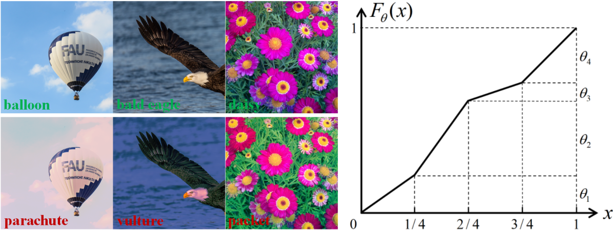
Building on these recent developments, we propose a new approach to generating unrestricted adversarial images using a color filter. The approach, called Adversarial Color Enhancement (ACE), introduces non-suspicious perturbations, with minimal impact on image quality, as shown in Figure 1 (left). Although previous work [Choi et al.(2017)Choi, Larson, Li, Li, Friedland, and Hanjalic] has pointed out that common enhancement practices (e.g., Instagram filters) can degrade the performance of the automatic geo-location estimation, until now, no research has focused on the optimization aspect of exploiting image filters to create adversarial images. Our approach makes use of recent advances in automatic image retouching based on differentiable approximation of commonly-used image filters  [Hu et al.(2018)Hu, He, Xu, Wang, and Lin, Deng et al.(2018)Deng, Loy, and Tang]. In sum, this paper makes the following contributions:

• We explore the vulnerability of the DNNs to commonly-used image filters, and specifically propose Adversarial Color Enhancement (ACE), an approach to generating unrestricted adversarial images by optimizing a differentiable color filter.

• Experimental results demonstrate ACE achieves a better trade-off between the adversarial strength and perceptual quality of the filtered images than other state-of-the-art methods, implying a stronger black-box adversary for real-world applications.

• We explore two potential ways to further improve ACE on image quality: 1) using widely-used enhancement practices (e.g., Instagram filters) as guidance to specified attractive image styles, and 2) leveraging regional semantic information.

2 Related Work

Differentiable Image Filters. The state of the art for automatic photo retouching mainly uses supervised learning to determine editing parameters via gradient descent, in order to achieve specific image appearances. Most approaches [Chen et al.(2017)Chen, Xu, and Koltun, Gharbi et al.(2017)Gharbi, Chen, Barron, Hasinoff, and Durand, Isola et al.(2017)Isola, Zhu, Zhou, and Efros, Yan et al.(2016)Yan, Zhang, Wang, Paris, and Yu, Zhu et al.(2017)Zhu, Park, Isola, and Efros] utilize DNNs for the parameterization of the editing process, but inevitably they suffer from high computational cost, fixed image resolution, and more importantly, a lack of interpretability. For this reason, some recent work [Hu et al.(2018)Hu, He, Xu, Wang, and Lin, Deng et al.(2018)Deng, Loy, and Tang] has proposed to rely on intuitively meaningful edits that are represented by conventional post-processing operations, i.e., image filters, to make the automatic process more understandable to users. Moreover, such methods have much fewer parameters to optimize, and can be applied resolution-independently.

Problem Formulation. A neural network can be denoted as a function $F(\boldsymbol{x})=\boldsymbol{y}$ that outputs $\boldsymbol{y}\in\mathbb{R}^{m}$ for an image $\boldsymbol{x}\in\mathbb{R}^{n}$. Here we focus on the widely-used DNN classifier with a softmax function, which expresses the output $\boldsymbol{y}$ as a probability distribution, i.e., $0\leq\boldsymbol{y}_{i}\leq 1$ and $\boldsymbol{y}_{1}+\cdot\cdot\cdot+\boldsymbol{y}_{m}=1$. The final predicted label $l$ for $\boldsymbol{x}$ is accordingly obtained by $l={\mathrm{argmax}}_{i}~{}\boldsymbol{y}_{i}$. An adversary aims to induce a misclassification of a DNN classifier $F(\boldsymbol{x})$ through modifying the original image $\boldsymbol{x}$ into $\boldsymbol{x}^{\prime}$ such that $F(\boldsymbol{x}^{\prime})\neq{y}$.

Restricted Adversary with Imperceptible Perturbations. As mentioned in Section 1, in order to make the modification unrecognizable, most existing work forces the adversarial image $\boldsymbol{x}^{\prime}$ to be visually close to its original image $\boldsymbol{x}$ with respect to specific distance measurements. The conventional solution is $L_{p}$ distance (typically $L_{\infty}$ [Carlini and Wagner(2017), Goodfellow et al.(2015)Goodfellow, Shlens, and Szegedy, Kurakin et al.(2017)Kurakin, Goodfellow, and Bengio, Madry et al.(2018)Madry, Makelov, Schmidt, Tsipras, and Vladu] and $L_{2}$ [Carlini and Wagner(2017), Moosavi-Dezfooli et al.(2016)Moosavi-Dezfooli, Fawzi, and Frossard, Rony et al.(2019)Rony, Hafemann, Oliveira, Ayed, Sabourin, and Granger, Szegedy et al.(2014)Szegedy, Zaremba, Sutskever, Bruna, Erhan, Goodfellow, and Fergus], but also $L_{1}$ [Chen et al.(2018a)Chen, Sharma, Zhang, Yi, and Hsieh] and $L_{0}$ [Papernot et al.(2016)Papernot, McDaniel, Jha, Fredrikson, Celik, and Swami, Su et al.(2019)Su, Vargas, and Sakurai]). The earliest work in this direction [Szegedy et al.(2014)Szegedy, Zaremba, Sutskever, Bruna, Erhan, Goodfellow, and Fergus] proposed to jointly optimize misclassification with cross-entropy loss and the $L_{2}$ distance by solving a box-constrained optimization with the L-BFGS method [Liu and Nocedal(1989)]. The C&W method [Carlini and Wagner(2017)] followed a similar idea, but replaced the cross-entropy loss with another specially designed loss function, namely, the differences between the pre-softmax logits. Moreover, a new variable was introduced to eliminate the box constraint. The method can be expressed as:

$$\begin{gathered}\underset{\boldsymbol{w}}{\mathrm{minimize}}~{}~{}{{\|\boldsymbol{x}^{\prime}-\boldsymbol{x}\|}_{2}^{2}}+\lambda f(\boldsymbol{x}^{\prime}),\\ \textrm{where}~{}~{}f(\boldsymbol{x}^{\prime})=\mathrm{max}(Z(\boldsymbol{x}^{\prime})_{l}-{\mathrm{max}}\{Z(\boldsymbol{x}^{\prime})_{i}:i\neq l\},-\kappa),\\ \textrm{and}~{}~{}\boldsymbol{x}^{\prime}=\frac{1}{2}(\tanh(\mathrm{arctanh}(\boldsymbol{x})+\boldsymbol{w})+1),\end{gathered}$$ (1)

where $f(\cdot)$ is the new loss function, $\boldsymbol{w}$ is the new variable, and $Z(x^{\prime})_{i}$ is the logit with respect to the $i$-th class given the intermediate modified image $\boldsymbol{x}^{\prime}$. The parameter $\kappa$ is applied to control the confidence level of the misclassification.

This joint optimization is straightforward but suffers from high computational cost due to the need for line search to optimize $\lambda$. For this reason, other methods [Goodfellow et al.(2015)Goodfellow, Shlens, and Szegedy, Dong et al.(2018)Dong, Liao, Pang, Su, Zhu, Hu, and Li, Kurakin et al.(2017)Kurakin, Goodfellow, and Bengio, Madry et al.(2018)Madry, Makelov, Schmidt, Tsipras, and Vladu, Rony et al.(2019)Rony, Hafemann, Oliveira, Ayed, Sabourin, and Granger] instead rely on Projected Gradient Descent (PGD) to restrict the perturbations with a small $L_{p}$ norm bound, $\epsilon$. Specifically, the fast gradient sign method (FGSM) [Goodfellow et al.(2015)Goodfellow, Shlens, and Szegedy] was designed to succeed within only one step and was extended by [Dong et al.(2018)Dong, Liao, Pang, Su, Zhu, Hu, and Li, Kurakin et al.(2017)Kurakin, Goodfellow, and Bengio, Madry et al.(2018)Madry, Makelov, Schmidt, Tsipras, and Vladu, Rony et al.(2019)Rony, Hafemann, Oliveira, Ayed, Sabourin, and Granger] to exploit finer gradient information with multiple iterations. The iterative approach can be formulated as:

$${\boldsymbol{x}_{0}^{\prime}}=\boldsymbol{x},~{}~{}{\boldsymbol{x}_{k}^{\prime}}={\boldsymbol{x}_{k-1}^{\prime}}+\alpha\cdot\ \mathrm{sign}({\nabla_{{\boldsymbol{x}}}J(\boldsymbol{x}_{k-1}^{\prime},l)}),$$ (2)

where $\alpha$ denotes the step size in each iteration. The generated adversarial perturbations will be clipped to satisfy the $L_{\infty}$ bound. A generalization of this formulation to the $L_{2}$ norm can be achieved by replacing the $\mathrm{sign}(\cdot)$ with a normalization operation [Moosavi-Dezfooli et al.(2016)Moosavi-Dezfooli, Fawzi, and Frossard, Rony et al.(2019)Rony, Hafemann, Oliveira, Ayed, Sabourin, and Granger]. $L_{0}$ and $L_{1}$-bounded adversarial images were also studied [Chen et al.(2018a)Chen, Sharma, Zhang, Yi, and Hsieh, Papernot et al.(2016)Papernot, McDaniel, Jha, Fredrikson, Celik, and Swami, Su et al.(2019)Su, Vargas, and Sakurai], but not widely adopted since the resulting sparse perturbations are not stable in practice.

Recently, there have also been several attempts to address the limitations of naive $L_{p}$ by using more perception-aligned solutions for measuring similarity. A straightforward way is by incorporating existing metrics, such as Structural SIMilarity (SSIM) [Rozsa et al.(2016)Rozsa, Rudd, and Boult], Wasserstein distance [Wong et al.(2019)Wong, Schmidt, and Kolter], and the perceptual color metric CIEDE2000 [Zhao et al.(2020)Zhao, Liu, and Larson]. Other methods [Croce and Hein(2019), Luo et al.(2018)Luo, Liu, Wei, and Xu, Zhang et al.(2020)Zhang, Avrithis, Furon, and Amsaleg] adapted the $L_{p}$ measurements to the textural properties of the image, i.e., hiding perturbations in image regions with high visual variation. Local pixel displacement was also explored [Xiao et al.(2018)Xiao, Zhu, Li, He, Liu, and Song, Alaifari et al.(2019)Alaifari, Alberti, and Gauksson]. In general, these solutions yield a better trade-off between adversarial strength and imperceptibility than conventional $L_{p}$ methods.

Unrestricted Adversaries towards Realistic Images. Due to the assumption of imperceptible perturbations, now considered unrealistic, as mentioned in Section 1, recent work has started to pursue non-suspicious adversarial images with large perturbations, which make more sense in practical use scenarios. Common approaches to creating such unrestricted adversarial images can be divided into three categories: geometric transformation, semantic manipulation, and color modification. The geometric transformation method penalizes image differences with respect to small rotations and translations of the image [Engstrom et al.(2019)Engstrom, Tran, Tsipras, Schmidt, and Madry]. Semantic manipulation has been so far mainly studied in the domain of face recognition, where the perturbation is optimized with respect to specific semantic attribute(s), such as colors of skin and extent of makeup [Joshi et al.(2019)Joshi, Mukherjee, Sarkar, and Hegde, Qiu et al.(2020)Qiu, Xiao, Yang, Yan, Lee, and Li, Sharif et al.(2019)Sharif, Bhagavatula, Bauer, and Reiter].

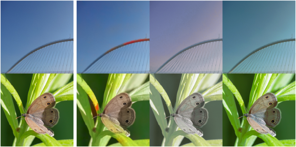
Existing colorization-based work has explored uniform color transformation [Hosseini and Poovendran(2018), Laidlaw and Feizi(2019), Shamsabadi et al.(2020)Shamsabadi, Sanchez-Matilla, and Cavallaro] and automatic colorization [Bhattad et al.(2020)Bhattad, Chong, Liang, Li, and Forsyth]. Specifically, the early method [Hosseini and Poovendran(2018)] randomly adjusts the hue values of each image pixel to search for possible adversarial images. The ColorFool method [Shamsabadi et al.(2020)Shamsabadi, Sanchez-Matilla, and Cavallaro] improves on [Hosseini and Poovendran(2018)] by imposing semantic-aware norm constraints for better image quality, but still relies on costly random search. The ReColorAdv method [Laidlaw and Feizi(2019)] optimizes color transformation over a discretely parameterized color space with post-interpolation and regularization on local uniformity, and impose $L_{\infty}$ bounds on the perturbations. The cAdv method [Bhattad et al.(2020)Bhattad, Chong, Liang, Li, and Forsyth] takes a different route, optimizing a pre-trained automatic colorization model to re-colorize the gray-scale version of the original image. It increases the computational overhead due to the huge number of parameters in the deep colorization model, and also has been shown to cause abnormal color stains (see examples in  [Bhattad et al.(2020)Bhattad, Chong, Liang, Li, and Forsyth] and our Figure 3).

Our ACE falls into the colorization category but is markedly different from existing approaches. Specifically, ACE creates adversarial images by optimizing with gradient information, and, in this way, is fundamentally different from the random search-based approaches in [Hosseini and Poovendran(2018), Shamsabadi et al.(2020)Shamsabadi, Sanchez-Matilla, and Cavallaro]. In Section 4, we also show that our gradient-based ACE outperforms its alternative with random search. Our color filter is simpler and more transparent than the deep colorization model in [Bhattad et al.(2020)Bhattad, Chong, Liang, Li, and Forsyth]. Compared with [Laidlaw and Feizi(2019)], our ACE enjoys a more elegant and continuous formulation. Experimental results in Section 4 demonstrate that our ACE outperforms these approaches in both adversarial strength and image quality.

3 Adversarial Color Enhancement (ACE)

This section describes our proposed Adversarial Color Enhancement (ACE), which generates visually realistic adversarial filtered images based on a commonly-used color filter. Specifically, we adopt the differentiable approximation in  [Hu et al.(2018)Hu, He, Xu, Wang, and Lin] to parameterize the color filter by a monotonic piecewise-linear mapping function with totally $K$ pieces:

$$\begin{gathered}F_{\boldsymbol{\theta}}(x_{k})=\sum\limits_{i=1}^{k-1}{\theta_{i}}+(K\cdot x_{k}-(k-1))\cdot\theta_{k},\\ \textrm{s.t.}~{}0\leq\theta_{i}\leq 1~{}\mathrm{and}~{}\sum_{i}\theta_{i}=1,\end{gathered}$$ (3)

where $x_{k}$ denotes any image pixel whose value falls into the $k$-th piece of the mapping function, and $F_{\boldsymbol{\theta}}(x_{k})$ is its corresponding output after filtering. An example of this function with four pieces ($K=4$) is illustrated in Figure 1 (right).

Note that we are not optimizing in the pixel space but in the latent space of filter parameters, and the three RGB channels are operated on in parallel. The parameters $\boldsymbol{\theta}$ ($K$ in total) can be optimized via gradient descent to achieve a specific objective. Obviously, an image will remain unchanged ($F_{\boldsymbol{\theta}}(x)=x$) when all the parameters are equal to $1/K$. As a result, we propose to control over the adjustment by imposing constraints on the distance between each parameter and its initial value $1/K$. The misclassification objective and the proposed constraints on the parameters will be jointly optimized with a balance factor $\lambda$, expressed as:

$$\underset{\boldsymbol{\theta}}{\mathrm{minimize}}~{}f(F_{\boldsymbol{\theta}}(\boldsymbol{x}))+\lambda\cdot\sum_{i}({\theta_{i}}-1/K)^{2},$$ (4)

where $f(\cdot)$ is the C&W loss on logit differences in Equation 1.

	$\rightarrow$Alex	$\rightarrow$R50	$\rightarrow$V19	$\rightarrow$D121	$\rightarrow$Inc3
Alex	99.9	6.26	7.10	6.85	2.08
R50	48.50	98.3	15.83	13.21	5.96
V19	39.52	11.29	98.5	10.65	10.30
D121	46.50	18.51	15.16	98.4	5.61
Inc3	41.12	16.42	14.87	12.35	93.2

	$\rightarrow$Alex	$\rightarrow$R18	$\rightarrow$R50
Alex	100.0	16.40	12.30
R18	48.52	99.2	22.43
R50	48.98	30.47	99.0

Table 1: White-box success rates (diagonal) and black-box transferability of our ACE in ImageNet classification (left) and private scene recognition (right). Considered models: AlexNet (Alex), ResNet18 (R18), ResNet50 (R50), VGG19 (V19), DenseNet121 (D121), and Inception-V3 (Inc3). The success rates are measured with respect to the models in the columns when applying ACE on the models in the rows.

4 Experiments

We evaluate our ACE in two different tasks: object classification and scene recognition, and consider the following two datasets. ImageNet-Compatible dataset consists of 6000 images associated with ImageNet class labels, and has been used in the NIPS 2017 Competition on Adversarial Attacks and Defenses [Kurakin et al.(2018)Kurakin, Goodfellow, Bengio, Dong, Liao, Liang, Pang, Zhu, Hu, Xie, et al.]. Here we use its development set containing 1000 images. Private Scene dataset was introduced by the MediaEval Pixel Privacy task [Larson et al.(2018)Larson, Liu, Brugman, and Zhao], which aims to develop image modification techniques that help to protect users against automatic inference of privacy-sensitive scene information. It contains 600 images with 60 privacy-sensitive scene categories, selected from the Places365 dataset [Zhou et al.(2017)Zhou, Lapedriza, Khosla, Oliva, and Torralba]. For the ImageNet task, we consider five distinct classifiers that are pre-trained on ImageNet: AlexNet [Krizhevsky et al.(2012)Krizhevsky, Sutskever, and Hinton], ResNet50 [He et al.(2016)He, Zhang, Ren, and Sun], VGG19 [Simonyan and Zisserman(2015)], DenseNet121 [Huang et al.(2017)Huang, Liu, Van Der Maaten, and Weinberger], and Inception-V3 [Szegedy et al.(2016)Szegedy, Vanhoucke, Ioffe, Shlens, and Wojna]. For the scene task, we consider AlexNet, ResNet18, and ResNet50 pre-trained on the Places365 dataset.

Our experiments are carried out on a single NVIDIA Tesla P100 GPU with 12 GB of memory. ACE is optimized using Adam [Kingma and Ba(2014)] with a learning rate of 0.01, under a maximum budget of 500 iterations. We execute the optimization in 40 batches of 25 image samples, and the run-time on ImageNet task is about 2 seconds per image. Early stopping is triggered when the optimization is no longer making progress as implemented in [Carlini and Wagner(2017), Rony et al.(2019)Rony, Hafemann, Oliveira, Ayed, Sabourin, and Granger]. If not mentioned specifically, ACE is implemented with the optimal settings, $K=64$ and $\lambda=5$. Table 1 shows that our ACE can achieve high white-box success rates and have good cross-model transferability. It can also be observed that models with more sophisticated architecture are generally harder to fool in the white-box case, and transferring from a sophisticated architecture to a simple one is easier than the other way around. Note that the transferability is calculated on images for which the prediction of both the models involved is the same.

	$L_{p}$ Norm			Success Rate
	$L_{0}$ (%)	$L_{2}$	$L_{\infty}$	Inc3	$\rightarrow$Alex	$\rightarrow$R50	$\rightarrow$V19	$\rightarrow$D121
FGSM [Goodfellow et al.(2015)Goodfellow, Shlens, and Szegedy]	49.34	4.05	2.00	78.10	7.84	5.40	5.74	5.50
BIM [Kurakin et al.(2017)Kurakin, Goodfellow, and Bengio]	39.23	3.09	2.00	99.1	8.16	4.95	6.44	4.71
C&W [Carlini and Wagner(2017)]	29.06	3.00	15.66	99.6	8.16	4.72	6.79	4.38
ReColorAdv [Laidlaw and Feizi(2019)]	70.81	18.87	64.00	79.3	9.76	4.50	3.40	2.58
ReColorAdv+ [Laidlaw and Feizi(2019)]	82.50	47.53	97.21	89.2	31.20	15.64	13.58	10.77
cAdv [Bhattad et al.(2020)Bhattad, Chong, Liang, Li, and Forsyth]	41.42	20.54	116.15	91.8	30.08	11.25	11.01	13.47
Our ACE	42.99	40.61	45.98	93.2	41.12	16.42	14.87	12.35

Table 2: White-box success rates and black-box transferability of our ACE compared with other baselines. $L_{0}$ is the proportion of the perturbed pixels and $L_{\infty}$ is shown in [0,255]. Here the Inception-V3 is used as the target white-box model.

4.1 Comparisons on Adversarial Strength and Image Quality

We further compare ACE with the following gradient-based baseline methods in terms of adversarial strength and image quality, in the ImageNet task:

FGSM [Goodfellow et al.(2015)Goodfellow, Shlens, and Szegedy] with a $L_{\infty}$ norm bound $\epsilon=2/255$ for ensuring imperceptibility.

BIM [Kurakin et al.(2017)Kurakin, Goodfellow, and Bengio] with a $L_{\infty}$ norm bound $\epsilon=2/255$, and 10 iterations of gradient descent.

C&W [Carlini and Wagner(2017)] optimized on $L_{2}$ with fewer iterations and higher confidence level (iters=$3\times 100$ and $\kappa=40$) than usual to yield larger perturbations for stronger adversarial effects.

ReColorAdv [Laidlaw and Feizi(2019)] (Unrestricted) with $\epsilon=16/255$ and lr=0.001 as in [Laidlaw and Feizi(2019)], and another version allowing larger perturbations ($\epsilon=51/255$ and lr=0.005), denoted as ReColorAdv⁺.

cAdv [Bhattad et al.(2020)Bhattad, Chong, Liang, Li, and Forsyth] (Unrestricted) with the settings leading to optimal color realism ($k=8$). Note that cAdv can only produce adversarial images sized $224\times 224$ due to the fixed output resolution of its pre-trained deep colorization model.

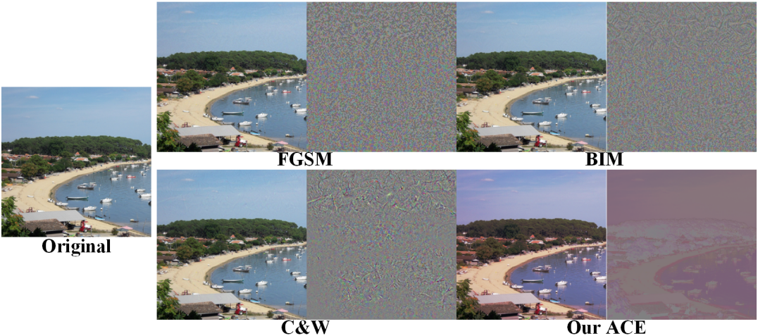
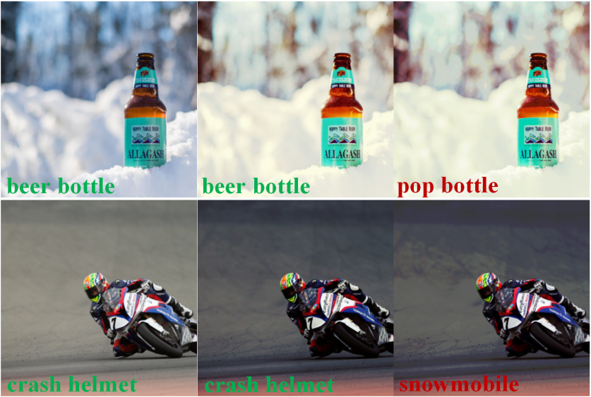
We adopt Inception-V3 as the white-box model because it is the official model used in the NIPS 2017 Competition. As shown in Table 2, ACE can consistently achieve better transferability than conventional $L_{p}$ methods, while not introducing visually suspicious noisy patterns (see Figure 2). Iterative $L_{p}$ methods (BIM and C&W) could achieve the strongest white-box adversarial effects by fully leveraging the gradient information, but these effects are less generalizable to other unseen models, i.e., worse transferability. Among the unrestricted methods, our ACE achieves the highest white-box success rates and overall best transferability, while yielding smooth adjustment without abnormal colorization artifacts (see Figure 3). Such smoothness is also reflected in $L_{\infty}$ norms that are lower than other unrestricted methods, meaning that ACE tends to avoid excessive local color changes.

Figure 2: Adversarial images and perturbations by our ACE and $L_{p}$ methods FGSM [Goodfellow et al.(2015)Goodfellow, Shlens, and Szegedy], BIM [Kurakin et al.(2017)Kurakin, Goodfellow, and Bengio] and C&W [Carlini and Wagner(2017)]. ACE yields more natural appearances without abnormal patterns.

Figure 3: Examples from three different unrestricted methods. From left to right: original image, adversarial images generated by cAdv [Bhattad et al.(2020)Bhattad, Chong, Liang, Li, and Forsyth], ReColorAdv⁺ [Laidlaw and Feizi(2019)], and our ACE. ACE yields more acceptable images with smooth appearances and fewer artifacts.

4.2 Ablation Study

Hyperparameters. Figure 4 (left) shows the success rates of ACE with a different number of pieces $K$ under different factor $\lambda$ values used for balancing the two loss terms in the joint optimization. We can observe that increasing $K$ slightly improves the performance by expanding the action space of the adversary. Moreover, increasing $K$ allows more fine-grained color adjustment in the images that have rich colors. It should also be noted that using more pieces means more computational cost during the optimization.

Figure 4: Left: White-box success rates of ACE when varying the number of pieces $K$ with four different $\lambda$ values. Right: Adversarial images with varied $\lambda$. For each example, from left to right: original image, adversarial images with $\lambda=$10, 5 and 0. Too large a $\lambda$ makes ACE not reach its full potential, while setting $\lambda=0$ may cause unrealistic colorization.

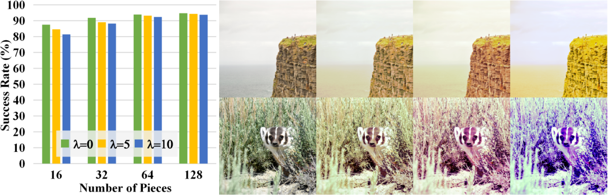
On the other hand, relaxing the constraints by decreasing $\lambda$ gives the adversary larger action space, leading to higher success rates. However, completely removing the constraints ($\lambda=0$) will lead to unrealistic image appearances, as can be observed in Figure 4 (right). Specifically, in this paper, we use $K=64$ and $\lambda=5$ as optimal settings for a good trade-off.

Gradient Descent vs. Random Search. We compare our gradient-based ACE with a random search-based implementation using the same color filter. In this case, the parameters will be updated with gradient information in our ACE, while being uniformly sampled from the valid range [0,1] for random search.

Figure 5: White-box success rates for our ACE (left) and random search (right) as a function of maximum allowed iterations. Note that the scales on the two x-axes are not the same.

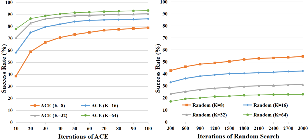
Figure 5 shows their white-box success rates as a function of iterations. For random search, we repeat several times and got almost the same results. We can observe that our ACE consistently outperforms random search, even with far fewer iterations. Moreover, ACE gradually improves as the number of parameters $K$ increases, indicating that it can benefit from the expanded action space for more fine-grained color adjustment. In contrast, random search becomes increasingly worse since the potentially successful adversarial samples can no longer be feasibly found in the exponentially expanded parameter space. For comparison we mention that, the grid search-based ColorFool [Shamsabadi et al.(2020)Shamsabadi, Sanchez-Matilla, and Cavallaro] has a success rate of 64.6% (65.4%) with 1000 (1500) iterations when testing on our dataset with the Inception-V3 as the white-box model.

Figure 6: Adversarial filtered images by ACE with guidance of specific image filters. Two Instagram filters are considered: Hefe (top) and Gotham (bottom). For each, from left to right: original image, Instagram filtered image and adversarial filtered image by ACE.

Figure 7: Adapting ACE on different semantics. Original image (left), successful adversary with stronger constraints for cat but weaker for blanket (middle), or vice versa (right). The middle case yields more realistic results since blanket naturally occurs with various colors.

5 ACE Extensions

Adaption on Image Styles. Previous work [Choi et al.(2017)Choi, Larson, Li, Li, Friedland, and Hanjalic] has pointed out that popular image enhancement practices can potentially degrade automatic inference. Despite our ACE in Equation 4 achieving visually acceptable results, it is not directly optimized towards enhancing image quality. Therefore, we explore the possibility to guide ACE towards achieving quality enhancement in addition to the adversarial effects. Specifically, we propose to optimize the adversarial image towards specific attractive styles that were obtained by using Instagram filters. Accordingly, the optimization objective is adjusted to:

$$\underset{\boldsymbol{\theta}}{\mathrm{minimize}}~{}f(F_{\boldsymbol{\theta}}(\boldsymbol{x}))+\lambda\cdot{\|F_{\boldsymbol{\theta}}(\boldsymbol{x})-\boldsymbol{x}_{t}\|}_{2}^{2},$$ (5)

where $\boldsymbol{x}_{t}$ denotes the target Instagram filtered image, and the final adversarial filtered image $F_{\boldsymbol{\theta}}$ is therefore guided to have similar appearances with $\boldsymbol{x}_{t}$ by minimizing their distance. As shown in Figure 6, this adaptation of ACE can successfully enhance the image by mimicking the effects of Instagram filters.

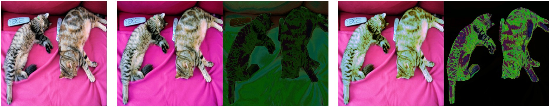
Adaptation on Semantics. ACE treats all the image pixels that have the same values in the same way. Inspired by previous work [Bhattad et al.(2020)Bhattad, Chong, Liang, Li, and Forsyth, Shamsabadi et al.(2020)Shamsabadi, Sanchez-Matilla, and Cavallaro], we show that semantically adapting ACE could better maintain image quality by hiding large perturbations in the semantic regions that remain realistic with various colors. Specifically, Equation 4 is adapted to:

$$\underset{\boldsymbol{\theta}}{\mathrm{min}}~{}\sum_{n}[J(F_{\boldsymbol{\theta}_{n}}(\boldsymbol{x}\cdot M_{n}))+\lambda\sum_{i}w_{n}\cdot({\theta_{n_{i}}}-1/K)^{2}],~{}\textrm{s.t.}~{}\sum_{n}w_{n}=1,$$ (6)

where $w_{n}$ is the weight for the $n$-th filter, $F_{\boldsymbol{\theta}}^{n}(\cdot)$, which is optimized independently for a specific semantic region given its mask $M_{n}$ obtained by a semantic segmentation method [Kirillov et al.(2019)Kirillov, Girshick, He, and Dollár]. As shown in Figure 7, this adaption avoids raising the sense of unrealistic colorization, leading to improved image quality.

6 Conclusion

We have proposed Adversarial Color Enhancement (ACE), an approach to generating unrestricted adversarial images by optimizing a color filter via gradient descent. ACE has been shown to produce realistic filtered images with good transferability, which results in strong real-world black-box adversaries. We also present two potential ways to improve ACE in terms of image quality by guiding it with specific attractive image styles or adapting it to regional semantics.

In the current ACE, the single hyperparameter of the filter ($K$ in Equation 3) is per-fixed for all images without considering their individual properties. Since natural images would differ in the range and complexity of their contained colors, adaptive strategies would be worth exploring in order to yield more suitable modifications. For example, images with most pixels concentrated in a certain color range should have larger action space in that range than those with more uniform color distribution. It would also be interesting to carry out user study on the visual quality of the images generated by ACE. On the other side, developing defenses against the proposed adversarial color filtering is necessary to make current neural networks more robust, based on either adversarial training or algorithms for identifying adversarial modifications by ACE.

References

- [Alaifari et al.(2019)Alaifari, Alberti, and Gauksson] Rima Alaifari, Giovanni S Alberti, and Tandri Gauksson. ADef: an iterative algorithm to construct adversarial deformations. In ICLR, 2019.
- [Arnab et al.(2018)Arnab, Miksik, and Torr] Anurag Arnab, Ondrej Miksik, and Philip HS Torr. On the robustness of semantic segmentation models to adversarial attacks. In CVPR, 2018.
- [Bhattad et al.(2020)Bhattad, Chong, Liang, Li, and Forsyth] Anand Bhattad, Min Jin Chong, Kaizhao Liang, Bo Li, and David A Forsyth. Unrestricted adversarial examples via semantic manipulation. In ICLR, 2020.
- [Brown et al.(2018)Brown, Carlini, Zhang, Olsson, Christiano, and Goodfellow] Tom B Brown, Nicholas Carlini, Chiyuan Zhang, Catherine Olsson, Paul Christiano, and Ian Goodfellow. Unrestricted adversarial examples. In arXiv preprint, 2018.
- [Carlini and Wagner(2017)] Nicholas Carlini and David Wagner. Towards evaluating the robustness of neural networks. In IEEE S&P, 2017.
- [Chen et al.(2018a)Chen, Sharma, Zhang, Yi, and Hsieh] Pin-Yu Chen, Yash Sharma, Huan Zhang, Jinfeng Yi, and Cho-Jui Hsieh. EAD: elastic-net attacks to deep neural networks via adversarial examples. In AAAI, 2018a.
- [Chen et al.(2017)Chen, Xu, and Koltun] Qifeng Chen, Jia Xu, and Vladlen Koltun. Fast image processing with fully-convolutional networks. In ICCV, 2017.
- [Chen et al.(2018b)Chen, Cornelius, Martin, and Chau] Shang-Tse Chen, Cory Cornelius, Jason Martin, and Duen Horng Polo Chau. Shapeshifter: Robust physical adversarial attack on faster r-cnn object detector. In ECML PKDD, 2018b.
- [Choi et al.(2017)Choi, Larson, Li, Li, Friedland, and Hanjalic] Jaeyoung Choi, Martha Larson, Xinchao Li, Kevin Li, Gerald Friedland, and Alan Hanjalic. The geo-privacy bonus of popular photo enhancements. In ICMR, 2017.
- [Croce and Hein(2019)] Francesco Croce and Matthias Hein. Sparse and imperceivable adversarial attacks. In ICCV, 2019.
- [Deng et al.(2018)Deng, Loy, and Tang] Yubin Deng, Chen Change Loy, and Xiaoou Tang. Aesthetic-driven image enhancement by adversarial learning. In ACM MM, 2018.
- [Dong et al.(2018)Dong, Liao, Pang, Su, Zhu, Hu, and Li] Yinpeng Dong, Fangzhou Liao, Tianyu Pang, Hang Su, Jun Zhu, Xiaolin Hu, and Jianguo Li. Boosting adversarial attacks with momentum. In CVPR, 2018.
- [Engstrom et al.(2019)Engstrom, Tran, Tsipras, Schmidt, and Madry] Logan Engstrom, Brandon Tran, Dimitris Tsipras, Ludwig Schmidt, and Aleksander Madry. Exploring the landscape of spatial robustness. In ICML, 2019.
- [Gharbi et al.(2017)Gharbi, Chen, Barron, Hasinoff, and Durand] Michaël Gharbi, Jiawen Chen, Jonathan T Barron, Samuel W Hasinoff, and Frédo Durand. Deep bilateral learning for real-time image enhancement. ACM Transactions on Graphics, 36(4):1–12, 2017.
- [Gilmer et al.(2018)Gilmer, Adams, Goodfellow, Andersen, and Dahl] Justin Gilmer, Ryan P Adams, Ian Goodfellow, David Andersen, and George E Dahl. Motivating the rules of the game for adversarial example research. In arXiv preprint, 2018.
- [Goodfellow et al.(2015)Goodfellow, Shlens, and Szegedy] Ian Goodfellow, Jonathon Shlens, and Christian Szegedy. Explaining and harnessing adversarial examples. In ICLR, 2015.
- [He et al.(2016)He, Zhang, Ren, and Sun] Kaiming He, Xiangyu Zhang, Shaoqing Ren, and Jian Sun. Deep residual learning for image recognition. In CVPR, 2016.
- [Hosseini and Poovendran(2018)] Hossein Hosseini and Radha Poovendran. Semantic adversarial examples. In CVPR Workshops, 2018.
- [Hu et al.(2018)Hu, He, Xu, Wang, and Lin] Yuanming Hu, Hao He, Chenxi Xu, Baoyuan Wang, and Stephen Lin. Exposure: A white-box photo post-processing framework. ACM Transactions on Graphics, 37(2):26, 2018.
- [Huang et al.(2017)Huang, Liu, Van Der Maaten, and Weinberger] Gao Huang, Zhuang Liu, Laurens Van Der Maaten, and Kilian Q Weinberger. Densely connected convolutional networks. In CVPR, 2017.
- [Isola et al.(2017)Isola, Zhu, Zhou, and Efros] Phillip Isola, Jun-Yan Zhu, Tinghui Zhou, and Alexei A Efros. Image-to-image translation with conditional adversarial networks. In CVPR, 2017.
- [Joshi et al.(2019)Joshi, Mukherjee, Sarkar, and Hegde] Ameya Joshi, Amitangshu Mukherjee, Soumik Sarkar, and Chinmay Hegde. Semantic adversarial attacks: Parametric transformations that fool deep classifiers. In ICCV, 2019.
- [Kingma and Ba(2014)] Diederik P. Kingma and Jimmy Ba. Adam: A method for stochastic optimization. In ICLR, 2014.
- [Kirillov et al.(2019)Kirillov, Girshick, He, and Dollár] Alexander Kirillov, Ross Girshick, Kaiming He, and Piotr Dollár. Panoptic feature pyramid networks. In CVPR, 2019.
- [Krizhevsky et al.(2012)Krizhevsky, Sutskever, and Hinton] Alex Krizhevsky, Ilya Sutskever, and Geoffrey E Hinton. Imagenet classification with deep convolutional neural networks. In NeurIPS, 2012.
- [Kurakin et al.(2017)Kurakin, Goodfellow, and Bengio] Alexey Kurakin, Ian Goodfellow, and Samy Bengio. Adversarial examples in the physical world. In ICLR, 2017.
- [Kurakin et al.(2018)Kurakin, Goodfellow, Bengio, Dong, Liao, Liang, Pang, Zhu, Hu, Xie, et al.] Alexey Kurakin, Ian Goodfellow, Samy Bengio, Yinpeng Dong, Fangzhou Liao, Ming Liang, Tianyu Pang, Jun Zhu, Xiaolin Hu, Cihang Xie, et al. Adversarial attacks and defences competition. In The NIPS’17 Competition: Building Intelligent Systems, 2018.
- [Laidlaw and Feizi(2019)] Cassidy Laidlaw and Soheil Feizi. Functional adversarial attacks. In NeurIPS, 2019.
- [Larson et al.(2018)Larson, Liu, Brugman, and Zhao] Martha Larson, Zhuoran Liu, Simon Brugman, and Zhengyu Zhao. Pixel privacy: Increasing image appeal while blocking automatic inference of sensitive scene information. In MediaEval Multimedia Benchmark Workshop, 2018.
- [Liu and Nocedal(1989)] Dong C Liu and Jorge Nocedal. On the limited memory BFGS method for large scale optimization. Mathematical Programming, 45(1-3):503–528, 1989.
- [Liu et al.(2019)Liu, Zhao, and Larson] Zhuoran Liu, Zhengyu Zhao, and Martha Larson. Who’s afraid of adversarial queries? The impact of image modifications on content-based image retrieval. In ICMR, 2019.
- [Luo et al.(2018)Luo, Liu, Wei, and Xu] Bo Luo, Yannan Liu, Lingxiao Wei, and Qiang Xu. Towards imperceptible and robust adversarial example attacks against neural networks. In AAAI, 2018.
- [Madry et al.(2018)Madry, Makelov, Schmidt, Tsipras, and Vladu] Aleksander Madry, Aleksandar Makelov, Ludwig Schmidt, Dimitris Tsipras, and Adrian Vladu. Towards deep learning models resistant to adversarial attacks. In ICLR, 2018.
- [Moosavi-Dezfooli et al.(2016)Moosavi-Dezfooli, Fawzi, and Frossard] Seyed-Mohsen Moosavi-Dezfooli, Alhussein Fawzi, and Pascal Frossard. DeepFool: a simple and accurate method to fool deep neural networks. In CVPR, 2016.
- [Papernot et al.(2016)Papernot, McDaniel, Jha, Fredrikson, Celik, and Swami] Nicolas Papernot, Patrick McDaniel, Somesh Jha, Matt Fredrikson, Z Berkay Celik, and Ananthram Swami. The limitations of deep learning in adversarial settings. In IEEE EuroS&P, 2016.
- [Qiu et al.(2020)Qiu, Xiao, Yang, Yan, Lee, and Li] Haonan Qiu, Chaowei Xiao, Lei Yang, Xinchen Yan, Honglak Lee, and Bo Li. Semanticadv: Generating adversarial examples via attribute-conditional image editing. In ECCV, 2020.
- [Rony et al.(2019)Rony, Hafemann, Oliveira, Ayed, Sabourin, and Granger] Jérôme Rony, Luiz G. Hafemann, Luiz S. Oliveira, Ismail Ben Ayed, Robert Sabourin, and Eric Granger. Decoupling direction and norm for efficient gradient-based adversarial attacks and defenses. In CVPR, 2019.
- [Rozsa et al.(2016)Rozsa, Rudd, and Boult] Andras Rozsa, Ethan M Rudd, and Terrance E Boult. Adversarial diversity and hard positive generation. In CVPR Workshops, 2016.
- [Shamsabadi et al.(2020)Shamsabadi, Sanchez-Matilla, and Cavallaro] Ali Shahin Shamsabadi, Ricardo Sanchez-Matilla, and Andrea Cavallaro. ColorFool: Semantic adversarial colorization. In CVPR, 2020.
- [Sharif et al.(2018)Sharif, Bauer, and Reiter] Mahmood Sharif, Lujo Bauer, and Michael K. Reiter. On the suitability of -norms for creating and preventing adversarial examples. In CVPR Workshops, 2018.
- [Sharif et al.(2019)Sharif, Bhagavatula, Bauer, and Reiter] Mahmood Sharif, Sruti Bhagavatula, Lujo Bauer, and Michael K. Reiter. A general framework for adversarial examples with objectives. ACM Transactions on Privacy and Security, 2019.
- [Simonyan and Zisserman(2015)] Karen Simonyan and Andrew Zisserman. Very deep convolutional networks for large-scale image recognition. In ICLR, 2015.
- [Su et al.(2019)Su, Vargas, and Sakurai] Jiawei Su, Danilo Vasconcellos Vargas, and Kouichi Sakurai. One pixel attack for fooling deep neural networks. IEEE Transactions on Evolutionary Computation, 23(5):828–841, 2019.
- [Szegedy et al.(2014)Szegedy, Zaremba, Sutskever, Bruna, Erhan, Goodfellow, and Fergus] Christian Szegedy, Wojciech Zaremba, Ilya Sutskever, Joan Bruna, Dumitru Erhan, Ian Goodfellow, and Rob Fergus. Intriguing properties of neural networks. In ICLR, 2014.
- [Szegedy et al.(2016)Szegedy, Vanhoucke, Ioffe, Shlens, and Wojna] Christian Szegedy, Vincent Vanhoucke, Sergey Ioffe, Jon Shlens, and Zbigniew Wojna. Rethinking the Inception architecture for computer vision. In CVPR, 2016.
- [Tolias et al.(2019)Tolias, Radenovic, and Chum] Giorgos Tolias, Filip Radenovic, and Ondrej Chum. Targeted mismatch adversarial attack: Query with a flower to retrieve the tower. In ICCV, 2019.
- [Wang et al.(2004)Wang, Bovik, Sheikh, and Simoncelli] Zhou Wang, Alan C. Bovik, Hamid R. Sheikh, and Eero P. Simoncelli. Image quality assessment: from error visibility to structural similarity. IEEE Transactions on Image Processing, 13(4):600–612, 2004.
- [Wong et al.(2019)Wong, Schmidt, and Kolter] Eric Wong, Frank Schmidt, and Zico Kolter. Wasserstein adversarial examples via projected sinkhorn iterations. In ICML, 2019.
- [Xiao et al.(2018)Xiao, Zhu, Li, He, Liu, and Song] Chaowei Xiao, Jun-Yan Zhu, Bo Li, Warren He, Mingyan Liu, and Dawn Song. Spatially transformed adversarial examples. In ICLR, 2018.
- [Xie et al.(2017)Xie, Wang, Zhang, Zhou, Xie, and Yuille] Cihang Xie, Jianyu Wang, Zhishuai Zhang, Yuyin Zhou, Lingxi Xie, and Alan Yuille. Adversarial examples for semantic segmentation and object detection. In ICCV, 2017.
- [Yan et al.(2016)Yan, Zhang, Wang, Paris, and Yu] Zhicheng Yan, Hao Zhang, Baoyuan Wang, Sylvain Paris, and Yizhou Yu. Automatic photo adjustment using deep neural networks. ACM Transactions on Graphics, 35(2):1–15, 2016.
- [Zhang et al.(2020)Zhang, Avrithis, Furon, and Amsaleg] Hanwei Zhang, Yannis Avrithis, Teddy Furon, and Laurent Amsaleg. Smooth adversarial examples. EURASIP Journal on Information Security, 2020.
- [Zhao et al.(2019)Zhao, Zhu, Liang, Shen, Zhang, and Chen] Yue Zhao, Hong Zhu, Ruigang Liang, Qintao Shen, Shengzhi Zhang, and Kai Chen. Seeing isn’t believing: Towards more robust adversarial attack against real world object detectors. In ACM CCS, 2019.
- [Zhao et al.(2020)Zhao, Liu, and Larson] Zhengyu Zhao, Zhuoran Liu, and Martha Larson. Towards large yet imperceptible adversarial image perturbations with perceptual color distance. In CVPR, 2020.
- [Zhou et al.(2017)Zhou, Lapedriza, Khosla, Oliva, and Torralba] Bolei Zhou, Agata Lapedriza, Aditya Khosla, Aude Oliva, and Antonio Torralba. Places: A 10 million image database for scene recognition. IEEE Transactions on Pattern Analysis and Machine Intelligence, 40(6):1452–1464, 2017.
- [Zhu et al.(2017)Zhu, Park, Isola, and Efros] Jun-Yan Zhu, Taesung Park, Phillip Isola, and Alexei A Efros. Unpaired image-to-image translation using cycle-consistent adversarial networks. In ICCV, 2017.