Suppression of the Higgs Dimuon Decay
Abstract
It is often stated that elimination of tree-level flavor-changing neutral currents in multi-Higgs models requires that all fermions of a given charge to couple to the same Higgs boson. A counterexample was provided by Abe, Sato and Yagyu (ASY) in a muon-specific two-Higgs doublet model. In this model, all fermions except the muon couple to one Higgs and the muon couples to the other. We study the phenomenology of the model and show that there is a wide range of parameter-space in which the branching ratios of the 125 GeV Higgs are very close to their Standard Model values, with the exception of the branching ratio into muons, which can be substantially suppressed – this is an interesting possibility, since the current value of this branching ratio is times the Standard Model value. We also study the charged Higgs boson and show that, if it is lighter than GeV, it could have a large branching ratio into - even substantially larger than the usual decay into . The decays of the heavy neutral scalars are also studied. The model does have a relationship between the branching ratios of the 125 GeV Higgs into ’s, ’s and ’s, which can be tested in future accelerators.
1 Introduction
The Higgs boson was initially discovered [1, 2] through its decay into gauge bosons. Since then, the coupling of the Higgs to third generation fermions has also been determined with increasing accuracy [3, 4, 5, 6, 7, 8]. However, the coupling to second generation fermions has not yet been observed. CMS and ATLAS have performed [9, 10] a search for the dimuon decay; the most recent study by ATLAS [10] finds a branching ratio of times the Standard Model branching ratio (the uncertainty is one standard deviation). While this is certainly consistent with the Standard Model, it leads one to wonder what the consequences would be if the dimuon decay is not discovered in the near future, implying that the branching ratio is substantially below that of Standard Model.
Since the Higgs branching ratio for pairs has been observed to be fairly close to the Standard Model value, a nondiscovery of the dimuon decay would imply that the interaction of the Higgs boson with charged leptons does not follow SM expectations – the Higgs would couple to different flavours in a way not simply proportional to their masses, regardless of generations. Thus (apart from their mass differences) the second and third generations would not be just replicas of each other, the Higgs interactions with each would follow different rules. A general discussion of models in which new physics at a high scale generates the light generation masses appeared in Botella, et al. [11]. As they point out, the simplest model would be the addition of a Higgs boson which does not couple to the third generation. A well-studied set of models that have this property are the Branco, Grimus and Lavoura models [12, 13]. An interesting feature of these models is that they contain tree-level flavor-changing neutral currents (FCNC), but these are related directly to elements of the CKM (or PMNS) matrix.
FCNC have not been detected, and so one can consider a model in which there are no tree-level FCNC, but the muon and tau leptons couple to different Higgs bosons. Such a model, called the muon-specific Two Higgs Doublet (2HDM) model, was developed by Abe, Sato and Yagyu [14] (ASY). They use a symmetry, under which the muon and tau have different quantum numbers, and break this softly. Ivanov and Nishi have pointed out [15] that the actual symmetry group of the model is a softly broken with a corresponding to muon number (this does not affect ASY’s results, but is more precise). The model has no tree-level FCNC and the Yukawa couplings for the muon and tau are no longer simply proportional to their masses with the proportionality coefficient being the same for all flavours: rather, the ASY model can substantially enhance or suppress the muon interactions of scalars relative to those with tau leptons. The purpose of their model was to attempt an explanation of the muon g-2 anomaly, and for the parameters they considered the dimuon coupling of the 125 GeV Higgs is not suppressed. Their model can address the g-2 anomaly, but as we will see, it requires a very narrow region of parameter-space.
In this paper, we will consider the muon-specific model without requiring that it also address the muon g-2 anomaly. This gives a much wider region of parameter-space, and we will see that the coupling of the 125 GeV Higgs to muons can be easily suppressed, without suppressing the coupling to tau pairs. The model is introduced in Section 2, and the parameters chosen by ASY will be discussed in Section 3. In Section 4, we study the phenomenology of the GeV Higgs, the charged Higgs and the heavy neutral Higgs bosons. Section 5 contains our conclusions.
2 The Muon Specific 2HDM
The ASY muon specific 2HDM uses a discrete symmetry. Here, we present their model, following their work closely. As with other 2HDMs with a discrete symmetry, one Higgs doublet , , has quantum number +1 and the other, , has quantum number -1. All fermions except the second generation leptons have quantum number +1. Thus, does not couple to these fermions; for them, the model is similar to a type I 2HDM (see Ref. [16] for a detailed review). The quantum number of the right-handed muon, and of the second generation left leptonic doublet, is , and thus there is a coupling of to the muons (see Table I of ref [14] for the charges of all fields in the model).
As noted earlier, Ivanov and Nishi[15] showed that the actual symmetry group of the model is a softly broken (as in the usual type I model), and a global corresponding to muon number. The fields odd under the are the and the , while the quantum numbers vanish for all fields other than the left and right handed muons. This result is precisely the same Lagrangian as the ASY model, but is clearly a larger symmetry (in fact, replacing the with any where N is even and greater than 2 yields the same model). This doesn’t affect the ASY model since the Lagrangian is the same.
The Yukawa Lagrangian involving leptons is
| (1) |
The and are matrices in flavor space. Defining the left-handed (right-handed) lepton field () as
| (2) |
the symmetry gives the lepton Yukawa matrices as
| (3) |
Since these matrices commute, they are simultaneously diagonalizable and thus there are no tree-level FCNC. The off-diagonal terms in can be set to zero by field rotations.
The Higgs potential is the same as in the usual 2HDM with a softly broken symmetry. The potential may be written as
| (4) |
with all parameters real. Notice that though the lagrangian possesses a symmetry (in fact a one), the ASY transformation law for the scalar fields is simply and , therefore it is not surprising that the form of the potential is identical to that of the usual symmetry considered in the 2HDM. We denote the VEVs of the Higgs fields by and , and follow the usual convention in defining . The gauge eigenstates of the two neutral scalars are rotated into the mass eigenstates, as in the usual convention, by a rotation angle . Thus, the rotation from the Higgs basis (in which only one field gets a VEV) to the mass basis is through an angle . We will refer to () as () respectively, and will occasionally refer to as . The expressions for the parameters of the scalar potential in terms of , , , the masses of the physical scalar fields and the soft breaking parameter are given in the ASY paper [14]111There is a typo in their equation 2.18. The penultimate term should also be multiplied by the expression in parenthesis in the last term. This doesn’t affect their work at all..
With these definitions, ASY write the interaction terms involving the and as (with () being the lighter (heavier) scalar Higgs)
| (5) | ||||
| (6) | ||||
| (7) |
Here, is the right-handed projection operator. Note that the muon couplings to the additional Higgs bosons are enhanced by a factor of . Note also that the coupling of the to the GeV Higgs, , is the same as the usual type I 2HDM coupling (in which the ratio of the coupling to that of the SM is ).
3 The Large Limit and g-2 of the Muon
As noted earlier, the muon specific 2HDM was first proposed by Abe, Sato and Yagyu (ASY) in Ref. [14]. The purpose of their work was to use the model to explain the muon g-2 anomaly. This is achieved by considering charged Higgs loops, whose coupling to muons is enhanced by . Extremely large values of are needed, typically of O(1000). Normally, this large a value would cause concern with perturbation theory, unitarity, electroweak precision observables, etc. However, ASY show that these concerns will be alleviated if one chooses the free parameters of the model carefully. In particular, they require and a specific value for the soft symmetry breaking term . Note that the choice of makes the coupling of to the leptons identical to their Standard Model values for all .
The coupling of the GeV Higgs to muon pairs is the Standard Model coupling times . From the ATLAS result [10] which says that the 95% upper limit on the branching ratio of is 1.7 times the Standard Model branching ratio, one concludes that must be less than 1.3. For , this means that is between and , or . This is, of course, consistent with their assumptions, but does seem highly fine-tuned. In addition, the soft symmetry breaking term is also highly fine-tuned in their work. Note that between the two bounds for , the coupling of the GeV Higgs to muon pairs could be smaller than the Standard Model value, which is the objective of this study. Since it is fine-tuned, we will ignore the issue of the muon g-2 anomaly and will consider values of between 1 and 10, which will not require much fine-tuning.
4 Numerical Analysis
With the Lagrangian above, and the Higgs-quark-quark couplings the same as those for the Type I 2HDM, one can calculate production cross sections and branching ratios. A preliminary scan showed that the model can accomodate very large masses for the extra scalars (above 1 TeV) and remain compatible with LHC results – this was to be expected, since the presence of the soft-breaking term in the potential of Eq. 4 allows the model to have a decoupling regime. We have verified, however, that the more interesting phenomenology of this muon-specific model occurs for lower masses of the extra scalars, which is the reason that informs the scans we will now present: to scan the parameter-space, we randomly generate extra scalar masses in the range (all mass units in GeV): and consider the ranges . is the quartic parameter in the 2HDM potential of Eq. 4, and its range of variation was chosen to maximize the efficiency of the scan, after initial trial runs (this range favours compliance with unitarity conditions, for instance). The lower limit on the charged Higgs mass satisfies the bounds coming from direct searches of this particle. We have also chosen to be the SM-like, with mass 125 GeV, scalar observed at LHC, and the heavier CP-even scalar of the model 222It is still possible, though strongly constrained, to have be the heavier CP-even scalar [18]. This possibility was used, for instance, to try to account for a possible excess in the diphoton channel at 96 GeV [19], though in that work the the 2HDM needed to be complemented with a real singlet (the N2HDM).. We check that unitarity, boundedness from below and electroweak constraints on the quantities and are satisfied. The generated parameters, as well as the chosen quark couplings ensure that constraints from physics (such as the decay width and the branching ratio) are satisfied. We then compute branching ratios for and and their respective production cross sections and compare with LHC data. We use SUSHI [20, 21] for the neutral scalars’ NNLO production cross sections (computed for the LHC at 13 TeV, of course), and limit ourselves to the gluon fusion production process. Other processes could easily be considered, too, but they would not bring anything qualitatively different from the results presented below. In what follows, we will study first the properties of the lightest (SM-like) neutral scalar, and then those of the extra scalar particles predicted in the 2HDM.
4.1 The SM-like Higgs boson
With our choice of parameters the lightest CP-even scalar has a mass of 125 GeV and its properties should reproduce the LHC results, which indicate a scalar particle behaving very much like what is expected in the SM. The chosen parameter space – with – already guarantees that the couplings of to the and bosons will be very close to those of SM’s. In addition, given the form of the quark couplings of , those will also be almost SM-like, as will be those of the couplings of to charged leptons, with the exception to the couplings to muons which may be suppressed or enhanced, depending on the choice of , in this muon-specific model.
We first explore the parameter-space allowed in the plane, including LHC data on Higgs decays. Since the effects of muons on Higgs branching ratios are negligible, this becomes the allowed parameter-space of the type I model. The result is shown in Figure 1. The blue points are all the points generated within the intervals of variation mentioned above, the red points require (for gluon production of , and its subsequent decays into ) that the cross section times branching ratios be within of their Standard Model values, and the green points are within of the Standard Model values. In other words, we compute the quantites,
| (8) |
for the above-mentioned final states, and require that, for all parameters scanned, we have (0.1) for the red (green) points. The 10% requirement on all channels leads to a parameter space, to a very good degree of approximation, in conformity with current 1- LHC results. We have not done a full -squared analysis, since our conclusions won’t be affected substantially by doing so. As expected, the resulting parameter-space is close to the usual allowed parameter-space of the type I model. Please
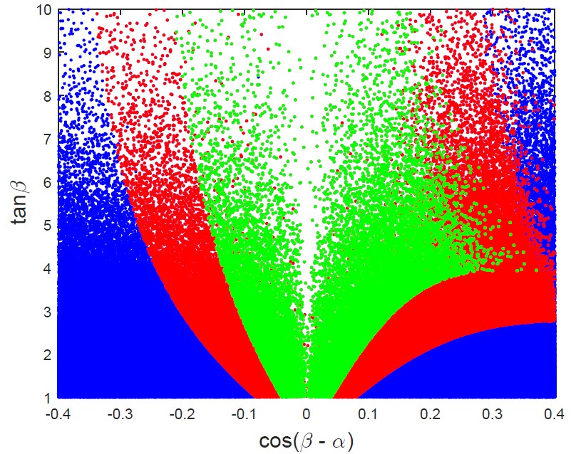
notice that the density of points in this plot has no physical meaning, it is just a consequence of the fact that certain regions of parameter-space are harder to simulate than others (due to the several constraints being imposed, both theoretical and experimental).
We now turn to predictions obtained for the muon-specific model. The ratio of the dimuon coupling of the Higgs to the ditau coupling is, as can be seen from Eqs. 5 and 6, only dependent on and , and given , the range of can be determined from Figure 1. Defining () as the ratio of the dimuon (ditau) coupling of the SM-like Higgs to the Standard Model value, we have, from Eqs. 5 and 6,
| (9) |
If we plot as a function of we obtain Figure 2.
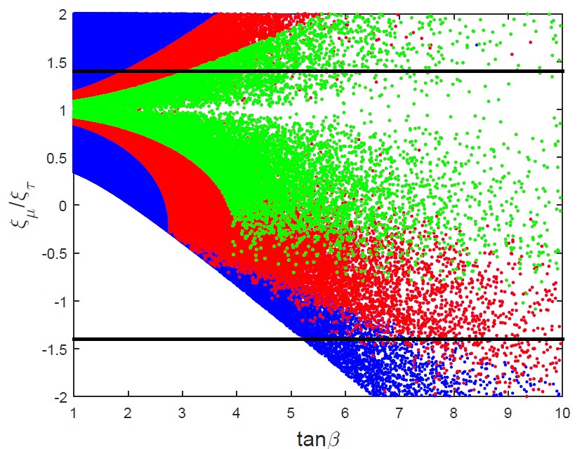
Since the experimental bound on is 1.3 and must be within approximately of unity, the allowed experimental region is between the horizontal lines, corresponding to . One can see that there is a sizeable region in which the dimuon coupling vanishes, as well as a region in which it is enhanced.
As a consequence, the dimuon production rate for the 125 GeV neutral scalar can be substantially suppressed or enhanced. In Figure 3 we show the quantity (defined in Eq. 8 for the final state ) as a function of . Having would mean that the dimuon decay of the would behave exactly like the SM Higgs.
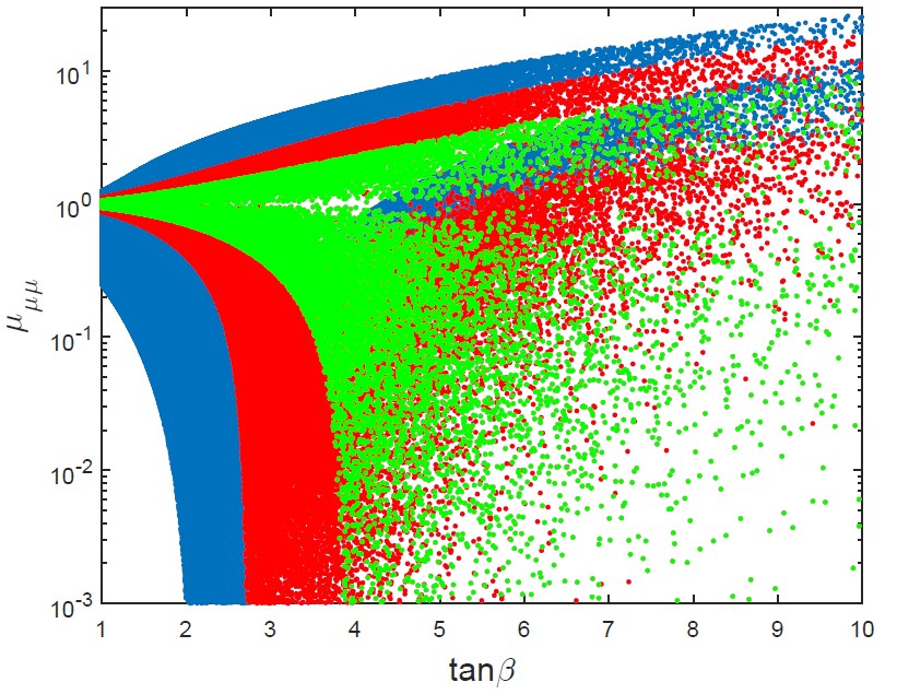
As we see, it is easy to suppress the muon rate to a point where it will never be observed at the LHC in the muon-specific model – but it is also possible to accommodate a muon rate significantly larger than the SM expectation.
Since , and depend only on and , any two will determine the third. The relation (first noted in Ref. [17]) is
| (10) |
This is undefined at , but at that precise point, , so and thus . Since we know that is approximately 1, can be written as . Expanding in powers of , one finds
| (11) | |||||
| (12) | |||||
| (13) |
Note that can have either sign. The fact that is experimentally greater than only implies that . We see that for moderately large , one can easily suppress the dimuon decay substantially. In principle, measurements of and would thus determine , but given that the uncertainty in these measurements will be at least a few percent for decades, it will be difficult to be precise. Note that the model does predict that if the dimuon coupling is suppressed, then the ditau coupling will be enhanced.
4.2 Charged Higgs phenomenology
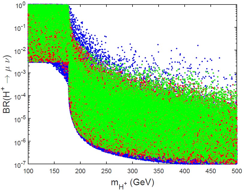
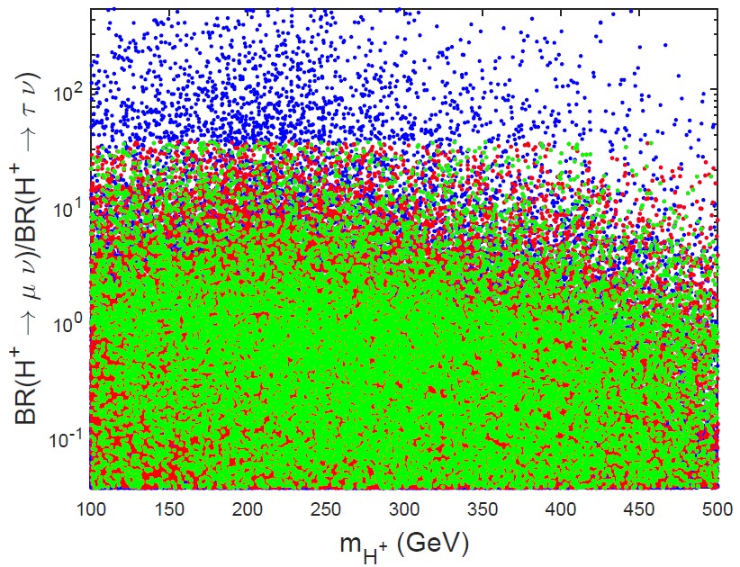
The charged Higgs can have a completely different phenomenology from that of a Type I model, since its dominant decay will, for a range of masses and choices of , be , instead of the usual decays into taus. In fact, as can be appreciated from Figure 4, the charged Higgs branching ratio to muon leptons can be close to unity for a very large range of parameters; and can be substantially larger than that for tau leptons, even with 125 GeV Higgs rates very close to their SM expectations.
 |
 |
| (a) | (b) |
The larger values of BR are clearly obtained for masses of the charged Higgs inferior to GeV – above that mass, the decay channel opens up and becomes dominant. In fact, if one requires the muon decay of the charged Higgs to be dominant, one is left with a narrow range of masses for which that would be possible. In Figure 5 we show the charged Higgs production cross section as a function of the scalar mass for a choice of parameters such that the branching ratio of is . In this case, the muon channel would presumably be the best discovery channel for the charged Higgs. For this figure we restricted ourselves to points
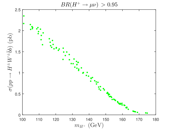
for which the 125 GeV neutral scalar has values of the ratios within 10% of SM values, and such that , that is, the current LHC bound for muon decays of . The main production process for a charged Higgs in this mass range is via production of a top pair, one of the top quarks decaying to and the other to . The numbers for the LHC, 13 TeV, cross section were obtained from [22], duly scaled by appropriate factors of . Notice that this region of interest – SM-like muon interactions for , but a subversion of the expectations for the charged Higgs phenomenology, with a dominant muon decay channel – only occurs for values of the charged mass below 180 GeV, which justifies the choice of quark-Higgs couplings akin to Type I’s. One could also choose Type-II-like quark couplings with appropriate choice of quantum numbers, but constraints would automatically force the charged mass to be above roughly 580 GeV [23, 24, 25, 26, 27, 28]. Also of note is the fact that the parameter space points represented in Figure 5 occur for a narrow range of values of , namely between 8.97 and 9.92, which makes them safe from the -physics constraints affecting smaller masses of the charged scalar for a Type-I 2HDM [28].
Finally, one may wonder if the region of parameter space where muonic decays of the charged scalar are enhanced implies a similar enhancement of the muon branching ratio of . We see, in Figure 6, that this is not so: the region where the largest values of
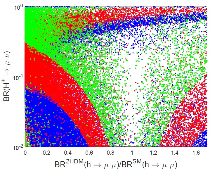
BR occur (even for a scalar with non-muon production and decay rates within 10% of SM expectations) can in fact occur when the muonic decays of are highly suppressed – but also, though less likely, when they are enhanced. The explanation, once more, may be found in the structure of the muonic Yukawa couplings shown in Eqs. 5–7. We see from the latter equation that the muon interactions of the charged scalar are enhanced for high values of , which simultaneously decreases the tau ones – thus the branching ratio BR will become dominant for high (and low enough mass of the charged, see discussion above for Figure 4). And if is of the order of then the muonic decays of will be highly suppressed, as seen in Eq. 6. Larger still , however, may actually lead to an enhancement of the magnitude of ’s muonic Yukawa coupling (though with the opposite sign from the SM expectation). A final observation – in Figure 6 we only include values of BR smaller than 1.7 times the SM Higgs muonic branching ratio, given that that is the current upper bound for that quantity stemming from LHC results.
4.3 Heavier neutral scalars
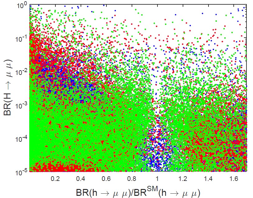
We now consider the heavy neutral scalars in the model. As for and , we are interested in the muon interactions of the heavier CP-even scalar and the pseudoscalar , so we show, in Figure 7, the dimuon branching ratios of both and as a function of
 |
 |
| (a) | (b) |
the muonic branching ratio of the SM-like Higgs (normalized to the expected SM value). We observe that it is possible to find regions of parameter space for which the muonic decays of both and are enhanced and can even become dominant – it is easier to accomplish this for the pseudoscalar since its fermionic couplings are independent of (whereas for there is a tendency to have Yukawa couplings suppressed in the regions where has SM-like interactions, see Eqs. 5–6). We see then that there are regions of parameter space for which the decays into muons can become the main decay channel, raising the possibility of a discovery of these extra scalars by analysing muon pairs produced at the LHC. In Figure 8 we show the signal strength for the production of a pseudoscalar via gluon-gluon fusion at the LHC at 13 TeV, and its subsequent decay into muon pairs. We chose a region of parameter space for which the SM-like has production and decay rates within 10% of the SM expectation, as explained before; and for which the muonic branching ratio of is superior to 50%. This choice of points includes suppressed muonic couplings, but also points for which the SM-like muonic couplings are enhanced. Unlike the charged Higgs situation, it is not possible to find a region where has rates within 10% of SM values and BR – the maximum value of this branching ratio for this chosen parameter space is 0.75, though that would have increased had our scan included larger values of (the points shown in Figure 8 have values of in the range between 7.7 and 10). And as occurred for the charged Higgs, only pseudoscalars with lower masses (below 210 GeV) would have a phenomenology marked by large muonic branching ratios.
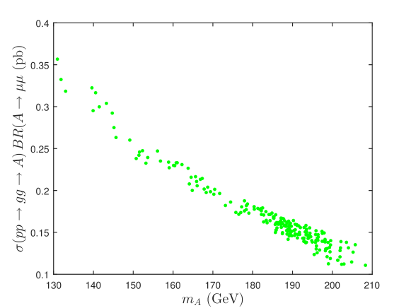
Of course, there are many mechanisms for muon pair production at the LHC, and the magnitude of the signal associated with this pseudoscalar decaying to muons (roughly between 0.1 and 0.4 pb) would likely be drowned in backgrounds.
A similar exercise could be done for the heavier CP-even scalar , but the results are less interesting: the region of parameter space for which: (a) has signal rates within 10% of its SM values; (b) its muonic branching ratio is smaller than 1.7 times its SM value; and (c) BR is dominant, occurs for masses between 130 and 165 GeV. The maximum value of the muonic branching ratio of is found to be roughly 0.78, and one obtains pb, which is even less likely to lead to discovery than the pseudoscalar case.
4.4 Di-Higgs production
As noted in the last subsection, backgrounds involving muon pairs can be quite severe. One can consider di-Higgs production, through or . These would lead to spectacular three and four muon events for which the backgrounds would be much smaller. Note that the dimuon decays of the charged and neutral Higgs are dominant only for a small range of masses (roughly between 100 and 200 GeV), as shown in the previous subsections, and these three and four muon events require that both scalars are in this small range. Nonetheless, the possibility should be discussed. Assuming that both scalars are produced on-shell, we can use the results from the 2HDM Benchmark LHC Working Group for the Inert Doublet Model (IDM)– specifically, their Benchmark Point 5, BP5, results [29] (see also [30, 31, 32]) – to obtain diHiggs production cross sections. Given the form of the vertices , and within the 2HDM, we have 333Obviously, if the 2HDM considered was the IDM, we would simply use . that the production cross sections for and are times the same processes in the IDM, and the production cross section for is the same as in the IDM.
We wish to ascertain whether in the context of the muon-specific model, where the extra scalars may have very large muonic decay branching ratios, one can have a very clear 3– or 4–muon signal. With this in mind, let us provide two benchmark points (BP) to illustrate the best-case scenario within the model. We require that the 125 GeV neutral scalar has values of the ratios within 10% of SM values, and that (the current LHC bound for muon decays of ). With such constraints, we then choose the following BPs:
-
•
BP1, Maximal neutral muonic branching ratios: we choose parameters to maximize the product . This will yield the maximal 4–muon signal.
-
•
BP2, Maximal charged-neutral muonic branching ratios: we choose parameters to maximize the product . This will yield the maximal 3–muon signal.
Investigating our parameter scan detailed in the previous subsections, we find the parameters for each BP as presented in table 1.
| Parameters | Benchmark Point 1 | Benchmark Point 2 |
|---|---|---|
| (GeV) | 130.9 | 141.2 |
| (GeV) | 115.2 | 149.6 |
| (GeV) | 152.0 | 161.3 |
| 9.2 | 9.4 | |
| 0.993 | 0.997 | |
| (GeV2) | 1382.9 | 2008.4 |
We can then read off from the BP5 plots in [29] the rough values for the 13 TeV LHC cross sections for dihiggs production. For instance, for BP1 we have pb and for BP2 pb. Computing the muonic branching ratios of the several scalars and reading off the production cross sections we obtain the results in table 2, with the 3–muon signal computed as
| (14) | |||||
and the 4–muon signal given by
| (15) |
| Benchmark Point 1 | Benchmark Point 2 | |
|---|---|---|
| 0.77 | 0.74 | |
| 0.67 | 0.67 | |
| 0.54 | 0.92 | |
| (pb) | 0.1 | 0.05 |
| (pb) | 0.05 | 0.05 |
| (pb) | 0.04 | 0.04 |
| (pb) | 0.039 | 0.052 |
| (pb) | 0.051 | 0.0248 |
As before, larger values for and would be obtained for larger values of – for instance, for , GeV and GeV, one would obtain and for , GeV, GeV and GeV, one would obtain .
These cross sections are of the order of tens of femtobarns. There are many analyses of multiple muon events at the LHC in the context of very light scalars, where the scalars are relativistic and thus the muon pairs are collimated (“muon jets”). Here the scalars are not highly relativistic, and thus the opening angle of the muon pairs will be large. It is possible that a detailed analysis of these processes could exclude some of the model’s parameter space, in which both of the heavy scalars are within the to GeV range.
5 Conclusions
The current experimental value of the dimuon decay of the Higgs boson is times the Standard Model expectation. In this paper, we have questioned the implications of a future result in which this decay is substantially suppressed. Since the ditau decay is close to the Standard Model expectation, this would mean that the muon and tau must couple to different scalar bosons. In most such models, this results in dangerous tree-level flavor-changing neutral currents, however such currents are avoided in the ASY “muon-specific” 2HDM. The original ASY analysis hoped to explain the g-2 anomaly, but this requires a high degree of fine-tuning. Here, we abandon attempting to explain the g-2 anomaly, and study the phenomenological implications of the model.
We first study the decays of the 125 GeV Higgs boson. It is shown that there is a wide range of parameters in which the dimuon decay rate can be suppressed, even eliminated, without affecting the other decays. The ASY model predicts a relationship between the ZZ, ditau and dimuon decays that can eventually be tested, although sufficient precision will almost certainly require a Higgs factory. The relation shows that a substantial suppression in the dimuon rate does lead to a very small increase in the ditau rate.
Since the model is, for all fermions but the muon, close to a type I 2HDM, bounds on charged Higgs masses are not strong. For masses below about 175 GeV, we show that the decay can dominate the charged Higgs decays, leading to a very different phenomenology. Above 175 GeV, the decay becomes accessible and indeed dominant, but for lower masses the muonic decay can dominate over the tau decay. For the heavy neutral scalars, one can find substantial regions of parameter space in which the dimuon decay dominates, especially for the pseudoscalar Higgs. This also occurs for fairly light masses. These decays, given the large number of muon pairs at the LHC, may be swamped by other processes. On the other hand, if two of the heavy scalars are in a similar mass range, then multimuon events could provide a distinctive signature.
One could imagine using the same mechanism of the ASY model in the quark sector, to enhance or suppress couplings of to the second or first generation of quarks, the measurements of which have not yet been achieved. One could imagine that probing the Higgs-charm coupling might be possible indirectly, via interference effects in the gluon-gluon fusion cross section, or in the diphoton decay width. A strong enhancement of the coupling of to charm quarks (a “charming Higgs”) could then be ruled out. Likewise one could suppress this coupling ( “charmless Higgs”), though the exclusion of that possibility seems unlikely within the expected lifetime of the LHC. Similar ideas could be explored vis-a-vis couplings of to , or quarks. One might even consider enhancing/suppressing the third generation quark couplings, if increased precision in their measurements showed deviations unable to be reproduced by regular 2HDMs. However, the ASY mechanism runs into a serious obstacle if one tries to extend it to the quark sector – since it would require that for a given generation one of the quark left doublets and the corresponding quark right singlet transform differently from the other two generations, attempting to reproducing the ASY mechanism in the quark sector would result in an unphysical CKM matrix – namely, one would find that the CKM matrix would be block diagonal, thus contradicting experimental confirmation of all its elements being non-zero. This conundrum might be solved with a more complicated scalar and/or quark sector, but that goes beyond the scope of the current work.
Acknowledgments
PF is supported in part by a CERN grant CERN/FIS-PAR/0002/2017, an FCT grant PTDC/FIS-PAR/31000/2017, by the CFTC-UL strategic project UID/FIS/00618/2019 and by the NSC, Poland, HARMONIA UMO-2015/18/M/ST2/00518. The work of MS was supported by the National Science Foundation under Grant PHY-1819575. We thank Igor Ivanov for clarifying the symmetry group of the model.
References
- [1] G. Aad et al. [ATLAS Collaboration], Phys. Lett. B 716 (2012) 1 doi:10.1016/j.physletb.2012.08.020 [arXiv:1207.7214 [hep-ex]].
- [2] S. Chatrchyan et al. [CMS Collaboration], Phys. Lett. B 716 (2012) 30 doi:10.1016/j.physletb.2012.08.021 [arXiv:1207.7235 [hep-ex]].
- [3] G. Aad et al. [ATLAS Collaboration], JHEP 1504 (2015) 117 doi:10.1007/JHEP04(2015)117 [arXiv:1501.04943 [hep-ex]].
- [4] S. Chatrchyan et al. [CMS Collaboration], JHEP 1405 (2014 ) 104 doi:10.1007/JHEP05(2014)104 [arXiv:1401.5041 [hep-ex]].
- [5] M. Aaboud et al. [ATLAS Collaboration], Phys. Lett. B 786 (2018) 59 doi:10.1016/j.physletb.2018.09.013 [arXiv:1808.08238 [hep-ex]].
- [6] A. M. Sirunyan et al. [CMS Collaboration], Phys. Rev. Lett. 121 (2018) no.12, 121801 doi:10.1103/PhysRevLett.121.121801 [arXiv:1808.08242 [hep-ex]].
- [7] A. M. Sirunyan et al. [CMS Collaboration], Phys. Rev. Lett. 120 (2018) no.23, 231801 doi:10.1103/PhysRevLett.120.231801 [arXiv:1804.02610 [hep-ex]].
- [8] M. Aaboud et al. [ATLAS Collaboration], Phys. Lett. B 784 (2018) 173 doi:10.1016/j.physletb.2018.07.035 [arXiv:1806.00425 [hep-ex]].
- [9] A. M. Sirunyan et al. [CMS Collaboration], Phys. Rev. Lett. 122 (2019) no.2, 021801 doi:10.1103/PhysRevLett.122.021801 [arXiv:1807.06325 [hep-ex]].
- [10] The ATLAS collaboration [ATLAS Collaboration], ATLAS-CONF-2019-028.
- [11] F. J. Botella, G. C. Branco, M. N. Rebelo and J. I. Silva-Marcos, Phys. Rev. D 94 (2016) no.11, 115031 doi:10.1103/PhysRevD.94.115031 [arXiv:1602.08011 [hep-ph]].
- [12] G. C. Branco, W. Grimus and L. Lavoura, Phys. Lett. B 380 (1996) 119 doi:10.1016/0370-2693(96)00494-7 [hep-ph/9601383].
- [13] F. J. Botella, G. C. Branco and M. N. Rebelo, Phys. Lett. B 687 (2010) 194 doi:10.1016/j.physletb.2010.03.014 [arXiv:0911.1753 [hep-ph]].
- [14] T. Abe, R. Sato and K. Yagyu, JHEP 1707, 012 (2017) doi:10.1007/JHEP07(2017)012 [arXiv:1705.01469 [hep-ph]].
- [15] I. P. Ivanov and C. C. Nishi, JHEP 1311, 069 (2013) doi:10.1007/JHEP11(2013)069 [arXiv:1309.3682 [hep-ph]].
- [16] G. C. Branco, P. M. Ferreira, L. Lavoura, M. N. Rebelo, M. Sher and J. P. Silva, Phys. Rept. 516 (2012) 1 doi:10.1016/j.physrep.2012.02.002 [arXiv:1106.0034 [hep-ph]].
- [17] A. Dery, C. Frugiuele and Y. Nir, JHEP 1804 (2018) 044 doi:10.1007/JHEP04(2018)044 [arXiv:1712.04514 [hep-ph]].
- [18] P. M. Ferreira, R. Santos, M. Sher and J. P. Silva, Phys. Rev. D 85, 035020 (2012) doi:10.1103/PhysRevD.85.035020 [arXiv:1201.0019 [hep-ph]].
- [19] T. Biek tter, M. Chakraborti and S. Heinemeyer, Eur. Phys. J. C 80, no. 1, 2 (2020) doi:10.1140/epjc/s10052-019-7561-2 [arXiv:1903.11661 [hep-ph]].
- [20] R. V. Harlander, S. Liebler and H. Mantler, Comput. Phys. Commun. 184, 1605 (2013) doi:10.1016/j.cpc.2013.02.006 [arXiv:1212.3249 [hep-ph]].
- [21] R. V. Harlander, S. Liebler and H. Mantler, Comput. Phys. Commun. 212, 239 (2017) doi:10.1016/j.cpc.2016.10.015 [arXiv:1605.03190 [hep-ph]].
- [22] C. Degrande, R. Frederix, V. Hirschi, M. Ubiali, M. Wiesemann and M. Zaro, Phys. Lett. B 772, 87 (2017) doi:10.1016/j.physletb.2017.06.037 [arXiv:1607.05291 [hep-ph]].
- [23] O. Deschamps, S. Descotes-Genon, S. Monteil, V. Niess, S. T’Jampens and V. Tisserand, Phys. Rev. D 82, 073012 (2010) doi:10.1103/PhysRevD.82.073012 [arXiv:0907.5135 [hep-ph]].
- [24] F. Mahmoudi and O. Stal, Phys. Rev. D 81, 035016 (2010) doi:10.1103/PhysRevD.81.035016 [arXiv:0907.1791 [hep-ph]].
- [25] T. Hermann, M. Misiak and M. Steinhauser, JHEP 1211, 036 (2012) doi:10.1007/JHEP11(2012)036 [arXiv:1208.2788 [hep-ph]].
- [26] M. Misiak et al., Phys. Rev. Lett. 114, no. 22, 221801 (2015) doi:10.1103/PhysRevLett.114.221801 [arXiv:1503.01789 [hep-ph]].
- [27] M. Misiak and M. Steinhauser, Eur. Phys. J. C 77, no. 3, 201 (2017) doi:10.1140/epjc/s10052-017-4776-y [arXiv:1702.04571 [hep-ph]].
- [28] J. Haller, A. Hoecker, R. Kogler, K. M nig, T. Peiffer and J. Stelzer, Eur. Phys. J. C 78, no. 8, 675 (2018) doi:10.1140/epjc/s10052-018-6131-3 [arXiv:1803.01853 [hep-ph]].
- [29] A. Ilnicka, M. Krawczyk, D. Sokolowska and T. Robens, Benchmark Point 5 in https://twiki.cern.ch/twiki/bin/view/LHCPhysics/LHCHXSWG3Benchmarks2HDM.
- [30] A. Ilnicka, M. Krawczyk and T. Robens, Phys. Rev. D 93, no. 5, 055026 (2016) doi:10.1103/PhysRevD.93.055026 [arXiv:1508.01671 [hep-ph]].
- [31] D. de Florian et al. [LHC Higgs Cross Section Working Group], doi:10.2172/1345634, 10.23731/CYRM-2017-002 arXiv:1610.07922 [hep-ph].
- [32] J. Kalinowski, W. Kotlarski, T. Robens, D. Sokolowska and A. F. Zarnecki, JHEP 1812, 081 (2018) doi:10.1007/JHEP12(2018)081 [arXiv:1809.07712 [hep-ph]].