Pinning of interfaces in a random medium with zero mean
Abstract
We consider two related models for the propagation of a curvature sensitive interface in a time independent random medium. In both cases we suppose that the medium contains obstacles that act on the propagation of the interface with an inhibitory or an acceleratory force. We show that the interface remains bounded for all times even when a small constant external driving force is applied. This phenomenon has already been known when only inhibitory obstacles are present. In this work we extend this result to the case of—for example—a random medium of random zero mean forcing.
The first model we study is discrete with a random forcing on each lattice site. In this case we construct a supersolution employing a local path optimization procedure. In the second, continuous, model we consider a random heterogenous medium consisting of localized small obstacles of random sign. To construct a stationary supersolution here, we need to pass through sufficiently many blocking obstacles while avoiding any obstacles of the other sign. This is done by employing a custom percolation argument.
2020 Mathematics Subject Classification. 35R60, 74N20.
Key words and phrases. Quenched Edwards-Wilkinson model, phase boundaries, pinning, random environment, viscosity super-solutions
1 Introduction
We are investigating a model for an interface propagating through a random, heterogeneous medium. As a governing equation, we consider
| (1) |
This equation arises for example as a linearization of the mean curvature flow with a spatially non-homogeneous driving force (see, e.g., [6, 5] for a derivation). The graph of is the shape of the interface at time , is a given exterior driving force and is the force exerted by the medium on the interface. The function is supposed to be non-zero only in small sets which correspond, for example, to obstacles, impurities or precipitates in the medium. Such a setting is commonly found when studying magnetic domain values, dislocation lines, or charge density waves. For a more detailed list of related problems and applications, we refer to [2, 6].
In the deterministic, periodic setting this problem was studied in [6], with having zero mean (or at least this being a sufficient condition for their results). The authors show that in this case, under some non-degeneracy conditions, there exists a critical driving force , up to which pinning occurs, i.e., the evolving interface stays below some stationary hypersurface for all times. For larger driving forces, there is a non-stationary solution to the problem that propagates with positive average velocity.
Here, we consider a random setting, which can be seen as a variant of the quenched Edwards-Wilkinson model, in the sense that the strengths and positions of obstacles are random and non-correlated on long distances, but time-independent. Furthermore, they may act on the interface in both directions (i.e., is not assumed to be non-negative). Thus, our model also includes the case with random forces having zero mean, which is a common setting in the physics literature, see, e.g., [2, 13].
Our goal is to show a result regarding pinning for two models. In both models we consider only the one dimensional case, so that the interface is in fact a curve, and our equation reads
where exceptionally we stressed the randomness of the setting given by a probability space by writing the random variable . The interface is initially supposed to be flat having the height 0, i.e. . The basic idea is to a.s. find a (viscosity) supersolution (for the definition and properties see, e.g., [3]) to the related stationary problem, i.e., a function that satisfies
By employing an appropriate comparison principle, this immediately implies that the interface a.s. stays below the graph of for all times since this was the case at . Our main goal in this work is thus to show the existence of such a non-negative stationary supersolution in the setting of our two models.
The first model we study is spatially purely discrete; we there consider the lattice . Each lattice point acts with a force of random strength chosen by a suitable probability distribution. The notions of the space and time derivative are adapted to the discrete case. This model was studied in, e.g., [1], where for some very specific distributions of pinning and depinning results were shown. Here, we focus on results regarding pinning, but consider a large class of distributions (in particular, allowing the aforementioned case of having zero mean).
For the continuous setting, for the case , the occurrence of pinning for sufficiently small driving force was shown in [5]. Depinning results for unbounded obstacles were studied, e.g., in [7, 8]. To prove pinning results in the case of obstacles without prescribed sign, we follow a similar strategy of localization and percolation as [5], but require a more explicit form of the constructed supersolution. This is possible due to our one-dimensional setting. Moreover, it is necessary to extend the percolation result from [4] to the case with finite dependence of sites.
2 Discrete model on
Let the obstacle strenghts , be independent and identically distributed -valued random variables defined on a probability space . We denote the expected value of a (possibly extended real-valued) random variable on that space by (whenever it is defined). We consider the following continuous time evolution of (random) functions , . The initial condition is . The function can jump from its current value to or to depending on the value of and the discrete Laplacian defined as
The corresponding jump rate is with the interpretation that if , then can only jump to (with rate ) and when , then can only jump to and does so with rate . Here, is a strictly increasing function from to which satisfies . The phrase jumps from to with rate means - as usual - that for some exponentially distributed random variable with parameter which is independent of the field , for all , where is the first time after when the Laplacian at changes (due to a jump of one of the neighbors) and where in case .
One may ask under which conditions on as above there exists a unique process with values in the functions from to associated to the given rates. This clearly holds when is bounded which we can safely assume since none of the following results in this section depends on (except for its sign).
Let be independent random variables which have the same distribution as .
Theorem 2.1.
If
then, almost surely, there exists a function such that , i.e., a non-negative supersolution.
Proof.
Without loss of generality we can and will assume that is essentially bounded from above. We first construct a supersolution and show that it is almost surely bounded from below. Then the claim will follow easily.
We start by defining . Fix , and let be the smallest integer for which and . The condition in the theorem guarantees that such an exists. Let . We will successively construct from the previous values and the obstacle strengths , (the construction for negative values is completely analogous). We will always first define a provisional value which we will then (possibly) change to the smaller final value depending on the obstacles , . We will perform the construction in such a way that the sequence satisfies the condition of a supersolution at . Note that when we later change to a smaller value then this property still holds for the sequence .
We define the provisional values in such a way that the sequence , , satisfies the condition of a supersolution at 0. Specifically, we choose .
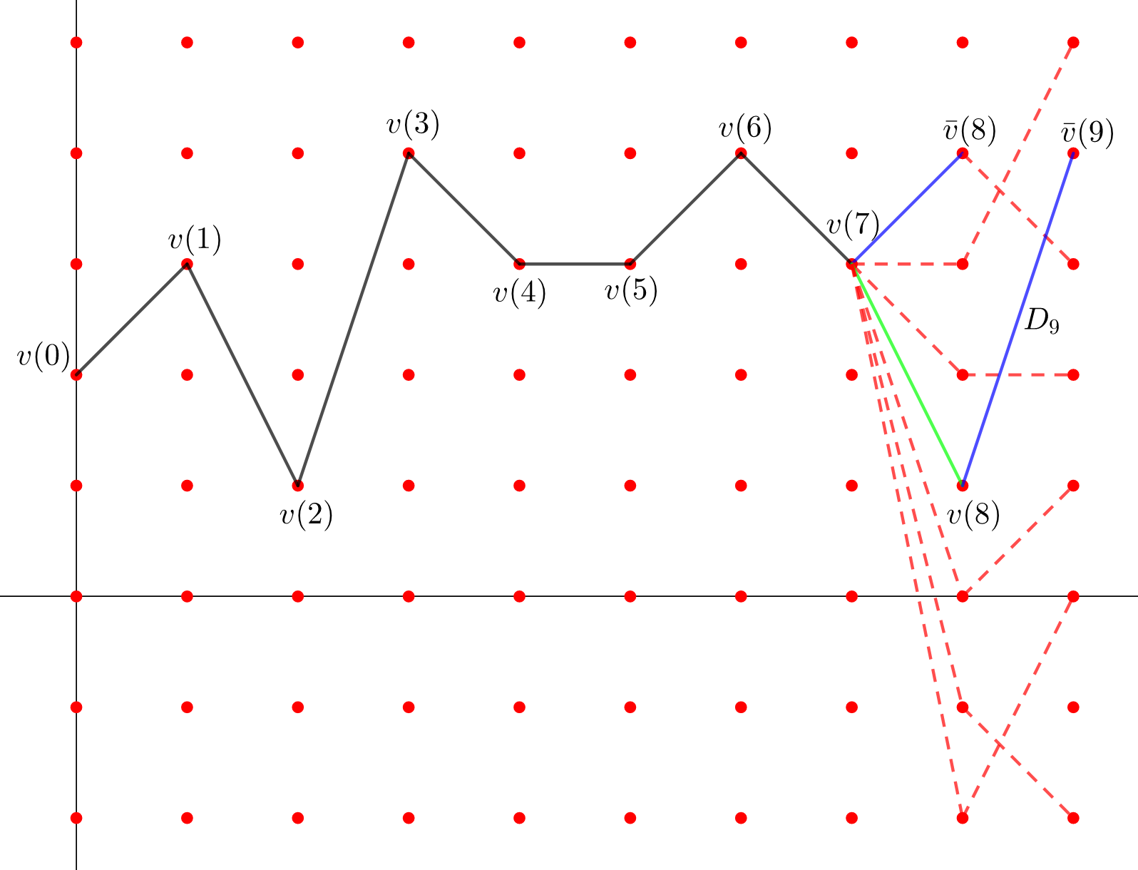
Given and for some , we now define and in such a way that the increment is as large as possible subject to the conditions and the supersolution condition at . The idea behind this choice is that large increments are likely to ensure that is bounded from below. Clearly, the optimal choices are where maximizes and (which satisfies the supersolution condition at with equality). Note that a maximizing exists since is essentially bounded from above. For an illustration of this procedure, see Figure 1 below.
Note that the sequence , is a supersolution by construction. We check that the function is almost surely bounded from below.
Define . By construction (and our independence assumptions) the random variables , are independent and identically distributed with expectation
(Note that independence of the increments is generally lost if we delete the bar in the definition of .) We have, for ,
Note that the sequence , is i.i.d. with expected value larger than which implies almost surely. Further, by the strong law of large numbers, almost surely. Hence,
converges to almost surely. In particular, for all sufficiently large (and, analogously, for all sufficiently large ). In particular, the function is almost surely bounded from below. Using translation invariance, we see that the probability that the function is non-negative converges to 1 as the initially chosen converges to , i.e. we have proven the almost sure existence of a non-negative supersolution. ∎
Remark 2.2.
In the special case , the condition in the theorem holds iff .
Corollary 2.3.
If, for some ,
then, almost surely, there exists a function such that .
3 Continuum model
3.1 Setting
In the continuum setting of equation (1), we consider to be of the form
| (2) |
where is a 2-dimensional Poisson point process prescribing the centers of the obstacles. The random variables , which are assumed to be identically distributed and independent of the obstacle centers, prescribe the strength of each individual obstacle and must satisfy for some .
In order to prove our result, we have to introduce a small parameter which determines the spatial extent of the obstacles, and will be chosen according to the statistical parameters of the obstacle distribution. Therefore, we assume that the function satisfies and for some . As one can read off (2), this implies that the obstacles achieve their full strength on a square of side-length and vanish outside a ball of radius . Since small obstacles have a small effect on the propagating interface, we rescale their force by such that their effect remains constant when changing . It will turn out that the choice is suitable.
Such an assumption of very small obstacles is also made in [11], where point obstacles are considered in a model for dislocation evolution. Their assumptions can be interpreted as the limit of our model.
Again, we will show a.s. existence of a non-negative viscosity supersolution of
| (3) |
The function , that we construct, will be piecewise quadratic, and in points of non-differentiability the condition on viscosity solution will be trivially met, as from our construction it will hold that
To simplify this construction, we will work with the following setting. We split the obstacles into those with (and refer to them as positive) and into those with (negative). Obstacles for which will be ignored. The centers of the positive/negative obstacles are now distributed according to independent Poisson point processes on with parameters . Then all positive obstacles have full strength of at least in the squares of side-length centered at . We refer to these squares as cores of the obstacles and denote .
The response of the medium to a given interface may thus be estimated by
dropping the dependence on for notational convenience.
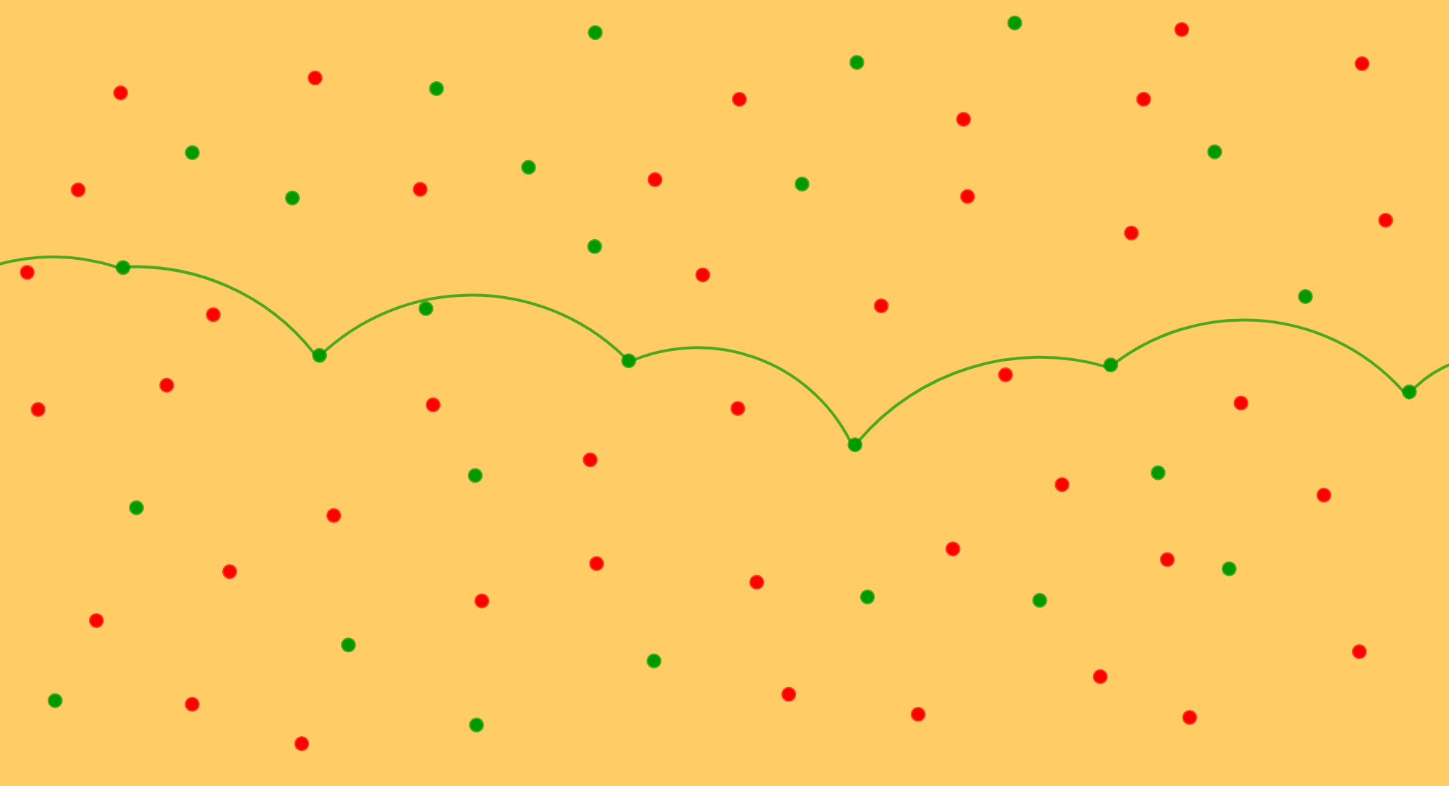
In fact, as shown in Figure 2, we will construct a supersolution that will completely avoid negative obstacles. Therefore, their precise strength does not matter. As for the positive obstacles, we will only employ that they exert force (at least) in the square of size .
3.2 Localization
First we have to localize enough positive obstacles to construct a blocking supersolution. Therefore, let us define
| (4) |
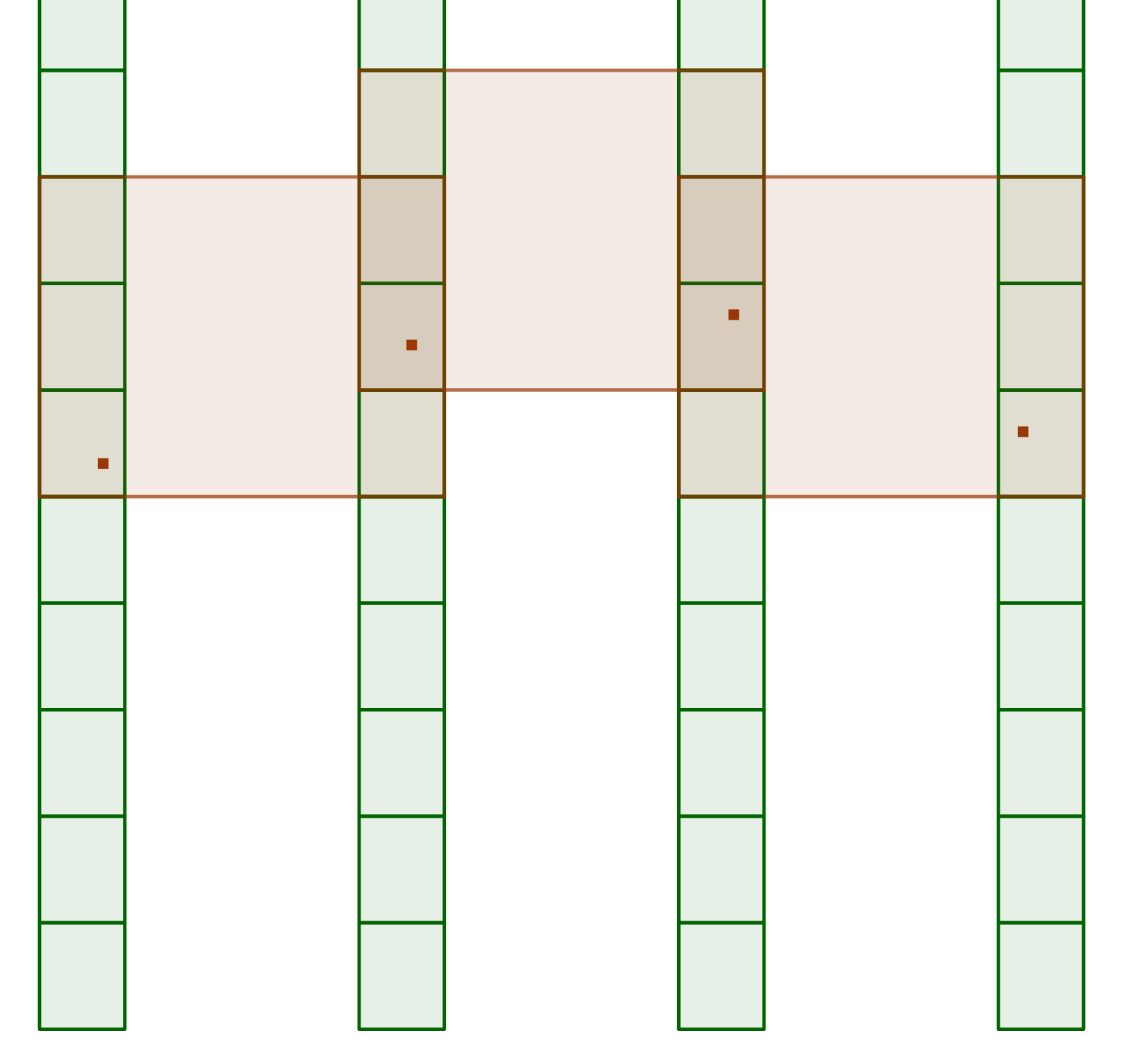
We will consider the obstacles with entire cores lying in one of . As depicted in Figure 3, we thus have columns of rectangles with length and height , and between them there is a free space of width .
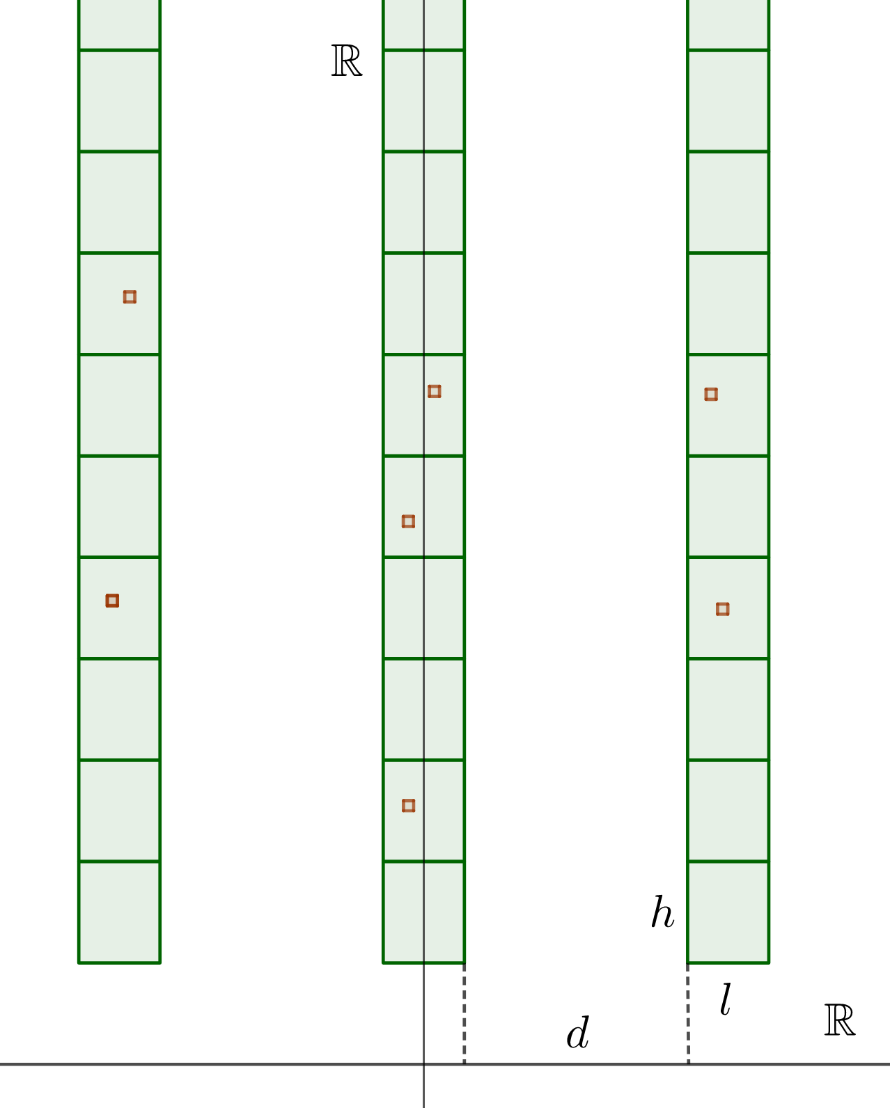
For now, these scales are still completely free. We start at the height so that there is no intersection of the localized positive obstacles with the -axis as long as .
3.3 Inside a core
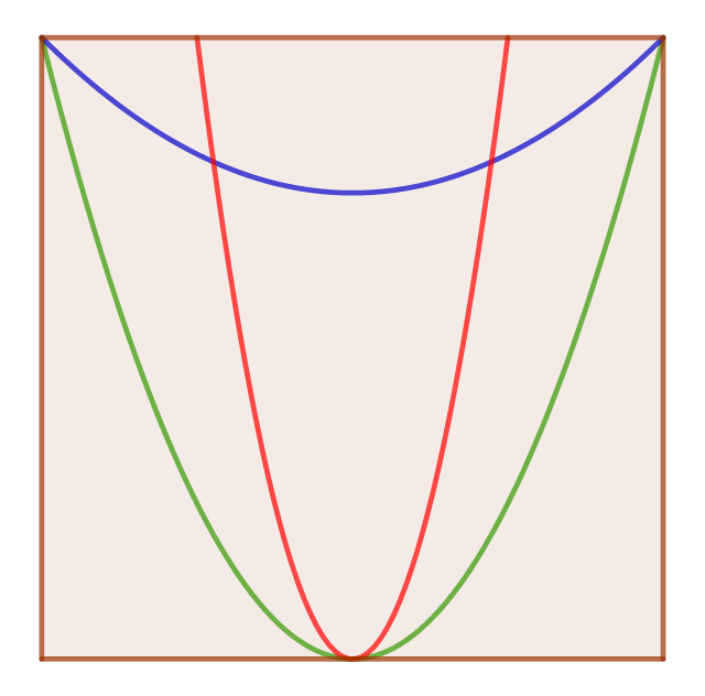
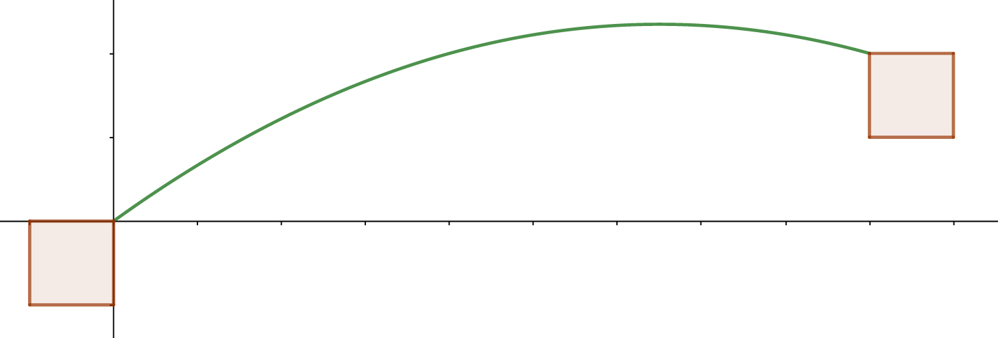
Within the core of a positive obstacle, a sufficient condition to fulfil (3) reads Let us suppose (since in fact, as we will see, we may only pin ). We take the parabola with that has its vertex on the mid vertical line of the core and goes through the upper corners of the core. Its inclination at the upper corners has modulus , and for its vertex lies within the core, see Figure 4.
3.4 An upper bound on the pinned force
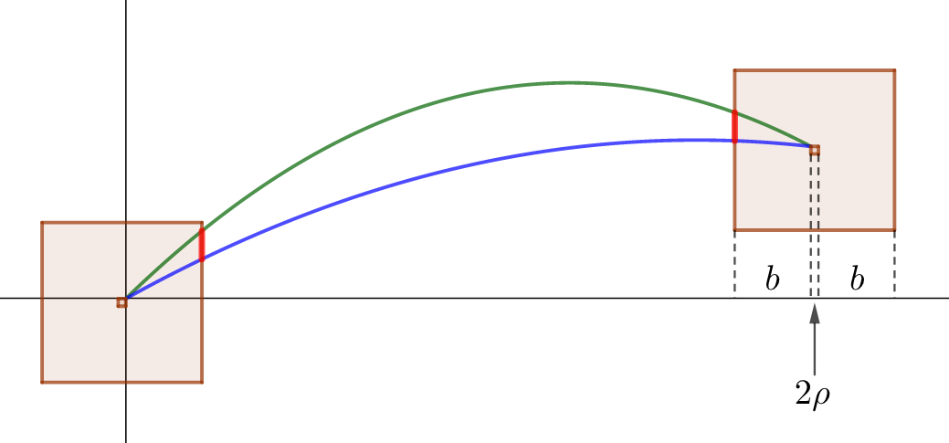
Let us first determine the force that we may block when we have two positive obstacles at a given distance if we suppose that there is no negative obstacle in the vertical strip between them. The exiting points are, as specified in the previous section, the right resp. left corner. Let their positions for the sake of simplicity be and with .
The conditions read
| (5) |
with the latter two ensuring that this function together with the parabolas in the cores forms a supersolution in the viscosity sense. Hence, necessary conditions for existence of a supersolution through the points and are
In the other direction, let and . Then the parabola
is a supersolution between and since and
Conclusion 3.1.
Having two obstacles that produce an exiting inclination with horizontal distance and vertical , we may pin any force of magnitude
To control both distances, we will consider only parabolas between obstacles from the neighbouring columns whose heights differs at most by one unit. If we thus connect two obstacles in boxes and with , then and . We get a positive force if
| (6) |
We then block at least
| (7) |
3.5 Length of the line between parabolas
We must take care not to intersect any negative obstacle with our supersolution. This we achieve by considering only the positive obstacles that fulfill the following two conditions:
-
•
There are no negative obstacles in the square centered at the center of the obstacle with the side where is a new scale. Hence, we have a strip of thickness around the core as shown in Figure 6.
-
•
There are less than (for now arbitrary) negative obstacles in the whole region where parabolas may lie.
We consider a ray of possible parabolas and assess an admissible size of (negative) obstacles as follows:
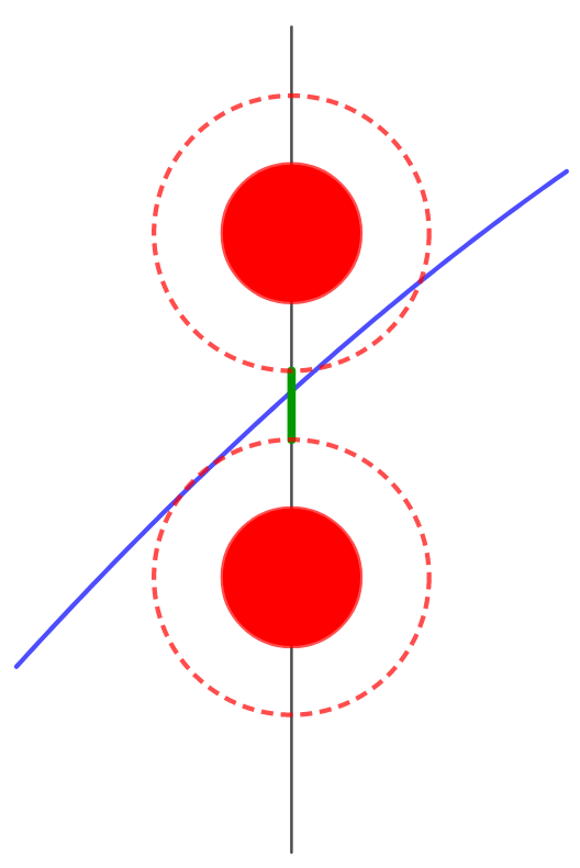
The most problematic position for negative obstacles is on the border of the concentric square (the red line in Figure 6). Suppose all the negative obstacles lie on this line. Then they cover a height up to . We must, however, take into account that parabolas have a certain inclination. If a parabola meets this line outside the balls around the centers of the negative obstacles with radius (the dotted line in Figure 7), then it does not intersect any negative obstacle (lying inside a ball with radius , the red circle in Figure 7), as its inclination surely does not exceed 1. Thus, the negative obstacles block at most . If this length is shorter than the half of the red line, we surely find a parabola around them on both sides.
If a ray of parabolas is given by and with
where then the length of the part of the border of each square determined by this ray is given by
We also notice: Since we restrict ourselves to , that parabolas surely exit the concentric square at the right resp. left side.
3.6 Position of vertex
The parabola
has its vertex in
Since we want to control its height only between and , we have to look at the case . In this case
| (8) |
It suffices to consider . If is too small to fulfil (8), the whole piece of the parabola lies lower than the higher obstacle. Otherwise, let us allow only parabolas with . Since a sufficient condition for this is
| (9) |
For every such , no point of the corresponding parabola between the obstacles lies more than higher than the lower obstacle. Thus, these parabolas surely lie in rectangles of the height depicted in Figure 8.
3.7 Percolation
Now we must obtain a.s. a sequence of “good” rectangles that contain positive obstacles and avoid negative ones such that for all . This can be formulated as a problem in Lipschitz percolation as follows.
Let and consider -independent site percolation on with parameter , i.e. , are random variables taking values in such that for every and , are independent whenever is a subset of for which the following holds: if are elements of , then either or . Note that the case corresponds to the independent site percolation set-up. If , then we say that the site is open and closed otherwise. The last component of plays a different role compared to . We will sometimes call the last coordinate vertical and the others horizontal.
In this set-up the following result holds.
Proposition 3.2.
There is a critical probability such that for every there is a Lipschitz percolation cluster, i.e. almost surely, there exists an open Lipschitz surface, i.e. a function such that whenver and that for all .
Proof.
For this is [4, Theorem 1] or [12, Theorem 1]. In the general case, we will sketch the proof following that of [12, Theorem 1] rather closely.
For each , is its height. Let be the standard basis vectors in .
A -path from to is a finite sequence of distinct states with and such that for every we have
-
•
either , in which case we speak of a step upwards,
-
•
or that is a step downwards.
A -path is called admissible if the endpoint of every step upwards is closed. We denote by the event that there exists an admissible -path from to . As was shown in [12, Section 4], an open Lipschitz surface exists if and only if there exists some such that there does not exist any with and any such that (for a slightly simpler proof [in a slightly more general set-up] avoiding the concept of hills and mountains see [9, 10]). Therefore, we have to show that for sufficiently large and large it is unlikely that there exists an admissible path starting from any point of the form to . Due to a possible lack of translation invariance, we need to modify the proof slightly compared to those mentioned above.
For a -path from to , we denote by and the number of steps upwards resp. downwards. Then and and is admissible if every step upwards ends at a closed site. Due to -independence (and the fact that a -path consists of distinct points) the probability of this happening is at most . Figure 9 shows such an admissible -path. The sites in red must be closed, and we obtain the bound on the probability by realizing that at least of them are independent. In every column, we may simply take the highest one and then every -th one that lies in the path. This bound is also optimal, take, e.g., the straight vertical path .
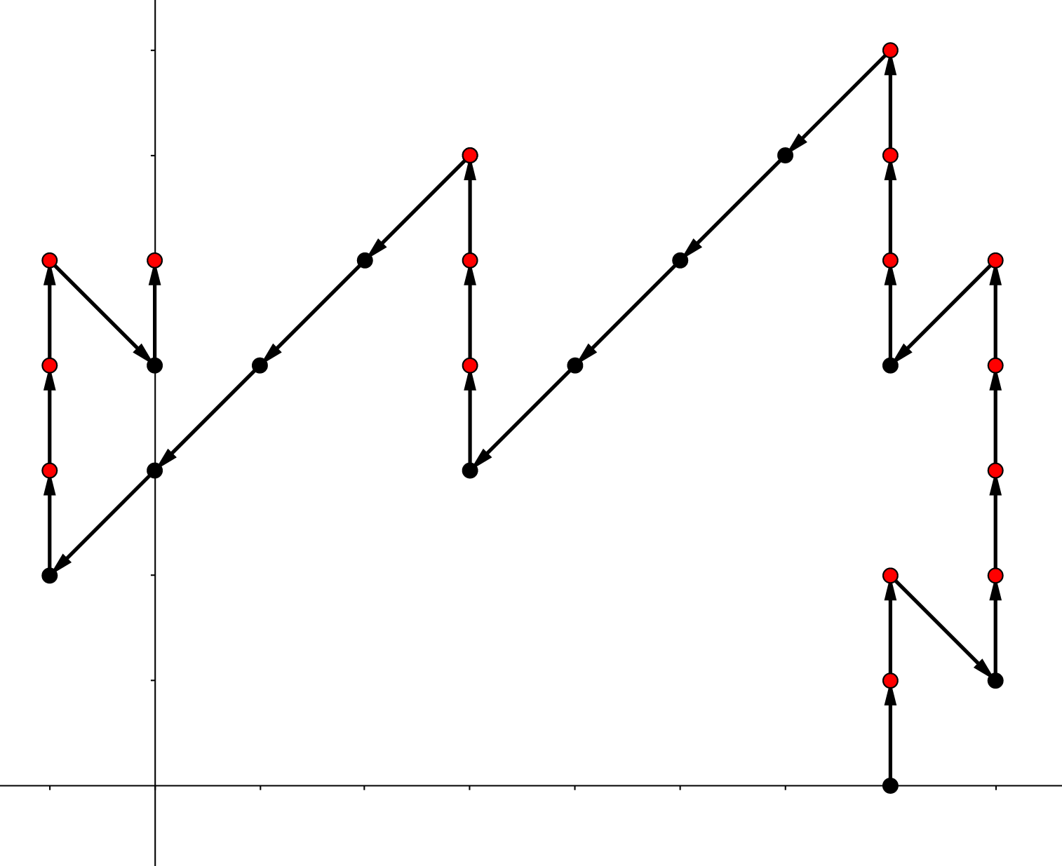
The rest of the proof is as usual (just replacing by ): the expected number of admissible -paths from to is upper bounded by
provided that . In this case the last expression is summable over all and all and the double sum converges to 0 as , so the claim of the proposition follows (with ). ∎
3.8 Putting it together
Now let us state our problem in terms of Lipschitz percolation. Our sites are boxes . We impose three conditions on a box to be open:
-
•
must contain the core of a positive obstacle. Thus we get a condition on the heights and lengths. That means that and that the probability is
-
•
Moreover, a core together with a strip of width around it must not intersect any negative obstacle. We need in order for probabilities to be independent in the horizontal direction and, e.g., to have limited dependence (more precisely, 2-independence) in the vertical direction. The probability then reads
-
•
Lastly, we want the rectangle “around” a positive obstacle with length and height (as in Figure 10) to contain less than centers of negative obstacles. If we denote , then
(If we want the last two events to independent, we may exclude here the square with side . The inequality, however, still holds.)
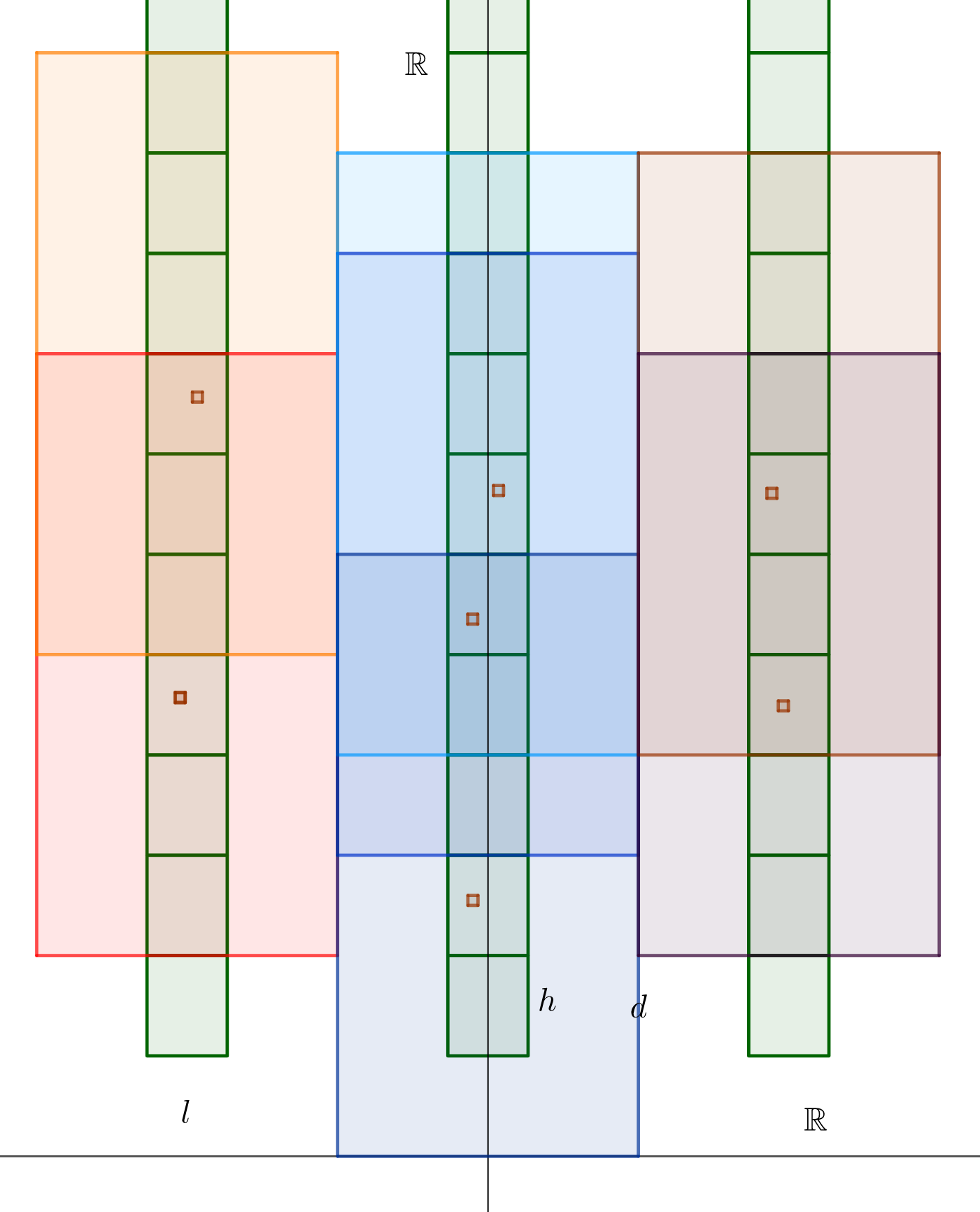
Hence,
We may surely employ Proposition 3.2 if the right-hand side is bigger than since the sites are 6-independent. The scales can be chosen in the following way:
-
(a)
Let us suppose . Set and (to obey (6)), and choose so large that
(10) -
(b)
Suppose We choose small enough so that (thus also ) and
(11) -
(c)
Finally, choose so that
(12)
The percolation result is now applicable, and we get a Lipschitz function between open sites. Each of these open sites contains a positive obstacle, and by (7) and (9), we block by appropriately chosen parabola at least all . Making the choices as above, we arrive at
| (13) |
We choose the interval of admissible forces . The corresponding parabolas cut on the side of the square a line of length
Surely, if
| (14) |
there is a parabola that does not intersect any negative obstacle with center in the two rectangles of size belonging to the open sites. We see that the assumptions on from (a) and (b) are automatically fulfilled. Clearly, we also have , and thus this parabola also cannot intersect any negative obstacle with center outside the rectangles.
Thus, we can show
Theorem 3.3.
Let us suppose the following:
-
•
Distribution: We have two independent Poisson point processes with parameters with , being the corresponding positions of random points.
-
•
Shape: A non-negative function fulfils on and for some .
-
•
Strength: .
Define for every :
Then there exist and such that a.s. there exists a function that satisfies
| (15) |
in the viscosity sense and for all .
Proof.
We choose the scales as described in (10)–(12). Thus we obtain Lipschitz percolating boxes . Then we define
according to (13) and (14). Between two obstacles from adjacent boxes, for some we may a.s. find a parabola that does not intersect any negative obstacle. ( need not be the same for different pairs.)
We define the supersolution in a piecewise manner. Between the cores from the Lipschitz percolating boxes, we take the parabolas from above. Inside the cores, we take parabolas with as described in Subsection 3.3. We notice that the assumption made there is fulfilled. Moreover, the cores also do not intersect any negative obstacle. At the edges of core, may be non-differentiable. However, due to (5), suffices the inequality (15) in these points in the viscosity sense. ∎
Remark 3.4.
Clearly, also for every and we may a.s. find such a function.
References
- [1] T. Bodineau and A. Teixeira. Interface Motion in Random Media. Communications in Mathematical Physics, 334(2):843–865, Mar. 2015.
- [2] S. Brazovskii and T. Nattermann. Pinning and sliding of driven elastic systems: from domain walls to charge density waves. Advances in Physics, 53(2):177–252, Mar. 2004.
- [3] M. G. Crandall, H. Ishii, and P.-L. Lions. User’s guide to viscosity solutions of second order partial differential equations. American Mathematical Society. Bulletin. New Series, 27(1):1–67, 1992.
- [4] N. Dirr, P. W. Dondl, G. R. Grimmett, A. E. Holroyd, and M. Scheutzow. Lipschitz percolation. Electron. Commun. Probab., 15:14–21, 2010.
- [5] N. Dirr, P. W. Dondl, and M. Scheutzow. Pinning of interfaces in random media. Interfaces Free Bound., 13(3):411–421, 2011.
- [6] N. Dirr and N. K. Yip. Pinning and de-pinning phenomena in front propagation in heterogeneous media. Interfaces Free Bound., 8(1):79–109, 2006.
- [7] P. W. Dondl and M. Scheutzow. Positive speed of propagation in a semilinear parabolic interface model with unbounded random coefficients. Netw. Heterog. Media, 7(1):137–150, 2012.
- [8] P. W. Dondl and M. Scheutzow. Ballistic and sub-ballistic motion of interfaces in a field of random obstacles. Ann. Appl. Probab., 27(5):3189–3200, 2017.
- [9] P. W. Dondl, M. Scheutzow, and S. Throm. Pinning of interfaces in a random elastic medium and logarithmic lattice embeddings in percolation. Proc. Roy. Soc. Edinburgh Sect. A, 145(3):481–512, 2015.
- [10] A. Drewitz, M. Scheutzow, and M. Wilke-Berenguer. Asymptotics for Lipschitz percolation above tilted planes. Electron. J. Probab., 20:Paper No. 117, 23, 2015.
- [11] A. J. E. Foreman and M. J. Makin. Dislocation movement through random arrays of obstacles. Philosophical Magazine, 14(131):911–924, Oct. 1966.
- [12] G. R. Grimmett and A. E. Holroyd. Geometry of Lipschitz percolation. Ann. Inst. Henri Poincaré Probab. Stat., 48(2):309–326, 2012.
- [13] T. Nattermann. Theory of the random field ising model. In Series on Directions in Condensed Matter Physics, pages 277–298. World Scientific, dec 1997.