Stochastic geometry to generalize the Mondrian Process

Eliza O’Reilly and Ngoc Tran eoreilly@caltech.edu,ntran@math.utexas.edu
Abstract.

The stable under iterated tessellation (STIT) process is a stochastic process that produces a recursive partition of space with cut directions drawn independently from a distribution over the sphere. The case of random axis-aligned cuts is known as the Mondrian process. Random forests and Laplace kernel approximations built from the Mondrian process have led to efficient online learning methods and Bayesian optimization. In this work, we utilize tools from stochastic geometry to resolve some fundamental questions concerning STIT processes in machine learning. First, we show that a STIT process with cut directions drawn from a discrete distribution can be efficiently simulated by lifting to a higher dimensional axis-aligned Mondrian process. Second, we characterize all possible kernels that stationary STIT processes and their mixtures can approximate. We also give a uniform convergence rate for the approximation error of the STIT kernels to the targeted kernels, generalizing the work of [3] for the Mondrian case. Third, we obtain consistency results for STIT forests in density estimation and regression. Finally, we give a formula for the density estimator arising from an infinite STIT random forest. This allows for precise comparisons between the Mondrian forest, the Mondrian kernel and the Laplace kernel in density estimation. Our paper calls for further developments at the novel intersection of stochastic geometry and machine learning.

Key words and phrases:
Mondrian kernel, STIT tessellation, random features, Mondrian forest density estimation
2010 Mathematics Subject Classification:
60D05, 62G07
We would like to thank James Murphy for providing the code used to simulate the STIT Tessellations.

1. Introduction

The stable under iteration tessellation (STIT) [30, 31, 25] is a stochastic process that recursively generates self-similar stationary random partition of dsuperscript𝑑\mathbb{R}^{d}. Each finite measure ΛΛ\Lambda on the unit sphere in dsuperscript𝑑\mathbb{R}^{d} gives rise to a unique STIT distribution. The Mondrian process, put forward independently by Roy and Teh [37], is a STIT with axis-aligned cut directions, that is, the measure ΛΛ\Lambda is concentrated on the d𝑑d unit vectors e1,,edsubscript𝑒1subscript𝑒𝑑e_{1},\dots,e_{d}. Subsequent generalizations of the Mondrian process to oblique cuts [10, 11] are also special cases of STIT.

From the viewpoint of machine learning, the Mondrian process was put forward as a spatial generalization of the stick-breaking process, one that underpins much of nonparametric Bayesian methods for clustering [32, 44, 9, 19, 36, 8, 45, 43]. Lakshiminaraynan, Roy and Teh gave two use cases for the Mondrian process: kernel approximation [3] and random forests [20]. In [3], they gave a uniform convergence rate of the Mondrian kernel to the Laplace, and demonstrated its computational advantages as a random kernel approximation method. In [20], they showed that random forests constructed from the Mondrian process are easy to simulate, parallelizable, and can be updated online. Mondrian forests thus yield considerable computational advantages while giving similar performance to other online random forest methods [20]. In addition, the probabilistic construction of the Mondrian process yields a simple posterior update under hierarchical Gaussian prior [21]. Wang, Gehring, Kohli, and Jegelka [46] exploited this feature of the Mondrian to develop efficient Bayesian optimization algorithms. Mourtada, Gaïffas, and Scornet [27, 28] showed that Mondrian forests yield randomized classification and regression algorithms that achieve minimax rates for the estimation of a s𝑠s-Hölder regression function for s(0,2]𝑠02s\in(0,2].

What does one gain by working with the more general STIT processes instead of the Mondrian? There could be computational gains, as shown by Ge, Wang, Teh, Wang and Elliott [11] through classification task and a simulation study. In this paper, we demonstrate that there are definitive theoretical gains. By using tools from stochastic geometry, we obtain a series of theorems concerning kernel and density estimators using STIT processes. We hope that these results will spark further developments between stochastic geometry and machine learning.

We now give an informal overview of our results. Theorem 3.1 shows that a STIT process with cuts drawn from any finite collection of directions are simply projections of the classical axis-aligned Mondrian. This significantly simplifies the analysis of Mondrian processes with general directions and hints that the algorithm of [11] can be improved. Theorems 4.1 and 4.2 completely characterize all possible kernels one can approximate by STIT processes with fixed and random lifetime, respectively. First introduced by Rahimi and Recht in [34], random features have been shown to greatly increase computational efficiency for learning algorithms with kernels. Theorem 4.3 gives a uniform convergence rate of the STIT approximations to the targeted kernels. Collectively, these theorems generalize the work of [3] from the Mondrian to arbitrary STIT.
Refer to caption
Refer to caption
Refer to caption
Refer to caption
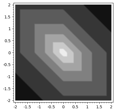
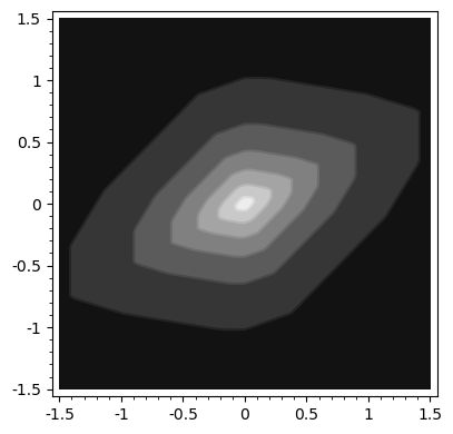
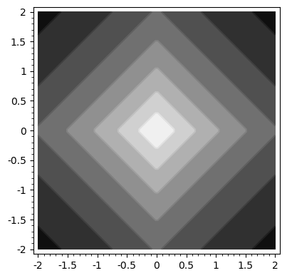
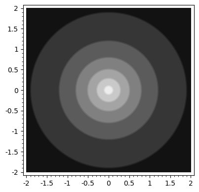
Figure 1. Contour plots of the kernels Ksubscript𝐾K_{\infty} under different intensity measures ΛΛ\Lambda. As the kernels are translation invariant, the plot shows the contour of the function xK(0,x)maps-to𝑥subscript𝐾0𝑥x\mapsto K_{\infty}(0,x) for d=2𝑑2d=2. From left to right: the Laplace kernel obtained from axis-aligned STIT; the exponential kernel obtained from the isotropic STIT; a kernel obtained from a STIT with three cut directions orthogonal to (1,0)10(1,0), (0,1)01(0,1) and (1,1)11(1,1); a kernel obtained from a STIT whose cut directions are ten random Gaussian vectors in dsuperscript𝑑\mathbb{R}^{d}. These plots show that the STIT can approximate many kernel functions.

Our second set of main results concerns density estimation and regression using STIT forests. The Mondrian density estimator was first introduced in [4]. It falls under the more general class of density estimation methods using random space partitions [47, 24, 22, 35]. In [27, 28] Mourtada, Gaï̈ffas, and Scornet gave minimax rates for the Mondrian regression estimator. Theorem 5.2 and Corollary 5.2 show that the STIT regression and density estimator are both consistent. For the Mondrian, Theorem 5.1 gives a precise understanding of the differences between the Mondrian forest, the Mondrian kernel, and the Laplace kernel method for density estimation. While the conceptual connection between forests and kernel estimates is well-known [7, 13, 23, 5, 6] and has been noted for the Mondrian case in regression [3], explicit formula like that of Theorem 5.1 have only been obtained for very few random forest models [2, 42], most notably the purely random forest [12]. Compared to purely random forests, Mondrian forests and more generally STIT forests are derived from a self-similar and stationary stochastic process. We crucially exploit these properties to overcome the main hurdle in the analysis of random forests in density estimation, namely, evaluating the volume of a cell in the partition. For the Mondrian case, our analysis uses the precise description of the distribution of a cell in the Mondrian process of Mourtada, Gaïffas, and Scornet [28]. This hints that their analysis can be generalized to obtain minimax rates for STIT regression and density estimators. We discuss this open problem, along with a number of other questions in Section 6. In summary, our paper points to more fruitful collaborations between stochastic geometry and machine learning.
Refer to caption
Refer to caption
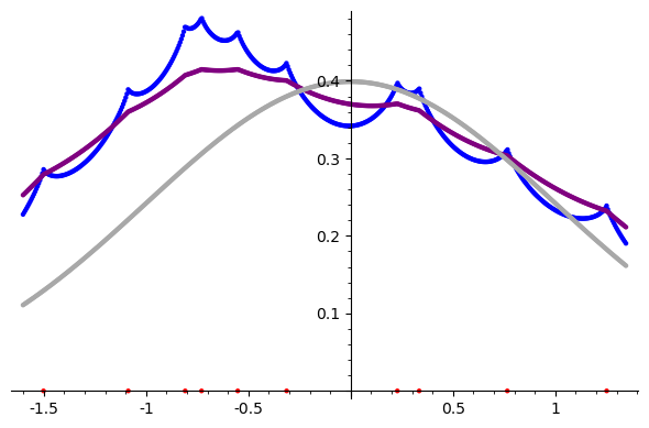
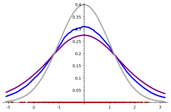
Figure 2. Density estimation with Laplace kernel (purple) and the Mondrian forest (blue). The points X1,,Xnsubscript𝑋1subscript𝑋𝑛X_{1},\dots,X_{n} (shown in red on the x𝑥x-axis) are sampled from the standard Gaussian (density shown in gray), with n=10𝑛10n=10 on the left figure, and n=1000𝑛1000n=1000 on the right. The Mondrian method gives more weight to existing data points, and less to those far away. For large number of points, empirically it gives faster convergence to the true density (gray).

2. Stochastic geometry background

The results we present here rely on the theory of stable under iteration (STIT) tessellations. We now summarize relevant results from the stochastic geometry literature that will be used throughout this paper. For a comprehensive text on stochastic geometry, we recommend [38].

2.1. Stable under iteration tessellations (STIT)

A tessellation of dsuperscript𝑑\mathbb{R}^{d} is a partition of the entire space into a locally finite collection of convex polytopes that have pairwise disjoint interior. One can think of a tessellation as either the collection of polytopes, called cells, or as the union of their boundaries. We will take the second view in this paper, in which a random tessellation can be considered as a random closed set, see [38]. For a random tessellation Y𝑌Y, we will denote the random collection of its cells by Cells(Y)Cells𝑌\mathrm{Cells}(Y). A random tessellation is stationary if its distribution is translation invariant, and isotropic if its distribution is invariant under rotations about the origin.

Stable under iteration (STIT) tessellations are a class of stationary random tessellations in dsuperscript𝑑\mathbb{R}^{d} introduced in [30]. A rich theory on their properties has since been developed, see [25, 29, 39, 41, 40]. We will now summarize the construction presented in [30]. Let dsuperscript𝑑\mathcal{H}^{d} denote the space of d1𝑑1d-1-dimensional affine hyperplanes in dsuperscript𝑑\mathbb{R}^{d} and let ΛΛ\Lambda be a locally finite and translation-invariant measure on dsuperscript𝑑\mathcal{H}^{d}. Assume there exist d𝑑d hyperplanes with linearly independent normal directions contained in the support of ΛΛ\Lambda. For Cd𝐶superscript𝑑C\subset\mathbb{R}^{d}, define the subset [C]ddelimited-[]𝐶superscript𝑑[C]\subseteq\mathcal{H}^{d} by

[C]:={Hd:HC}.assigndelimited-[]𝐶conditional-set𝐻superscript𝑑𝐻𝐶[C]:=\{H\in\mathcal{H}^{d}:H\cap C\neq\emptyset\}.

Assume ΛΛ\Lambda is normalized so that Λ([B(d,1)])=1Λdelimited-[]𝐵𝑑11\Lambda([B(d,1)])=1, where B(d,1)𝐵𝑑1B(d,1) is a ball in dsuperscript𝑑\mathbb{R}^{d} of unit diameter. Recall that a hyperplane in dsuperscript𝑑\mathbb{R}^{d} with normal vector ud𝑢superscript𝑑u\in\mathbb{R}^{d} and displacement t𝑡t\in\mathbb{R} is defined by Hd(u,t):={xd:x,u=t}assignsubscript𝐻𝑑𝑢𝑡conditional-set𝑥superscript𝑑𝑥𝑢𝑡H_{d}(u,t):=\{x\in\mathbb{R}^{d}:\langle x,u\rangle=t\}. The stationarity and normalization of the measure ΛΛ\Lambda imply that we can write

(1) Λ()=𝕊d11{Hd(u,t)}dtdϕ(u),Λsubscriptsuperscript𝕊𝑑1subscriptsubscript1subscript𝐻𝑑𝑢𝑡differential-d𝑡differential-ditalic-ϕ𝑢\displaystyle\Lambda(\cdot)=\int_{\mathbb{S}^{d-1}}\int_{\mathbb{R}}1_{\{H_{d}(u,t)\in\cdot\}}\mathrm{d}t\mathrm{d}\phi(u),

where ϕitalic-ϕ\phi is a probability measure on the unit sphere 𝕊d1superscript𝕊𝑑1\mathbb{S}^{d-1}, see Theorem 4.4.1 and (4.30) in [38].

To construct a STIT tessellation with intensity measure ΛΛ\Lambda, start from an initial bounded frame Wd𝑊superscript𝑑W\subset\mathbb{R}^{d}. Assign to W𝑊W a random exponential lifetime with parameter

Λ([W])Λdelimited-[]𝑊\displaystyle\Lambda([W]) =𝕊d11{Hd(u,t)W}dtdϕ(u)=𝕊d1(h(W,u)+h(W,u))dϕ(u),absentsubscriptsuperscript𝕊𝑑1subscriptsubscript1subscript𝐻𝑑𝑢𝑡𝑊differential-d𝑡differential-ditalic-ϕ𝑢subscriptsuperscript𝕊𝑑1𝑊𝑢𝑊𝑢differential-ditalic-ϕ𝑢\displaystyle=\int_{\mathbb{S}^{d-1}}\int_{\mathbb{R}}1_{\{H_{d}(u,t)\cap W\neq\emptyset\}}\mathrm{d}t\mathrm{d}\phi(u)=\int_{\mathbb{S}^{d-1}}\left(h(W,u)+h(W,-u)\right)\mathrm{d}\phi(u),

where h(W,u):=supxWu,xassign𝑊𝑢subscriptsupremum𝑥𝑊𝑢𝑥h(W,u):=\sup_{x\in W}\langle u,x\rangle is the support function for W𝑊W. When the lifetime expires, a random hyperplane is generated from the probability measure

Λ([W])Λ([W])=1Λ([W])𝕊d1h(W,u)h(W,u)1{Hd(u,t)}dtdϕ(u),\displaystyle\frac{\Lambda(\cdot\cap[W])}{\Lambda([W])}=\frac{1}{\Lambda([W])}\int_{\mathbb{S}^{d-1}}\int_{h(W,-u)}^{h(W,u)}1_{\{H_{d}(u,t)\in\cdot\}}\mathrm{d}t\mathrm{d}\phi(u),

splitting the window W𝑊W into two cells W1subscript𝑊1W_{1} and W2subscript𝑊2W_{2}. That is, the random hyperplane splitting W𝑊W has a random direction U𝑈U with distribution on 𝕊d1superscript𝕊𝑑1\mathbb{S}^{d-1} defined by

dΦ(u):=h(W,u)+h(W,u)Λ([W])dϕ(u),assigndΦ𝑢𝑊𝑢𝑊𝑢Λdelimited-[]𝑊ditalic-ϕ𝑢\mathrm{d}\Phi(u):=\frac{h(W,u)+h(W,-u)}{\Lambda([W])}\mathrm{d}\phi(u),

and conditioned on U𝑈U, the displacement is uniformly distributed in the interval from h(W,U)𝑊𝑈-h(W,-U) to h(W,U)𝑊𝑈h(W,U).

The construction continues recursively and independently in W1subscript𝑊1W_{1} and W2subscript𝑊2W_{2} until some fixed deterministic time λ>0𝜆0\lambda>0. We will denote the random tessellation constructed in W𝑊W up until time λ𝜆\lambda by YΛ(λ,W)subscript𝑌Λ𝜆𝑊Y_{\Lambda}(\lambda,W). The subscript ΛΛ\Lambda will be omitted when the intensity measure is clear from context. We denote by Y(λ)𝑌𝜆Y(\lambda) the tessellation on dsuperscript𝑑\mathbb{R}^{d} such that

(2) Y(λ)W=DY(λ,W),𝑌𝜆𝑊D𝑌𝜆𝑊\displaystyle Y(\lambda)\cap W\overset{\mathrm{D}}{=}Y(\lambda,W),

for all compact sets Wd𝑊superscript𝑑W\subset\mathbb{R}^{d}, the existence of which is stated in Theorem 1 of [31]. For all λ>0𝜆0\lambda>0, Y(λ)𝑌𝜆Y(\lambda) is stationary and satisfies the following scaling property:

λY(λ)=DY(1).𝜆𝑌𝜆D𝑌1\lambda Y(\lambda)\overset{\mathrm{D}}{=}Y(1).

In addition, there is a closed formula for the capacity functional of Y(λ)𝑌𝜆Y(\lambda). Letting 𝒞𝒞\mathcal{C} denote the set of compact subsets of dsuperscript𝑑\mathbb{R}^{d}, the capacity functional of a random closed set Z𝑍Z is defined by

TZ(C):=(ZC),C𝒞.formulae-sequenceassignsubscript𝑇𝑍𝐶𝑍𝐶𝐶𝒞T_{Z}(C):=\mathbb{P}(Z\cap C\neq\emptyset),\qquad C\in\mathcal{C}.

In particular, for C𝒞𝐶𝒞C\in\mathcal{C} with one connected component, it was shown in [31] that for a STIT tessellation with intensity measure ΛΛ\Lambda,

(3) TY(λ)(C)=1eλΛ([C]).subscript𝑇𝑌𝜆𝐶1superscript𝑒𝜆Λdelimited-[]𝐶\displaystyle T_{Y(\lambda)}(C)=1-e^{-\lambda\Lambda([C])}.

When ϕitalic-ϕ\phi is the uniform distribution over the basis vectors {ei}i=1dsuperscriptsubscriptsubscript𝑒𝑖𝑖1𝑑\{e_{i}\}_{i=1}^{d}, that is, when

(4) Λ()=1di=1d1{Hd(ei,t)}dt,Λ1𝑑superscriptsubscript𝑖1𝑑subscriptsubscript1subscript𝐻𝑑subscript𝑒𝑖𝑡differential-d𝑡\displaystyle\Lambda(\cdot)=\frac{1}{d}\sum_{i=1}^{d}\int_{\mathbb{R}}1_{\{H_{d}(e_{i},t)\in\cdot\}}\mathrm{d}t,

the STIT tessellation construction corresponds to a Mondrian process. Another particular case is when ϕ=σitalic-ϕ𝜎\phi=\sigma, where σ𝜎\sigma denotes the normalized spherical Lebesgue measure on 𝕊d1superscript𝕊𝑑1\mathbb{S}^{d-1}. This intensity measure ΛΛ\Lambda and the resulting tessellation are isotropic as well as stationary. This case is studied in [11], where they refer to it as the uRTP, or the uniform random tessellation process.

Example 2.1.

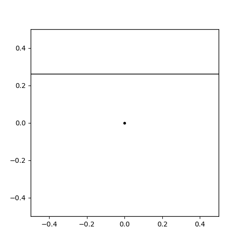
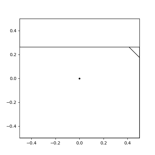
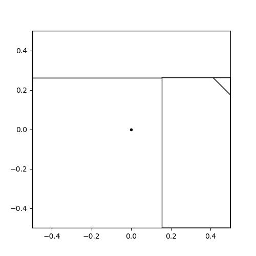
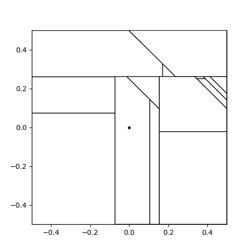
Let W=[0.5,0.5]2𝑊superscript0.50.52W=[-0.5,0.5]^{2} and let dϕ(u)=i=13δuiditalic-ϕ𝑢superscriptsubscript𝑖13subscript𝛿subscript𝑢𝑖\mathrm{d}\phi(u)=\sum_{i=1}^{3}\delta_{u_{i}}, where u1=(1,0)subscript𝑢110u_{1}=(1,0), u2=(0,1)subscript𝑢201u_{2}=(0,1), and u3=(1/2,1/2)subscript𝑢31212u_{3}=(1/\sqrt{2},1/\sqrt{2}). When the exponential lifetime with parameter Λ([W])Λdelimited-[]𝑊\Lambda([W]) expires, a cut is made as follows. The direction is uisubscript𝑢𝑖u_{i} with probability {12+2,i=1,222+2,i=3.cases122𝑖12222𝑖3\begin{cases}\frac{1}{2+\sqrt{2}},&i=1,2\\ \frac{\sqrt{2}}{2+\sqrt{2}},&i=3.\end{cases} Then the displacement t𝑡t is uniform on [0.5,0.5]0.50.5[-0.5,0.5] if the direction is u1subscript𝑢1u_{1} or u2subscript𝑢2u_{2} and is uniform on [12,12]1212[-\frac{1}{\sqrt{2}},\frac{1}{\sqrt{2}}] if the direction is u3subscript𝑢3u_{3}. Figure 3 shows a simulation of this STIT up to lifetime 999.

Refer to caption
Refer to caption
Refer to caption
Refer to caption
Figure 3. An example STIT process with three directions. Each cell W𝑊W has an independent exponential clock with mean Λ([W])Λdelimited-[]𝑊\Lambda([W]). When the clock rings, the cell is cut by a hyperplane drawn from the specified distribution ΛΛ\Lambda conditioned to hit this cell. In this simulation, at time t=0𝑡0t=0 we start with the unit square W=[0.5,0.5]2𝑊superscript0.50.52W=[-0.5,0.5]^{2}, and ran until time t=9𝑡9t=9, called the lifetime of the STIT. The first three figures show the first three cuts, while the last figure shows the STIT at time t=9𝑡9t=9, which has 14 cuts.

2.2. The typical cell of a STIT tessellation

Let Y(λ)𝑌𝜆Y(\lambda) denote the stationary STIT tessellation on dsuperscript𝑑\mathbb{R}^{d} with intensity measure ΛΛ\Lambda and lifetime parameter λ𝜆\lambda. Let c(C)𝑐𝐶c(C) be the center of the inball of a convex body Cd𝐶superscript𝑑C\subset\mathbb{R}^{d}, and let 𝒞0:={Cd:C is a non-empty convex body with c(C)=0}assignsubscript𝒞0conditional-set𝐶superscript𝑑𝐶 is a non-empty convex body with 𝑐𝐶0\mathcal{C}_{0}:=\{C\subset\mathbb{R}^{d}:C\text{ is a non-empty convex body with }c(C)=0\}. Let V(C)𝑉𝐶V(C) denote the d𝑑d-dimensional volume of C𝐶C. The typical cell of Y(λ)𝑌𝜆Y(\lambda) is the random closed set Z𝑍Z with probability distribution on 𝒞0subscript𝒞0\mathcal{C}_{0} given by the following limit (see [38, (4.8) and (4.9)]): for any convex body Wd𝑊superscript𝑑W\subset\mathbb{R}^{d} with V(W)>0𝑉𝑊0V(W)>0,

(A):=limr1V(rW)𝔼CCells(Y(λ)),CrW1A(Cc(C)).assign𝐴subscript𝑟1𝑉𝑟𝑊𝔼subscriptformulae-sequence𝐶Cells𝑌𝜆𝐶𝑟𝑊subscript1𝐴𝐶𝑐𝐶\mathbb{Q}(A):=\lim_{r\to\infty}\frac{1}{V(rW)}\mathbb{E}\sum_{C\in\mathrm{Cells}(Y(\lambda)),C\cap rW\neq\emptyset}1_{A}(C-c(C)).

By Theorem 1 in [40], Z𝑍Z has the same distribution as the typical cell of a Poisson hyperplane tessellation with mean measure λΛ𝜆Λ\lambda\Lambda. By Campbell’s theorem (Theorem 3.1.2 in [38]) and [38, (4.3)], for any nonnegative measurable function f𝑓f on the space of convex bodies in dsuperscript𝑑\mathbb{R}^{d},

(5) 𝔼[CCells(Y(λ))f(C)]=1𝔼[V(Z)]𝔼[df(Z+y)dy].𝔼delimited-[]subscript𝐶Cells𝑌𝜆𝑓𝐶1𝔼delimited-[]𝑉𝑍𝔼delimited-[]subscriptsuperscript𝑑𝑓𝑍𝑦differential-d𝑦\displaystyle\mathbb{E}\left[\sum_{C\in\mathrm{Cells}(Y(\lambda))}f(C)\right]=\frac{1}{\mathbb{E}[V(Z)]}\mathbb{E}\left[\int_{\mathbb{R}^{d}}f(Z+y)\mathrm{d}y\right].

2.3. Associated Zonoid

A non-empty convex body ΠΠ\Pi is called a centered zonoid if its support function takes the form h(Π,v)=𝕊d1|u,v|dψ(u)Π𝑣subscriptsuperscript𝕊𝑑1𝑢𝑣differential-d𝜓𝑢h(\Pi,v)=\int_{\mathbb{S}^{d-1}}|\langle u,v\rangle|\mathrm{d}\psi(u) for some even and finite measure ψ𝜓\psi on the unit sphere [38, p.614]. For a stationary measure ΛΛ\Lambda on dsuperscript𝑑\mathcal{H}^{d} as in (1) and constant λ>0𝜆0\lambda>0, define the zonoid ΠΠ\Pi with support function

(6) h(Π,v)=λ2Λ([[0,v]])=λ2𝕊d1|u,v|dϕ(u).Π𝑣𝜆2Λdelimited-[]0𝑣𝜆2subscriptsuperscript𝕊𝑑1𝑢𝑣differential-ditalic-ϕ𝑢\displaystyle h(\Pi,v)=\frac{\lambda}{2}\Lambda([[0,v]])=\frac{\lambda}{2}\int_{\mathbb{S}^{d-1}}|\langle u,v\rangle|\mathrm{d}\phi(u).

ΠΠ\Pi is called the associated zonoid of the measure λΛ𝜆Λ\lambda\Lambda, or of the stationary STIT with intensity measure ΛΛ\Lambda and lifetime parameter λ𝜆\lambda. For each zonoid ΠΠ\Pi, there is a unique stationary measure and intensity, and thus a unique STIT tessellation, for which ΠΠ\Pi is the associated zonoid, see [38, p.156].

3. General cut directions as projections of axis-aligned

Consider a stationary STIT tessellation Y𝑌Y in dsuperscript𝑑\mathbb{R}^{d} where the directional distribution of the hyperplanes is the uniform distribution over nd𝑛𝑑n\geq d fixed directions u1,,un𝕊d1subscript𝑢1subscript𝑢𝑛superscript𝕊𝑑1u_{1},\ldots,u_{n}\in\mathbb{S}^{d-1}. While it is known that the intersection of a STIT tessellation with a lower dimensional linear subspace is distributed as a STIT tessellation [41, 31], to the best of our knowledge, Theorem 3.1 below is the first to give an explicit formula that shows any STIT with finitely many cut directions can be obtained from the intersection of an axis-aligned STIT in a higher dimension with an appropriate subspace.

Theorem 3.1.

Let u1,,unsubscript𝑢1subscript𝑢𝑛u_{1},\ldots,u_{n} be n𝑛n points on the unit sphere 𝕊d1superscript𝕊𝑑1\mathbb{S}^{d-1}, and define U:dn:𝑈superscript𝑑superscript𝑛U:\mathbb{R}^{d}\to\mathbb{R}^{n} to be a n×d𝑛𝑑n\times d matrix with rows u1,,unsubscript𝑢1subscript𝑢𝑛u_{1},\ldots,u_{n}. Let Y𝑌Y be a STIT tessellation in dsuperscript𝑑\mathbb{R}^{d} with associated intensity measure

(7) ΛU()=1ni=1n1{Hd(ui,t)}dt,subscriptΛ𝑈1𝑛superscriptsubscript𝑖1𝑛subscriptsubscript1subscript𝐻𝑑subscript𝑢𝑖𝑡differential-d𝑡\displaystyle\Lambda_{U}(\cdot)=\frac{1}{n}\sum_{i=1}^{n}\int_{\mathbb{R}}1_{\{H_{d}(u_{i},t)\in\cdot\}}\mathrm{d}t,

where Hd(u,t):={xd:x,u=t}assignsubscript𝐻𝑑𝑢𝑡conditional-set𝑥superscript𝑑𝑥𝑢𝑡H_{d}(u,t):=\{x\in\mathbb{R}^{d}:\langle x,u\rangle=t\}. Let L𝐿L be the linear subspace of nsuperscript𝑛\mathbb{R}^{n} spanned by the columns of U𝑈U. Then, U(Y)𝑈𝑌U(Y) has the same distribution as the intersection of a Mondrian process in nsuperscript𝑛\mathbb{R}^{n} with the subspace L𝐿L.

For the STIT tessellation with intensity measure ΛUsubscriptΛ𝑈\Lambda_{U}, a cell is split by a hyperplane supported by uisubscript𝑢𝑖u_{i} with probability proportional to the length of its projection onto the line spanned by uisubscript𝑢𝑖u_{i}. When the uisubscript𝑢𝑖u_{i}’s are the d𝑑d standard coordinate vectors, then one obtains an axis-aligned STIT, i.e., the Mondrian process. Theorem 3.1 states that using finitely many cut directions has the same effect as performing a linear embedding of the data in higher dimensions and then partitioning it with the Mondrian process.

Proof of Theorem 3.1.

In [31], Lemma 4 and Corollary 1 show that the capacity functional for a STIT tessellation is determined by its associated intensity measure on the space of hyperplanes. Thus it suffices to show that for any Borel set Cd𝐶superscript𝑑C\subset\mathbb{R}^{d},

ΛU([C])=ΛM([U(C)]),subscriptΛ𝑈delimited-[]𝐶subscriptΛ𝑀delimited-[]𝑈𝐶\Lambda_{U}([C])=\Lambda_{M}([U(C)]),

where ΛMsubscriptΛ𝑀\Lambda_{M} is the measure on dsuperscript𝑑\mathcal{H}^{d} associated to the Mondrian process as in (4).

Letting {ei(n)}i=1nsuperscriptsubscriptsubscriptsuperscript𝑒𝑛𝑖𝑖1𝑛\{e^{(n)}_{i}\}_{i=1}^{n} denote the standard basis in nsuperscript𝑛\mathbb{R}^{n}, we see that for any xHd(ui,t)𝑥subscript𝐻𝑑subscript𝑢𝑖𝑡x\in H_{d}(u_{i},t),

Ux,ei(n)=x,UTei(n)=x,ui=t.𝑈𝑥subscriptsuperscript𝑒𝑛𝑖𝑥superscript𝑈𝑇superscriptsubscript𝑒𝑖𝑛𝑥subscript𝑢𝑖𝑡\langle Ux,e^{(n)}_{i}\rangle=\langle x,U^{T}e_{i}^{(n)}\rangle=\langle x,u_{i}\rangle=t.

Thus, U(Hd(ui,t))=Hn(ei(n),t)L𝑈subscript𝐻𝑑subscript𝑢𝑖𝑡subscript𝐻𝑛subscriptsuperscript𝑒𝑛𝑖𝑡𝐿U(H_{d}(u_{i},t))=H_{n}(e^{(n)}_{i},t)\cap L. Then, for any Borel set Cd𝐶superscript𝑑C\subset\mathbb{R}^{d},

ΛU([C])subscriptΛ𝑈delimited-[]𝐶\displaystyle\Lambda_{U}([C]) =1ni=1n1{Hd(ui,t)C}dt=1ni=1n1{U(Hd(ui,t))U(C)}dtabsent1𝑛superscriptsubscript𝑖1𝑛subscriptsubscript1subscript𝐻𝑑subscript𝑢𝑖𝑡𝐶differential-d𝑡1𝑛superscriptsubscript𝑖1𝑛subscriptsubscript1𝑈subscript𝐻𝑑subscript𝑢𝑖𝑡𝑈𝐶differential-d𝑡\displaystyle=\frac{1}{n}\sum_{i=1}^{n}\int_{\mathbb{R}}1_{\{H_{d}(u_{i},t)\cap C\neq\emptyset\}}\mathrm{d}t=\frac{1}{n}\sum_{i=1}^{n}\int_{\mathbb{R}}1_{\{U(H_{d}(u_{i},t))\cap U(C)\neq\emptyset\}}\mathrm{d}t
=1ni=1n1{(Hn(ei(n),t)L)U(C)}dtabsent1𝑛superscriptsubscript𝑖1𝑛subscriptsubscript1subscript𝐻𝑛subscriptsuperscript𝑒𝑛𝑖𝑡𝐿𝑈𝐶differential-d𝑡\displaystyle=\frac{1}{n}\sum_{i=1}^{n}\int_{\mathbb{R}}1_{\{(H_{n}(e^{(n)}_{i},t)\cap L)\cap U(C)\neq\emptyset\}}\mathrm{d}t
=1ni=1n1{Hn(ei(n),t)U(C)}dt=ΛM([U(C)]).absent1𝑛superscriptsubscript𝑖1𝑛subscriptsubscript1subscript𝐻𝑛subscriptsuperscript𝑒𝑛𝑖𝑡𝑈𝐶differential-d𝑡subscriptΛ𝑀delimited-[]𝑈𝐶\displaystyle=\frac{1}{n}\sum_{i=1}^{n}\int_{\mathbb{R}}1_{\{H_{n}(e^{(n)}_{i},t)\cap U(C)\neq\emptyset\}}\mathrm{d}t=\Lambda_{M}([U(C)]).

This completes the proof. ∎

4. STIT Kernel Approximation

When one uses the Mondrian process to randomly approximate kernels, there is much to gain from considering more general cuts. While the standard Mondrian approximates the Laplace kernel [3, Proposition 1], we show that one can approximate many other kernels with the general STIT. In particular, the exponential kernel k(x,y)=exp(xy2/σ)𝑘𝑥𝑦subscriptnorm𝑥𝑦2𝜎k(x,y)=\exp(-\|x-y\|_{2}/\sigma) can be approximated by the uniform STIT, whose cut directions are chosen uniformly at random from the sphere in dsuperscript𝑑\mathbb{R}^{d}.

4.1. Characterization of limiting STIT kernels

Following [3], we define a random feature map corresponding to a STIT tessellation Y(λ)𝑌𝜆Y(\lambda) as follows. First, define a feature map ϕitalic-ϕ\phi that maps a location xd𝑥superscript𝑑x\in\mathbb{R}^{d} to a column vector with a single non-zero entry that indicates the cell of the partition that x𝑥x lies in. We can then define the kernel

K1(x,y):=ϕ(x)Tϕ(y)={1,x,y in same cell of Y(λ)0,otherwise.assignsubscript𝐾1𝑥𝑦italic-ϕsuperscript𝑥𝑇italic-ϕ𝑦cases1𝑥𝑦 in same cell of 𝑌𝜆0otherwiseK_{1}(x,y):=\phi(x)^{T}\phi(y)=\begin{cases}1,&x,y\text{ in same cell of }Y(\lambda)\\ 0,&\text{otherwise}.\end{cases}

Then, let Y1,,YMsubscript𝑌1subscript𝑌𝑀Y_{1},\ldots,Y_{M} be M𝑀M i.i.d. copies of Y(λ)𝑌𝜆Y(\lambda). Concatenating the M𝑀M i.i.d. corresponding random feature maps ϕ(1),,ϕ(M)superscriptitalic-ϕ1superscriptitalic-ϕ𝑀\phi^{(1)},\ldots,\phi^{(M)} into a single random feature map and scaling, we define the STIT kernel of order M𝑀M:

KM(x,y):=1Mm=1Mϕ(m)(x)Tϕ(m)(y)=1Mm=1M1{y,x in same cell of Ym}.assignsubscript𝐾𝑀𝑥𝑦1𝑀superscriptsubscript𝑚1𝑀superscriptitalic-ϕ𝑚superscript𝑥𝑇superscriptitalic-ϕ𝑚𝑦1𝑀superscriptsubscript𝑚1𝑀subscript1𝑦𝑥 in same cell of subscript𝑌𝑚K_{M}(x,y):=\frac{1}{M}\sum_{m=1}^{M}\phi^{(m)}(x)^{T}\phi^{(m)}(y)=\frac{1}{M}\sum_{m=1}^{M}1_{\{y,x\text{ in same cell of }Y_{m}\}}.
Theorem 4.1.

Consider a stationary STIT tessellation Y(λ)𝑌𝜆Y(\lambda) in dsuperscript𝑑\mathbb{R}^{d} with associated intensity measure ΛΛ\Lambda and lifetime parameter λ𝜆\lambda. For each M𝑀M, define KMsubscript𝐾𝑀K_{M}, the STIT kernel of order M𝑀M, as above. Then,

(8) limMKM(x,y)=K(x,y):=eλΛ([[x,y]]),a.s.,formulae-sequencesubscript𝑀subscript𝐾𝑀𝑥𝑦subscript𝐾𝑥𝑦assignsuperscript𝑒𝜆Λdelimited-[]𝑥𝑦𝑎𝑠\displaystyle\lim_{M\to\infty}K_{M}(x,y)=K_{\infty}(x,y):=e^{-\lambda\Lambda([[x,y]])},\qquad a.s.,

where [[x,y]]delimited-[]𝑥𝑦[[x,y]] denotes the set of hyperplanes hitting the line segment connecting x𝑥x and y𝑦y in dsuperscript𝑑\mathbb{R}^{d}.

Proof of Theorem 4.1.

Let Y1,,YMsubscript𝑌1subscript𝑌𝑀Y_{1},\ldots,Y_{M} be i.i.d. realizations of a STIT tessellation Y(λ)𝑌𝜆Y(\lambda) with stationary intensity measure ΛΛ\Lambda. As noted in [3], the strong law of large numbers gives the following limit:

limMKM(x,y)subscript𝑀subscript𝐾𝑀𝑥𝑦\displaystyle\lim_{M\to\infty}K_{M}(x,y) =limM1Mm=1M1{x,y in same cell of Ym}absentsubscript𝑀1𝑀superscriptsubscript𝑚1𝑀subscript1𝑥𝑦 in same cell of subscript𝑌𝑚\displaystyle=\lim_{M\to\infty}\frac{1}{M}\sum_{m=1}^{M}1_{\{x,y\text{ in same cell of }Y_{m}\}}
=(x,y in same cell of Y(λ)),a.s.formulae-sequenceabsent𝑥𝑦 in same cell of 𝑌𝜆as\displaystyle=\mathbb{P}(x,y\text{ in same cell of }Y(\lambda)),\qquad\mathrm{a.s.}

We shall derive this probability from the capacity functional formula (3). For x,yd𝑥𝑦superscript𝑑x,y\in\mathbb{R}^{d}, (3) immediately gives

(x,y in same cell of Y(λ))=(Y(λ)[x,y]=)=exp(λΛ([[x,y]])).𝑥𝑦 in same cell of 𝑌𝜆𝑌𝜆𝑥𝑦𝜆Λdelimited-[]𝑥𝑦\displaystyle\mathbb{P}(x,y\text{ in same cell of }Y(\lambda))=\mathbb{P}(Y(\lambda)\cap[x,y]=\emptyset)=\exp\left(-\lambda\Lambda([[x,y]])\right).

We now give some examples. If Λ()Λ\Lambda(\cdot) is isotropic, then

(9) K(x,y)=e2λκd1dκdxy2,subscript𝐾𝑥𝑦superscript𝑒2𝜆subscript𝜅𝑑1𝑑subscript𝜅𝑑subscriptnorm𝑥𝑦2\displaystyle K_{\infty}(x,y)=e^{-\frac{2\lambda\kappa_{d-1}}{d\kappa_{d}}\|x-y\|_{2}},

where κdsubscript𝜅𝑑\kappa_{d} is the volume of the d𝑑d-dimensional unit ball. If Λ()Λ\Lambda(\cdot) is defined by (7), then

(10) K(x,y)=eλnU(xy)1,subscript𝐾𝑥𝑦superscript𝑒𝜆𝑛subscriptnorm𝑈𝑥𝑦1\displaystyle K_{\infty}(x,y)=e^{-\frac{\lambda}{n}\|U(x-y)\|_{1}},

where U𝑈U is the n×d𝑛𝑑n\times d matrix with rows u1,,unsubscript𝑢1subscript𝑢𝑛u_{1},\ldots,u_{n}.

To show (9) and (10), note that the hyperplane H(ui,t)𝐻subscript𝑢𝑖𝑡H(u_{i},t) hits the line segment [x,y]𝑥𝑦[x,y] if and only if ui,xtui,ysubscript𝑢𝑖𝑥𝑡subscript𝑢𝑖𝑦\langle u_{i},x\rangle\leq t\leq\langle u_{i},y\rangle when ui,yx0subscript𝑢𝑖𝑦𝑥0\langle u_{i},y-x\rangle\geq 0 or ui,ytui,xsubscript𝑢𝑖𝑦𝑡subscript𝑢𝑖𝑥\langle u_{i},y\rangle\leq t\leq\langle u_{i},x\rangle when ui,yx<0subscript𝑢𝑖𝑦𝑥0\langle u_{i},y-x\rangle<0. Thus, in the isotopic case,

Λ([[x,y]])Λdelimited-[]𝑥𝑦\displaystyle\Lambda([[x,y]]) =𝕊d11{H(u,t)[x,y]}dtdσ(u)=𝕊d101{t|xy,u|}𝑑tσ(du)absentsubscriptsuperscript𝕊𝑑1subscriptsubscript1𝐻𝑢𝑡𝑥𝑦differential-d𝑡differential-d𝜎𝑢subscriptsuperscript𝕊𝑑1superscriptsubscript0subscript1𝑡𝑥𝑦𝑢differential-d𝑡𝜎𝑑𝑢\displaystyle=\int_{\mathbb{S}^{d-1}}\int_{\mathbb{R}}1_{\{H(u,t)\cap[x,y]\neq\emptyset\}}\mathrm{d}t\mathrm{d}\sigma(u)=\int_{\mathbb{S}^{d-1}}\int_{0}^{\infty}1_{\{t\leq|\langle x-y,u\rangle|\}}dt\sigma(du)
=𝕊d1|xy,u|σ(du)=2κd1dκdxy2,absentsubscriptsuperscript𝕊𝑑1𝑥𝑦𝑢𝜎𝑑𝑢2subscript𝜅𝑑1𝑑subscript𝜅𝑑subscriptnorm𝑥𝑦2\displaystyle=\int_{\mathbb{S}^{d-1}}|\langle x-y,u\rangle|\sigma(du)=\frac{2\kappa_{d-1}}{d\kappa_{d}}\|x-y\|_{2},

and for ΛΛ\Lambda as in (7),

Λ([[x,y]])Λdelimited-[]𝑥𝑦\displaystyle\Lambda([[x,y]]) =1ni=1n1{H(ui,t)[x,y]}dt=1ni=1n01{t|ui,xy|}dtabsent1𝑛superscriptsubscript𝑖1𝑛subscriptsubscript1𝐻subscript𝑢𝑖𝑡𝑥𝑦differential-d𝑡1𝑛superscriptsubscript𝑖1𝑛superscriptsubscript0subscript1𝑡subscript𝑢𝑖𝑥𝑦differential-d𝑡\displaystyle=\frac{1}{n}\sum_{i=1}^{n}\int_{\mathbb{R}}1_{\{H(u_{i},t)\cap[x,y]\neq\emptyset\}}\mathrm{d}t=\frac{1}{n}\sum_{i=1}^{n}\int_{0}^{\infty}1_{\{t\leq|\langle u_{i},x-y\rangle|\}}\mathrm{d}t
=1ni=1n|ui,xy|=1nU(xy)1,absent1𝑛superscriptsubscript𝑖1𝑛subscript𝑢𝑖𝑥𝑦1𝑛subscriptnorm𝑈𝑥𝑦1\displaystyle=\frac{1}{n}\sum_{i=1}^{n}|\langle u_{i},x-y\rangle|=\frac{1}{n}\|U(x-y)\|_{1},

where Un×d𝑈superscript𝑛𝑑U\in\mathbb{R}^{n\times d} is the matrix with rows u1,,unsubscript𝑢1subscript𝑢𝑛u_{1},\ldots,u_{n}.

The following corollary characterizes all stationary kernels that can be approximated as in Theorem 4.1 in terms of the associated zonoid of the STIT tessellation (see section 2.3). In particular, not all positive definite kernels can be approximated this way. The corollary follows directly from (8) and (6), as well as Theorem 4.2 in [26], which states that a random vector η𝜂\eta has a symmetric α𝛼\alpha-stable distribution with α=1𝛼1\alpha=1 if and only if there is a unique centered zonoid ΠΠ\Pi such that the characteristic function of η𝜂\eta takes the form Φη(v)=eh(Π,v)subscriptΦ𝜂𝑣superscript𝑒Π𝑣\Phi_{\eta}(v)=e^{-h(\Pi,v)}, vd𝑣superscript𝑑v\in\mathbb{R}^{d}.

Corollary 4.1.

Let K(x,y)=K0(xy)𝐾𝑥𝑦subscript𝐾0𝑥𝑦K(x,y)=K_{0}(x-y) be a stationary positive definite kernel. There exists a stationary STIT tessellation Y𝑌Y in dsuperscript𝑑\mathbb{R}^{d} with intensity measure ΛΛ\Lambda and lifetime parameter λ𝜆\lambda such that (8) holds for this kernel if and only if there exists a centered zonoid ΠdΠsuperscript𝑑\Pi\subset\mathbb{R}^{d} such that

K0(v)=eλΛ([[0,v]])=e2h(Π,v),vd.formulae-sequencesubscript𝐾0𝑣superscript𝑒𝜆Λdelimited-[]0𝑣superscript𝑒2Π𝑣𝑣superscript𝑑K_{0}(v)=e^{-\lambda\Lambda([[0,v]])}=e^{-2h(\Pi,v)},\,v\in\mathbb{R}^{d}.

In particular, this holds if and only if K0(v)subscript𝐾0𝑣K_{0}(v) is the characteristic function of a multivariate Cauchy distribution.

A larger class of kernels can be approximated by adding additional randomness to the STIT process. The next result characterizes all kernels that can be approximated by random features obtained from STIT tessellations with a random lifetime parameter.

Theorem 4.2.

Let ξ𝜉\xi be a non-negative real-valued random variable. Let Y𝑌Y be a random tessellation such that conditioned on ξ𝜉\xi, Y𝑌Y is a stationary STIT tessellation with intensity measure ΛΛ\Lambda and lifetime parameter ξ𝜉\xi. The limiting kernel Ksubscript𝐾K_{\infty} based on i.i.d. copies of Y𝑌Y as in Theorem 4.1 is of the form

K(x,y)=Φ(h(Π,xy)),subscript𝐾𝑥𝑦ΦΠ𝑥𝑦K_{\infty}(x,y)=\Phi(h(\Pi,x-y)),

where ΠΠ\Pi is centered zonoid with support function h(Π,v)=𝕊d1|u,v|dϕ(u)Π𝑣subscriptsuperscript𝕊𝑑1𝑢𝑣differential-ditalic-ϕ𝑢h(\Pi,v)=\int_{\mathbb{S}^{d-1}}|\langle u,v\rangle|\mathrm{d}\phi(u), and ΦΦ\Phi is the Laplace transform of ξ𝜉\xi.

Proof.

Let ξ𝜉\xi be a non-negative real-valued random variable and ΛΛ\Lambda a stationary measure on the space of hyperplanes with associated zonoid ΠΠ\Pi. Define the random kernel KMsubscript𝐾𝑀K_{M} and its limit Ksubscript𝐾K_{\infty} as in Theorem 4.1 with respect to the random tessellation generated by first sampling from ξ𝜉\xi and then sampling a STIT process with intensity measure ΛΛ\Lambda and lifetime parameter ξ𝜉\xi. Conditioning on ξ𝜉\xi gives

K(v)=𝔼[𝔼[K(v)|ξ]]=𝔼[eξΛ([[0,v]])]=𝔼[eξ𝕊d1|u,v|dϕ(u)]=𝔼[eξh(Π,v)].subscript𝐾𝑣𝔼delimited-[]𝔼delimited-[]conditionalsubscript𝐾𝑣𝜉𝔼delimited-[]superscript𝑒𝜉Λdelimited-[]0𝑣𝔼delimited-[]superscript𝑒𝜉subscriptsuperscript𝕊𝑑1𝑢𝑣differential-ditalic-ϕ𝑢𝔼delimited-[]superscript𝑒𝜉Π𝑣K_{\infty}(v)=\mathbb{E}[\mathbb{E}[K_{\infty}(v)|\xi]]=\mathbb{E}\left[e^{-\xi\Lambda([[0,v]])}\right]=\mathbb{E}\left[e^{-\xi\int_{\mathbb{S}^{d-1}}|\langle u,v\rangle|\mathrm{d}\phi(u)}\right]=\mathbb{E}\left[e^{-\xi h(\Pi,v)}\right].

This is the Laplace transform of the random variable ξ𝜉\xi at the value h(Π,v)Π𝑣h(\Pi,v). ∎

For the following corollary, recall that a function Φ:[0,):Φ0\Phi:[0,\infty)\to\mathbb{R} is completely monotone if ΦΦ\Phi is continuous on [0,)0[0,\infty), smooth on (0,)0(0,\infty), and

(1)kΦ(k)(r)0,r>0,k=0,1,2,,formulae-sequencesuperscript1𝑘superscriptΦ𝑘𝑟0formulae-sequence𝑟0𝑘012(-1)^{k}\Phi^{(k)}(r)\geq 0,\quad r>0,k=0,1,2,\ldots,

where Φ(k)superscriptΦ𝑘\Phi^{(k)} is the k𝑘k-th order derivative of ΦΦ\Phi.

Corollary 4.2.

Define Y𝑌Y as in Theorem 4.1. Let K𝐾K be a positive definite stationary kernel of the form

K(x,y)=Φ(h(Π,xy))𝐾𝑥𝑦ΦΠ𝑥𝑦K(x,y)=\Phi(h(\Pi,x-y))

for some centered zonoid ΠΠ\Pi and function Φ:+:Φsubscript\Phi:\mathbb{R}_{+}\to\mathbb{R}. K𝐾K can be approximated as in (8) with i.i.d. copies of Y𝑌Y for some distribution of ξ𝜉\xi if and only if ΦΦ\Phi is completely monotone.

Proof.

The Hausdorff-Bernstein-Widder Theorem says that ϕitalic-ϕ\phi is completely monotone if and only if ϕitalic-ϕ\phi the Laplace transform of a finite non-negative Borel measure μ𝜇\mu on [0,)0[0,\infty). Thus, a stationary kernel K𝐾K can be approximated with the tessellation Y𝑌Y for some ξ𝜉\xi if and only if K(x,y)=ϕ(h(Π,xy))𝐾𝑥𝑦italic-ϕΠ𝑥𝑦K(x,y)=\phi(h(\Pi,x-y)) for a completely monotone function ϕitalic-ϕ\phi.

Some examples of completely monotone functions ΦΦ\Phi and the corresponding random lifetime parameter ξ𝜉\xi needed to approximate a kernel of the form Φ(h(Π,))ΦΠ\Phi(h(\Pi,\cdot)) include the following:

  1. (1)

    If ξ𝜉\xi is a gamma random variable ξ𝜉\xi with shape parameter α𝛼\alpha and rate parameter λ𝜆\lambda, then

    K(x,y)=(λλ+h(Π,v))α.subscript𝐾𝑥𝑦superscript𝜆𝜆Π𝑣𝛼K_{\infty}(x,y)=\left(\frac{\lambda}{\lambda+h(\Pi,v)}\right)^{\alpha}.
  2. (2)

    If ξ𝜉\xi is uniformly distributed on the interval [a,b]𝑎𝑏[a,b] for 0<a<b<0𝑎𝑏0<a<b<\infty, then

    K(x,y)=eh(Π,v)aeh(Π,v)bh(Π,v)(ba),subscript𝐾𝑥𝑦superscript𝑒Π𝑣𝑎superscript𝑒Π𝑣𝑏Π𝑣𝑏𝑎K_{\infty}(x,y)=\frac{e^{-h(\Pi,v)a}-e^{-h(\Pi,v)b}}{h(\Pi,v)(b-a)},

4.2. Convergence rates of STIT kernels

We next turn to the rate at which the STIT kernel converges over any bounded window W𝑊W. First, consider the case that KMsubscript𝐾𝑀K_{M} is generated by M𝑀M i.i.d. copies of a STIT tessellation Y(λ)𝑌𝜆Y(\lambda) with lifetime parameter λ𝜆\lambda and intensity measure ΛUsubscriptΛ𝑈\Lambda_{U} as in (7). Proposition 2 in [3] states that for the Mondrian kernel K~Msubscript~𝐾𝑀\tilde{K}_{M} on nsuperscript𝑛\mathbb{R}^{n} with uniform measure ΛΛ\Lambda in all axis-aligned directions and lifetime λn𝜆𝑛\lambda n,

(11) (supx,yW|K~M(x,y)K~(x,y)|δ)subscriptsupremum𝑥𝑦𝑊subscript~𝐾𝑀𝑥𝑦subscript~𝐾𝑥𝑦𝛿\displaystyle\mathbb{P}\left(\sup_{x,y\in W}|\tilde{K}_{M}(x,y)-\tilde{K}_{\infty}(x,y)|\geq\delta\right)
(21/(2n)4M2λ2|𝒳|2e2λ|𝒳|/n)1/(3+1/2n)eMδ2/(12n+2).absentsuperscriptsuperscript212𝑛4superscript𝑀2superscript𝜆2superscript𝒳2superscript𝑒2𝜆𝒳𝑛1312𝑛superscript𝑒𝑀superscript𝛿212𝑛2\displaystyle\qquad\qquad\leq\left(2^{1/(2n)}4M^{2}\lambda^{2}|\mathcal{X}|^{2}e^{2\lambda|\mathcal{X}|}/n\right)^{1/(3+1/2n)}e^{-M\delta^{2}/(12n+2)}.

We can then apply Theorem 3.1 to reduce the STIT Y(λ)𝑌𝜆Y(\lambda) with intensity measure ΛUsubscriptΛ𝑈\Lambda_{U} to the projection of a Mondrian in nsuperscript𝑛\mathbb{R}^{n}, and use (11) to obtain a uniform convergence rate:

(supx,yW|KM(x,y)K(x,y)|δ)subscriptsupremum𝑥𝑦𝑊subscript𝐾𝑀𝑥𝑦subscript𝐾𝑥𝑦𝛿\displaystyle\mathbb{P}\left(\sup_{x,y\in W}|K_{M}(x,y)-K_{\infty}(x,y)|\geq\delta\right)
(supz,wU(W)|K~M(z,w)eλnzw1|δ)absentsubscriptsupremum𝑧𝑤𝑈𝑊subscript~𝐾𝑀𝑧𝑤superscript𝑒𝜆𝑛subscriptnorm𝑧𝑤1𝛿\displaystyle\leq\mathbb{P}\left(\sup_{z,w\in U(W)}|\tilde{K}_{M}(z,w)-e^{-\frac{\lambda}{n}\|z-w\|_{1}}|\geq\delta\right)
(21/(2n)4λ2M2|𝒳|2e2λ|𝒳|/n/n3)1/(3+1/2n)eMδ2/(12n+2),absentsuperscriptsuperscript212𝑛4superscript𝜆2superscript𝑀2superscript𝒳2superscript𝑒2𝜆𝒳𝑛superscript𝑛31312𝑛superscript𝑒𝑀superscript𝛿212𝑛2\displaystyle\leq\left(2^{1/(2n)}4\lambda^{2}M^{2}|\mathcal{X}|^{2}e^{2\lambda|\mathcal{X}|/n}/n^{3}\right)^{1/(3+1/2n)}e^{-M\delta^{2}/(12n+2)},

where |𝒳|𝒳|\mathcal{X}| is the sum of the widths in each direction of a box in nsuperscript𝑛\mathbb{R}^{n} that U(W)𝑈𝑊U(W) is contained in. Note that this rate worsens as the number of directions n𝑛n increases. The argument in [3] relies on a discretization of W𝑊W and then an application of Hoeffding’s inequality. Since all cells of the Mondrian are axis-aligned boxes, one can ensure sufficient discretization in each direction by covering W𝑊W with an ε𝜀\varepsilon-grid as in [3]. Adding possible directions for the cuts means that applying their argument without lifting would give a similarly slow rate. For general ΛΛ\Lambda, we cannot rely on matching the geometry of the discretization and the cells, since the shape of the cells can vary widely. In particular, if ΛΛ\Lambda is highly concentrated in a certain direction, partition cells likely have very small width in this direction compared to other directions.

It is to be expected then, that some measure of the shape of the cells shows up in the general analysis. Indeed, let ΠΠ\Pi be the associated zonoid of the intensity measure ΛΛ\Lambda. The shape of ΠΠ\Pi reflects the spherical distribution and is connected to the average shape of the cells. In particular, define

hmin(Π):=minu𝕊d1h(Π,u), and hmax(Π):=maxu𝕊d1h(Π,u).formulae-sequenceassignsubscriptΠsubscript𝑢superscript𝕊𝑑1Π𝑢assign and subscriptΠsubscript𝑢superscript𝕊𝑑1Π𝑢h_{\min}(\Pi):=\min_{u\in\mathbb{S}^{d-1}}h(\Pi,u),\text{ and }h_{\max}(\Pi):=\max_{u\in\mathbb{S}^{d-1}}h(\Pi,u).

The following theorem shows that we can generalize the exponential decay of the uniform error over W𝑊W in M𝑀M from [3] to the general STIT kernel, but with a rate depending on the ratio hmin(Π)/hmax(Π)subscriptΠsubscriptΠh_{\min}(\Pi)/h_{\max}(\Pi), and at the cost of an additional polynomial term in M𝑀M.

Theorem 4.3.

Let KMsubscript𝐾𝑀K_{M} be the STIT kernel defined as in Theorem 4.1 associated to a STIT Y𝑌Y with intensity measure ΛΛ\Lambda and lifetime parameter λ𝜆\lambda. Let W𝑊W be a compact window in dsuperscript𝑑\mathbb{R}^{d} and ΠΠ\Pi be the associated zonoid of ΛΛ\Lambda. Then, for any δ>0𝛿0\delta>0 and fixed τ(0,1)𝜏01\tau\in(0,1),

(supx,yW|KM(x,y)K(x,y)|δ)CMd+d2d+1expMmin{δ24d+2,δτhmin(Π)8hmax(Π))},\displaystyle\mathbb{P}\left(\sup_{x,y\in W}|K_{M}(x,y)-K_{\infty}(x,y)|\geq\delta\right)\leq CM^{d+\frac{d}{2d+1}}\exp^{-M\min\left\{\frac{\delta^{2}}{4d+2},\frac{\delta\tau h_{\min}(\Pi)}{8h_{\max}(\Pi))}\right\}},

where C𝐶C depends on δ𝛿\delta, W𝑊W, τ𝜏\tau, and d𝑑d.

Proof.

Fix r>0𝑟0r>0 such that WBr𝑊subscript𝐵𝑟W\subseteq B_{r}, where Brsubscript𝐵𝑟B_{r} denotes a ball in dsuperscript𝑑\mathbb{R}^{d} centered at the origin with radius r𝑟r, and let ε>0𝜀0\varepsilon>0. Take 𝒰𝒰\mathcal{U} to be an ε𝜀\varepsilon-covering of BR+εsubscript𝐵𝑅𝜀B_{R+\varepsilon} for some R>r𝑅𝑟R>r. Denote by Y~(M)=i=1MYisuperscript~𝑌𝑀superscriptsubscript𝑖1𝑀subscript𝑌𝑖\tilde{Y}^{(M)}=\cup_{i=1}^{M}Y_{i} the random partition of dsuperscript𝑑\mathbb{R}^{d} obtained by superimposing all M𝑀M STIT partitions used to build KMsubscript𝐾𝑀K_{M}. Note that Y~(M)superscript~𝑌𝑀\tilde{Y}^{(M)} is a stationary random tessellation since it is the superposition of independent stationary random tessellations. Define the following “bad” events:

  • A1:={ a cell of Y~(M) with center outside BR that intersects Br}assignsubscript𝐴1 a cell of superscript~𝑌𝑀 with center outside subscript𝐵𝑅 that intersects subscript𝐵𝑟A_{1}:=\{\exists\text{ a cell of }\tilde{Y}^{(M)}\text{ with center outside }B_{R}\text{ that intersects }B_{r}\}

  • A2:={ a cell of Y~(M) with center in BR without a point of 𝒰}assignsubscript𝐴2 a cell of superscript~𝑌𝑀 with center in subscript𝐵𝑅 without a point of 𝒰A_{2}:=\{\exists\text{ a cell of }\tilde{Y}^{(M)}\text{ with center in }B_{R}\text{ without a point of }\mathcal{U}\}

  • A3:={ a cell of Y~(M) with center in BR with diameter >δ8λhmax(Π)}assignsubscript𝐴3 a cell of superscript~𝑌𝑀 with center in subscript𝐵𝑅 with diameter 𝛿8𝜆subscriptΠA_{3}:=\{\exists\text{ a cell of }\tilde{Y}^{(M)}\text{ with center in }B_{R}\text{ with diameter }>\frac{\delta}{8\lambda h_{\max}(\Pi)}\}

  • A4:={u1,u2𝒰 such that |Km(ui,uj)K(ui,uj)|>δ2}assignsubscript𝐴4subscript𝑢1subscript𝑢2𝒰 such that subscript𝐾𝑚subscript𝑢𝑖subscript𝑢𝑗subscript𝐾subscript𝑢𝑖subscript𝑢𝑗𝛿2A_{4}:=\{\exists u_{1},u_{2}\in\mathcal{U}\text{ such that }|K_{m}(u_{i},u_{j})-K_{\infty}(u_{i},u_{j})|>\frac{\delta}{2}\}

Refer to caption
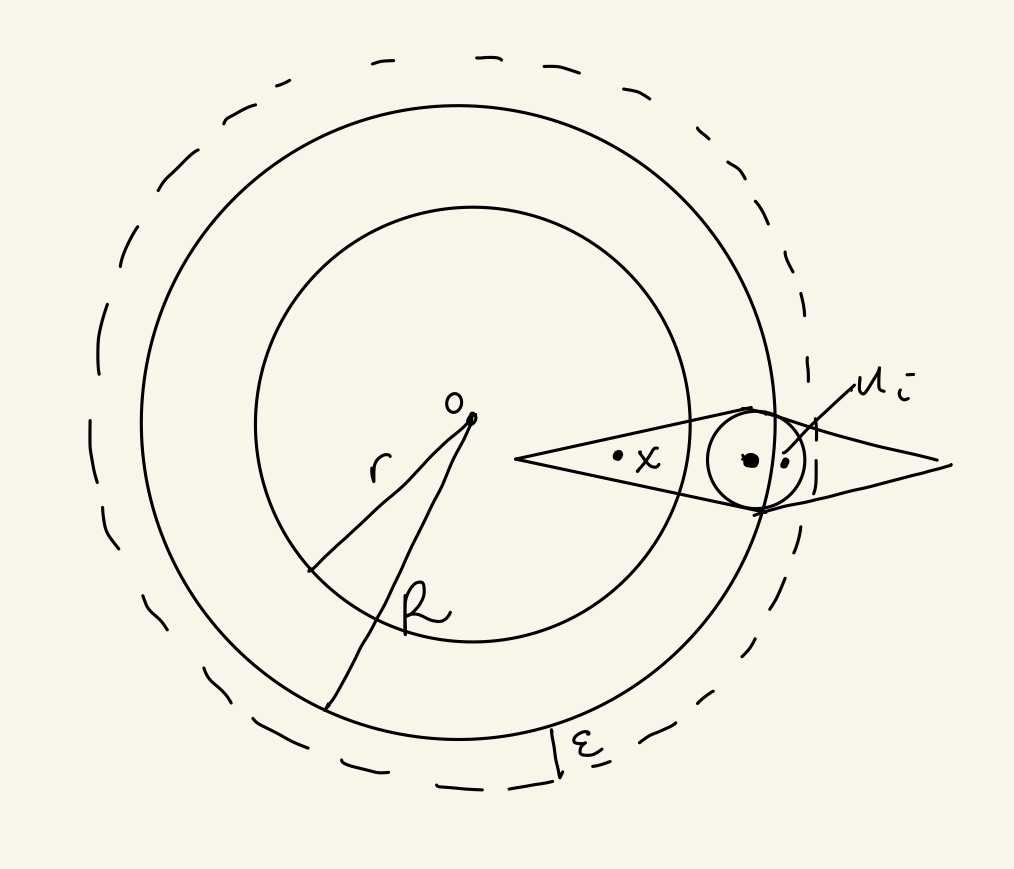
Figure 4. Illustration of partition cell on boundary in the “good” event (A1A2A3A4)csuperscriptsubscript𝐴1subscript𝐴2subscript𝐴3subscript𝐴4𝑐(A_{1}\cup A_{2}\cup A_{3}\cup A_{4})^{c}.

Suppose the event A1cA2cA3cA4csuperscriptsubscript𝐴1𝑐superscriptsubscript𝐴2𝑐superscriptsubscript𝐴3𝑐superscriptsubscript𝐴4𝑐A_{1}^{c}\cap A_{2}^{c}\cap A_{3}^{c}\cap A_{4}^{c} holds. For each xBr𝑥subscript𝐵𝑟x\in B_{r}, this implies that the cell of Y~(M)superscript~𝑌𝑀\tilde{Y}^{(M)} containing x𝑥x has center in BRsubscript𝐵𝑅B_{R}, its inball is contained in BR+εsubscript𝐵𝑅𝜀B_{R+\varepsilon}, and it contains a point ui𝒰subscript𝑢𝑖𝒰u_{i}\in\mathcal{U} such that uixδ8λhmax(Π)normsubscript𝑢𝑖𝑥𝛿8𝜆subscriptΠ\|u_{i}-x\|\leq\frac{\delta}{8\lambda h_{\max}(\Pi)}, see Figure 4. By Corollary 4.1, K(x,y)=e2λh(Π,xy)subscript𝐾𝑥𝑦superscript𝑒2𝜆Π𝑥𝑦K_{\infty}(x,y)=e^{-2\lambda h(\Pi,x-y)}. For x,yBr𝑥𝑦subscript𝐵𝑟x,y\in B_{r}, there are uisubscript𝑢𝑖u_{i} and uj𝒰subscript𝑢𝑗𝒰u_{j}\in\mathcal{U} such that

|K(ui,uj)K(x,y)|subscript𝐾subscript𝑢𝑖subscript𝑢𝑗subscript𝐾𝑥𝑦\displaystyle|K_{\infty}(u_{i},u_{j})-K_{\infty}(x,y)| 2λ|h(Π,uiuj)h(Π,xy)|absent2𝜆Πsubscript𝑢𝑖subscript𝑢𝑗Π𝑥𝑦\displaystyle\leq 2\lambda|h(\Pi,u_{i}-u_{j})-h(\Pi,x-y)|
2λhmax(Π)(uiuj)(xy)absent2𝜆subscriptΠnormsubscript𝑢𝑖subscript𝑢𝑗𝑥𝑦\displaystyle\leq 2\lambda h_{\max}(\Pi)\|(u_{i}-u_{j})-(x-y)\|
2λhmax(Π)(uix+ujy)δ2,absent2𝜆subscriptΠnormsubscript𝑢𝑖𝑥normsubscript𝑢𝑗𝑦𝛿2\displaystyle\leq 2\lambda h_{\max}(\Pi)\left(\|u_{i}-x\|+\|u_{j}-y\|\right)\leq\frac{\delta}{2},

where we have used the inequality |e|x|e|y|||xy|superscript𝑒𝑥superscript𝑒𝑦𝑥𝑦|e^{-|x|}-e^{-|y|}|\leq|x-y| and the subadditivity of the support function. Then, by the assumption A4csuperscriptsubscript𝐴4𝑐A_{4}^{c} and the fact that KMsubscript𝐾𝑀K_{M} is constant over each cell of Y~(M)superscript~𝑌𝑀\tilde{Y}^{(M)},

|KM(x,y)K(x,y)|subscript𝐾𝑀𝑥𝑦subscript𝐾𝑥𝑦\displaystyle|K_{M}(x,y)-K_{\infty}(x,y)|
|KM(x,y)KM(ui,uj)|+|KM(ui,uj)K(ui,uj)|+|K(ui,uj)K(x,y)|absentsubscript𝐾𝑀𝑥𝑦subscript𝐾𝑀subscript𝑢𝑖subscript𝑢𝑗subscript𝐾𝑀subscript𝑢𝑖subscript𝑢𝑗subscript𝐾subscript𝑢𝑖subscript𝑢𝑗subscript𝐾subscript𝑢𝑖subscript𝑢𝑗subscript𝐾𝑥𝑦\displaystyle\leq|K_{M}(x,y)-K_{M}(u_{i},u_{j})|+|K_{M}(u_{i},u_{j})-K_{\infty}(u_{i},u_{j})|+|K_{\infty}(u_{i},u_{j})-K_{\infty}(x,y)|
=|Km(ui,uj)K(ui,uj)|+|K(ui,uj)K(x,y)|δ.absentsubscript𝐾𝑚subscript𝑢𝑖subscript𝑢𝑗subscript𝐾subscript𝑢𝑖subscript𝑢𝑗subscript𝐾subscript𝑢𝑖subscript𝑢𝑗subscript𝐾𝑥𝑦𝛿\displaystyle=|K_{m}(u_{i},u_{j})-K_{\infty}(u_{i},u_{j})|+|K_{\infty}(u_{i},u_{j})-K_{\infty}(x,y)|\leq\delta.

This implies

(supx,yW|KM(x,y)K(x,y)|δ)subscriptsupremum𝑥𝑦𝑊subscript𝐾𝑀𝑥𝑦subscript𝐾𝑥𝑦𝛿\displaystyle\mathbb{P}\left(\sup_{x,y\in W}|K_{M}(x,y)-K_{\infty}(x,y)|\geq\delta\right) (A1A2A3A4).absentsubscript𝐴1subscript𝐴2subscript𝐴3subscript𝐴4\displaystyle\leq\mathbb{P}(A_{1}\cup A_{2}\cup A_{3}\cup A_{4}).

Thus, it remains to prove an upper bound on the probabilities of events Aisubscript𝐴𝑖A_{i}.

We first make the following claim: the typical cell of Y~(M)superscript~𝑌𝑀\tilde{Y}^{(M)}, denoted by Z~~𝑍\tilde{Z}, has the same distribution as the typical cell of a Poisson hyperplane tessellation with mean measure λMΛ()𝜆𝑀Λ\lambda M\Lambda(\cdot). Indeed, let Z0,isubscript𝑍0𝑖Z_{0,i} be the cell of Yisubscript𝑌𝑖Y_{i} containing the origin for each i𝑖i and let Z~~𝑍\tilde{Z} be the zero cell of Y~(M)superscript~𝑌𝑀\tilde{Y}^{(M)}. Then, note that

Z~0=i=1MZ0,i=Z0,1(Z0,1Z0,2)(Z0,1Z0,M),subscript~𝑍0superscriptsubscript𝑖1𝑀subscript𝑍0𝑖subscript𝑍01subscript𝑍01subscript𝑍02subscript𝑍01subscript𝑍0𝑀\displaystyle\tilde{Z}_{0}=\cap_{i=1}^{M}Z_{0,i}=Z_{0,1}\cap(Z_{0,1}\cap Z_{0,2})\cap\cdots(Z_{0,1}\cap\cdots\cap Z_{0,M}),

which implies that Z~0subscript~𝑍0\tilde{Z}_{0} has the same distribution as the zero cell of Y(λM)𝑌𝜆𝑀Y(\lambda M). The claim then follows from Theorem 1 in [40], and the fact that the zero cell of a stationary tessellation determines the distribution of the typical cell (Theorem 10.4.1 in [38]). In particular, this implies 𝔼[V(Z~)]=(Mλ)dV(Π)1𝔼delimited-[]𝑉~𝑍superscript𝑀𝜆𝑑𝑉superscriptΠ1\mathbb{E}[V(\tilde{Z})]=(M\lambda)^{-d}V(\Pi)^{-1} (see [38, (10.44)]).

Now, to bound the probability of A1subscript𝐴1A_{1}, Markov’s inequality and (5) give

(A1)subscript𝐴1\displaystyle\mathbb{P}(A_{1}) 𝔼[CCells(Y~(M))1{c(C)BR}1{CBr}]absent𝔼delimited-[]subscript𝐶Cellssuperscript~𝑌𝑀subscript1𝑐𝐶subscript𝐵𝑅subscript1𝐶subscript𝐵𝑟\displaystyle\leq\mathbb{E}\left[\sum_{C\in\text{Cells}(\tilde{Y}^{(M)})}1_{\{c(C)\notin B_{R}\}}1_{\{C\cap B_{r}\neq\emptyset\}}\right]
=𝔼[V(Z~)]1𝔼[d1{yBR}1{y+Z~Br}dy].absent𝔼superscriptdelimited-[]𝑉~𝑍1𝔼delimited-[]subscriptsuperscript𝑑subscript1𝑦subscript𝐵𝑅subscript1𝑦~𝑍subscript𝐵𝑟differential-d𝑦\displaystyle=\mathbb{E}[V(\tilde{Z})]^{-1}\mathbb{E}\left[\int_{\mathbb{R}^{d}}1_{\{y\notin B_{R}\}}1_{\{y+\tilde{Z}\cap B_{r}\}}\mathrm{d}y\right].

Note that y+Z~Br𝑦~𝑍subscript𝐵𝑟y+\tilde{Z}\cap B_{r}\neq\emptyset if the line segment [y,ryy]𝑦𝑟𝑦norm𝑦[y,r\frac{y}{\|y\|}] is contained in y+Z~𝑦~𝑍y+\tilde{Z}. Then,

(A1)subscript𝐴1\displaystyle\mathbb{P}(A_{1}) 𝔼[V(Z~)]1𝔼[d1{yBR}1{[y,ryy]Z~+y}dy]absent𝔼superscriptdelimited-[]𝑉~𝑍1𝔼delimited-[]subscriptsuperscript𝑑subscript1𝑦subscript𝐵𝑅subscript1𝑦𝑟𝑦norm𝑦~𝑍𝑦differential-d𝑦\displaystyle\leq\mathbb{E}[V(\tilde{Z})]^{-1}\mathbb{E}\left[\int_{\mathbb{R}^{d}}1_{\{y\notin B_{R}\}}1_{\{[y,r\frac{y}{\|y\|}]\subseteq\tilde{Z}+y\}}\mathrm{d}y\right]
=(λM)dV(Π)𝕊d1Rtd1([0,(rt)u]Z~)dtdu.absentsuperscript𝜆𝑀𝑑𝑉Πsubscriptsuperscript𝕊𝑑1superscriptsubscript𝑅superscript𝑡𝑑10𝑟𝑡𝑢~𝑍differential-d𝑡differential-d𝑢\displaystyle=(\lambda M)^{d}V(\Pi)\int_{\mathbb{S}^{d-1}}\int_{R}^{\infty}t^{d-1}\mathbb{P}([0,(r-t)u]\subseteq\tilde{Z})\mathrm{d}t\mathrm{d}u.

By Corollary 10.4.1 in [38] and our claim about the distribution of Z~0subscript~𝑍0\tilde{Z}_{0},

([0,(rt)u]Z~)([0,(rt)u]Z~0)=eλM(tr)h(Π,u),0𝑟𝑡𝑢~𝑍0𝑟𝑡𝑢subscript~𝑍0superscript𝑒𝜆𝑀𝑡𝑟Π𝑢\displaystyle\mathbb{P}([0,(r-t)u]\subseteq\tilde{Z})\leq\mathbb{P}([0,(r-t)u]\subseteq\tilde{Z}_{0})=e^{-\lambda M(t-r)h(\Pi,u)},

Then,

(A1)subscript𝐴1\displaystyle\mathbb{P}(A_{1}) (λM)dV(Π)𝕊d1Rtd1eλM(tr)h(Π,u)dtduabsentsuperscript𝜆𝑀𝑑𝑉Πsubscriptsuperscript𝕊𝑑1superscriptsubscript𝑅superscript𝑡𝑑1superscript𝑒𝜆𝑀𝑡𝑟Π𝑢differential-d𝑡differential-d𝑢\displaystyle\leq(\lambda M)^{d}V(\Pi)\int_{\mathbb{S}^{d-1}}\int_{R}^{\infty}t^{d-1}e^{-\lambda M(t-r)h(\Pi,u)}\mathrm{d}t\mathrm{d}u
(λM)dV(Π)dκdRtd1eλM(tr)hmin(Π)dtabsentsuperscript𝜆𝑀𝑑𝑉Π𝑑subscript𝜅𝑑superscriptsubscript𝑅superscript𝑡𝑑1superscript𝑒𝜆𝑀𝑡𝑟subscriptΠdifferential-d𝑡\displaystyle\leq(\lambda M)^{d}V(\Pi)d\kappa_{d}\int_{R}^{\infty}t^{d-1}e^{-\lambda M(t-r)h_{\min}(\Pi)}\mathrm{d}t
=(λM)dV(Π)dκd(λMhmin(Π))deλMhmin(Π)rλMhmin(Π)Rxd1exdxabsentsuperscript𝜆𝑀𝑑𝑉Π𝑑subscript𝜅𝑑superscript𝜆𝑀subscriptΠ𝑑superscript𝑒𝜆𝑀subscriptΠ𝑟superscriptsubscript𝜆𝑀subscriptΠ𝑅superscript𝑥𝑑1superscript𝑒𝑥differential-d𝑥\displaystyle=(\lambda M)^{d}V(\Pi)d\kappa_{d}(\lambda Mh_{\min}(\Pi))^{-d}e^{\lambda Mh_{\min}(\Pi)r}\int_{\lambda Mh_{\min}(\Pi)R}^{\infty}x^{d-1}e^{-x}\mathrm{d}x
V(Π)dκdhmin(Π)deλMhmin(Π)rΓ(d)[1(1eλMhmin(Π)RΓ(d+1)1/d)d]absent𝑉Π𝑑subscript𝜅𝑑subscriptsuperscriptΠ𝑑superscript𝑒𝜆𝑀subscriptΠ𝑟Γ𝑑delimited-[]1superscript1superscript𝑒𝜆𝑀subscriptΠ𝑅Γsuperscript𝑑11𝑑𝑑\displaystyle\leq V(\Pi)d\kappa_{d}h_{\min}(\Pi)^{-d}e^{\lambda Mh_{\min}(\Pi)r}\Gamma(d)\left[1-\left(1-e^{-\frac{\lambda Mh_{\min}(\Pi)R}{\Gamma(d+1)^{1/d}}}\right)^{d}\right]
V(Π)dκdhmin(Π)dΓ(d+1)eλMhmin(Π)(RΓ(d+1)1/dr).absent𝑉Π𝑑subscript𝜅𝑑subscriptsuperscriptΠ𝑑Γ𝑑1superscript𝑒𝜆𝑀subscriptΠ𝑅Γsuperscript𝑑11𝑑𝑟\displaystyle\leq V(\Pi)d\kappa_{d}h_{\min}(\Pi)^{-d}\Gamma(d+1)e^{-\lambda Mh_{\min}(\Pi)\left(R\Gamma(d+1)^{-1/d}-r\right)}.

where the second to last inequality follows from [1, Theorem 1] and the last inequality from the fact that (1ex)d1dex1superscript𝑒𝑥𝑑1𝑑superscript𝑒𝑥(1-e^{-x})d\geq 1-de^{-x} for x>0𝑥0x>0.

To bound the probability of A2subscript𝐴2A_{2}, note that A2subscript𝐴2A_{2} implies there is a cell of Y~(M)superscript~𝑌𝑀\tilde{Y}^{(M)} with center in BRsubscript𝐵𝑅B_{R} such that the largest ball contained in the cell has radius smaller than ε𝜀\varepsilon. That is, there is a cell with inradius smaller that ε𝜀\varepsilon. Indeed, if all cells had this property, then all cells would contain a point of 𝒰𝒰\mathcal{U}. By Markov’s inequality, (5), and Theorem 10.4.8 in [38],

(A2)subscript𝐴2\displaystyle\mathbb{P}(A_{2}) 𝔼[CCells(Y~(M))1{r(C)ε}1{c(C)BR}]absent𝔼delimited-[]subscript𝐶Cellssuperscript~𝑌𝑀subscript1𝑟𝐶𝜀subscript1𝑐𝐶subscript𝐵𝑅\displaystyle\leq\mathbb{E}\left[\sum_{C\in\mathrm{Cells}(\tilde{Y}^{(M)})}1_{\{r(C)\leq\varepsilon\}}1_{\{c(C)\in B_{R}\}}\right]
=𝔼[V(Z~)]1𝔼[d1{r(Z~+y)ε}1{yBR}dy]absent𝔼superscriptdelimited-[]𝑉~𝑍1𝔼delimited-[]subscriptsuperscript𝑑subscript1𝑟~𝑍𝑦𝜀subscript1𝑦subscript𝐵𝑅differential-d𝑦\displaystyle=\mathbb{E}[V(\tilde{Z})]^{-1}\mathbb{E}\left[\int_{\mathbb{R}^{d}}1_{\{r(\tilde{Z}+y)\leq\varepsilon\}}1_{\{y\in B_{R}\}}\mathrm{d}y\right]
=(λM)dV(Π)V(BR)(r(Z~)ε)absentsuperscript𝜆𝑀𝑑𝑉Π𝑉subscript𝐵𝑅𝑟~𝑍𝜀\displaystyle=(\lambda M)^{d}V(\Pi)V(B_{R})\mathbb{P}(r(\tilde{Z})\leq\varepsilon)
(λM)dV(Π)V(BR)(1e2Mλε).absentsuperscript𝜆𝑀𝑑𝑉Π𝑉subscript𝐵𝑅1superscript𝑒2𝑀𝜆𝜀\displaystyle\leq(\lambda M)^{d}V(\Pi)V(B_{R})(1-e^{-2M\lambda\varepsilon}).

Also by Markov’s inequality and (5),

(A3)subscript𝐴3\displaystyle\mathbb{P}(A_{3}) 𝔼[Ccells(Y~(M))1{Diam(C)δ8λh(Π,umax)}1{c(C)BR}]absent𝔼delimited-[]subscript𝐶cellssuperscript~𝑌𝑀subscript1Diam𝐶𝛿8𝜆Πsubscript𝑢subscript1𝑐𝐶subscript𝐵𝑅\displaystyle\leq\mathbb{E}\left[\sum_{C\in\mathrm{cells}(\tilde{Y}^{(M)})}1_{\{\text{Diam}(C)\geq\frac{\delta}{8\lambda h(\Pi,u_{\max})}\}}1_{\{c(C)\in B_{R}\}}\right]
=𝔼[V(Z~)]1V(BR)(Diam(Z~)δ8λhmax(Π)).absent𝔼superscriptdelimited-[]𝑉~𝑍1𝑉subscript𝐵𝑅Diam~𝑍𝛿8𝜆subscriptΠ\displaystyle=\mathbb{E}[V(\tilde{Z})]^{-1}V(B_{R})\mathbb{P}\left(\text{Diam}(\tilde{Z})\geq\frac{\delta}{8\lambda h_{\max}(\Pi)}\right).

Then, by the proof of Theorem 2 in section 8 of [18], for any fixed τ(0,1)𝜏01\tau\in(0,1),

(12) (Diam(Z~)δ8λhmax(Π))c0eMτδhmin(Π)8hmax(Π),Diam~𝑍𝛿8𝜆subscriptΠsubscript𝑐0superscript𝑒𝑀𝜏𝛿subscriptΠ8subscriptΠ\displaystyle\mathbb{P}\left(\text{Diam}(\tilde{Z})\geq\frac{\delta}{8\lambda h_{\max}(\Pi)}\right)\leq c_{0}e^{-M\frac{\tau\delta h_{\min}(\Pi)}{8h_{\max}(\Pi)}},

where c0=c0(τ,Π,δ)subscript𝑐0subscript𝑐0𝜏Π𝛿c_{0}=c_{0}(\tau,\Pi,\delta) and thus

(A3)subscript𝐴3\displaystyle\mathbb{P}(A_{3}) c0(λM)dV(Π)V(BR)eMδτhmin(Π)8hmax(Π).absentsubscript𝑐0superscript𝜆𝑀𝑑𝑉Π𝑉subscript𝐵𝑅superscript𝑒𝑀𝛿𝜏subscriptΠ8subscriptΠ\displaystyle\leq c_{0}(\lambda M)^{d}V(\Pi)V(B_{R})e^{-M\frac{\delta\tau h_{\min}(\Pi)}{8h_{\max}(\Pi)}}.

Finally, to bound the probability of A4subscript𝐴4A_{4}, one can choose a ε𝜀\varepsilon-covering 𝒰𝒰\mathcal{U} of size at most (6(R+ε)ε)dsuperscript6𝑅𝜀𝜀𝑑\left(\frac{6(R+\varepsilon)}{\varepsilon}\right)^{d}, see Lemma 4.1 in [33]. A union bound and Hoeffding’s inequality gives

(A4)subscript𝐴4\displaystyle\mathbb{P}(A_{4}) i,j𝒰(|KM(ui,uj)K(ui,uj)|>δ2)=(6(R+ε)ε)2d2eMδ2/2.absentsubscript𝑖𝑗𝒰subscript𝐾𝑀subscript𝑢𝑖subscript𝑢𝑗subscript𝐾subscript𝑢𝑖subscript𝑢𝑗𝛿2superscript6𝑅𝜀𝜀2𝑑2superscript𝑒𝑀superscript𝛿22\displaystyle\leq\sum_{i,j\in\mathcal{U}}\mathbb{P}\left(|K_{M}(u_{i},u_{j})-K_{\infty}(u_{i},u_{j})|>\frac{\delta}{2}\right)=\left(\frac{6(R+\varepsilon)}{\varepsilon}\right)^{2d}2e^{-M\delta^{2}/2}.

For all ε>0𝜀0\varepsilon>0 small enough, putting these bounds together and using the bound 1exx1superscript𝑒𝑥𝑥1-e^{-x}\leq x, we obtain, for all M𝑀M large enough,

(A1A2A3A4)i=14(Ai)subscript𝐴1subscript𝐴2subscript𝐴3subscript𝐴4superscriptsubscript𝑖14subscript𝐴𝑖\displaystyle\mathbb{P}(A_{1}\cup A_{2}\cup A_{3}\cup A_{4})\leq\sum_{i=1}^{4}\mathbb{P}(A_{i})
c1Md1Rd1(eλMhmin(Π)(RΓ(d+1)1/dr)+MReMδτhmin(Π)8hmax(Π))absentsubscript𝑐1superscript𝑀𝑑1superscript𝑅𝑑1superscript𝑒𝜆𝑀subscriptΠ𝑅Γsuperscript𝑑11𝑑𝑟𝑀𝑅superscript𝑒𝑀𝛿𝜏subscriptΠ8subscriptΠ\displaystyle\leq c_{1}M^{d-1}R^{d-1}\left(e^{-\lambda Mh_{\min}(\Pi)(R\Gamma(d+1)^{-1/d}-r)}+MRe^{-M\frac{\delta\tau h_{\min}(\Pi)}{8h_{\max}(\Pi)}}\right)
+c2RdMd+1ε+c3ε2deMδ2/2,subscript𝑐2superscript𝑅𝑑superscript𝑀𝑑1𝜀subscript𝑐3superscript𝜀2𝑑superscript𝑒𝑀superscript𝛿22\displaystyle\qquad\qquad+c_{2}R^{d}M^{d+1}\varepsilon+c_{3}\varepsilon^{-2d}e^{-M\delta^{2}/2},

where the constants cisubscript𝑐𝑖c_{i} are all positive and depend on δ𝛿\delta, τ𝜏\tau, λ𝜆\lambda, d𝑑d, r𝑟r, and ΠΠ\Pi. Differentiating with respect to ε𝜀\varepsilon and setting equal to zero, the above upper bound hits a minimum at

ε0=c4Md+12d+1Rd2d+1eMδ24d+2.subscript𝜀0subscript𝑐4superscript𝑀𝑑12𝑑1superscript𝑅𝑑2𝑑1superscript𝑒𝑀superscript𝛿24𝑑2\displaystyle\varepsilon_{0}=c_{4}M^{-\frac{d+1}{2d+1}}R^{-\frac{d}{2d+1}}e^{-\frac{M\delta^{2}}{4d+2}}.

Thus, since the above bound holds for any ε>0𝜀0\varepsilon>0,

(A1A2A3A4)subscript𝐴1subscript𝐴2subscript𝐴3subscript𝐴4\displaystyle\mathbb{P}(A_{1}\cup A_{2}\cup A_{3}\cup A_{4})
c1Md1Rd1(eλMhmin(Π)(RΓ(d+1)1/dr)+MReMδτhmin(Π)8hmax)absentsubscript𝑐1superscript𝑀𝑑1superscript𝑅𝑑1superscript𝑒𝜆𝑀subscriptΠ𝑅Γsuperscript𝑑11𝑑𝑟𝑀𝑅superscript𝑒𝑀𝛿𝜏subscriptΠ8subscript\displaystyle\leq c_{1}M^{d-1}R^{d-1}\left(e^{-\lambda Mh_{\min}(\Pi)(R\Gamma(d+1)^{-1/d}-r)}+MRe^{-M\frac{\delta\tau h_{\min}(\Pi)}{8h_{\max}}}\right)
+c5Rdd2d+1Md+1d+12d+1eMδ24d+2+c6M2d(d+1)2d+1R2d22d+1e2dMδ24d+2Mδ22subscript𝑐5superscript𝑅𝑑𝑑2𝑑1superscript𝑀𝑑1𝑑12𝑑1superscript𝑒𝑀superscript𝛿24𝑑2subscript𝑐6superscript𝑀2𝑑𝑑12𝑑1superscript𝑅2superscript𝑑22𝑑1superscript𝑒2𝑑𝑀superscript𝛿24𝑑2𝑀superscript𝛿22\displaystyle\qquad\qquad+c_{5}R^{d-\frac{d}{2d+1}}M^{d+1-\frac{d+1}{2d+1}}e^{-\frac{M\delta^{2}}{4d+2}}+c_{6}M^{\frac{2d(d+1)}{2d+1}}R^{\frac{2d^{2}}{2d+1}}e^{\frac{2dM\delta^{2}}{4d+2}-\frac{M\delta^{2}}{2}}
c1Md1Rd1eλMhmin(Π)(RΓ(d+1)1/dr)+c1MdRdeMδτhmin(Π)8hmax(Π)absentsubscript𝑐1superscript𝑀𝑑1superscript𝑅𝑑1superscript𝑒𝜆𝑀subscriptΠ𝑅Γsuperscript𝑑11𝑑𝑟subscript𝑐1superscript𝑀𝑑superscript𝑅𝑑superscript𝑒𝑀𝛿𝜏subscriptΠ8subscriptΠ\displaystyle\leq c_{1}M^{d-1}R^{d-1}e^{-\lambda Mh_{\min}(\Pi)(R\Gamma(d+1)^{-1/d}-r)}+c_{1}M^{d}R^{d}e^{-M\frac{\delta\tau h_{\min}(\Pi)}{8h_{\max}(\Pi)}}
+c7R2d22d+1Md+d2d+1eMδ24d+2.subscript𝑐7superscript𝑅2superscript𝑑22𝑑1superscript𝑀𝑑𝑑2𝑑1superscript𝑒𝑀superscript𝛿24𝑑2\displaystyle\qquad\qquad+c_{7}R^{\frac{2d^{2}}{2d+1}}M^{d+\frac{d}{2d+1}}e^{-\frac{M\delta^{2}}{4d+2}}.

Finally, letting R=Γ(d+1)1/d(r+δ2λhmin(Π)(4d+2))𝑅Γsuperscript𝑑11𝑑𝑟superscript𝛿2𝜆subscriptΠ4𝑑2R=\Gamma(d+1)^{1/d}\left(r+\frac{\delta^{2}}{\lambda h_{\min}(\Pi)(4d+2)}\right) gives: for any fixed τ(0,1)𝜏01\tau\in(0,1)

(A1A2A3A4)subscript𝐴1subscript𝐴2subscript𝐴3subscript𝐴4\displaystyle\mathbb{P}(A_{1}\cup A_{2}\cup A_{3}\cup A_{4}) c8Md+d2d+1eMmin{δτhmin(Π)8hmax(Π),δ24d+2}.absentsubscript𝑐8superscript𝑀𝑑𝑑2𝑑1superscript𝑒𝑀𝛿𝜏subscriptΠ8subscriptΠsuperscript𝛿24𝑑2\displaystyle\leq c_{8}M^{d+\frac{d}{2d+1}}e^{-M\min\left\{\frac{\delta\tau h_{\min}(\Pi)}{8h_{\max}(\Pi)},\frac{\delta^{2}}{4d+2}\right\}}.

Remark 4.1.

While Theorem 4.3 gives the rate of convergence with respect to the number of STIT partitions M𝑀M in the approximation, the constant C𝐶C in the upper bound that depends on δ𝛿\delta, W𝑊W, τ𝜏\tau, and d𝑑d cannot be written explicitly from our proof. This is due to the constant in the tail bound of the diameter of the typical cell (12). We leave for future work a more explicit and optimal tail bound for the diameter, see open questions in section 6.

5. Density estimation with STIT forests

Let λ>0𝜆0\lambda>0 and consider a STIT tessellation Y(λd)𝑌𝜆𝑑Y(\lambda d) with associated intensity measure ΛΛ\Lambda and denote by Zxλsubscriptsuperscript𝑍𝜆𝑥Z^{\lambda}_{x} the cell of Y(λd)𝑌𝜆𝑑Y(\lambda d) containing xd𝑥superscript𝑑x\in\mathbb{R}^{d}. We consider lifetimes scaling with dimension d𝑑d so as to better compare with Laplace kernel density estimation. Indeed, Theorem 4.1 shows that sampling from Y(d)𝑌𝑑Y(d) approximates the Laplace kernel when ΛΛ\Lambda is as in (4).

Let X1,,Xnsubscript𝑋1subscript𝑋𝑛X_{1},\ldots,X_{n} be n𝑛n i.i.d. points drawn from a distribution with unknown density f𝑓f. Define the density estimator for f𝑓f from a single STIT tree as

fλ,n(x):=1ni=1n1{xZXiλ}V(ZXiλ)=1ni=1n1{XiZxλ}V(Zxλ),assignsubscript𝑓𝜆𝑛𝑥1𝑛superscriptsubscript𝑖1𝑛subscript1𝑥subscriptsuperscript𝑍𝜆subscript𝑋𝑖𝑉subscriptsuperscript𝑍𝜆subscript𝑋𝑖1𝑛superscriptsubscript𝑖1𝑛subscript1subscript𝑋𝑖subscriptsuperscript𝑍𝜆𝑥𝑉subscriptsuperscript𝑍𝜆𝑥f_{\lambda,n}(x):=\frac{1}{n}\sum_{i=1}^{n}\frac{1_{\{x\in Z^{\lambda}_{X_{i}}\}}}{V(Z^{\lambda}_{X_{i}})}=\frac{1}{n}\sum_{i=1}^{n}\frac{1_{\{X_{i}\in Z^{\lambda}_{x}\}}}{V(Z^{\lambda}_{x})},

where V(Z)𝑉𝑍V(Z) denotes the volume of a cell Z𝑍Z. Dividing by the volumes ensures that fn(x)subscript𝑓𝑛𝑥f_{n}(x) integrates to one, that is, it is indeed a density. Similarly, define the density estimator for f𝑓f from a STIT forest with M𝑀M i.i.d. trees as

(13) fλ,n,M(x):=1Mm=1Mfn(m)(x),assignsubscript𝑓𝜆𝑛𝑀𝑥1𝑀superscriptsubscript𝑚1𝑀superscriptsubscript𝑓𝑛𝑚𝑥\displaystyle f_{\lambda,n,M}(x):=\frac{1}{M}\sum_{m=1}^{M}f_{n}^{(m)}(x),

where {fλ,n(m)}m=1Msuperscriptsubscriptsuperscriptsubscript𝑓𝜆𝑛𝑚𝑚1𝑀\{f_{\lambda,n}^{(m)}\}_{m=1}^{M} are i.i.d. copies of the estimator fλ,nsubscript𝑓𝜆𝑛f_{\lambda,n} obtained from M𝑀M i.i.d. copies of the STIT tessellation Y1,,YMsubscript𝑌1subscript𝑌𝑀Y_{1},\ldots,Y_{M}. By the strong law of large numbers, as M𝑀M\to\infty,

fλ,n,M(x)fλ,n,(x):=𝔼[fn(x)],a.s.formulae-sequencesubscript𝑓𝜆𝑛𝑀𝑥subscript𝑓𝜆𝑛𝑥assign𝔼delimited-[]subscript𝑓𝑛𝑥𝑎𝑠f_{\lambda,n,M}(x)\to f_{\lambda,n,\infty}(x):=\mathbb{E}\left[f_{n}(x)\right],\qquad a.s.

We first show that the ideal STIT forest estimator fλ,n,subscript𝑓𝜆𝑛f_{\lambda,n,\infty} is always a kernel estimator for any stationary measure ΛΛ\Lambda. Then, in our last main result (cf. Theorem 5.1) we will derive the explicit formula for the Mondrian forest.

Proposition 5.1.

In the above settings,

(14) fλ,n,(x)=λdni=1nK0,Λ(λ(xXi)),subscript𝑓𝜆𝑛𝑥superscript𝜆𝑑𝑛superscriptsubscript𝑖1𝑛subscript𝐾0Λ𝜆𝑥subscript𝑋𝑖\displaystyle f_{\lambda,n,\infty}(x)=\frac{\lambda^{d}}{n}\sum_{i=1}^{n}K_{0,\Lambda}(\lambda(x-X_{i})),

where

K0,Λ(x):=𝔼[1{xZ0}V(Z0)],assignsubscript𝐾0Λ𝑥𝔼delimited-[]subscript1𝑥subscript𝑍0𝑉subscript𝑍0K_{0,\Lambda}(x):=\mathbb{E}\left[\frac{1_{\{x\in Z_{0}\}}}{V(Z_{0})}\right],

and Z0subscript𝑍0Z_{0} is the zero cell of Y(d)𝑌𝑑Y(d), i.e. the cell of Y(d)𝑌𝑑Y(d) containing the origin. That is, the ideal STIT forest density estimator (with infinitely many trees) is a kernel density estimator with kernel K0,Λsubscript𝐾0ΛK_{0,\Lambda} and bandwidth λ1superscript𝜆1\lambda^{-1}.

Proof.

First, note that K0,Λsubscript𝐾0ΛK_{0,\Lambda} is symmetric and K0,Λ(x)dx=1subscript𝐾0Λ𝑥differential-d𝑥1\int K_{0,\Lambda}(x)\mathrm{d}x=1. Also, for λ>0𝜆0\lambda>0, define

K0,Λλ(x):=𝔼[1{xZ0λ}V(Z0λ)]=𝔼[1{λxZ0}λdV(Z0)]=λdK0,Λ(λx),assignsuperscriptsubscript𝐾0Λ𝜆𝑥𝔼delimited-[]subscript1𝑥subscriptsuperscript𝑍𝜆0𝑉subscriptsuperscript𝑍𝜆0𝔼delimited-[]subscript1𝜆𝑥subscript𝑍0superscript𝜆𝑑𝑉subscript𝑍0superscript𝜆𝑑subscript𝐾0Λ𝜆𝑥K_{0,\Lambda}^{\lambda}(x):=\mathbb{E}\left[\frac{1_{\{x\in Z^{\lambda}_{0}\}}}{V(Z^{\lambda}_{0})}\right]=\mathbb{E}\left[\frac{1_{\{\lambda x\in Z_{0}\}}}{\lambda^{-d}V(Z_{0})}\right]=\lambda^{d}K_{0,\Lambda}(\lambda x),

where the equalities follow from the self-similarity property of the STIT tessellation. By stationarity, for all x,yd𝑥𝑦superscript𝑑x,y\in\mathbb{R}^{d}, 𝔼[1{xZy}V(Zy)]=𝔼[1{xyZ0}V(Z0)]𝔼delimited-[]subscript1𝑥subscript𝑍𝑦𝑉subscript𝑍𝑦𝔼delimited-[]subscript1𝑥𝑦subscript𝑍0𝑉subscript𝑍0\mathbb{E}\left[\frac{1_{\{x\in Z_{y}\}}}{V(Z_{y})}\right]=\mathbb{E}\left[\frac{1_{\{x-y\in Z_{0}\}}}{V(Z_{0})}\right]. Thus,

fλ,n,(x)=𝔼[fλ,n(x)]=1ni=1n𝔼[1{XiZxλ}V(Zxλ)]=K0,Λλ(xXi),subscript𝑓𝜆𝑛𝑥𝔼delimited-[]subscript𝑓𝜆𝑛𝑥1𝑛superscriptsubscript𝑖1𝑛𝔼delimited-[]subscript1subscript𝑋𝑖superscriptsubscript𝑍𝑥𝜆𝑉superscriptsubscript𝑍𝑥𝜆subscriptsuperscript𝐾𝜆0Λ𝑥subscript𝑋𝑖f_{\lambda,n,\infty}(x)=\mathbb{E}[f_{\lambda,n}(x)]=\frac{1}{n}\sum_{i=1}^{n}\mathbb{E}\left[\frac{1_{\{X_{i}\in Z_{x}^{\lambda}\}}}{V(Z_{x}^{\lambda})}\right]=K^{\lambda}_{0,\Lambda}(x-X_{i}),

and we obtain (14). ∎

One may guess that this limiting kernel K0λsubscriptsuperscript𝐾𝜆0K^{\lambda}_{0} is just the STIT kernel Ksubscript𝐾K_{\infty} of Theorem 4.1. However, already for the Mondrian case, this is not true. This difference was discussed in [3] in the context of regression. Our next main result, Theorem 5.1, makes precise the limiting behavior of the Mondrian forest density estimator. In particular, the limiting density estimator fλ,n,subscript𝑓𝜆𝑛f_{\lambda,n,\infty} of the Mondrian forest is revealed to be a kernel estimator with a Laplace component and a volume correction term.

Theorem 5.1.

Consider n𝑛n i.i.d. points X1,,Xnsubscript𝑋1subscript𝑋𝑛X_{1},\ldots,X_{n} drawn from a distribution with unknown density f𝑓f. Let λ>0𝜆0\lambda>0, and let fλ,n,Msubscript𝑓𝜆𝑛𝑀f_{\lambda,n,M} denote the random forest estimator as in (13) obtained from running M𝑀M independent Mondrian processes, i.e. STIT processes with ΛΛ\Lambda as in (4). Let fλ,n,subscript𝑓𝜆𝑛f_{\lambda,n,\infty} denote the ideal forest estimator (obtained with infinitely many trees) in this case. Then,

fλ,n,(x)=λdni=1neλxXi1j=1dh(λ|xjXi(j)|),subscript𝑓𝜆𝑛𝑥superscript𝜆𝑑𝑛superscriptsubscript𝑖1𝑛superscript𝑒𝜆subscriptnorm𝑥subscript𝑋𝑖1superscriptsubscriptproduct𝑗1𝑑𝜆subscript𝑥𝑗superscriptsubscript𝑋𝑖𝑗\displaystyle f_{\lambda,n,\infty}(x)=\frac{\lambda^{d}}{n}\sum_{i=1}^{n}e^{-\lambda\|x-X_{i}\|_{1}}\prod_{j=1}^{d}h\left(\lambda|x_{j}-X_{i}^{(j)}|\right),

where h(t):=1tetE1(t)assign𝑡1𝑡superscript𝑒𝑡subscript𝐸1𝑡h(t):=1-te^{t}E_{1}(t) and E1()subscript𝐸1E_{1}(\cdot) is the exponential integral E1(t):=tessdsassignsubscript𝐸1𝑡superscriptsubscript𝑡superscript𝑒𝑠𝑠differential-d𝑠E_{1}(t):=\int_{t}^{\infty}\frac{e^{-s}}{s}\mathrm{d}s.

Corollary 5.1.

In the setting of Theorem 5.1, the density estimator fλ,n,Msubscript𝑓𝜆𝑛𝑀f_{\lambda,n,M} is a random approximation of the kernel density estimator fλ,n,subscript𝑓𝜆𝑛f_{\lambda,n,\infty} corresponding to a bandwidth λ1superscript𝜆1\lambda^{-1} and kernel

(15) K0(x)=ex1j=1dh(|xj|).subscript𝐾0𝑥superscript𝑒subscriptnorm𝑥1superscriptsubscriptproduct𝑗1𝑑subscript𝑥𝑗K_{0}(x)=e^{-\|x\|_{1}}\prod_{j=1}^{d}h(|x_{j}|).

Note that the first term ex1superscript𝑒subscriptnorm𝑥1e^{-\|x\|_{1}} of K0subscript𝐾0K_{0} is the Laplace kernel, and the second term decays as x𝑥x gets farther from the origin. In other words, the kernel of the infinite Mondrian forest decays faster from the observed points compared to the Laplace kernel. This can be seen clearly in Figure 2. Recall that the Laplace kernel density estimator for a density f𝑓f given i.i.d. draws X1,,Xnsubscript𝑋1subscript𝑋𝑛X_{1},\ldots,X_{n} and bandwidth λ1superscript𝜆1\lambda^{-1} is given by

f^λ,n(x)=1n(λ2)di=1neλxXi1.subscript^𝑓𝜆𝑛𝑥1𝑛superscript𝜆2𝑑superscriptsubscript𝑖1𝑛superscript𝑒𝜆subscriptnorm𝑥subscript𝑋𝑖1\hat{f}_{\lambda,n}(x)=\frac{1}{n}\left(\frac{\lambda}{2}\right)^{d}\sum_{i=1}^{n}e^{-\lambda\|x-X_{i}\|_{1}}.

Comparing this estimator with fλ,n,subscript𝑓𝜆𝑛f_{\lambda,n,\infty} shows that fλ,n,subscript𝑓𝜆𝑛f_{\lambda,n,\infty} is a more data-biased version of the Laplace kernel, as discussed in the introduction. Starting from M𝑀M samples of the STIT tessellation Y(λd)𝑌𝜆𝑑Y(\lambda d), the following density estimator for a density f𝑓f can also be considered. For xd𝑥superscript𝑑x\in\mathbb{R}^{d}, define

f^λ,n,M(x)=1ni=1n1Mm=1M1{XiZxλ}1Mm=1MV(Zxλ).subscript^𝑓𝜆𝑛𝑀𝑥1𝑛superscriptsubscript𝑖1𝑛1𝑀superscriptsubscript𝑚1𝑀subscript1subscript𝑋𝑖subscriptsuperscript𝑍𝜆𝑥1𝑀superscriptsubscript𝑚1𝑀𝑉subscriptsuperscript𝑍𝜆𝑥\hat{f}_{\lambda,n,M}(x)=\frac{1}{n}\sum_{i=1}^{n}\frac{\frac{1}{M}\sum_{m=1}^{M}1_{\{X_{i}\in Z^{\lambda}_{x}\}}}{\frac{1}{M}\sum_{m=1}^{M}V(Z^{\lambda}_{x})}.

This estimator is a Monte Carlo estimate for the the Laplace kernel density estimator.

Proof of Theorem 5.1.

Following from Proposition 5.1, it remains to compute K0,Λsubscript𝐾0ΛK_{0,\Lambda} explicitly for the Mondrian process. In this case, we will denote the kernel by K0subscript𝐾0K_{0}. By [28, Proposition 1], the zero cell Z0subscript𝑍0Z_{0} of the Mondrian process Y(d)𝑌𝑑Y(d) has the distribution

(16) Z0λ=Dj=1d[Tj,0,Tj,1]subscriptsuperscript𝑍𝜆0Dsuperscriptsubscriptproduct𝑗1𝑑subscript𝑇𝑗0subscript𝑇𝑗1\displaystyle Z^{\lambda}_{0}\overset{\mathrm{D}}{=}\prod_{j=1}^{d}[-T_{j,0},T_{j,1}]

where {Tj,k}j=1,,d;k=0,1subscriptsubscript𝑇𝑗𝑘formulae-sequence𝑗1𝑑𝑘01\{T_{j,k}\}_{j=1,\ldots,d;k=0,1} are i.i.d. exponential random variables with parameter 111. Then,

K0(x)=𝔼[1{xZ0}V(Z0)]subscript𝐾0𝑥𝔼delimited-[]subscript1𝑥subscript𝑍0𝑉subscript𝑍0\displaystyle K_{0}(x)=\mathbb{E}\left[\frac{1_{\{x\in Z_{0}\}}}{V(Z_{0})}\right] =j=1d(𝔼[1{0xjTj,1}Tj,0+Tj,1]+𝔼[1{Tj,0xj0}Tj,0+Tj,1])absentsuperscriptsubscriptproduct𝑗1𝑑𝔼delimited-[]subscript10subscript𝑥𝑗subscript𝑇𝑗1subscript𝑇𝑗0subscript𝑇𝑗1𝔼delimited-[]subscript1subscript𝑇𝑗0subscript𝑥𝑗0subscript𝑇𝑗0subscript𝑇𝑗1\displaystyle=\prod_{j=1}^{d}\left(\mathbb{E}\left[\frac{1_{\{0\leq x_{j}\leq T_{j,1}\}}}{T_{j,0}+T_{j,1}}\right]+\mathbb{E}\left[\frac{1_{\{-T_{j,0}\leq x_{j}\leq 0\}}}{T_{j,0}+T_{j,1}}\right]\right)
=j=1d𝔼[1{|xj|T0}T0+T1].absentsuperscriptsubscriptproduct𝑗1𝑑𝔼delimited-[]subscript1subscript𝑥𝑗subscript𝑇0subscript𝑇0subscript𝑇1\displaystyle=\prod_{j=1}^{d}\mathbb{E}\left[\frac{1_{\{|x_{j}|\leq T_{0}\}}}{T_{0}+T_{1}}\right].

By the change of variable z=t+s𝑧𝑡𝑠z=t+s,

𝔼[1{|x|T0}T0+T1]=001{|x|t}e(t+s)t+sdtds=0s1{|x|zs}ezzdzds𝔼delimited-[]subscript1𝑥subscript𝑇0subscript𝑇0subscript𝑇1superscriptsubscript0superscriptsubscript0subscript1𝑥𝑡superscript𝑒𝑡𝑠𝑡𝑠differential-d𝑡differential-d𝑠superscriptsubscript0superscriptsubscript𝑠subscript1𝑥𝑧𝑠superscript𝑒𝑧𝑧differential-d𝑧differential-d𝑠\displaystyle\mathbb{E}\left[\frac{1_{\{|x|\leq T_{0}\}}}{T_{0}+T_{1}}\right]=\int_{0}^{\infty}\int_{0}^{\infty}1_{\{|x|\leq t\}}\frac{e^{-(t+s)}}{t+s}\mathrm{d}t\mathrm{d}s=\int_{0}^{\infty}\int_{s}^{\infty}1_{\{|x|\leq z-s\}}\frac{e^{-z}}{z}\mathrm{d}z\mathrm{d}s
=0ezz(01{sz}1{sz|x|}ds)dz=01{z|x|}(zz|x|z)ezdzabsentsuperscriptsubscript0superscript𝑒𝑧𝑧superscriptsubscript0subscript1𝑠𝑧subscript1𝑠𝑧𝑥differential-d𝑠differential-d𝑧superscriptsubscript0subscript1𝑧𝑥𝑧𝑧𝑥𝑧superscript𝑒𝑧differential-d𝑧\displaystyle=\int_{0}^{\infty}\frac{e^{-z}}{z}\left(\int_{0}^{\infty}1_{\{s\leq z\}}1_{\{s\leq z-|x|\}}\mathrm{d}s\right)\mathrm{d}z=\int_{0}^{\infty}1_{\{z\geq|x|\}}\left(\frac{z}{z}-\frac{|x|}{z}\right)e^{-z}\mathrm{d}z
=(|x|ezdz|x||x|zezdz)=e|x||x|E1(|x|),absentsuperscriptsubscript𝑥superscript𝑒𝑧differential-d𝑧superscriptsubscript𝑥𝑥𝑧superscript𝑒𝑧differential-d𝑧superscript𝑒𝑥𝑥subscript𝐸1𝑥\displaystyle=\left(\int_{|x|}^{\infty}e^{-z}\mathrm{d}z-\int_{|x|}^{\infty}\frac{|x|}{z}e^{-z}\mathrm{d}z\right)=e^{-|x|}-|x|E_{1}(|x|),

where E1()subscript𝐸1E_{1}(\cdot) is the exponential integral E1(t)=tessdssubscript𝐸1𝑡superscriptsubscript𝑡superscript𝑒𝑠𝑠differential-d𝑠E_{1}(t)=\int_{t}^{\infty}\frac{e^{-s}}{s}\mathrm{d}s. Then, letting h(t):=1tetE1(t)assign𝑡1𝑡superscript𝑒𝑡subscript𝐸1𝑡h(t):=1-te^{t}E_{1}(t),

𝔼[1{xZ0}V(Z0)]𝔼delimited-[]subscript1𝑥subscript𝑍0𝑉subscript𝑍0\displaystyle\mathbb{E}\left[\frac{1_{\{x\in Z_{0}\}}}{V(Z_{0})}\right] =j=1d𝔼[1{|xj|T0}T0+T1]=j=1d(e|xj||xj|E1(|xj|))=ex1j=1dh(|xj|).absentsuperscriptsubscriptproduct𝑗1𝑑𝔼delimited-[]subscript1subscript𝑥𝑗subscript𝑇0subscript𝑇0subscript𝑇1superscriptsubscriptproduct𝑗1𝑑superscript𝑒subscript𝑥𝑗subscript𝑥𝑗subscript𝐸1subscript𝑥𝑗superscript𝑒subscriptnorm𝑥1superscriptsubscriptproduct𝑗1𝑑subscript𝑥𝑗\displaystyle=\prod_{j=1}^{d}\mathbb{E}\left[\frac{1_{\{|x_{j}|\leq T_{0}\}}}{T_{0}+T_{1}}\right]=\prod_{j=1}^{d}\left(e^{-|x_{j}|}-|x_{j}|E_{1}(|x_{j}|)\right)=e^{-\|x\|_{1}}\prod_{j=1}^{d}h(|x_{j}|).

Finally, we have

fλ,n,(x)subscript𝑓𝜆𝑛𝑥\displaystyle f_{\lambda,n,\infty}(x) =𝔼[fλ,n(x)]=λdni=1n𝔼[1{λ(Xix)Z0}V(Z0)]absent𝔼delimited-[]subscript𝑓𝜆𝑛𝑥superscript𝜆𝑑𝑛superscriptsubscript𝑖1𝑛𝔼delimited-[]subscript1𝜆subscript𝑋𝑖𝑥subscript𝑍0𝑉subscript𝑍0\displaystyle=\mathbb{E}[f_{\lambda,n}(x)]=\frac{\lambda^{d}}{n}\sum_{i=1}^{n}\mathbb{E}\left[\frac{1_{\{\lambda(X_{i}-x)\in Z_{0}\}}}{V(Z_{0})}\right]
=λdni=1neλxXi1j=1dh(λ|xjXi(j)|),absentsuperscript𝜆𝑑𝑛superscriptsubscript𝑖1𝑛superscript𝑒𝜆subscriptnorm𝑥subscript𝑋𝑖1superscriptsubscriptproduct𝑗1𝑑𝜆subscript𝑥𝑗subscriptsuperscript𝑋𝑗𝑖\displaystyle=\frac{\lambda^{d}}{n}\sum_{i=1}^{n}e^{-\lambda\|x-X_{i}\|_{1}}\prod_{j=1}^{d}h\left(\lambda|x_{j}-X^{(j)}_{i}|\right),

where Xi=(Xi(1),,Xi(d))subscript𝑋𝑖subscriptsuperscript𝑋1𝑖subscriptsuperscript𝑋𝑑𝑖X_{i}=(X^{(1)}_{i},\ldots,X^{(d)}_{i}) for each i=1,,n𝑖1𝑛i=1,\ldots,n. This is indeed a density, since for each j𝑗j, e|xj|dxj=2subscriptsuperscript𝑒subscript𝑥𝑗differential-dsubscript𝑥𝑗2\int_{\mathbb{R}}e^{-|x_{j}|}\mathrm{d}x_{j}=2 and |xj|E1(|xj|)dxj=1subscriptsubscript𝑥𝑗subscript𝐸1subscript𝑥𝑗differential-dsubscript𝑥𝑗1\int_{\mathbb{R}}|x_{j}|E_{1}(|x_{j}|)\mathrm{d}x_{j}=1. ∎

Remark 5.1.

The proof of Theorem 5.1 can be used as a template to make similar statements for an arbitrary STIT. However, a key missing ingredient is knowledge about the distribution of the volume of the zero cell Z0λsuperscriptsubscript𝑍0𝜆Z_{0}^{\lambda}. Theorem 1 in [40] implies that the zero cell of the STIT tessellation has the same distribution as the zero cell of a stationary Poisson hyperplane tessellation with the same intensity measure, which has been studied in, for instance, [16, 17]. For the Mondrian process, the precise distribution was given in [28, Proposition 1], though this was generally considered known to the stochastic geometry community. The intersections of the axis-aligned STIT with span(ei)subscript𝑒𝑖(e_{i}), i=1,,d𝑖1𝑑i=1,\ldots,d are independent one-dimensional Poisson point processes of intensity λd𝜆𝑑\frac{\lambda}{d}, implying (16). In particular, (16) implies that the volume of Z0λsubscriptsuperscript𝑍𝜆0Z^{\lambda}_{0} is the product of d𝑑d i.i.d. positive random variables distributed as the sum of two independent exponential random variables. For more general intensity measures, the volume of the zero cell is more difficult to describe. The volume in the isotropic case was studied in [16], but only upper and lower bounds on the moments have been obtained. Obtaining this explicit volume would be necessary to generalize both Theorem 5.1 and the minimax theorem in [28] from the Mondrian case to arbitrary STIT.

5.1. Consistency of STIT Regression and Density Estimators

Consider now the random STIT forests described at the beginning of Section 5 in the following regression setting. Let {(X1,Y1),,(Xn,Yn)}subscript𝑋1subscript𝑌1subscript𝑋𝑛subscript𝑌𝑛\{(X_{1},Y_{1}),\ldots,(X_{n},Y_{n})\} be i.i.d. random variables distributed as (X,Y)𝑋𝑌(X,Y) where XW𝑋𝑊X\in W for some bounded window Wd𝑊superscript𝑑W\subset\mathbb{R}^{d} and Y𝑌Y\in\mathbb{R} is such that 𝔼Y2<𝔼superscript𝑌2\mathbb{E}Y^{2}<\infty and Y=f(X)+ε𝑌𝑓𝑋𝜀Y=f(X)+\varepsilon. The STIT tree regression estimator of f𝑓f is given by

(17) f~λ,n(x)=i=1n1{XiZxλ}Yii=1n1{XiZxλ},subscript~𝑓𝜆𝑛𝑥superscriptsubscript𝑖1𝑛subscript1subscript𝑋𝑖superscriptsubscript𝑍𝑥𝜆subscript𝑌𝑖superscriptsubscript𝑖1𝑛subscript1subscript𝑋𝑖superscriptsubscript𝑍𝑥𝜆\displaystyle\tilde{f}_{\lambda,n}(x)=\sum_{i=1}^{n}\frac{1_{\{X_{i}\in Z_{x}^{\lambda}\}}Y_{i}}{\sum_{i=1}^{n}1_{\{X_{i}\in Z_{x}^{\lambda}\}}},

and the STIT forest regression estimator is

(18) f~λ,n,M(x)=1Mm=1Mf~λ,n(m)(x),subscript~𝑓𝜆𝑛𝑀𝑥1𝑀superscriptsubscript𝑚1𝑀subscriptsuperscript~𝑓𝑚𝜆𝑛𝑥\displaystyle\tilde{f}_{\lambda,n,M}(x)=\frac{1}{M}\sum_{m=1}^{M}\tilde{f}^{(m)}_{\lambda,n}(x),

where f~λ,n(m)superscriptsubscript~𝑓𝜆𝑛𝑚\tilde{f}_{\lambda,n}^{(m)} are i.i.d. copies of f~λ,nsubscript~𝑓𝜆𝑛\tilde{f}_{\lambda,n}. The estimator is L2superscript𝐿2L^{2} consistent if the L2superscript𝐿2L^{2} loss function converges to zero as the n𝑛n grows, i.e.

limn𝔼[(f~λ,n,M(X)f(X))2]=0.subscript𝑛𝔼delimited-[]superscriptsubscript~𝑓𝜆𝑛𝑀𝑋𝑓𝑋20\displaystyle\lim_{n\to\infty}\mathbb{E}[(\tilde{f}_{\lambda,n,M}(X)-f(X))^{2}]=0.

In [28], the authors prove L2superscript𝐿2L^{2} consistency and minimax rates of convergence for this estimator when the STIT is a Mondrian process. Their proof of consistency using Theorem 4.2 in [15] can be extended to the general STIT forest estimator using stochastic geometry as follows.

Theorem 5.2.

Let M1𝑀1M\geq 1 and consider the STIT forest regression estimator f^λn,n,Msubscript^𝑓subscript𝜆𝑛𝑛𝑀\hat{f}_{\lambda_{n},n,M} as in (18) for a sequence of lifetime parameters {λn}nsubscriptsubscript𝜆𝑛𝑛\{\lambda_{n}\}_{n\in\mathbb{N}} satisfying λnsubscript𝜆𝑛\lambda_{n}\to\infty and λnd/n0superscriptsubscript𝜆𝑛𝑑𝑛0\lambda_{n}^{d}/n\to 0 as n𝑛n\to\infty. This forest is L2superscript𝐿2L^{2} consistent for any M1𝑀1M\geq 1.

Proof.

Following the proof of Theorem 1 in [28], it suffices to prove the following for a sequence of STIT tessellations Y(λn)𝑌subscript𝜆𝑛Y(\lambda_{n}):

  • (1)

    Diam(Zxλnsubscriptsuperscript𝑍subscript𝜆𝑛𝑥Z^{\lambda_{n}}_{x}) 0absent0\to 0 in probability as n𝑛n\to\infty

  • (2)

    Nλn/nsubscript𝑁subscript𝜆𝑛𝑛N_{\lambda_{n}}/n\to\infty in probability as n𝑛n\to\infty,

where Nλsubscript𝑁𝜆N_{\lambda} is the number of cells of the STIT Y(λ)𝑌𝜆Y(\lambda) intersecting W𝑊W. First, by the proof of Theorem 2 in [18], for any fixed τ(0,1)𝜏01\tau\in(0,1) and for all λ𝜆\lambda large enough, there exists a constant c:=c(δ,τ,Π)assign𝑐𝑐𝛿𝜏Πc:=c(\delta,\tau,\Pi) such that

(Diam(Zxλ)δ)ceλτδhmin(Π),Diamsubscriptsuperscript𝑍𝜆𝑥𝛿𝑐superscript𝑒𝜆𝜏𝛿subscriptΠ\mathbb{P}\left(\text{Diam}(Z^{\lambda}_{x})\geq\delta\right)\leq ce^{-\lambda\tau\delta h_{\min}(\Pi)},

where ΠΠ\Pi is the associated zonoid of ΛΛ\Lambda. This generalizes Corollary 1 in [28] to the general STIT case. The assumptions on λnsubscript𝜆𝑛\lambda_{n} give (1)1(1).

Second, by (5) we obtain the following upper bound on the expected number of cells Nλsubscript𝑁𝜆N_{\lambda} in the STIT Y(λ)𝑌𝜆Y(\lambda) that intersect W𝑊W:

𝔼[Nλ]𝔼delimited-[]subscript𝑁𝜆\displaystyle\mathbb{E}[N_{\lambda}] 𝔼[cCells(Y(λ))1{cBR}]=𝔼[V(Z)]1𝔼[d1{Z+yBR}dy]absent𝔼delimited-[]subscript𝑐Cells𝑌𝜆subscript1𝑐subscript𝐵𝑅𝔼superscriptdelimited-[]𝑉𝑍1𝔼delimited-[]subscriptsuperscript𝑑subscript1𝑍𝑦subscript𝐵𝑅differential-d𝑦\displaystyle\leq\mathbb{E}\left[\sum_{c\in\mathrm{Cells}(Y(\lambda))}1_{\{c\cap B_{R}\neq\emptyset\}}\right]=\mathbb{E}[V(Z)]^{-1}\mathbb{E}\left[\int_{\mathbb{R}^{d}}1_{\{Z+y\cap B_{R}\neq\emptyset\}}\mathrm{d}y\right]
=V(Πλ)𝔼[V(Z+BR)]=V(Πλ)k=0dκdkRk𝔼[Vk(Z)].absent𝑉subscriptΠ𝜆𝔼delimited-[]𝑉𝑍subscript𝐵𝑅𝑉subscriptΠ𝜆superscriptsubscript𝑘0𝑑subscript𝜅𝑑𝑘superscript𝑅𝑘𝔼delimited-[]subscript𝑉𝑘𝑍\displaystyle=V(\Pi_{\lambda})\mathbb{E}[V(Z+B_{R})]=V(\Pi_{\lambda})\sum_{k=0}^{d}\kappa_{d-k}R^{k}\mathbb{E}[V_{k}(Z)].

where ΠλsubscriptΠ𝜆\Pi_{\lambda} is the associated zonoid of the STIT Y(λ)𝑌𝜆Y(\lambda) and Vksubscript𝑉𝑘V_{k} are the intrinsic volumes, see Section 14.3 in [38]. In particular, Vd=Vsubscript𝑉𝑑𝑉V_{d}=V and Vksubscript𝑉𝑘V_{k} is homogeneous of degree k𝑘k. The third equality follows from the fact that Z+yBR𝑍𝑦subscript𝐵𝑅Z+y\cap B_{R}\neq\emptyset if and only if yZ+BR𝑦𝑍subscript𝐵𝑅y\in Z+B_{R} and the last equality appears in [38, (5.16)] and follows from the Steiner formula. Then, by (10.3) and Theorem 10.3.3 in [38],

𝔼Vj(Z)=dj(d)γ(d)=Vdj(Πλ)Vd(Πλ),𝔼subscript𝑉𝑗𝑍subscriptsuperscript𝑑𝑑𝑗superscript𝛾𝑑subscript𝑉𝑑𝑗subscriptΠ𝜆subscript𝑉𝑑subscriptΠ𝜆\displaystyle\mathbb{E}V_{j}(Z)=\frac{d^{(d)}_{j}}{\gamma^{(d)}}=\frac{V_{d-j}(\Pi_{\lambda})}{V_{d}(\Pi_{\lambda})},

where ΠλsubscriptΠ𝜆\Pi_{\lambda} is the associated zonoid to the STIT Y(λ)𝑌𝜆Y(\lambda), which implies

𝔼[Nλ]𝔼delimited-[]subscript𝑁𝜆\displaystyle\mathbb{E}[N_{\lambda}] k=0dκdkVdk(Πλ)=k=0dλkκkVk(Π1).absentsuperscriptsubscript𝑘0𝑑subscript𝜅𝑑𝑘subscript𝑉𝑑𝑘subscriptΠ𝜆superscriptsubscript𝑘0𝑑superscript𝜆𝑘subscript𝜅𝑘subscript𝑉𝑘subscriptΠ1\displaystyle\leq\sum_{k=0}^{d}\kappa_{d-k}V_{d-k}(\Pi_{\lambda})=\sum_{k=0}^{d}\lambda^{k}\kappa_{k}V_{k}(\Pi_{1}).

This generalizes Proposition 2 in [28], and the assumptions on λnsubscript𝜆𝑛\lambda_{n} imply (2)2(2). ∎

The same arguments in the proof Theorem 5.2 imply the L1superscript𝐿1L^{1} consistency of the STIT forest density estimator, see Theorem 7.2 in [14]. An estimator f~nsubscript~𝑓𝑛\tilde{f}_{n} is L1superscript𝐿1L^{1} consistent if

limn𝔼[|f~n(X)f(X)|]=0.subscript𝑛𝔼delimited-[]subscript~𝑓𝑛𝑋𝑓𝑋0\lim_{n\to\infty}\mathbb{E}[|\tilde{f}_{n}(X)-f(X)|]=0.

Density estimation benefits from this type of consistency through the relationship between the L1superscript𝐿1L^{1} norm and the total variation distance between probability distributions, see Section 7.1 in [14].

Corollary 5.2.

Let M1𝑀1M\geq 1. Consider the STIT forest density fλn,n,Msubscript𝑓subscript𝜆𝑛𝑛𝑀f_{\lambda_{n},n,M} as in (13) for a sequence of lifetime parameters {λn}nsubscriptsubscript𝜆𝑛𝑛\{\lambda_{n}\}_{n\in\mathbb{N}} satisfying λnsubscript𝜆𝑛\lambda_{n}\to\infty and λnd/n0superscriptsubscript𝜆𝑛𝑑𝑛0\lambda_{n}^{d}/n\to 0 as n𝑛n\to\infty. This forest is L1superscript𝐿1L^{1} consistent for any M1𝑀1M\geq 1.

6. Conclusion and future work

The results in this paper motivate many more questions in stochastic geometry and machine learning. We conclude with some explicit problems.

First, can we translate these new understandings of STIT and the Mondrian into computational advantages? In the spirit of Theorem 3.1, for given dataset, what would be the optimal cut directions for regression or classification with the corresponding Mondrian forests?

Another computational question regards the convergence rate for the STIT kernel. In Theorem 4.3, the upper bound depends on an unknown constant coming from the tail bound on the diameter of the typical cell in (12). This bound comes from [18] where only the asymptotic exponential rate is shown. It is an open problem to obtain an explicit constant for this tail bound for the diameter or a related quantity, which would allow computation of the M𝑀M needed to achieve uniform approximation error δ𝛿\delta.

Second, what is the analogue of Theorem 3.1 for infinitely many cut directions? In general, the intersection of a STIT tessellation with intensity measure ΛΛ\Lambda is a STIT tessellation with intensity measure ΛsuperscriptΛ\Lambda^{\prime}, where ΛsuperscriptΛ\Lambda^{\prime} can be worked out explicitly from ΛΛ\Lambda, see [38, (4.61), p.156]. If ΛΛ\Lambda has a continuous component, then so does ΛsuperscriptΛ\Lambda^{\prime}, so in particular, it is not true that a STIT tessellation with uncountably many cut directions is a projection of the axis-aligned Mondrian. However, one could ask whether there is another “mother” distribution for the continuous case, that is, can any continuous ΛΛ\Lambda be derived as a linear transformation of a fixed ΛsuperscriptΛ\Lambda^{*}?

Similarly, Theorem 4.2 shows that many, but not all positive definite kernels that can be approximated with a stationary STIT process. In particular, the Gaussian kernel does not satisfy the condition in Theorem 4.2 since et2superscript𝑒superscript𝑡2e^{-t^{2}} is not a completely monotone function. It is an open question to determine whether there are other kinds of additional randomness to incorporate into the intensity measure to obtain random features that can approximate any positive definite stationary kernel.

Third, Theorem 5.2 only proves consistency of the STIT regression, but for the Mondrian case, a minimax rate was obtained [27, 28]. An extension of the minimax rates for STIT regression estimators is thus a very interesting open problem. As discussed in Remark 5.1, a key missing ingredient is the distribution of a cell of the tessellation containing a fixed point or its volume. Resolving this open question in stochastic geometry would also lead to a direct generalization of Theorem 5.1 from Mondrian to STIT density estimators.

Finally, we note that random features for non-stationary positive definite kernel can also be obtained with a STIT process generated from a non-stationary intensity measure ΛΛ\Lambda. One example is translation regular intensity measure ΛΛ\Lambda. That is, there is a stationary measure Λ~~Λ\tilde{\Lambda} and a non-negative locally integrable function η𝜂\eta on dsuperscript𝑑\mathcal{H}^{d} such that Λ(A)=AηΛ~Λ𝐴subscript𝐴𝜂~Λ\Lambda(A)=\int_{A}\eta\tilde{\Lambda} for A(d)𝐴superscript𝑑A\in\mathcal{B}(\mathcal{H}^{d}). Define g:𝕊d1×(0,)(0,):𝑔superscript𝕊𝑑100g:\mathbb{S}^{d-1}\times(0,\infty)\to(0,\infty) by g(u,t):=η(H(u,t))assign𝑔𝑢𝑡𝜂𝐻𝑢𝑡g(u,t):=\eta(H(u,t)). We can then define the intensity measure as

Λ(A)=2Sd101A(H(u,t))g(u,t)𝑑tϕ(du),Λ𝐴2subscriptsuperscript𝑆𝑑1superscriptsubscript0subscript1𝐴𝐻𝑢𝑡𝑔𝑢𝑡differential-d𝑡italic-ϕ𝑑𝑢\Lambda(A)=2\int_{S^{d-1}}\int_{0}^{\infty}1_{A}(H(u,t))g(u,t)dt\phi(du),

see Section 11.3 in [38]. For a STIT tessellation corresponding to this intensity measure, for x,yd𝑥𝑦superscript𝑑x,y\in\mathbb{R}^{d},

(x,y in the same cell)=exp(Λ([[x,y]]))𝑥𝑦 in the same cellΛdelimited-[]𝑥𝑦\displaystyle\mathbb{P}(x,y\text{ in the same cell})=\exp(-\Lambda([[x,y]]))
=exp(201Sd1|yx,v|g(v,v,x+t(yx))𝑑ϕ(v)𝑑t).absent2superscriptsubscript01subscriptsuperscript𝑆𝑑1𝑦𝑥𝑣𝑔𝑣𝑣𝑥𝑡𝑦𝑥differential-ditalic-ϕ𝑣differential-d𝑡\displaystyle\qquad=\exp\left(-2\int_{0}^{1}\int_{S^{d-1}}|\langle y-x,v\rangle|g(v,\langle v,x+t(y-x)\rangle)d\phi(v)dt\right).

Thus a concrete problem would be to characterize all non-stationary kernels that a STIT tessellation could approximate.

References

  • [1] H. Alzer, On some inequalities for the incomplete gamma function, Mathematics of Computation, 66 (1997), pp. 771–778.
  • [2] S. Arlot and R. Genuer, Analysis of purely random forests bias, arXiv preprint arXiv:1407.3939, (2014).
  • [3] M. Balog, B. Lakshminarayanan, Z. Ghahramani, D. M. Roy, and Y. W. Teh, The Mondrian kernel, in Proceedings of the Thirty-Second Conference on Uncertainty in Artificial Intelligence, 2016, pp. 32–41.
  • [4] M. Balog and Y. W. Teh, The Mondrian process for machine learning, arXiv preprint arXiv:1507.05181, (2015).
  • [5] G. Biau and L. Devroye, On the layered nearest neighbour estimate, the bagged nearest neighbour estimate and the random forest method in regression and classification, Journal of Multivariate Analysis, 101 (2010), pp. 2499–2518.
  • [6] G. Biau and E. Scornet, A random forest guided tour, TEST, 25 (2016), pp. 197–227.
  • [7] L. Breiman, Some infinity theory for predictor ensembles, tech. report, Technical Report 579, Statistics Dept. UCB, 2000.
  • [8] T. Broderick, M. I. Jordan, J. Pitman, et al., Beta processes, stick-breaking and power laws, Bayesian analysis, 7 (2012), pp. 439–476.
  • [9] D. B. Dunson and J.-H. Park, Kernel stick-breaking processes, Biometrika, 95 (2008), pp. 307–323.
  • [10] X. Fan, B. Li, and S. Sisson, The binary space partitioning-tree process, in Proceedings of the Twenty-First International Conference on Artificial Intelligence and Statistics, A. Storkey and F. Perez-Cruz, eds., vol. 84 of Proceedings of Machine Learning Research, PMLR, 09–11 Apr 2018, pp. 1859–1867.
  • [11] S. Ge, S. Wang, Y. W. Teh, L. Wang, and L. Elliott, Random tessellation forests, in Advances in Neural Information Processing Systems 32, Curran Associates, Inc., 2019, pp. 9571–9581.
  • [12] R. Genuer, Variance reduction in purely random forests, Journal of Nonparametric Statistics, 24 (2012), pp. 543–562.
  • [13] P. Geurts, D. Ernst, and L. Wehenkel, Extremely randomized trees, Machine learning, 63 (2006), pp. 3–42.
  • [14] L. Györfi, Nonparametric statistics. https://www.szit.bme.hu/~gyorfi/booknonpar.pdf, 2013.
  • [15] L. Györfi, M. Kohler, A. Krzyzak, and H. Walk, A Distribution-Free Theory of Nonparametric Regression, Springer, 2002.
  • [16] J. Hörrmann and D. Hug, On the volume of the zero cell of a class of isotropic Poisson hyperplane tessellations, Advances in Applied Probability, 46 (2014), pp. 622–642.
  • [17] D. Hug, M. Reitzner, and R. Schneider, The limit shape of the zero cell in a stationary Poisson hyperplane tessellation, The Annals of Probability, 32 (2004), pp. 1140–1167.
  • [18] D. Hug and R. Schneider, Asymptotic shapes of large cells in random tessellations, Geometric and Functional Analysis, 17 (2007), pp. 156–191.
  • [19] H. Ishwaran and L. F. James, Gibbs sampling methods for stick-breaking priors, Journal of the American Statistical Association, 96 (2001), pp. 161–173.
  • [20] B. Lakshminarayanan, D. M. Roy, and Y. W. Teh, Mondrian forests: Efficient online random forests, in Advances in neural information processing systems, 2014, pp. 3140–3148.
  • [21] B. Lakshminarayanan, D. M. Roy, and Y. W. Teh, Mondrian forests for large-scale regression when uncertainty matters, in Artificial Intelligence and Statistics, 2016, pp. 1478–1487.
  • [22] D. Li, K. Yang, and W. H. Wong, Density estimation via discrepancy based adaptive sequential partition, in Advances in Neural Information Processing Systems 29, D. D. Lee, M. Sugiyama, U. V. Luxburg, I. Guyon, and R. Garnett, eds., Curran Associates, Inc., 2016, pp. 1091–1099.
  • [23] Y. Lin and Y. Jeon, Random forests and adaptive nearest neighbors, Journal of the American Statistical Association, 101 (2006), pp. 578–590.
  • [24] L. Lu, H. Jiang, and W. H. Wong, Multivariate density estimation by bayesian sequential partitioning, Journal of the American Statistical Association, 108 (2013), pp. 1402–1410.
  • [25] J. Mecke, W. Nagel, and V. Weiss, The iteration of random tessellations and a construction of a homogeneous process of cell divisions, Advances in Applied Probability, 40 (2008), pp. 49–59.
  • [26] I. Molchanov, Convex and star-shaped sets associated with multivariate stable distributions, i: Moments and densities, Journal of Multivariate Analysis, 100 (2009), pp. 2195–2213.
  • [27] J. Mourtada, S. Gaïffas, and E. Scornet, Universal consistency and minimax rates for online Mondrian forests, in Advances in Neural Information Processing Systems, 2017, pp. 3758–3767.
  • [28] J. Mourtada, S. Gaïffas, and E. Scornet, Minimax optimal rates for mondrian trees and forests, Annals of Statistics, 28 (2020), pp. 2253–2276.
  • [29] W. Nagel, L. N. Nguyen, C. Thäle, and V. Weiss, A Mecke-type formula and Markov properties for STIT tessellation processes, Latin American Journal of Probability and Mathematical Statistics, 14 (2017), pp. 691–718.
  • [30] W. Nagel and V. Weiss, Limits of sequences of stationary planar tessellations, Advances in Applied Probability, 35 (2003), pp. 123–138.
  • [31] W. Nagel and V. Weiss, Crack STIT tessellations: Characterization of stationary random tessellations stable with respect to iteration, Advances in Applied Probability, 37 (2005), pp. 859–883.
  • [32] J. Pitman, Combinatorial Stochastic Processes: Ecole d’Eté de Probabilités de Saint-Flour XXXII-2002, Springer, 2006.
  • [33] D. Pollard, Empirical Processes: Theory and Applications, vol. 2 of NSF-CBMS Regional Conference Series in Probability and Statistics, Institute of Mathematical Statistics, 1990.
  • [34] A. Rahimi and B. Recht, Random features of large-scale kernel machines, Proceeding NIPS’07 Proceedings of the 20th International Conference on Neural Information Processing Systems, (2007), pp. 1177–1184.
  • [35] P. Ram and A. G. Gray, Density estimation trees, in Proceedings of the 17th ACM SIGKDD international conference on Knowledge discovery and data mining, 2011, p. 627–635.
  • [36] L. Ren, L. Du, L. Carin, and D. Dunson, Logistic stick-breaking process, Journal of Machine Learning Research, 12 (2011), pp. 203–239.
  • [37] D. M. Roy and Y. W. Teh, The Mondrian process, in Proceedings of the 21st International Conference on Neural Information Processing Systems, 2008, pp. 1377–1384.
  • [38] R. Schneider and W. Weil, Stochastic and Integral Geometry, Probability and Its Applications, Springer-Verlag, Berlin, 2008.
  • [39] T. Schreiber and C. Thäle, Intrinsic volumes of the maximal polytope process in higher dimensional STIT tessellations, Stochastic Processes and their Applications, 121 (2011), pp. 989–1012.
  • [40] T. Schreiber and C. Thäle, Geometry of iteration stable tessellations: Connection with Poisson hyperplanes, Bernoulli, 19 (2013), pp. 1637–1654.
  • [41] T. Schreiber and C. Thäle, Limit theorems for iteration stable tessellations, The Annals of Probability, 41 (2013), pp. 2261–2278.
  • [42] E. Scornet, Random forests and kernel methods, IEEE Transactions on Information Theory, 62 (2016), pp. 1485–1500.
  • [43] Y. W. Teh, D. Grür, and Z. Ghahramani, Stick-breaking construction for the Indian buffet process, in Artificial Intelligence and Statistics, 2007, pp. 556–563.
  • [44] Y. W. Teh, M. I. Jordan, M. J. Beal, and D. M. Blei, Sharing clusters among related groups: Hierarchical dirichlet processes, in Advances in neural information processing systems, 2005, pp. 1385–1392.
  • [45] R. Thibaux and M. I. Jordan, Hierarchical beta processes and the Indian buffet process, in Artificial Intelligence and Statistics, 2007, pp. 564–571.
  • [46] Z. Wang, C. Gehring, P. Kohli, and S. Jegelka, Batched large-scale Bayesian optimization in high-dimensional spaces, in International Conference on Artificial Intelligence and Statistics, 2018, pp. 745–754.
  • [47] W. H. Wong and L. Ma, Optional Pólya tree and Bayesian inference, The Annals of Statistics, 38 (2010), pp. 1433–1459.