Keehang KwonmlabelA Daeseong KangnlabelB [labelA]The author is with Computer Eng., DongA University. email:khkwon@dau.ac.kr [labelB]The author is with Electronics Eng., DongA University. email:dskang@dau.ac.kr

Agent-Based Proof Design via Lemma Flow Diagram

We discuss an agent-based approach to proof design and implementation, which we call Lemma Flow Diagram. This approach is based on the multicut rule with $shared$ cuts. This approach is modular and easy to use, read and automate. Some examples are provided.

1 Introduction

Proofs typically have a great level of complexity and therefore require a careful proof design to reduce their complexity. Despite its importance, proof design has received little attention. This is in contrast to the situation where proof procedures – natural deduction, resolution and sequent systems, etc – are well-studied.

In this paper, we introduce a new proof design tool called Lemma Flow Diagram (LFD). The most central aspect of proof design is a set of well-chosen lemmas. A set of well-chosen lemmas is important in two aspects:

• It improves the readability of the proof.

• It improves the search for the proof in automated reasoning.

In fact, it is a set of lemmas that makes proofs reative, diverse and interesting. In contrast, proofs without lemmas are rather mechanical, unimaginative and quite awkward.

As we shall see, our design tool is natural and very easy to use, read and automate. This is analogous to the situation where people have introduced software design tools – UML, etc – to design complex software. LFD is modeled after the interactive computing model of Computability Logic [1]–[5] and its distributed variant with agent parameters [6].

Our starting point for building lemma-based proofs is the multicut(MC) rule. The MC rule expresses a form of modus pones – or lemma-based reasoning – which is the key element in compact proof design.

Suppose we have well chosen lemmas $B_{1},\ldots,B_{n}$. Then the (distributed version of) MC rule is of the form:

$$\begin{array}[b]{@{}c@{}}\Delta_{1}\vdash^{m_{1}}B_{1}\ldots\quad\Delta_{n}\vdash^{m_{n}}B_{n}\quad B_{1},\ldots,B_{n},\Gamma\vdash^{m}C\\ \hline\cr\leavevmode\hbox{$\Delta_{1},\ldots,\Delta_{n},\Gamma\vdash^{m}C$}\end{array}$$

Here, $\Gamma,\Delta$ are a set of formulas, $B,C$ are formulas, and each $m,m_{1},\ldots,m_{n}$ is an agent/machine. That is, each $m_{i}$ tries to prove $B_{i}$ with respect to $\Delta_{i}$.

The premise of the above rule is easy to implement by distributedly processing each sequent in the premise but there is some unnaturalness in the above rule. That is, each $B_{i}$ can be “shared” between two agents but there is no indication of this fact.

A second, alternative way is to represent the MC rule with “sharing”. This rule, which we call the MC’ rule, is shown below:

$$\begin{array}[b]{@{}c@{}}\Delta_{1}\vdash^{m_{1}}\ldots\quad\Delta_{n}\vdash^{m_{n}}\quad B_{1}^{m_{1}},\ldots,B_{n}^{m_{n}},\Gamma\vdash^{m}C\\ \hline\cr\leavevmode\hbox{$\Delta_{1},\ldots,\Delta_{n},\Gamma\vdash^{m}C$}\end{array}$$

Here, $\Delta_{i}$ acts as the knowledgebase of $m_{i}$ and $B_{i}^{m_{i}}$ acts as a query $B_{i}$ to $m_{i}$.

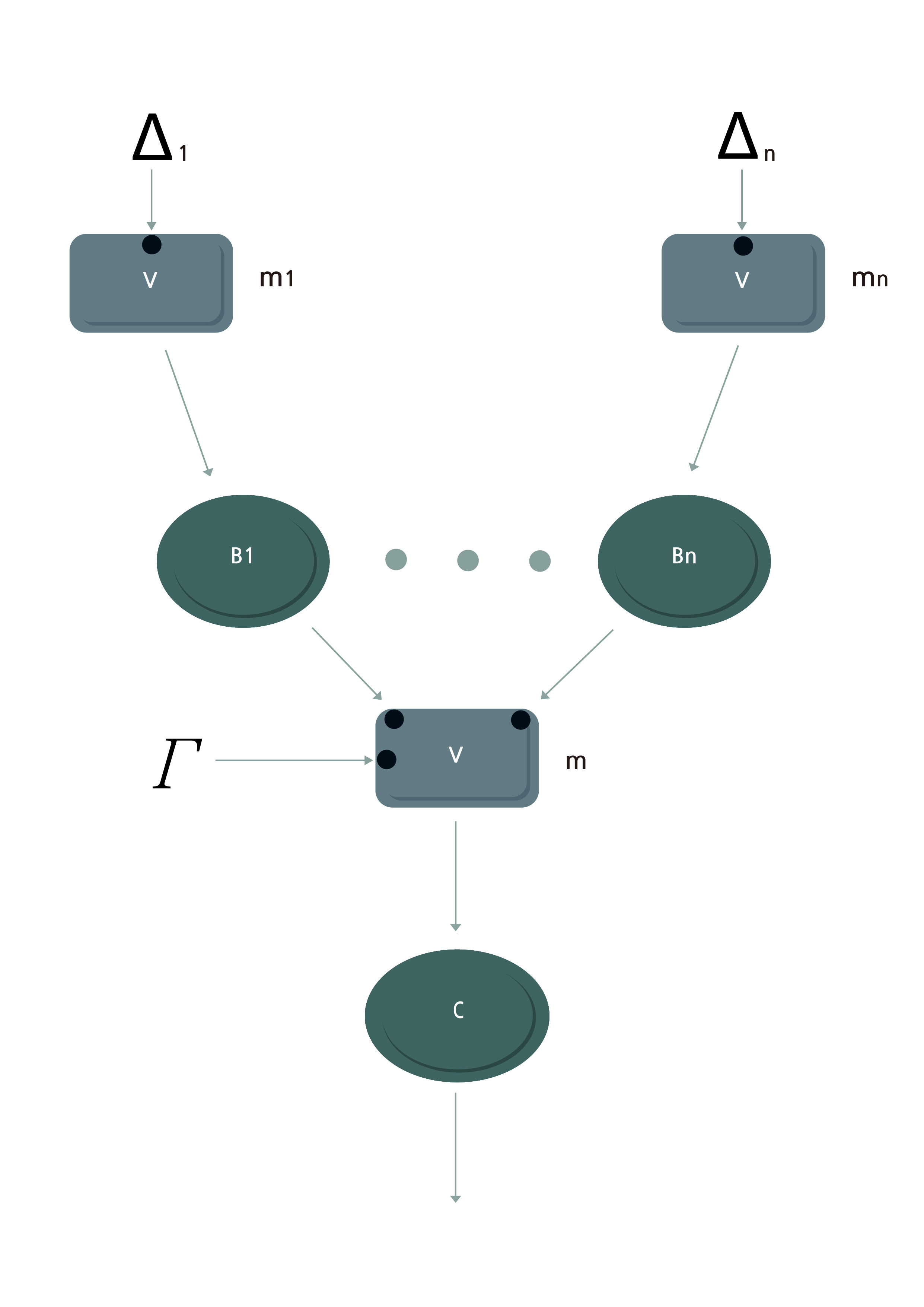
This MC’ rule leads to the diagram in Figure 1.

Figure 1: LFD for the multicut

In the diagram, note that each lemma $B_{i}$ is shared between $m_{i}$ and $m_{i+1}$. We call this diagram LFD with the following features:

• A regular arrow to box B with circle F means that some unknown identity (e.g. Nature) provides a regular service $F$ to B. Regular services include $sunny$ or $prime(2)$.

• A regular arrow from box A to box B with circle F in the middle means that A provides a querying service F to B.

• Knowledgebase(KB) of an agent is marked with $\bullet$s. In contrast, queries to the agent is marked without $\bullet$s.

• We assume that the top-level operator associated with an agent is  $\vee$ . That is, an agent with multiple KB services $KB_{1},\ldots,KB_{m}$ and a query services $Q$ should be understood as an agent with a query service $\mbox{\small$\neg$}KB_{1}\hskip 2.0pt\mbox{\small$\vee$}\hskip 2.0pt\ldots\hskip 2.0pt\mbox{\small$\vee$}\hskip 2.0pt\mbox{\small$\neg$}KB_{m}\hskip 2.0pt\mbox{\small$\vee$}\hskip 2.0ptQ$.

LFD can be seen as a modular alternative to the “flow proof” which is popular in mathematical education.

2 Examples

As an example of LFD, we will look at Peano Arithmetic (PA). PA is formulated with the usual $0,1,+,\times,=$. This is shown below.

$PA$ rules.

(1)$\mbox{$\forall$}x\mbox{$\forall$}y(x+1=y+1\hskip 2.0pt\mbox{\small$\rightarrow$}\hskip 2.0ptx=y)$.

(2)$\mbox{$\forall$}x(x+1\neq 0)$.

(3)$0+1=1$.

(4)$\mbox{$\forall$}x(x+0=x)$.

(5)$\mbox{$\forall$}x\mbox{$\forall$}y(x+(y+1)=(x+y)+1)$.

(6)$\mbox{$\forall$}x(x\times 0=0)$.

(7)$\mbox{$\forall$}x\mbox{$\forall$}y(x\times(y+1)=(x+y)+x)$.

(8)$\mbox{$\forall$}Q((Q(0)\hskip 2.0pt\mbox{\small$\wedge$}\hskip 2.0pt\mbox{$\forall$}x(Q(x)\hskip 2.0pt\mbox{\small$\rightarrow$}\hskip 2.0ptQ(x+1)))\hskip 2.0pt\mbox{\small$\rightarrow$}\hskip 2.0pt\mbox{$\forall$}xQ(x))$.

Rule (8) is called the Induction rule.

Figure 2: LFD for the example

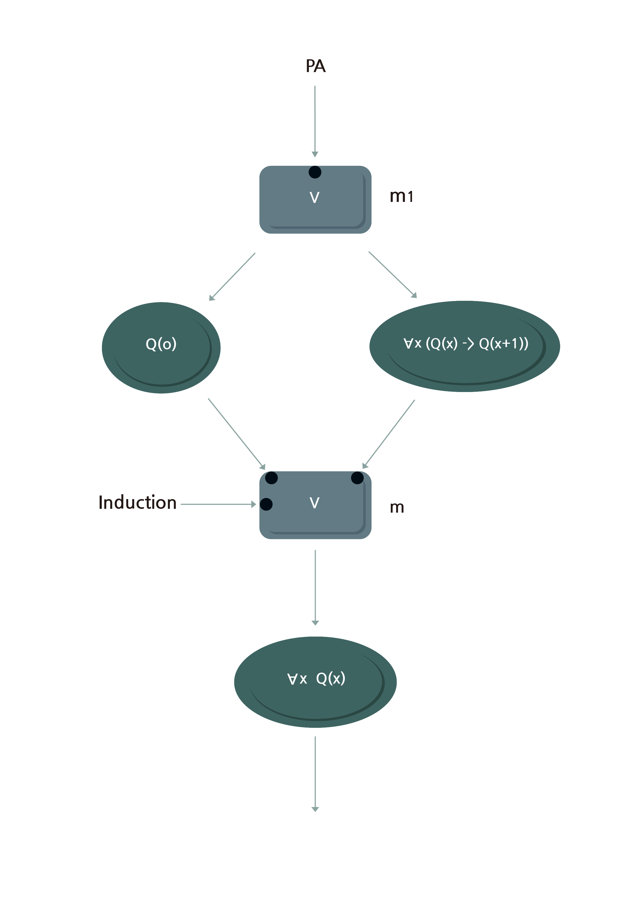
Now we want to prove the following:

$$\mbox{$\forall$}x(x+1=1+x)$$

The proof requires mathematical induction with $Q(x)$ being $(x+1=1+x)$. The base case $Q(0)$ which is $(0+1=1+0)$ follows from axiom 3 and 4. The induction step follows from induction hypothesis and axiom 5.

We display the LFD of the above example in Figure 2. This diagram is straightforward to understand.

3 Distributed first-order logic

To represent the ‘querying’ formulas in the MC’ rule, we need a new representation language, because they are not allowed in classical logic. For this reason, we introduce FOL^Ω which provides an elegant solution in this regard.

FOL^Ω is based on the game semantics. For this reason, we review the the game-semantical meanings of first-order logic[3].

First of all, classical propositions are viewed as special, elementary sorts of games that have no moves and are automatically won by the machine if true, and lost if false. For example, the proposition $prime(5)$ is true and is automatically won by the machine.

There are two special atoms $\top$ and $\bot$. $\top$ is always true, and $\bot$ is always false.

Negation $\neg$ is a role-switch operation: $\mbox{\small$\neg$}A$ is obtained from $A$ by turning $\top$’s moves and wins into $\bot$’s moves and wins, and vice versa. For example, if Chess means the game of chess from the view of the black player, then $\neg$Chess is the same game from the of view of the white player.

The parallel operations deal with concurrent computations. Playing $A\hskip 2.0pt\mbox{\small$\wedge$}\hskip 2.0ptB$ or $A\hskip 2.0pt\mbox{\small$\vee$}\hskip 2.0ptB$ means playing, in parallel, the two games $A$ and $B$. In $A\hskip 2.0pt\mbox{\small$\wedge$}\hskip 2.0ptB$, $\top$ is considered the winner if it wins in both of the components, while in $A\hskip 2.0pt\mbox{\small$\vee$}\hskip 2.0ptB$ it is sufficient to win in one of the components.

The reduction operation $A\hskip 2.0pt\mbox{\small$\rightarrow$}\hskip 2.0ptB$ is understood as $\mbox{\small$\neg$}A\hskip 2.0pt\mbox{\small$\vee$}\hskip 2.0ptB$.

The blind quantifiers $\mbox{$\forall$}xA$ and $\mbox{$\exists$}xA$ model information hiding with $\mbox{$\exists$}x$ meaning $\top$’s choices, and $\mbox{$\forall$}x$ meaning choices by $\bot$. In both cases, the value of $x$ is unknown or invisible to the opponent.

Following the ideas in [6], we introduce FOL^Ω, a slight extension to FOL with agent parameters. Let $F$ be a formula in first-order logic. We introduce a new env-annotated formula $F^{\omega}$ which reads as ‘play $F$ against an agent $\omega$. For $F^{\omega}$, we say $\omega$ is the matching environment of $F$.

In introducing agent parameters to a formula $F$, some formulas turn out to be difficult to process. ‘Environment-switching’ formulas are such examples. In them, the machine initially provides a service $F$ against agent $w$ and then switches to provide another service to another agent $u$ inside $F$. This kind of formulas are difficult to process. This leads to the following definition:

Definition 3.1.

The class of FOL^Ω-formulas is defined as the smallest set of expressions such that (a) For any FOL-formula $F$ and any agent $\omega$, $F^{\omega}$ is in it and, (b) if $H$ and $J$ are in it, then so are $\mbox{\small$\neg$}H,H\hskip 2.0pt\mbox{\small$\wedge$}\hskip 2.0ptJ,H\hskip 2.0pt\mbox{\small$\vee$}\hskip 2.0ptJ,H\hskip 2.0pt\mbox{\small$\rightarrow$}\hskip 2.0ptJ$.

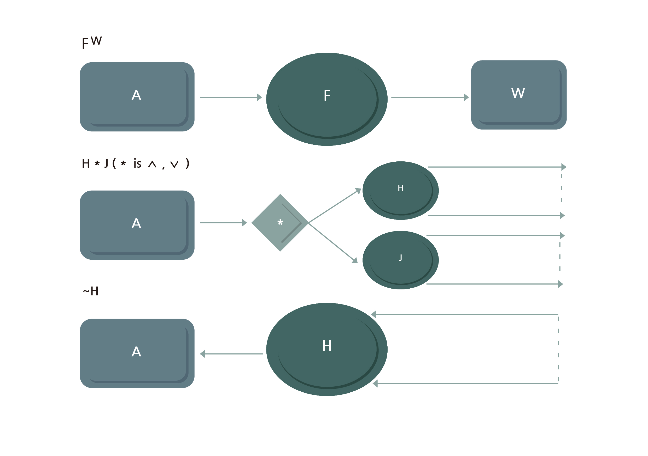
Given a FOL^Ω-formula $H$, the diagram of $H$ can be easily obtained.

Definition 3.2.

Given a FOL^Ω-formula $H$, the diagram of $H$ – denoted by $diagram(H)$ – is obtained by the rules in Figure 3. There, $F$ is a FOL-formula and $H,J$ are FOL^Ω-formulas. Further, $A$ is the current machine, $W$ is an environment.

Figure 3: FOL^Ω-formulas to diagrams

4 An Example: Encoding the Peano Axiom

The diagram in Section 2 corresponds to the following FOL^Ω. The (KB of) agent $m_{1}$ is shown below.

$agent\ m_{1}$.

$\mbox{$\forall$}x\mbox{$\forall$}y(x+1=y+1\hskip 2.0pt\mbox{\small$\rightarrow$}\hskip 2.0ptx=y)$.

$\mbox{$\forall$}x(x+1\neq 0)$.

$0+1=1$.

$\mbox{$\forall$}x(x+0=x)$.

$\mbox{$\forall$}x\mbox{$\forall$}y(x+(y+1)=(x+y)+1)$.

$\mbox{$\forall$}x(x\times 0=0)$.

$\mbox{$\forall$}x\mbox{$\forall$}y(x\times(y+1)=(x+y)+x)$.

Our language permits ‘querying knowledge’ of the form $Q^{\omega}$ in KB. This requires the current machine to invoke the query $Q$ to the agent $\omega$. Now let us consider the $m$ agent which handles mathematical induction. It contains the induction rule and two querying knowledges $Q(0)^{m_{1}}$ and $(\mbox{$\forall$}x(Q(x)\hskip 2.0pt\mbox{\small$\rightarrow$}\hskip 2.0ptQ(x+1)))^{m_{1}}$. Note that the induction rule is technically not first-order but it does not affect our main argument.

$agent\ m$.

$Q(0)^{m_{1}}$.

$(\mbox{$\forall$}x(Q(x)\hskip 2.0pt\mbox{\small$\rightarrow$}\hskip 2.0ptQ(x+1)))^{m_{1}}$.

$\mbox{$\forall$}Q((Q(0)\hskip 2.0pt\mbox{\small$\wedge$}\hskip 2.0pt\mbox{$\forall$}x(Q(x)\hskip 2.0pt\mbox{\small$\rightarrow$}\hskip 2.0ptQ(x+1)))\hskip 2.0pt\mbox{\small$\rightarrow$}\hskip 2.0pt\mbox{$\forall$}xQ(x))$.

Last, the theorem to prove corresponds to the query ?- $\mbox{$\forall$}x(x+1=1+x)$ with respect to the $m$ agent.

It can be easily observed that the above code can be automated. This leads to the notion of Lemma Flow Theorem Proving. Now, solving the above goal has the following strategy: first solve both the query $Q(0)^{m_{1}}$ and $(\mbox{$\forall$}x(Q(x)\hskip 2.0pt\mbox{\small$\rightarrow$}\hskip 2.0ptQ(x+1)))^{m_{1}}$ with respect to $m_{1}$ and then solve $\mbox{$\forall$}x(x+1=1+x)$ with respect to $m$. Note that all three attempts must succeed for $\mbox{$\forall$}x(x+1=1+x)$ to be true.

5 Conclusion

In this paper, we have considered a proof design tool called LFD and a distributed first-order logic FOL^Ω. Our diagram allows modular, distributed proof design. It is therefore useful for reading/writing/automating proofs. FOL^Ω has a simple syntax and semantics and is well-suited to representing distributed KB [7].

6 Acknowledgements

This work was supported by DongA University Research Fund.

References

- [1] Japaridze G. Introduction to computability logic. Annals of Pure and Applied Logic, 2003, 123(1/3): 1-99.
- [2] Japaridze G. Computability logic: a formal theory of interaction. In Interactive Computation: The New Paradigm, Goldin D, Smolka S A, Wegner P (eds.), Springer, 2006, pp. 183-223.
- [3] Japaridze G. In the beginning was game semantics. In Games: Unifying Logic, Language and Philosophy, Majer O, Pietarinen A -V, Tulenheimo T (eds.), Springer, 2009, pp. 249-350.
- [4] Japaridze G. Towards applied theories based on computability logic. Journal of Symbolic Logic, 2010, 75(2): 565-601.
- [5] Japaridze G. On the system CL12 of computability logic. http://arxiv.org/abs/1203.0103, June 2013.
- [6] Kwon K. Towards distributed logic programming based on computability logic. http://arxiv.org/abs/1909.07036, 2019.
- [7] S.W. Loke and A. Davison: LogicWeb: Enhancing the Web with Logic Programming. Journal of Logic Programming, 1998, 36(3): 195-240.