IMAGE DENOISING WITH LESS ARTEFACTS:
NOVEL NON-LINEAR FILTERING ON FAST PATCH REORDERINGS

Abstract

Leading denoising methods such as 3D block matching (BM3D) are patch-based. However, they can suffer from frequency domain artefacts and require to specify explicit noise models. We present a patch-based method that avoids these drawbacks. It combines a simple and fast patch reordering with a non-linear smoothing. The smoothing rewards both patch and pixel similarities in a multiplicative way. We perform experiments on real world images with additive white Gaussian noise (AWGN), and on electron microscopy data with a more general additive noise model. Our filter outperforms BM3D in 77% of the experiments, with improvements of up to 29% with respect to the mean squared error.

Index Terms—  non-local patch-based methods, diffusion methods, image denoising, additive white Gaussian noise

1 Introduction

Non-local patch-based methods [1, 2, 3, 4, 5, 6] have been producing superior image denoising results since quite a few years now. These models offer two main advantages: Firstly, the assumption that similar pixels have similar neighbourhoods around them, is quite robust in a noisy scenario. Secondly, one can access similar data from distant regions in the image.

The non-local Bayes (NLB) [7, 2] and BM3D [3, 8] approaches produce state-of-the-art results. NLB uses Bayesian modelling while BM3D employs Fourier domain filtering. However, it is well known that when the assumptions about noise-free images are violated, one can see artefacts in the denoised images. The idea that we can find completely similar patches within an image in general need not be satisfied. Thus, there is a risk that data from dissimilar regions can diffuse into each other, which leads to the above mentioned artefacts. This observation is well documented for both NLB and BM3D [6].

One remedy to eliminate these artefacts is to use an additional post-processing step [6]. Another possibility which was proposed by Ram et al. [4, 5] is to employ a smooth reordering of patches for subsequent filtering. However, the underlying reason why the latter method is better than BM3D is not well understood. It appears plausible to us that it minimises information exchange between dissimilar regions with the help of patch reordering, thus reducing the artefacts and consequently leading to better results. However, this comes at a computationally very expensive reordering step, which basically requires to solve a travelling salesman problem.

Our Contribution. We introduce a new method to solve the above artifact problem without the need of an additional post-processing step and also within a relatively low computational time. In contrast to the methods of Ram et al. [4, 5], we use a simpler and much faster patch reordering, and combine it with a more sophisticated non-linear filtering. Hence, we call our method non-linear filtering on fast patch reorderings (NFPR). In particular, we employ a filtering technique which is a novel combination of weights that reward both patch and pixel similarities. Moreover, we always use disc-shaped windows, thus leading to a rotationally invariant model. In contrast to NLB and BM3D, we avoid an explicit AWGN assumption and hence are more robust with respect to the noise type.

Paper Structure. In Section 2, we introduce our proposed NFPR framework for noise elimination along with proper motivations. In Section 3, we showcase a comparative evaluation of NFPR with NLB, BM3D and the method of Ram et al. [4], for both real-world test images and electron microscopy data. Finally, in Section 4, we conclude with a summary of our contribution and an outlook to future work.

Image	$\sigma$	$\lambda$	$k_{\textrm{max}}$	NFPR	NLB	BM3D
L40	150	11.5	16	74.00	69.30	68.27
L60	160	15.5	16	104.58	109.3	104.83
L80	175	20.0	14	139.37	154.40	143.23
L100	175	23.5	16	164.85	198.89	183.78
L120	190	27.0	15	196.96	254.90	228.39
L140	195	31.5	15	231.48	312.95	273.09
B40	130	15.0	13	254.87	233.36	233.34
B60	160	20.5	8	333.37	333.22	315.37
B80	165	26.0	9	400.71	425.61	391.02
B100	180	30.5	9	457.70	486.65	453.37
B120	180	34.5	10	505.86	551.94	512.38
B140	190	36.5	11	556.54	616.51	572.44
H40	140	10.5	27	58.77	62.16	56.01
H60	160	12.0	27	81.24	104.85	92.15
H80	180	15.0	23	116.63	156.88	130.64
H100	185	17.5	17	153.27	218.91	187.60
H120	205	22.5	17	192.11	289.12	235.53
H140	200	25.0	19	233.62	356.59	300.88
P40	155	11.5	16	57.73	60.03	58.91
P60	160	16.0	17	83.73	95.22	91.16
P80	185	18.5	15	112.39	128.95	124.08
P100	195	21.0	15	139.05	171.88	160.88
P120	205	25.0	15	167.70	216.02	200.58
P140	205	29.5	15	198.83	266.79	241.20

Table 1: MSE values of denoised images including NFPR parameters. L40 stands for Lena image with $\sigma_{\textrm{noise}}$ = 40. B, H, P denote Bridge, House and Peppers respectively.

2 Modelling of our denoising algorithm

Our NFPR technique consists of two parts: The goal of the first step is to achieve a fast patch-based reordering of the pixels. In the second step, we employ a non-linear smoothing on the reordered pixels which yields the denoised image. In the following we describe these steps in detail.

Step 1 : Fast Patch Reordering. In order to compute a smooth reordering of pixels, we employ a patch-based similarity approach: We first consider a disc-shaped search region $B_{\textrm{search}}$ of radius $\rho_{\textrm{search}}$ around every pixel $u_{i}$ in the 2D image domain. We then compute the $L_{2}$ norm $d_{ij}$ between disc-shaped patches of radius $\rho_{\textrm{sim}}$, centered around $u_{i}$ and $u_{j},$ for all $j\in B_{\textrm{search}}$. This is followed by constructing a set $P_{i}$ of $N$ pixels within $B_{\textrm{search}}$ which have the least distance from $u_{i}$ according to $d_{ij}$. This set characterises the desired smooth reordering of pixels. In contrast to Ram et al. [4, 5] who solve instances of the NP-hard travelling salesman problem, we compute the reordering using just a simple sort operation. Ideally, when we average noisy versions of the same greyvalue, we should not introduce artefacts. However, we have noisy versions of approximately equal grey values in the set $P_{i}$. Moreover, the above simple reordering is achieved at the cost of some disordered pixels in $P_{i}$, that come from areas of dissimilar greyvalues. In the second step of the algorithm, we employ a very robust non-linear smoothing technique, to deal with both problems.

Step 2 : Non-linear Smoothing. The goal of this step is to optimally combine the set of pixels $P_{i}$, obtained from the first step, and compute a final denoised image. To this end, we apply a non-linear smoothing process on this set. This can be thought of as diffusing information between pixels in a space defined by the neighbourhood similarity distances $d_{ij}$ instead of the generally used spatial distances. We utilise two assumptions which form the core of our structure preserving smoothing technique: Firstly, similar pixels have relatively smaller absolute tonal differences $|u_{j}-u_{i}|$. Secondly, they also have similar neighbourhoods around them. Although we have already used such an idea for patch reordering, we will be re-using the distances $d_{ij}$ through a multiplicative combination of both assumptions. This gives us an advantage in scenarios where one of the assumptions might be violated in the presence of noise. The discrete evolution equation for our smoothing process is given by

$$\frac{u_{i}^{k+1}-u_{i}^{k}}{\tau}=a_{i}^{k}\cdot\left(\sum_{\begin{subarray}{c}j\in P_{i}^{k}\end{subarray}}g\left({u^{k}_{\sigma j}}-{u^{k}_{\sigma i}}\right)h\left(d_{ij}^{k}\right)\left(u_{j}^{k}-u_{i}^{k}\right)\right.$$

$$+\left.\sum_{\begin{subarray}{c}j\in P^{\textrm{add},k}_{i}\end{subarray}}g\left({u^{k}_{\sigma j}}-{u^{k}_{\sigma i}}\right)h\left(d_{ij}^{k}\right)\left(u_{j}^{k}-u_{i}^{k}\right)\right).$$ (1)

This equation has two terms on the right hand side, which model two types of information exchange: Remember that $P_{i}$ denotes the set of pixels which are closest to pixel $u_{i}$ according to the distance $d_{ij}$. Every pixel in the image will have its own reordered set. Thus, the pixel $u_{i}$ could also be part of sets other than $P_{i}$. The symbol $P^{\textrm{add}}_{i}$ denotes an additional set of pixels in whose corresponding reordered sets, $u_{i}$ is present. The two terms mentioned in the above equation represent interactions with these two sets of pixels $P_{i}$ and $P^{\textrm{add}}_{i}$, respectively. This can also be seen as collaborative filtering similar to BM3D and NLB.

Image	$\sigma$	$\lambda$	$k_{\textrm{max}}$	NFPR	REC
L50	150	14.5	17	91.36	82.90
L75	170	19.0	15	126.90	123.75
L100	175	23.5	16	164.85	163.05
H50	160	11.0	23	70.94	74.45
H75	165	15.5	23	108.71	120.41
H100	185	17.5	17	153.27	167.52

Table 2: MSE values of denoised images including NFPR parameters. Abbreviations as in Table 1, REC - Ram et al. [4].

noisy                 NLB                 BM3D                 NFPR               original
                               

Fig. 1: Top to Bottom: Zoom into Lena, Bridge, House and Peppers images ($\sigma_{\mathrm{noise}}=80$).

noisy                         NFPR                                        FRC plot
                 

Fig. 2: Left: Zoom into ribosome image of a yeast cell, with original size 256 $\times$ 256. Right: Zoom into the [0.4-1.0] correlation range of the corresponding FRC plot calculated for 64 frequency levels. NFPR parameters used:- $\sigma=170,\lambda=2.5,k_{\textrm{max}}=35$. For NLB and BM3D we have optimised the unknown $\sigma_{\textrm{noise}}$ with respect to FRC.

Let us now discuss the details of the above two individual terms: The functions $g$ and $h$ model the above mentioned tonal and neighbourhood similarity assumptions, respectively. However, if we look closely at the argument of $g$, we have ${u_{\sigma j}}-{u_{\sigma i}}$ instead of ${u_{j}}-{u_{i}}$ which are the real tonal differences. This idea of calculating the tonal differences on a denoised image $\bm{u}_{\sigma}$, for a robust performance, is inspired from diffusion-based methods [9]. We have chosen a collaborative version of the non-local means approach [1] for this initial denoising process:

$$u^{k}_{\sigma i}=b_{i}^{k}\cdot\left(\sum_{\begin{subarray}{c}j\in P_{i}^{k}\end{subarray}}h\left(d_{ij}^{k}\right)u_{j}^{k}+\sum_{\begin{subarray}{c}j\in P^{\textrm{add},k}_{i}\end{subarray}}h\left(d_{ij}^{k}\right)u_{j}^{k}\right).$$ (2)

The symbols $a_{i}$ and $b_{i}$ in (2) and (2), respectively, are the normalisation constants. The functions $g$ [10] and $h$ in (2) are chosen as

$$g\left(s\right)=1-\text{exp}\left(\frac{-3.31488}{\left(\frac{s}{\lambda}\right)^{8}}\right),$$

$$h(s)=\text{exp}\left(\frac{-s^{2}}{2\sigma^{2}}\right).$$

The time step size $\tau$ in (2) is selected such that the maximum-minimum principle is not violated. This means that the dynamic range of the denoised image does not exceed that of the initial noisy image. We can achieve this by choosing $a_{i}$ = $b_{i}/M_{i}$, where $M_{i}$ is the sum of number of elements in $P_{i}$ and $P_{i}^{\textrm{add}}$, and $\tau\leq 1$. Finally, we iterate NFPR for $k_{\textrm{max}}$ times. We initialise the non-linear smoothing with the initial noisy image $\bm{f}$ and the patch reordering using a Gaussian smoothed version of $\bm{f}$ with standard deviation $\sigma_{G}$.

3 Experiments and Discussion

In order to test the robustness of our method with respect to the noise type, we have performed denoising experiments on both real-world test images and electron microscopy data. For saving time, we have restricted the usage of our patch reordering step to just two iterations. This has negligible effect on the denoising output. We have fixed the following parameters: $\rho_{\textrm{search}}=10$, $\rho_{\textrm{sim}}=10$, $\sigma_{G}=2.5$, $\tau=0.95$ and the number of elements in the reordered set $N=35$. In order to have a correspondence for the parameter $\sigma$ between real-world and electron microscopy data, we have performed an affine rescaling of the distances $d_{ij}$ within the set $P_{i}$, to [0, 255]. Thus, we just optimise the parameters $\sigma$, $\lambda$ and $k_{\textrm{max}}$. As already mentioned, our denoising experiments employ NLB, BM3D, Ram et al. [4] for comparison purposes with available implementations and detailed parameter studies in [7, 8, 11, 4].

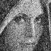
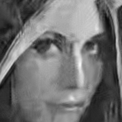
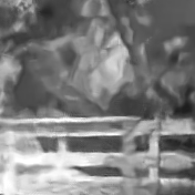
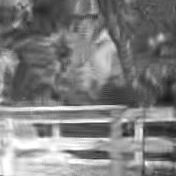
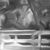
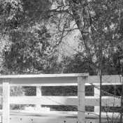
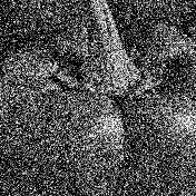
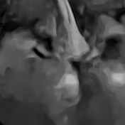
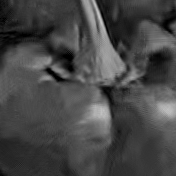
We first present our results on the real-world images Lena, Bridge, House and Peppers, which have been corrupted with AWGN. We use the mean squared error (MSE) for both measuring the quality of the denoised images and optimising the parameters. Figure 1 and Table 1 show the comparison with NLB and BM3D. Visual advantages in terms of less artefacts and more pleasant edges are larger than MSE advantages would suggest. From Table 2, we can conclude that our method is competetive with the approach of Ram et al. [4].

Experiments on a GPU show that our method takes just 2 and 6.5 seconds for denoising the $256\times 256$ sized House and $512\times 512$ sized Lena images ($\sigma_{\textrm{noise}}=100$), respectively. This implementation could further be improved with pre-computing the weighting functions and also through faster implementations of patch-similarity computations. The available non-parallel CPU implementation of [4] takes 1128 and 7021 seconds in the above scenarios. This is very expensive, even if we take into account the technical differences in the implementations.

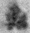
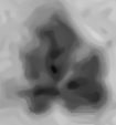
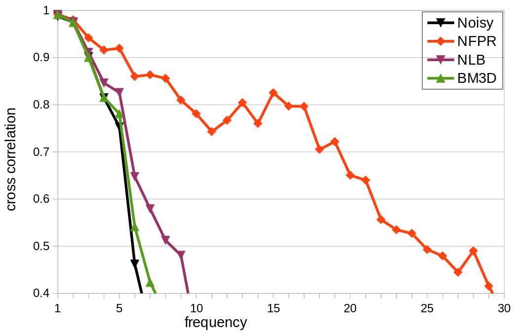
We have also considered ribosomal data in yeast cells acquired using an electron microscope. For measuring the quality of the denoised images, we use a popular frequency domain measure in electron microscopy called Fourier ring correlation (FRC). It computes a cross-correlation coefficient between the denoised versions of two different images of the same scene at different frequency levels [12, 13]. Figure 2 shows the corresponding results. We observe higher correlation coefficients for NFPR in the FRC curves. This indicates that it does a better job in preserving image structures during the denoising process.

All the above results can be attributed to the previously mentioned modelling advantages of NFPR. In contrast to NLB and BM3D, it also benefits by avoiding an explicit AWGN noise approach. This leads to even better NFPR results for electron microscopy data, as such kind of data is generally approximated with a more general additive noise model (see Chapter 11 of [14]). On the other hand, there are certainly some cases when NLB, BM3D and Ram et al. [4] are better than NFPR for real-world images like Lena and Bridge which have some amount of texture.

We observe that an important message from the above results is in accordance with the conclusion in our multi-frame denoising research [11]: The process of choosing the combination of pixels that undergo non-linear smoothing is as important as choosing the type of non-linearity itself. In BM3D and NLB, we filter a group of similar patches altogether. In NFPR, we utilise a carefully chosen set of pixels and subsequently filter them using a robust procedure. This is superior although we do not use any explicit spatial context in the filtering process. Unlike NLB and BM3D, we apply it only for patch reordering. In [11], we observed that a linear temporal filter can outperform a non-linear one, but only if the pixels that undergo the denoising process are chosen carefully.

4 Conclusions and Outlook

Although most people would agree that artifact avoidance is desirable in denoising, this goal has hardly been addressed in practice. It appears that smooth patch reordering is helpful in that aspect, but its computational workload is usually very high. The message of our paper is that this patch reordering can be fairly simplistic and therefore fast, provided that one comes up with more sophisticated non-linear filters that reward pixel and patch similarities in a multiplicative manner. Moreover, refraining from explicit noise models can be beneficial in real-world applications that may deviate from ideal noise assumptions. We believe that these are fairly general design principles that deserve further exploration in the future. This is also part of our ongoing work.

References

- [1] A. Buades, B. Coll, and J.-M. Morel, “A non-local algorithm for image denoising,” in Proc. IEEE Conference on Computer Vision and Pattern Recognition (CVPR), San Diego, CA, June 2005, vol. 2, pp. 60–65.
- [2] M. Lebrun, A. Buades, and J.M. Morel, “A nonlocal Bayesian image denoising algorithm,” SIAM Journal on Imaging Sciences, vol. 6, no. 3, pp. 1665–1688, Sept. 2013.
- [3] K. Dabov, A. Foi, V. Katkovnik, and K. Egiazarian, “Image denoising by sparse 3D transform-domain collaborative filtering,” IEEE Transactions on Image Processing, vol. 16, no. 8, pp. 2080–2095, Aug. 2007.
- [4] I. Ram, M. Elad, and I. Cohen, “Image processing using smooth ordering of its patches,” IEEE Transactions on Image Processing, vol. 22, no. 7, pp. 2764–2774, July 2013.
- [5] I. Ram, M. Elad, and I. Cohen, “Image denoising using NL-means via smooth patch ordering,” in Proc. IEEE International Conference on Acoustics, Speech and Signal Processing (ICASSP), Vancouver, BC, Canada, May 2013, pp. 1350–1354.
- [6] N. Pierazzo, M. E. Rais, J. M. Morel, and G. Facciolo, “DA3D: Fast and data adaptive dual domain denoising,” in Proc. IEEE International Conference on Image Processing (ICIP), Quebec City, Canada, Sept. 2015, pp. 432–436.
- [7] M. Lebrun, A. Buades, and J.M. Morel, “Implementation of the Non-Local Bayes (NL-Bayes) image denoising algorithm,” Image Processing On Line, vol. 3, pp. 1–42, June 2013.
- [8] M. Lebrun, “An analysis and implementation of the BM3D image denoising method,” Image Processing On Line, vol. 2, pp. 175–213, Aug. 2012.
- [9] F. Catté, P.-L. Lions, J.-M. Morel, and T. Coll, “Image selective smoothing and edge detection by nonlinear diffusion,” SIAM Journal on Numerical Analysis, vol. 29, no. 1, pp. 182–193, Mar. 1991.
- [10] J. Weickert, Anisotropic Diffusion in Image Processing, Teubner, Stuttgart, 1998.
- [11] K. Bodduna and J. Weickert, “Removing Multi-frame Gaussian Noise by Combining Patch-based Filters with Optical Flow,” arXiv:2001.08058 [eess.IV], Jan. 2020.
- [12] W. O. Saxton and W. Baumeister, “The correlation averaging of a regularly arranged bacterial cell envelope protein,” Journal of Microscopy, vol. 127, no. 2, pp. 127–138, Aug. 1982.
- [13] P. A. Penczek, “Resolution measures in molecular electron microscopy,” Methods in Enzymology, vol. 482, pp. 73–100, 2010.
- [14] J. Frank, Electron Tomography: Methods for Three-dimensional Visualisation for Structures in the Cell, Springer, New York, second edition, 2008.