Info-Commit: Information-Theoretic
Polynomial Commitment

Abstract

We introduce Info-Commit, an information-theoretic protocol for polynomial commitment and verification. With the help of a trusted initializer, a succinct commitment to a private polynomial $f$ is provided to the user. The user then queries the server to obtain evaluations of $f$ at several inputs chosen by the user. The server provides the evaluations along with proofs of correctness which the user can verify against the initial commitment. Info-Commit has four main features. Firstly, the user is able to detect, with high probability, if the server has responded with evaluations of the same polynomial initially committed to. Secondly, Info-Commit provides rigorous privacy guarantees for the server: upon observing the initial commitment and the response provided by the server to $m$ evaluation queries, the user only learns $O(m^{2})$ symbols about the coefficients of $f$. Thirdly, the verifiability and the privacy guarantees are unconditional regardless of the computational power of the two parties. Lastly, Info-Commit is doubly-efficient in the sense that in the evaluation phase, the user runs in $O(\sqrt{d})$ time and the server runs in $O(d)$ time, where $d-1$ is the degree of the polynomial $f$.

I Introduction

Consider a user who wishes to delegate the task of running a proprietary software, such as an advanced optimization or a machine learning algorithm, on his data to an untrusted server. To enhance the credibility of the results, the server sends a proof of correctness along with the outcome of the computation to the user. On the other hand, the user may not be authorized to access the underlying software. Therefore, while the proof must be informative enough to convince the user of the correctness of the result, it should reveal as little information as possible about the underlying program. To enable this process, one could envision a trusted party who provides the user with a verification key. This party could be, for instance, the developer of the software. While the server may be incentivized to satisfy the customers with as little computational resources as possible, the developer has little reason to provide the users with a false verification key.

The literature on verifiable computing [1, 2, 3, 4] and functional commitment protocols [5, 6] allow the server (prover) to generate a proof of correctness of the results which can be efficiently checked by the users (verifiers). Such an algorithm is said to have the soundness property, if a malicious prover cannot provide a convincing proof of an incorrect evaluation to the verifier. In general, the soundness of these algorithms relies on heuristic hardness assumptions. Our goal in this paper is to design a commitment and verification algorithm that overcomes this limitation. Namely, (i) the verifiability property must hold regardless of the computation power of the prover, and (ii) the verifier must not learn more than a constant number of bits about the underlying function, regardless of the verifier’s computational power. In the example above, the prover should be able to keep the program private from the verifier while at the same time providing him with verifiable results. This verification is performed against an initial commitment by the prover which contains almost no information about the program itself. Once the verifier receives the commitment to a specific function, the prover will only be able to pass the verification process by providing evaluations of the same function that the prover has committed to. Our focus in this work is on functions that can be represented as polynomials. This encompasses a wide range of applications including transaction verification in cryptocurrencies [7, 8, 9, 10], verifiable secret sharing [11, 6], and proof-of-storage [12, 13, 4].

I-A Our contributions

We propose Info-Commit, an information-theoretic protocol for polynomial commitment and verification. Info-Commit consists of a commitment phase and an evaluation phase. In the commitment phase, a third-party initializer enables the verifier to learn a private commitment to the prover’s private polynomial $f$ of degree $d-1$ over a finite field $\mathbb{F}_{q}$. In the evaluation phase, the verifier requests evaluations of the polynomial $f$ at many input points from the prover. Info-Commit is verifiable, privacy-preserving and doubly-efficient. More specifically, Info-Commit has the following salient features.

1. Verifiability. If the prover commits to a polynomial $f$ in the commitment phase, the prover must provide evaluations of the same polynomial $f$ in the evaluation phase. Otherwise, the verifier can detect the inconsistency with high probability. On the other hand, if the prover is honest, the verifier accepts the results with probability $1$.

   Moreover, Info-Commit is adaptive as it remains secure even when the prover is informed about the verification outcome of the previous queries.

2. Privacy. The other facet of Info-Commit is its privacy-preserving property. Upon observing the initial commitment and the response of the prover to $m$ rounds of evaluation, the verifier only learns $O(m^{2})$ symbols over the finite field about the coefficients of the polynomial $f$.

3. Information-theoretic guarantees. Both the verifiability and the privacy guarantees of Info-Commit are information-theoretic, meaning that the verifier and the prover can have unbounded computational power and may arbitrarily deviate from the prescribed protocol.

4. Double-efficiency. For each evaluation round, the verifier runs in $O(\sqrt{d})$ time, whereas the prover runs in $O(d)$ time. Note that we measure the efficiency of Info-Commit in the amortized model [2], where the initial commitment phase is followed by many rounds of evaluations and the one-time cost of the commitment phase can be neglected.

I-B Related work

The closest works in the literature to this work are commitment protocols, including polynomial commitment [6, 14, 15, 16], vector commitment [17], cryptographic accumulators [18], and more generally functional commitments [5]. These protocols allow a prover to provide a cryptographic commitment to a specific function which reveals little to no information about the underlying function. A verifier can then request the prover to “open" the commitment at specific locations. The verifier should be able to detect if the opening is inconsistent with the initial commitment.
There are several factors that distinguish the model in the current paper from the traditional notion of functional commitment. The first difference is in the notion of privacy. The linear commitment model in [5] requires the initial commitment to reveal no information about the function. However, it does not impose any requirement on how much information is revealed upon observing the evaluations (opening) of the functions along with the initial commitment. On the other hand, the polynomial commitment scheme in [6] only requires the evaluations of the polynomial at unqueried points to remain hidden from the verifier, which is a rather weaker privacy constraint. In contrast, we impose rigorous information-theoretic constraints on how much information is revealed about the coefficients of the polynomial upon observing the initial commitment and the evaluations at a constant number of input points. Secondly, while the literature on functional commitment is more concerned with the size of the commitment and the size of the opening, we instead focus on designing doubly-efficient algorithms, i.e., algorithms with efficient provers and super-efficient verifiers. Furthermore, unlike the literature on functional commitment, our verifiability guarantee is information-theoretic.

Another relevant concept is zero-knowledge verifiable computation [19] and zero-knowledge arguments of knowledge [20, 21, 22, 23]. Such algorithms enable a verifier and a prover to interact to compute $f(v,u)$, where $f$ is a publicly known function, $v$ is the input of the verifier and $u$ is the private input of the prover. The verifier will not learn anything about $u$ except for what is implied through $f(v,u)$. Furthermore, the verifier will be convinced that there exists some $u$ known to the prover such that the computed value corresponds to $f(v,u)$. In the context of polynomial evaluation, $v$ could be the input to the polynomial, $u$ the coefficients of the polynomial, and $f$ an operator that maps $(v,u)$ to the evaluation of the polynomial. Unfortunately, this approach does not provide any binding guarantees, as the prover may change the polynomial for every input.

Other related notions in the literature are oblivious polynomial evaluation [24, 25, 26, 27] which guarantees the privacy of both parties in a semi-honest setting, and verifiable computation [2, 4, 28, 29] which guarantees efficient verifiability, but generally ignores the privacy of the prover. Info-Commit, however, jointly ensures privacy of the prover and efficient verifiability.

I-C Relation with INTERPOL [28]

INTERPOL was presented in [28] as an information-theoretic alternative to the existing cryptographic solutions for verifiable polynomial evaluation. In that context, both the verifier and the prover had access to the underlying polynomial. Info-Commit, on the other hand, is focused on the notion of polynomial commitment. The new challenge is to keep the underlying polynomial hidden from the verifier, while convincing the verifier that the results conform with an initial commitment. The evolution from INTERPOL to the present work has been outlined in Section III. Section III-A can be seen as a variation of INTERPOL which relies on a trusted initializer to eliminate the need for the verifier to access the entire polynomial. Section III-B enables privacy against a semi-honest verifier. Finally, Section III-C illustrates how to achieve privacy against a malicious verifier.

Organization. The rest of this paper is organized as follows. We provide a brief background and formally present the problem statement in Section II. An overview of Info-Commit is provided in Section III and then Section IV describes Info-Commit in detail. In Section V, we analyze the correctness, the complexity, the soundness and the privacy guarantees of Info-Commit. Finally, in Section VI, we discuss some concluding remarks.

II Preliminaries and Problem Statement

In this section, we provide a brief background and describe the polynomial commitment and verification problem.

II-A Preliminaries

The following definition and property will be useful in the analysis of Info-Commit.

Definition 1 (Markov Chain).

An ordered set of three random variables $(X,Y,Z)\in{\cal X}\times{\cal Y}\times{\cal Z}$ is said to form a Markov chain if

$$\mathbb{P}(X=x,Z=z|Y=y)=\mathbb{P}(X=x|Y=y)\mathbb{P}(Z=z|Y=y)$$ (1)

for every $(x,y,z)\in{\cal X}\times{\cal Y}\times{\cal Z}$. Intuitively, this means that the two random variables $X$ and $Z$ are independent, conditioned on knowing $Y$. This Markov chain is represented by $X\longleftrightarrow Y\longleftrightarrow Z$.

Property 1. If $X\longleftrightarrow Y\longleftrightarrow Z$ forms a Markov chain, then $H_{q}(X|Y,Z)=H_{q}(X|Y)$, where $H_{q}$ represents the Shannon entropy in base $q$.

II-B Polynomial commitment and verification

Suppose a prover is in possession of a private polynomial $f(x)=a_{0}+a_{1}x+\cdots+a_{d-1}x^{d-1}$ selected uniformly at random among all polynomials of degree $d-1$ over $\mathbb{F}_{q}$. A verifier, who only knows the degree of the polynomial, wishes to obtain evaluations of this polynomial at several input points $x\in\mathbb{F}_{q}$ and verify the correctness of the results in sub-linear time in $d$. Before this evaluation phase, the prover commits to the polynomial $f$ during an initialization phase. Once this commitment is done, the prover is expected to evaluate the same polynomial $f$ for every input $x\in\mathbb{F}_{q}$ provided by the verifier. The verifier should be able to detect, efficiently and with high probability, if for any input $x\in\mathbb{F}_{q}$ the prover returns an incorrect evaluation $y\neq f(x)$. We assume that the verifier is interested in evaluating the polynomial $f$ at many input points, so that the complexity of the commitment phase amortizes over many rounds of the evaluation phase [2]. Therefore, efficiency is only measured with respect to the evaluation phase. Additionally, during the entire commitment and evaluation phases, the verifier should only learn a negligible amount of information about the coefficients of the polynomial $f$. Note that revealing a constant number of symbols over $\mathbb{F}_{q}$ about the coefficients of $f$ to the verifier is inevitable, since such amounts of information can be learned by investigating a single pair $(x,f(x))$. Formally, a polynomial commitment and verification protocol consists of the following algorithms.

• Commit$(a_{0},\cdots,a_{d-1},K_{v},K_{p})$. In the commitment phase, the verifier and the prover engage in a commitment protocol Commit$(a_{0},\cdots,a_{d-1},K_{v},K_{p})$ to help the verifier learn a secret verification key VK which depends on the verifier’s secret key, $K_{v}$, the prover’s secret key, $K_{p}$, and the polynomial coefficients $a_{0},\cdots,a_{d-1}$.

• Eval$(x,a_{0},\cdots,a_{d-1},K_{p})$. The verifier requests an evaluation of $f$ at $x$ from the prover. The prover then provides $val=$Eval$(x,a_{0},\cdots,a_{d-1},K_{p})$ to help the verifier evaluate $f(x)$.

• Verify$(x,val,\text{VK},K_{v})$. The verifier checks the correctness of $val$ based on $K_{v}$ and VK. If $val$ is incompatible with the initial commitment, the verifier rejects the evaluation. Otherwise, the verifier proceeds to recover $f(x)$.

• Recovery$(x,val)$. If the verification process passes, the verifier will proceed to recover the evaluation $f(x)$ via an algorithm Recovery$(x,val)$.

We are interested in polynomial commitment and verification protocols that are information-theoretically private and efficiently verifiable as defined next.

Definition 2 (Information-theoretically Private and Verifiable Polynomial Commitment).

A polynomial commitment and verification protocol is information-theoretically private and verifiable if it satisfies the following properties.

• Correctness. If the prover follows the Commit and the Eval algorithms for the same polynomial $f$, then the Verify algorithm must return $1$ with probability $1$.

• (Information-theoretic) Soundness. If the prover commits to a polynomial with coefficients $a_{0},\cdots,a_{d-1}$, then the probability that the prover can pass the verification test with $\hat{val}\neq\text{\bf Eval}(x,a_{0},\cdots,a_{d-1},K_{p})$ should be negligible, regardless of the prover’s computational power. That is, we must have

  $$\Pr( \text{\bf Verify}(x,\hat{val},\text{VK},K_{v},K_{p})=1,$$

  $$\hat{val}\neq\text{\bf Eval}(x,a_{0},\cdots,a_{d-1},K_{p}))=o(1),$$ (2)

  where the term $o(1)$ vanishes as the finite field size $q$ grows.

• Efficient Verification. The two functions Verify and Recovery must run in sub-linear time in $d$.

• Efficient Evaluation. The running time of Eval must be comparable to the time required for evaluating the polynomial $f$, i.e., linear in $d$.

• (Information-theoretic) Privacy. After running Commit and Eval for $m$ different inputs $x_{1},\cdots,x_{m}$, the verifier should only learn $\rho=O(\mathrm{poly}(m))$ symbols over the field about the coefficients of the polynomial $f$, regardless of the verifier’s computation power. Importantly, $\rho$ should be independent of the degree of the polynomial. That is, we must have

  $$H_{q}(a_{0},\cdots,a_{d-1}|\text{VK},(x_{1},val_{1}),\cdots,(x_{m},val_{m}))$$

  $$=d-O(\mathrm{poly}(m)).$$ (3)

III An Overview of Info-Commit

In this section, we provide an overview of Info-Commit . We first note that the polynomial $f(x)=a_{0}+a_{1}x+\cdots+a_{d-1}x^{d-1}$ can be expressed as follows

$$f(x)=\begin{bmatrix}1&x^{s}&\cdots&x^{s(s-1)}\end{bmatrix}\mathbfsl A\begin{bmatrix}1&x&\cdots&x^{s-1}\end{bmatrix}^{\mathrm{T}},$$ (4)

where $s=\sqrt{d}$, and

$$\mathbfsl A=\begin{bmatrix}a_{0}&a_{1}&\cdots&a_{s-1}\\ a_{s}&a_{s+1}&\cdots&a_{2s-1}\\ &\ddots&&\\ a_{s^{2}-s}&a_{s^{2}-s+1}&\cdots&a_{s^{2}-1}\end{bmatrix}.$$ (5)

III-A A basic algorithm

A straightforward algorithm is for the verifier to generate a $c\times s$ matrix $\mathbfsl\Lambda\in\mathbb{F}_{q}^{c\times s}$ uniformly at random, for some security parameter $c$. In the commitment phase, the verifier and the prover will engage in a commitment protocol through the trusted initializer to help the verifier learn

$$\mathbfsl\Gamma=\mathbfsl\Lambda\mathbfsl A.$$ (6)

In this process, the verifier will not learn anything about $\mathbfsl A$ other than what is revealed through $\mathbfsl\Gamma$, and the prover will not learn anything about $\mathbfsl\Lambda$. For instance, the verifier and the prover respectively provide $\mathbfsl\Lambda$ and $\mathbfsl A$ to the trusted party, and the trusted party sends $\mathbfsl\Gamma$ to the verifier. In the evaluation phase, the verifier will ask the prover to compute

$$\mathbfsl b=\mathbfsl A\begin{bmatrix}1&x&\cdots&x^{s-1}\end{bmatrix}^{\mathrm{T}}.$$ (7)

Suppose the prover responds with $\hat{\mathbfsl b}$. The verifier checks if

$$\mathbfsl\Lambda\hat{\mathbfsl b}=\mathbfsl\Gamma\begin{bmatrix}1&x&\cdots&x^{s-1}\end{bmatrix}^{\mathrm{T}},$$ (8)

which can be done in $O(\sqrt{d})$ time. If $\hat{\mathbfsl b}\neq\mathbfsl b$, this identity holds only with probability $q^{-c}$ [28], since the prover does not know anything about $\mathbfsl\Lambda$. If the verification process is successful, the verifier can recover

$$\hat{f}(x)=\begin{bmatrix}1&x^{s}&\cdots&x^{s(s-1)}\end{bmatrix}\hat{\mathbfsl b}$$ (9)

in $O(\sqrt{d})$ time and accepts it as the correct evaluation. This algorithm has been previously explored in [28].
The main issue with this algorithm is that $\mathbfsl\Gamma$ reveals $O(\sqrt{d})$ symbols over $\mathbb{F}_{q}$ about the polynomial $f$ during the commitment phase, and another $\sqrt{d}$ symbols for each evaluation $\mathbfsl b$. We wish to reduce this to a constant. We will accomplish this in two steps: firstly, against a semi-honest verifier in Section III-B and next against a malicious verifier in Section III-C.

III-B Improved privacy against a semi-honest verifier

In order to improve the privacy of this basic algorithm, the prover will generate a polynomial $g$ of degree $d-1$ uniformly among all polynomials of degree $d-1$ over $\mathbb{F}_{q}$. In the commitment phase, instead of directly committing to $f$, the prover commits to both $h=f+g$ and $g$. Let $\mathbfsl A$ and $\mathbfsl B$ represent the $s\times s$ matrices corresponding to the polynomials $f$ and $g$, constructed similarly to (5). If both commitments have the same structure as in (6), the verifier will be able to gain substantial information about the matrix $\mathbfsl A$ by choosing the two secret matrices to be linearly dependent.

To prevent this, the protocol will require the prover to commit to $\mathbfsl A+\mathbfsl B$ “from the left" as in (6), whereas the commitment to $\mathbfsl B$ will be done “from the right". More concretely, the verifier and the prover engage in commitment algorithm through the trusted initializer such that the verifier learns

$$\mathbfsl\Gamma =\mathbfsl\Lambda(\mathbfsl A+\mathbfsl B),$$

$$\mathbfsl\Omega =\mathbfsl B\mathbfsl\Theta^{\mathrm{T}},$$ (10)

for two $c\times s$ secret matrices $\mathbfsl\Lambda$ and $\mathbfsl\Theta$ generated uniformly at random by the verifier. To gain intuition on how this preserves the privacy of $\mathbfsl A$, it helps to consider the case of $c=1$. Knowing any single linear combination of the rows of $\mathbfsl A+\mathbfsl B$ and any single linear combination of the columns of $\mathbfsl B$ cannot reveal more than one symbol over $\mathbb{F}_{q}$ about the elements of the matrix $\mathbfsl A$. This argument will be made precise in the privacy analysis of Info-Commit in Section V. In the evaluation phase, the prover is asked to compute

$$\mathbfsl v =(\mathbfsl A+\mathbfsl B)\begin{bmatrix}1&x&\cdots&x^{s-1}\end{bmatrix}^{\mathrm{T}},$$

$$\mathbfsl u =\begin{bmatrix}1&x^{s}&\cdots&x^{s(s-1)}\end{bmatrix}\mathbfsl B.$$ (11)

Suppose the prover responds with $\hat{\mathbfsl v}$ and $\hat{\mathbfsl u}$. The verifier will check the correctness of each result via two parities

$$\mathbfsl\Gamma\begin{bmatrix}1&x&\cdots&x^{s-1}\end{bmatrix}^{\mathrm{T}} =\mathbfsl\Lambda\hat{\mathbfsl v},$$

$$\begin{bmatrix}1&x^{s}&\cdots&x^{s(s-1)}\end{bmatrix}\mathbfsl\Omega =\hat{\mathbfsl u}\mathbfsl\Theta^{\mathrm{T}}.$$ (12)

If both verification tests are successful, then the verifier recovers

$$\hat{h}(x) =\begin{bmatrix}1&x^{s}&\cdots&x^{s(s-1)}\end{bmatrix}\hat{\mathbfsl v},$$

$$\hat{g}(x) =\hat{\mathbfsl u}\begin{bmatrix}1&x&\cdots&x^{s-1}\end{bmatrix}^{\mathrm{T}}.$$ (13)

Finally, the verifier will find

$$\hat{f}(x)=\hat{h}(x)-\hat{g}(x)$$ (14)

and will accept $\hat{f}(x)$ as the correct evaluation of $f$ at $x$. This algorithm guarantees the verifiability of the results with high probability following a similar analysis to [28]. Nonetheless, the privacy only holds as long as $(\mathbfsl\Lambda,\mathbfsl\Theta)$ are generated uniformly at random over $\mathbb{F}_{q}^{c\times s}$, i.e., if the verifier is semi-honest. We will overcome this limitation in the next subsection.

III-C Improving privacy against a malicious verifier

If both parties follow the protocol of Section III-B as described, the verifier will only learn a constant number of symbols about the polynomial $f$ upon observing $(\mathbfsl\Gamma,\mathbfsl\Omega)$ and the pair $(\mathbfsl v,\mathbfsl u)$ for a constant number of inputs (see the analysis of privacy in Section V). However, a malicious verifier may deviate from this protocol by choosing $\mathbfsl\Lambda$ and $\mathbfsl\Theta$ in a deterministic manner as in the following example.

Example 1 (Malicious Verifier).

1. Commitment Phase. Suppose that $c=1$ and the verifier chooses $\mathbfsl\Lambda=\begin{bmatrix}1&0&\cdots&0\end{bmatrix}$. This helps the verifier learn $\mathbfsl\Gamma=\mathbfsl A_{1}+\mathbfsl B_{1}$, the first row of the matrix $\mathbfsl A+\mathbfsl B$.

2. Evaluation Phase. In this phase, the verifier requests the $(\mathbfsl v,\mathbfsl u)$ pair for $x=0$. Based on this, the verifier can learn $\mathbfsl u=\mathbfsl B_{1}$, which is the first row of the matrix $\mathbfsl B$.

3. The verifier then computes $\mathbfsl\Gamma-\mathbfsl u$ in order to find $\mathbfsl A_{1}$, which reveals $\sqrt{d}$ symbols about the polynomial $f$.

We will propose a mechanism to resolve this threat. Suppose the verifier requests the $(\mathbfsl v,\mathbfsl u)$ pair for $m$ different inputs $x_{1},\cdots,x_{m}$. Define the matrices $\mathbfsl X$ and $\mathbfsl Y$ as follows

$$\mathbfsl X =\begin{bmatrix}1&x_{1}&\cdots&x_{1}^{s-1}\\ &\cdots&\cdots&\\ 1&x_{m}&\cdots&x_{m}^{s-1}\end{bmatrix},$$

$$\mathbfsl Y =\begin{bmatrix}1&x_{1}^{s}&\cdots&x_{1}^{s(s-1)}\\ &\cdots&\cdots&\\ 1&x_{m}^{s}&\cdots&x_{m}^{s(s-1)}\end{bmatrix},$$ (15)

and let the matrices $\mathbfsl U$ and $\mathbfsl V$ be the concatenation of the vectors $\mathbfsl u$ and $\mathbfsl v$ for all $x\in\{x_{1},\cdots,x_{m}\}$ as follows

$$\mathbfsl V =(\mathbfsl A+\mathbfsl B)\mathbfsl X^{\mathrm{T}},$$

$$\mathbfsl U =\mathbfsl Y\mathbfsl B.$$ (16)

Since after $m$ rounds of evaluation, the verifier learns $\mathbfsl\Gamma=\mathbfsl\Lambda(\mathbfsl A+\mathbfsl B)$ and $\mathbfsl U=\mathbfsl Y\mathbfsl B$, the prover must ensure that the matrices $\mathbfsl\Lambda$ and $\mathbfsl Y$ do not contain any linear dependencies among their rows. Otherwise, this linear dependency can be exploited to extract substantial information about the matrix $\mathbfsl A$ as in Example 1. Since $\operatorname{rank}(\mathbfsl Y)=m$ and $\operatorname{rank}(\mathbfsl\Lambda)=c$ (with high probability), the prover must ensure that

$$\operatorname{rank}(\mathbfsl Y||\mathbfsl\Lambda)=c+m,$$ (17)

where $||$ denotes the vertical concatenation of the two matrices. Similarly, we must have

$$\operatorname{rank}(\mathbfsl X||\mathbfsl\Theta)=c+m.$$ (18)

To accomplish this, we restrict the matrices $\mathbfsl\Lambda$ and $\mathbfsl\Theta$ to have the same Vandermonde structures as the matrices $\mathbfsl Y$ and $\mathbfsl X$, respectively. In other words, $\mathbfsl\Lambda$ and $\mathbfsl\Theta$ must be of the form

$$\mathbfsl\Lambda =\begin{bmatrix}1&\lambda^{s}_{1}&\cdots&\lambda_{1}^{s(s-1)}\\ &\cdots&\cdots&\\ 1&\lambda^{s}_{c}&\cdots&\lambda_{c}^{s(s-1)}\end{bmatrix},$$

$$\mathbfsl\Theta =\begin{bmatrix}1&\theta_{1}&\cdots&\theta_{1}^{s-1}\\ &\cdots&\cdots&\\ 1&\theta_{c}&\cdots&\theta_{c}^{s-1}\end{bmatrix}.$$ (19)

Note that as long as

$$|\{\lambda_{1},\cdots,\lambda_{c},x_{1},\cdots,x_{m}\}| =|\{\theta_{1},\cdots,\theta_{c},x_{1},\cdots,x_{m}\}|$$

$$=c+m,$$ (20)

the two rank requirements will be satisfied. Note also that, without loss of generality, we can assume that $\lambda_{i}\neq\lambda_{j}$, $\theta_{i}\neq\theta_{j}$ and $x_{i}\neq x_{j}$ for $i\neq j$, since the verifier cannot benefit from receiving the same evaluation twice. Restricting the structure of $\mathbfsl\Lambda$ and $\mathbfsl\Theta$ as opposed to choosing them uniformly at random over $\mathbb{F}_{q}^{c\times s}$ would mean that the prover now has some side information about these matrices which can be utilized to bypass the verification test. Fortunately, the analysis in Section V shows that this probability remains sufficiently small.

It is left to convince the prover that (20) holds. For this purpose, we designate a set $S\subseteq\mathbb{F}_{q}$ of prohibited values from which the elements $\lambda_{i}$ and $\theta_{i}$ can be chosen. “Prohibited" means that in the evaluation phase, the verifier is not permitted to delegate the evaluation of the function $f$ at any member of $S$ to the prover. For instance, the verifier could provide an upper-bound $\xi$ on its input values to the prover, and then $S\subseteq\mathbb{F}_{q}$ could be chosen as a sufficiently large interval whose smallest member is strictly larger than $\xi$.

III-D Considerations regarding the size of the field

The privacy analysis of Info-Commit in Section V relies on the fact that the set $\{\alpha^{s}|\alpha\in S\}$ is of the same size as $S$, where $S$ is the set of prohibited values. This property holds if the function $g(x)=x^{s}$ is a permutation over $\mathbb{F}_{q}$ which is the case if $\mathrm{gcd}(s,q-1)=1$. It is also important that there exists a prohibited subset of $\mathbb{F}_{q}$ of sufficiently large size. To ensure this, either the verifier should set the upper bound $\xi$ appropriately, or the field size should be increased once the verifier provides the upper-bound. Of course, this adjustment must be done without violating the first property.

IV Formal Description of Info-Commit

The formal description of the four functions of Info-Commit, namely Commit, Eval, Verify and Recovery are provided in Algorithms 1,2,3 and 4, respectively. Theorem 1 establishes that Info-Commit satisfies the requirements of an information-theoretically verifiable and private protocol for commitment and verification.

1:Input: The private polynomial coefficients, $a_{0},\cdots,a_{d-1}$, the verifier’s secret key, $K_{v}$, the prover’s secret key, $K_{p}$.

2:Output: The verifier learns the verification key VK$=(\mathbfsl\Gamma,\mathbfsl\Omega)$.

3:

4:The verifier sends an upper-bound $\xi$ on its maximum input to the prover. The two parties agree on a prohibited set $S\subset\mathbb{F}_{q}$ of size $r(s-1)$, where $s=\sqrt{d}$ and $r$ is a small positive integer (for instance, $r=10)$. Every element of $S$ must be greater than $\xi$.

5:The prover generates a random polynomial $g$ of degree $d-1$ with a matrix representation $\mathbfsl B$. Let $h=f+g$ and $K_{p}=\mathbfsl B$.

6:The verifier chooses $c$ distinct elements of $S$ uniformly at random, denoted as $\lambda_{1},\cdots,\lambda_{c}$, where $c$ is a small positive integer (for instance, $c=10$). Similarly, he chooses $\theta_{1},\cdots,\theta_{c}$. Let $K_{v}=(\lambda_{1},\cdots,\lambda_{c},\theta_{1},\cdots,\theta_{c})$ and define $\mathbfsl\Lambda$ and $\mathbfsl\Theta$ as in (19).

7:The verifier sends $K_{v}$ to the trusted initializer. The prover also sends $K_{p}$ and $a_{0},\cdots,a_{d-1}$ to the trusted initializer.

8:The trusted initializer sends the verification key VK$=(\mathbfsl\Gamma,\mathbfsl\Omega)$ to the verifier, where $\mathbfsl\Gamma=\mathbfsl\Lambda(\mathbfsl A+\mathbfsl B)$ and $\mathbfsl\Omega=\mathbfsl B\mathbfsl\Theta^{\mathrm{T}}$.

Algorithm 1 The commitment function,

Commit$(a_{0},\cdots,a_{d-1},K_{v},K_{p})$

Theorem 1.

Info-Commit as described by the Commit, Eval, Verify and Recovery Algorithms 1,2,3 and 4 satisfies the correctness, soundness, privacy and efficiency requirements stated in Definition 2 as follows.

• If the prover is honest, the verifier will accept the results with probability $1$.

• The probability that the prover can pass the verification process with an incorrect result is negligible,

  $$\Pr(\text{\bf Verify}(x,\hat{val},\text{VK},K_{v})=1,\hat{val}\neq{val})\leq\frac{2}{r^{c}}+\frac{1}{r^{2c}},$$ (21)

  where $r=|S|/(\sqrt{d}-1)$, $S\subset\mathbb{F}_{q}$ is the prohibited set and $x\notin S$.

• The verifier only learns $O(m^{2})$ symbols about the coefficients of the polynomial $f$ after the verifier receives $(\text{VK},val_{1},\cdots,val_{m})$ for any choice of $K_{v}$ and any $m$ input values $x_{1},\cdots,x_{m}$,

  $$H_{q}(a_{0},\cdots,a_{d-1}|\text{VK},(x_{1},val_{1}),\cdots,(x_{m},val_{m}))$$

  $$=d-O(m^{2}).$$ (22)

• The complexity of the verifier per evaluation round is $O(\sqrt{d})$,

  $${\cal C}_{\text{\bf Verify}}+{\cal C}_{\text{\bf Recovery}}=O(\sqrt{d}),$$ (23)

  where ${\cal C}_{\text{\bf Verify}}$ and ${\cal C}_{\text{\bf Recovery}}$ denote the complexity of the Verify and the Recovery algorithms, respectively.

• The complexity of the prover per evaluation round is $O(d)$,

  $${\cal C}_{\text{\bf Eval}}=O(d),$$ (24)

  where ${\cal C}_{\text{\bf Eval}}$ denotes the complexity of the Eval algorithm.

1:Input: The coefficients of the polynomial, $a_{0},\cdots,a_{d-1}$, the prover’s secret key, $K_{p}=\mathbfsl B$ and the input to the polynomial, $x\notin S$.

2:Output: $val=(\mathbfsl v,\mathbfsl u)$.

3:The prover evaluates

$$\mathbfsl v =(\mathbfsl A+\mathbfsl B)\begin{bmatrix}1&x&\cdots&x^{s-1}\end{bmatrix}^{\mathrm{T}},$$

$$\mathbfsl u =\begin{bmatrix}1&x^{s}&\cdots&x^{s(s-1)}\end{bmatrix}\mathbfsl B,$$ (25)

and returns $val=(\mathbfsl v,\mathbfsl u)$ to the verifier.

Algorithm 2 The evaluation function,

Eval$(x,a_{0},\cdots,a_{d-1},K_{p})$

1:Input: The input to the polynomial, $x$, the evaluation provided by the prover, $\hat{val}=(\hat{\mathbfsl v},\hat{\mathbfsl u})$, the (secret) verification key, VK$=(\mathbfsl\Gamma,\mathbfsl\Omega)$, and the verifier’s secret key, $K_{v}$.

2:Output: The verifier either accepts or rejects $\hat{val}$.

3:The verifier checks the two parities

$$\mathbfsl\Gamma\begin{bmatrix}1&x&\cdots&x^{s-1}\end{bmatrix}^{\mathrm{T}} =\mathbfsl\Lambda\hat{\mathbfsl v},$$

$$\begin{bmatrix}1&x^{s}&\cdots&x^{s(s-1)}\end{bmatrix}\mathbfsl\Omega =\hat{\mathbfsl u}\mathbfsl\Theta^{\mathrm{T}}.$$ (26)

If either parity fails, then Verify returns $0$ (rejected), otherwise, it returns $1$.

Algorithm 3 The verification function,

Verify$(x,\hat{val},\text{VK},K_{v})$

1:Input: The input to the polynomial, $x$, and the evaluation provided by the prover, $\hat{val}=(\hat{\mathbfsl v},\hat{\mathbfsl u})$.

2:Output: $\hat{f}(x)$ based on $\hat{val}$.

3:If Verify returns $1$, the verifier will compute $\hat{h}(x)$ and $\hat{g}(x)$ based on

$$\hat{h}(x) =\begin{bmatrix}1&x^{s}&\cdots&x^{s(s-1)}\end{bmatrix}\hat{\mathbfsl v}$$

$$\hat{g}(x) =\hat{\mathbfsl u}\begin{bmatrix}1&x&\cdots&x^{s-1}\end{bmatrix}^{\mathrm{T}}$$ (27)

and finds $\hat{f}(x)=\hat{h}(x)-\hat{g}(x)$

Algorithm 4 The recovery function, Recovery$(x,\hat{val})$

We now illustrate the performance of Info-Commit. Fig. 1(a) compares the amount of information revealed to the verifier after $m$ queries against the entropy of the secret polynomial. Fig. 1(b) illustrates the probability of success of a malicious prover as a function of the parameter $c$, assuming $r=10$ where $r$ is defined in Algorithm 1. Finally, Fig. 1(c) compares the complexity of the verifier relying on Info-Commit against the complexity of computing $f(x)$ without help. Note that the complexity is only evaluated orderwise, and can be viewed as the number of elementary computations up to a constant multiplicative factor.

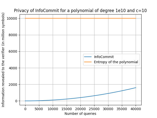
(a) Privacy of Info-Commit.

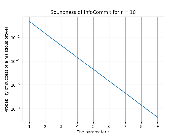
(b) Soundness of Info-Commit.

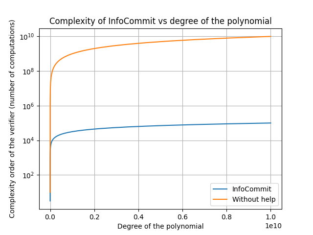
(c) Complexity of verifier relying on Info-Commit.

Figure 1: An illustration of the privacy, soundness and complexity of Info-Commit.

Adaptivity of Info-Commit. Theorem 1 considers the case where the user does not inform the server whether he accepted or rejected the results of the previous queries. We next study the effect of such feedback on the soundness of Info-Commit. Specifically, we consider a setting with $m$ sequential queries $\{x_{1},x_{2},\cdots,x_{m}\}$ such that the user reveals the verification outcome to the server after each round. In such a setting, we show that the soundness guarantee of Info-Commit changes only slightly as given in Theorem 2. The proof closely follows the proof of adaptivity of INTERPOL as presented in [28].

Theorem 2 (Adaptivity of Info-Commit).

In a setting with $m$ sequential queries $\{x_{1},x_{2},\cdots,x_{m}\}$ such that the verification outcome is revealed to the prover after each round, we have

$$\Pr(\exists \ell\in[m]\ \text{s.t.}\ \text{\bf Verify}(x_{\ell},\hat{val}_{\ell},\text{VK},K_{v})=1,$$

$$\hat{val}_{\ell}\neq{val}_{\ell})\leq m\left(\frac{2}{r^{c}}+\frac{1}{r^{2c}}\right),$$ (28)

where $r=|S|/(\sqrt{d}-1)$, $S\subset\mathbb{F}_{q}$ is the prohibited set and $x_{\ell}\notin S,\ell\in[m]$.

The proof of Theorem 2 is provided in Appendix B.

V The Analysis of Info-Commit
(Proof of Theorem 1)

In this section, we prove Theorem 1.

Correctness. If the prover is honest, he will provide the evaluations of the same polynomial $f$ that he initially committed to. Consequently, in the verification phase, (26) holds and the recovered value is equal to $h(x)-g(x)=f(x)$ as desired.
Efficiency. The verification can be done in $O(\sqrt{d})$ since it only requires multiplying $c\times s$ matrices by vectors of length $s=\sqrt{d}$. The recovery can be done in $O(\sqrt{d})$ since the main operation in this phase is inner products of vectors of length $s$. Therefore, the overall complexity of the verifier in the evaluation phase is $O(\sqrt{d})$. The prover, on the other hand, must compute the two vectors $\mathbfsl v$ and $\mathbfsl u$ according to (25) which can be done in $O(d)$.
Soundness. The soundness analysis follows a similar logic as the proof of soundness of INTERPOL [28]. Specifically, the analysis relies on the fact that the prover learns nothing about the secret values $\lambda_{i},\theta_{i}$, $i\in[c]$ during the commitment phase. Note however that unlike Info-Commit, INTERPOL imposed no structural limitation on the secret matrix ${\mathbfsl\Lambda}$. We must show that despite this structural limitation, soundness is guaranteed with overwhelming probability.
Without loss of generality, we can assume that the prover has committed to the correct polynomial $f$. If not, we simply use the letter $f$ to denote the polynomial that the prover has committed to and expect the soundness property to hold with respect to this $f$. Note that such a polynomial of degree $d-1$ exists regardless of how the prover responds to the queries in the commitment phase. Remember that for each input $x$, the prover is required to provide the verifier with two vectors $\mathbfsl v$ and $\mathbfsl u$ as defined in (25). Here, we analyze the probability that a malicious prover can pass the verification test (26) with a $(\hat{\mathbfsl v},\hat{\mathbfsl u})\neq(\mathbfsl v,\mathbfsl u)$ and show that this probability is negligible. Specifically, a malicious prover may respond with (1) $\hat{\mathbfsl v}\neq\mathbfsl v$ and $\hat{\mathbfsl u}=\mathbfsl u$, (2) $\hat{\mathbfsl v}=\mathbfsl v$ and $\hat{\mathbfsl u}\neq\mathbfsl u$ or (3) $\hat{\mathbfsl v}\neq\mathbfsl v$ and $\hat{\mathbfsl u}\neq\mathbfsl u$. Let $({\cal V},{\cal U})$ denote a random variable from which the prover draws the evaluation $(\hat{\mathbfsl v},\hat{\mathbfsl u})$. Note that $({\cal V},{\cal U})$ is independent of $({\mathbfsl\Lambda},{\mathbfsl\Theta})$. We next define these events

$$E_{1}=\{\mathcal{V}\neq\mathbfsl v:\mathbfsl\Lambda(\mathcal{V}-\mathbfsl v)=\mathbfsl 0\},$$ (29)

$$E_{2}=\{\mathcal{U}\neq\mathbfsl u:(\mathcal{U}-\mathbfsl u)\mathbfsl\Theta^{\mathrm{T}}=\mathbfsl 0\}\ \text{and}$$ (30)

$$E_{12}=\{\mathcal{V}\neq\mathbfsl v,\mathcal{U}\neq\mathbfsl u:\mathbfsl\Lambda(\mathcal{V}-\mathbfsl v)=\mathbfsl 0,(\mathcal{U}-\mathbfsl u)\mathbfsl\Theta^{\mathrm{T}}=\mathbfsl 0\}.$$ (31)

The probability that a malicious prover can pass the verification then can be upper-bounded as follows

$$\Pr({\text{\bf Verify}(x,\hat{val},\text{VK},K_{v})=1,\hat{val}\neq val})$$

$$\leq\Pr(E_{1})+\Pr(E_{2})+\Pr(E_{12}).$$ (32)

We first consider the probability of the first event $E_{1}$ as follows

$$p_{\mathbfsl v}\coloneqq\Pr(E_{1})=\Pr\Big{(}\mathbfsl\Lambda({\cal V}-\mathbfsl v)={\bf 0},{\cal V}\neq\mathbfsl v\Big{)},$$ (33)

where the randomness is with respect to $(\mathbfsl\Lambda,{\cal V})$. We need an upper bound on $p_{\mathbfsl v}$ that holds for any $x$ and any $\mathbfsl A,\mathbfsl B$. Define $\begin{bmatrix}\gamma_{0},\cdots,\gamma_{s-1}\end{bmatrix}={\cal V}-\mathbfsl v$ which can be viewed as the coefficients of a polynomial of degree $s-1$, $\gamma(x)=\gamma_{0}+\gamma_{1}x+\cdots+\gamma_{s-1}x^{s-1}$. Equation (33) then represents the probability that the prover can provide a nontrivial polynomial of degree $s-1$ such that all $\lambda_{i}^{s}$, $i\in[c]$, are the roots of this polynomial. Note that the polynomial $\gamma(x)$ has at most $s-1$ roots in the set $S^{\prime}=\{y^{s}|y\in S\}$. Note also that all the terms $\lambda_{i}^{s},i\in[c]$, are distinct. This is because the field size $q$ is chosen in such a way that $\mathrm{gcd}(s,q-1)=1$. As a result, the function $e(x)=x^{s}$ is a permutation, and the set $S^{\prime}$ has $r(s-1)$ distinct elements. Let $T\subseteq S^{\prime}$ be a set of size at most $|T|\leq s-1$ that represents the roots of the polynomial $\gamma(x)$ that are in $S^{\prime}$. In other words, $t\in T$, if and only if $\gamma(t)=0$ and $t\in S^{\prime}$. We are interested in the probability that $\lambda_{i}^{s}\in T$, $\forall i\in[c]$. Since ${\cal V}$ is independent of $\mathbfsl\Lambda$, so is the set $T$. We can therefore upper-bound $p_{\mathbfsl v}$ as follows

$$p_{\mathbfsl v}=\Pr(\lambda_{i}^{s}\in T,\forall i\in[c])\leq\frac{{s-1\choose c}}{{r(s-1)\choose c}}\leq\left(\frac{s-1}{r(s-1)}\right)^{c}=\frac{1}{r^{c}}.$$ (34)

Similarly, one can bound the probability of the second event $E_{2}$ as follows

$$p_{\mathbfsl u}\coloneqq\Pr(E_{2})=\Pr\left((\cal U-\mathbfsl u)\mathbfsl\Theta^{\mathrm{T}}=\mathbfsl 0,{\cal U}\neq\mathbfsl u\right)\leq\frac{1}{r^{c}}.$$ (35)

Finally, the probability of $E_{12}$ can be also upper-bounded as

$$p_{\mathbfsl v,\mathbfsl u}\coloneqq\Pr(E_{12})\leq\frac{1}{r^{2c}}.$$ (36)

As a result, we have

$$\Pr({\text{\bf Verify}(x,\hat{val},\text{VK},K_{v})=1,\hat{val}\neq val})\leq\frac{2}{r^{c}}+\frac{1}{r^{2c}}.$$ (37)

For instance, by choosing $r=10$ and $c=10$, this probability can be reduced to $\approx 2\times 10^{-10}$.

We now study the privacy of Info-Commit. We begin with the following useful lemmas that will help us establish the privacy of Info-Commit.

Lemma 1.

Let $c,d,s$ be three positive integers such that $c,d\leq s$. Let $\mathbfsl E$ be an $s\times s$ random matrix uniformly distributed over $\mathbb{F}_{q}^{s\times s}$. Let $\mathbfsl F$ and $\mathbfsl G$ be arbitrary full-rank $c\times s$ and $s\times d$ matrices respectively. Then

$$H_{q}(\mathbfsl F\mathbfsl E|\mathbfsl E\mathbfsl G)\geq cs-cd.$$ (38)

Proof.

Since $\mathbfsl G$ is a full-rank matrix, then the matrix $\mathbfsl E\mathbfsl G$ is uniformly distributed over $\mathbb{F}_{q}^{s\times d}$ and as a result, $H_{q}(\mathbfsl E\mathbfsl G)=sd$. So, we only need to prove that

$$H_{q}(\mathbfsl F\mathbfsl E,\mathbfsl E\mathbfsl G)\geq cs+sd-cd.$$ (39)

Let $\boldsymbol{\ell}\in\mathbb{F}_{q}^{s^{2}}$ be a column vector obtained from the vertical concatenation of the columns of $\mathbfsl E$, such that $\ell_{i+sj}=E_{i,j}$ for all $i\in[0:s-1]$, $j\in[0:s-1]$. Let $\mathbfcal F=\mathbf{I}_{s\times s}\otimes\mathbfsl F$ and $\mathbfcal G=\mathbfsl G\otimes\mathbf{I}_{s\times s}$, where $\mathbf{I}_{s\times s}$ is the $s\times s$ identity matrix and $\otimes$ denotes the Kronecker product. Since the two vectors $\mathbfcal F\boldsymbol{\ell}$ and $\mathbfcal G\boldsymbol{\ell}$ are rearrangements of the the two matrices $\mathbfsl F\mathbfsl E$ and $\mathbfsl E\mathbfsl G$, respectively, we have

$$H_{q}(\mathbfsl F\mathbfsl E,\mathbfsl E\mathbfsl G)=H_{q}(\mathbfcal F\boldsymbol{\ell},\mathbfcal G\boldsymbol{\ell}).$$ (40)

The proof follows from the fact that the $(c+d)s\times s^{2}$ matrix $\mathbfcal H=\mathbfcal F||\mathbfcal G$ obtained from vertical concatenation of $\mathbfcal F$ and $\mathbfcal G$ has rank at least $(c+d)s-cd$ as long as $\mathbfsl F$ and $\mathbfsl G$ are full-rank (See Lemma 3 in Appendix A). ∎

Lemma 2.

Let $E,F,G$ be three random variables with alphabets ${\cal E},{\cal F},{\cal G}$, satisfying the Markov chain $E\longleftrightarrow F\longleftrightarrow G$. Let $h:{\cal E}\times{\cal G}\rightarrow{\cal W}$ be an arbitrary function. Then, we have

$$H(E|F,h(E,G))\geq\min_{g\in{\cal G}}H(E|F,h(E,g)).$$ (41)

Proof.

The following chain of inequalities proves the claim

$$H(E|F,h(E,G))\geq H(E|F,G,h(E,G))$$ (42)

$$=\sum_{g\in{\cal G}}\Pr(G=g)H(E|F,G=g,h(E,g))$$ (43)

$$\geq\min_{g\in{\cal G}}H(E|F,G=g,h(E,g))=\min_{g\in{\cal G}}H(E|F,h(E,g)),$$ (44)

where the last inequality follows from Property 1 in the preliminaries. Specifically, since $E\longleftrightarrow F\longleftrightarrow G$ forms a Markov chain, then $E\longleftrightarrow(F,h(E,g))\longleftrightarrow G$ forms a Markov chain too, which allows us to drop $G=g$ from conditioning. ∎

Privacy. We now prove that after $m$ evaluations, the verifier learns at most $(m+c)^{2}$ symbols over $\mathbb{F}_{q}$ about the matrix $\mathbfsl A$ which represents the polynomial $f$. The analysis of privacy relies on the fact that the verifier learns nothing about $(\mathbfsl A+\mathbfsl B,\mathbfsl B)$ in the commitment phase except for what is implied via $(\mathbfsl\Gamma,\mathbfsl\Omega)$. The analysis also makes use of the fact that the $\lambda_{i}$ and $\theta_{i}$ values in the commitment phase are chosen from a “prohibited" set. As a result of this, the matrices $\mathbfsl\Lambda||\mathbfsl Y$ and $\mathbfsl\Theta||\mathbfsl X$ will be full-rank. Note that the verifier cannot benefit from selecting $x_{i}=x_{j}$, i.e., requesting the same evaluation point twice. Similarly, he cannot benefit from setting $\lambda_{i}=\lambda_{j}$ or $\theta_{i}=\theta_{j}$. Therefore, without loss of generality, we can assume that $\operatorname{rank}(\mathbfsl\Lambda||\mathbfsl Y)=\operatorname{rank}(\mathbfsl\Theta||\mathbfsl X)=m+c$.
For $(\mathbfsl X,\mathbfsl Y,\mathbfsl V,\mathbfsl U)$ defined as in (15),(16), we want to show that

$$H_{q}(\mathbfsl A|\mathbfsl V,\mathbfsl U,\mathbfsl\Gamma,\mathbfsl\Omega)\geq d-(m+c)^{2},$$ (45)

for any choice of the evaluation points $x_{1},\cdots,x_{m}$ and for any choice of $\theta_{1},\cdots,\theta_{c},$ $\lambda_{1},\cdots,\lambda_{c}$. We start by simplifying the left-hand side of (45) as follows

$$H_{q}(\mathbfsl A|\mathbfsl V,\mathbfsl U,\mathbfsl\Gamma,\mathbfsl\Omega)=H_{q}(\mathbfsl A|(\mathbfsl A+\mathbfsl B)\mathbfsl X^{\mathrm{T}},\mathbfsl Y\mathbfsl B,\mathbfsl\Lambda(\mathbfsl A+\mathbfsl B),\mathbfsl B\mathbfsl\Theta^{\mathrm{T}})$$

$$=H_{q}(\mathbfsl A,(\mathbfsl A+\mathbfsl B)\mathbfsl X^{\mathrm{T}},\mathbfsl\Lambda(\mathbfsl A+\mathbfsl B)|(\mathbfsl A+\mathbfsl B)\mathbfsl X^{\mathrm{T}},\mathbfsl Y\mathbfsl B,\mathbfsl\Lambda(\mathbfsl A+\mathbfsl B),\mathbfsl B\mathbfsl\Theta^{\mathrm{T}})$$

$$=H_{q}(\mathbfsl A,\mathbfsl B\mathbfsl X^{\mathrm{T}},\mathbfsl\Lambda\mathbfsl B|(\mathbfsl A+\mathbfsl B)\mathbfsl X^{\mathrm{T}},\mathbfsl Y\mathbfsl B,\mathbfsl\Lambda(\mathbfsl A+\mathbfsl B),\mathbfsl B\mathbfsl\Theta^{\mathrm{T}})$$

$$=H_{q}(\mathbfsl B\mathbfsl X^{\mathrm{T}},\mathbfsl\Lambda\mathbfsl B|(\mathbfsl A+\mathbfsl B)\mathbfsl X^{\mathrm{T}},\mathbfsl Y\mathbfsl B,\mathbfsl\Lambda(\mathbfsl A+\mathbfsl B),\mathbfsl B\mathbfsl\Theta^{\mathrm{T}})$$

$$+H_{q}(\mathbfsl A|\mathbfsl B\mathbfsl X^{\mathrm{T}},\mathbfsl\Lambda\mathbfsl B,(\mathbfsl A+\mathbfsl B)\mathbfsl X^{\mathrm{T}},\mathbfsl Y\mathbfsl B,\mathbfsl\Lambda(\mathbfsl A+\mathbfsl B),\mathbfsl B\mathbfsl\Theta^{\mathrm{T}})$$

$$=H_{q}(\mathbfsl B\mathbfsl X^{\mathrm{T}},\mathbfsl\Lambda\mathbfsl B|(\mathbfsl A+\mathbfsl B)\mathbfsl X^{\mathrm{T}},\mathbfsl Y\mathbfsl B,\mathbfsl\Lambda(\mathbfsl A+\mathbfsl B),\mathbfsl B\mathbfsl\Theta^{\mathrm{T}})+$$

$$H_{q}(\mathbfsl A|\mathbfsl A\mathbfsl X^{\mathrm{T}},\mathbfsl\Lambda\mathbfsl A),$$ (46)

where the last equality follows from the fact that $\mathbfsl A$ is independent of $\mathbfsl B$. The second term in the final expression can be easily bounded as

$$H_{q}(\mathbfsl A|\mathbfsl A\mathbfsl X^{\mathrm{T}},\mathbfsl\Lambda\mathbfsl A) =H_{q}(\mathbfsl A)-H_{q}(\mathbfsl A\mathbfsl X^{\mathrm{T}},\mathbfsl\Lambda\mathbfsl A)$$

$$\geq H_{q}(\mathbfsl A)-H_{q}(\mathbfsl A\mathbfsl X^{\mathrm{T}})-H_{q}(\mathbfsl\Lambda\mathbfsl A)$$

$$=d-ms-cs.$$ (47)

Therefore, we must show that the first term satisfies

$$H_{q}(\mathbfsl B\mathbfsl X^{\mathrm{T}},\mathbfsl\Lambda\mathbfsl B|(\mathbfsl A+\mathbfsl B)\mathbfsl X^{\mathrm{T}},\mathbfsl Y\mathbfsl B,\mathbfsl\Lambda(\mathbfsl A+\mathbfsl B),\mathbfsl B\mathbfsl\Theta^{\mathrm{T}})$$

$$\geq ms+cs-(m+c)^{2}.$$ (48)

Observe that $\Big{(}(\mathbfsl A+\mathbfsl B)\mathbfsl X^{\mathrm{T}},\mathbfsl\Lambda(\mathbfsl A+\mathbfsl B)\Big{)}$ is independent of $\Big{(}\mathbfsl B\mathbfsl X^{\mathrm{T}},\mathbfsl\Lambda\mathbfsl B,\mathbfsl Y\mathbfsl B,\mathbfsl B\mathbfsl\Theta^{\mathrm{T}}\Big{)}$. This follows as $\mathbfsl A+\mathbfsl B$ is independent of $\mathbfsl B$. Hence, following basic properties of the entropy function, we have

$$H_{q}(\mathbfsl B\mathbfsl X^{\mathrm{T}},\mathbfsl\Lambda\mathbfsl B|(\mathbfsl A+\mathbfsl B)\mathbfsl X^{\mathrm{T}},\mathbfsl Y\mathbfsl B,\mathbfsl\Lambda(\mathbfsl A+\mathbfsl B),\mathbfsl B\mathbfsl\Theta^{\mathrm{T}})$$

$$=H_{q}(\mathbfsl B\mathbfsl X^{\mathrm{T}},\mathbfsl\Lambda\mathbfsl B|\mathbfsl Y\mathbfsl B,\mathbfsl B\mathbfsl\Theta^{\mathrm{T}}).$$ (49)

It remains to prove that

$$H_{q}(\mathbfsl B\mathbfsl X^{\mathrm{T}},\mathbfsl\Lambda\mathbfsl B|\mathbfsl Y\mathbfsl B,\mathbfsl B\mathbfsl\Theta^{\mathrm{T}})\geq ms+cs-(m+c)^{2}.$$ (50)

Note that

$$H_{q}(\mathbfsl B\mathbfsl X^{\mathrm{T}},\mathbfsl\Lambda\mathbfsl B|\mathbfsl Y\mathbfsl B,\mathbfsl B\mathbfsl\Theta^{\mathrm{T}})$$

$$=H_{q}(\mathbfsl B\mathbfsl X^{\mathrm{T}},\mathbfsl\Lambda\mathbfsl B,\mathbfsl Y\mathbfsl B,\mathbfsl B\mathbfsl\Theta^{\mathrm{T}})-H_{q}(\mathbfsl Y\mathbfsl B,\mathbfsl B\mathbfsl\Theta^{\mathrm{T}})$$

$$=H_{q}(\mathbfsl B\mathbfsl X^{\mathrm{T}},\mathbfsl B\mathbfsl\Theta^{\mathrm{T}})+H_{q}(\mathbfsl\Lambda\mathbfsl B,\mathbfsl Y\mathbfsl B|\mathbfsl B\mathbfsl X^{\mathrm{T}},\mathbfsl B\mathbfsl\Theta^{\mathrm{T}})$$

$$-H_{q}(\mathbfsl Y\mathbfsl B,\mathbfsl B\mathbfsl\Theta^{\mathrm{T}}).$$ (51)

Due to the fact that $x_{i}$ and $\theta_{i}$ values are chosen from two different sets, we know that $\mathbfsl\Theta||\mathbfsl X$ is a full-rank matrix. Therefore, we have

$$H_{q}(\mathbfsl B\mathbfsl X^{\mathrm{T}},\mathbfsl B\mathbfsl\Theta^{\mathrm{T}})=(c+m)s.$$ (52)

Similarly, the matrix $\mathbfsl\Lambda||\mathbfsl Y$ is full-rank, thus by Lemma 1

$$H_{q}(\mathbfsl\Lambda\mathbfsl B,\mathbfsl Y\mathbfsl B|\mathbfsl B\mathbfsl X^{\mathrm{T}},\mathbfsl B\mathbfsl\Theta^{\mathrm{T}})\geq(c+m)s-(c+m)^{2}.$$ (53)

Also, we have

$$H_{q}(\mathbfsl Y\mathbfsl B,\mathbfsl B\mathbfsl\Theta^{\mathrm{T}})\leq H_{q}(\mathbfsl Y\mathbfsl B)+H_{q}(\mathbfsl B\mathbfsl\Theta^{\mathrm{T}})=ms+cs.$$ (54)

Therefore, we have

$$H_{q}(\mathbfsl B\mathbfsl X^{\mathrm{T}},\mathbfsl\Lambda\mathbfsl B|\mathbfsl Y\mathbfsl B,\mathbfsl B\mathbfsl\Theta^{\mathrm{T}})\geq ms+cs-(m+c)^{2}.$$ (55)

This gives us the desired inequality $H_{q}(\mathbfsl A|\mathbfsl V,\mathbfsl U,\mathbfsl\Gamma,\mathbfsl\Omega)\geq d-(m+c)^{2}$.
We proved that $H_{q}(\mathbfsl A|(\mathbfsl A+\mathbfsl B)\mathbfsl X^{\mathrm{T}},\mathbfsl Y\mathbfsl B,\mathbfsl\Gamma,\mathbfsl\Omega)\geq d-(m+c)^{2}$, for every choice of the evaluation points $x_{1},\cdots,x_{m}$. Note that in general, the verifier may choose the evaluation points after observing the commitment ${(\mathbfsl\Gamma,\mathbfsl\Omega)}$. In other words, rather than assuming $(\mathbfsl X,\mathbfsl Y)$ are arbitrary constants, we must treat them as random variables satisfying the following Markov chain

$$(\mathbfsl A,\mathbfsl B)\longleftrightarrow(\mathbfsl\Gamma,\mathbfsl\Omega)\longleftrightarrow(\mathbfsl X,\mathbfsl Y).$$ (56)

But thanks to Lemma 2, since $(\mathbfsl\Gamma,\mathbfsl\Omega)$ appear in the conditioning, we have

$$H_{q}(\mathbfsl A|(\mathbfsl A+\mathbfsl B)\mathbfsl X^{\mathrm{T}},\mathbfsl Y\mathbfsl B,\mathbfsl\Gamma,\mathbfsl\Omega)\geq$$

$$\min_{x_{1},\cdots,x_{m}}H_{q}(\mathbfsl A|(\mathbfsl A+\mathbfsl B)\begin{bmatrix}1&x_{1}&\cdots&x_{1}^{s-1}\\ &\cdots&\cdots&\\ 1&x_{m}&\cdots&x_{m}^{s-1}\end{bmatrix}^{\mathrm{T}},$$

$$\begin{bmatrix}1&x_{1}^{s}&\cdots&x_{1}^{s(s-1)}\\ &\cdots&\cdots&\\ 1&x_{m}^{s}&\cdots&x_{m}^{s(s-1)}\end{bmatrix}\mathbfsl B,\mathbfsl\Gamma,\mathbfsl\Omega).$$ (57)

Therefore, the analysis we provided also addresses the case where the evaluation points are chosen adaptively, after observing the commitment.

VI Conclusions

In this work, we have developed Info-Commit, an information-theoretic protocol for polynomial commitment and verification. Specifically, we have considered a setting with an untrusted server (prover) hosting a private polynomial $f$ of degree $d-1$ and a user (verifier) who wishes to obtain evaluations of $f$. Info-Commit consists of a commitment phase, in which the user learns a private commitment to the prover’s polynomial, and an evaluation phase. Info-Commit only requires a trusted third-party in the commitment phase, provides unconditional privacy guarantees for the server and unconditional verifiability for the user irrespective of their computational power. Moreover, Info-Commit is doubly-efficient with an efficient prover of complexity $O(d)$ and a super-efficient verifier with complexity of $O(\sqrt{d})$.

Appendix A Lemma 3

Lemma 3.

Let $c,d,s$ be three positive integers such that $c,d\leq s$. Let $\mathbfsl F$ and $\mathbfsl G$ be two full-rank $c\times s$ and $d\times s$ matrices over $\mathbb{F}_{q}$, respectively. Let $\mathbfcal F=\mathbfsl{I}_{s\times s}\otimes\mathbfsl F$, $\mathbfcal G={\mathbfsl G}\otimes\mathbfsl{I}_{s\times s}$ and let $\mathbfcal H={\mathbfcal F}||{\mathbfcal G}$ be the $(c+d)s\times s^{2}$ matrix obtained from vertical concatenation of ${\mathbfcal F}$ and ${\mathbfcal G}$. Then, we have

$$\operatorname{rank}({\mathbfcal H})\geq(c+d)s-cd.$$ (58)

Proof.

Since $\mathbfsl F$ is full-rank and $c\leq s$, $\mathbfsl F$ must have at least one $c\times c$ full-rank submatrix. Let $\tau\subseteq[0:s-1]$ represent the indices of the columns of one such sub-matrix and let $\mathbfsl F_{\tau}$ be the corresponding submatrix of $\mathbfsl F$. We also define

$$\rho=\{cs+i+sj|j\in[0:d-1],i\in\tau\}.$$ (59)

Intuitively, $\rho$ corresponds to the rows of ${\mathbfcal G}$ which may have a non-zero element in any column from ${\tau}$. Note that $|\rho|=cd$. We will argue that by eliminating the rows indexed in $\rho$ from ${\mathbfcal H}$, we will find a full-rank matrix. Since this resulting matrix has ${(c+d)s-cd}$ rows, the claim will follow. In Equation (60) below, we have illustrated an example with $s=4,c=3$ and $d=2$. We have assumed that ${\tau}=\{1,2,3\}$ and have marked the full-rank submatrix of $\mathbfsl F$ in blue. The rows indexed in $\rho$ are shown in red.

Let $\boldsymbol{\lambda}$ be a vector of length $(c+d)s$ such that $\lambda_{i}=0,\forall i\in\rho$ and $\boldsymbol{\lambda}{\mathbfcal H}={\bf 0}$. We will show that ${\boldsymbol{\lambda}}$ must be the all-zero vector. For $j\in[0:s-1]$, let ${\mathbfcal H}_{j}$ be the submatrix of ${\mathbfcal H}$ obtained from columns $\{i+sj|i+cs\in\rho\}$. Since $\boldsymbol{\lambda}{\mathbfcal H}={\bf 0}$, we must have $\boldsymbol{\lambda}{\mathbfcal H}_{j}={\bf 0}$. But for any $i\in[0:(c+d)s-1]\backslash[jc:(j+1)c-1]$, either $\lambda_{i}=0$ or the $i$’th row of ${\mathbfcal H}_{j}$ is an all-zero vector. It follows that $\boldsymbol{\lambda}_{[jc:(j+1)c-1]}\mathbfsl F_{\tau}={\bf 0}$. But $\mathbfsl F_{\tau}$ is full-rank, so $\boldsymbol{\lambda}_{[jc:(j+1)c-1]}={\bf 0}$. Since this holds for every $j\in[0:s-1]$, we conclude that $\boldsymbol{\lambda}_{[0:cs-1]}={\bf 0}$.

It follows from $\boldsymbol{\lambda}_{[0:cs-1]}={\bf 0}$ and $\boldsymbol{\lambda}{\mathbfcal H}={\bf 0}$ that $\boldsymbol{\lambda}_{[cs:(c+d)s-1]}{\mathbfcal G}={\bf 0}$. Define the $s\times d$ matrix $\boldsymbol{\theta}$ such that $\theta_{i,j}=\lambda_{i+sj}$. Observe that $\boldsymbol{\lambda}_{[cs:(c+d)s-1]}{\mathbfcal G}$ is a vector found by rearranging the elements of the matrix $\boldsymbol{\theta}\mathbfsl G$. Since $\boldsymbol{\lambda}_{[cs:(c+d)s-1]}{\mathbfcal G}={\bf 0}$, we must have $\boldsymbol{\theta}\mathbfsl G={\bf 0}$. Since $\mathbfsl G$ is full-rank, it follows that $\boldsymbol{=}{\bf 0}$ and as a result $\boldsymbol{\lambda}_{[cs:(c+d)s-1]}={\bf 0}$. We conclude that $\boldsymbol{\lambda}={\bf 0}$ which establishes the claim. ∎

$${\mathbfcal H}=\setcounter{MaxMatrixCols}{16}\begin{bmatrix}f_{0,0}&{\color[rgb]{0,0,1}f_{0,1}}&{\color[rgb]{0,0,1}f_{0,2}}&{\color[rgb]{0,0,1}f_{0,3}}&0&0&0&0&0&0&0&0&0&0&0&0\\ f_{1,0}&{\color[rgb]{0,0,1}f_{1,1}}&{\color[rgb]{0,0,1}f_{1,2}}&{\color[rgb]{0,0,1}f_{1,3}}&0&0&0&0&0&0&0&0&0&0&0&0\\ f_{2,0}&{\color[rgb]{0,0,1}f_{2,1}}&{\color[rgb]{0,0,1}f_{2,2}}&{\color[rgb]{0,0,1}f_{2,3}}&0&0&0&0&0&0&0&0&0&0&0&0\\ 0&0&0&0&f_{0,0}&{\color[rgb]{0,0,1}f_{0,1}}&{\color[rgb]{0,0,1}f_{0,2}}&{\color[rgb]{0,0,1}f_{0,3}}&0&0&0&0&0&0&0&0\\ 0&0&0&0&f_{1,0}&{\color[rgb]{0,0,1}f_{1,1}}&{\color[rgb]{0,0,1}f_{1,2}}&{\color[rgb]{0,0,1}f_{1,3}}&0&0&0&0&0&0&0&0\\ 0&0&0&0&f_{2,0}&{\color[rgb]{0,0,1}f_{2,1}}&{\color[rgb]{0,0,1}f_{2,2}}&{\color[rgb]{0,0,1}f_{2,3}}&0&0&0&0&0&0&0&0\\ 0&0&0&0&0&0&0&0&f_{0,0}&{\color[rgb]{0,0,1}f_{0,1}}&{\color[rgb]{0,0,1}f_{0,2}}&{\color[rgb]{0,0,1}f_{0,3}}&0&0&0&0\\ 0&0&0&0&0&0&0&0&f_{1,0}&{\color[rgb]{0,0,1}f_{1,1}}&{\color[rgb]{0,0,1}f_{1,2}}&{\color[rgb]{0,0,1}f_{1,3}}&0&0&0&0\\ 0&0&0&0&0&0&0&0&f_{2,0}&{\color[rgb]{0,0,1}f_{2,1}}&{\color[rgb]{0,0,1}f_{2,2}}&{\color[rgb]{0,0,1}f_{2,3}}&0&0&0&0\\ 0&0&0&0&0&0&0&0&0&0&0&0&f_{0,0}&{\color[rgb]{0,0,1}f_{0,1}}&{\color[rgb]{0,0,1}f_{0,2}}&{\color[rgb]{0,0,1}f_{0,3}}\\ 0&0&0&0&0&0&0&0&0&0&0&0&f_{1,0}&{\color[rgb]{0,0,1}f_{1,1}}&{\color[rgb]{0,0,1}f_{1,2}}&{\color[rgb]{0,0,1}f_{1,3}}\\ 0&0&0&0&0&0&0&0&0&0&0&0&f_{2,0}&{\color[rgb]{0,0,1}f_{2,1}}&{\color[rgb]{0,0,1}f_{2,2}}&{\color[rgb]{0,0,1}f_{2,3}}\\ g_{0,0}&0&0&0&g_{0,1}&0&0&0&g_{0,2}&0&0&0&g_{0,3}&0&0&0\\ {\color[rgb]{1,0,0}0}&{\color[rgb]{1,0,0}g_{0,0}}&{\color[rgb]{1,0,0}0}&{\color[rgb]{1,0,0}0}&{\color[rgb]{1,0,0}0}&{\color[rgb]{1,0,0}g_{0,1}}&{\color[rgb]{1,0,0}0}&{\color[rgb]{1,0,0}0}&{\color[rgb]{1,0,0}0}&{\color[rgb]{1,0,0}g_{0,2}}&{\color[rgb]{1,0,0}0}&{\color[rgb]{1,0,0}0}&{\color[rgb]{1,0,0}0}&{\color[rgb]{1,0,0}g_{0,3}}&{\color[rgb]{1,0,0}0}&{\color[rgb]{1,0,0}0}\\ {\color[rgb]{1,0,0}0}&{\color[rgb]{1,0,0}0}&{\color[rgb]{1,0,0}g_{0,0}}&{\color[rgb]{1,0,0}0}&{\color[rgb]{1,0,0}0}&{\color[rgb]{1,0,0}0}&{\color[rgb]{1,0,0}g_{0,1}}&{\color[rgb]{1,0,0}0}&{\color[rgb]{1,0,0}0}&{\color[rgb]{1,0,0}0}&{\color[rgb]{1,0,0}g_{0,2}}&{\color[rgb]{1,0,0}0}&{\color[rgb]{1,0,0}0}&{\color[rgb]{1,0,0}0}&{\color[rgb]{1,0,0}g_{0,3}}&{\color[rgb]{1,0,0}0}\\ {\color[rgb]{1,0,0}0}&{\color[rgb]{1,0,0}0}&{\color[rgb]{1,0,0}0}&{\color[rgb]{1,0,0}g_{0,0}}&{\color[rgb]{1,0,0}0}&{\color[rgb]{1,0,0}0}&{\color[rgb]{1,0,0}0}&{\color[rgb]{1,0,0}g_{0,1}}&{\color[rgb]{1,0,0}0}&{\color[rgb]{1,0,0}0}&{\color[rgb]{1,0,0}0}&{\color[rgb]{1,0,0}g_{0,2}}&{\color[rgb]{1,0,0}0}&{\color[rgb]{1,0,0}0}&{\color[rgb]{1,0,0}0}&{\color[rgb]{1,0,0}g_{0,3}}\\ g_{1,0}&0&0&0&g_{1,1}&0&0&0&g_{1,2}&0&0&0&g_{1,3}&0&0&0\\ {\color[rgb]{1,0,0}0}&{\color[rgb]{1,0,0}g_{1,0}}&{\color[rgb]{1,0,0}0}&{\color[rgb]{1,0,0}0}&{\color[rgb]{1,0,0}0}&{\color[rgb]{1,0,0}g_{1,1}}&{\color[rgb]{1,0,0}0}&{\color[rgb]{1,0,0}0}&{\color[rgb]{1,0,0}0}&{\color[rgb]{1,0,0}g_{1,2}}&{\color[rgb]{1,0,0}0}&{\color[rgb]{1,0,0}0}&{\color[rgb]{1,0,0}0}&{\color[rgb]{1,0,0}g_{1,3}}&{\color[rgb]{1,0,0}0}&{\color[rgb]{1,0,0}0}\\ {\color[rgb]{1,0,0}0}&{\color[rgb]{1,0,0}0}&{\color[rgb]{1,0,0}g_{1,0}}&{\color[rgb]{1,0,0}0}&{\color[rgb]{1,0,0}0}&{\color[rgb]{1,0,0}0}&{\color[rgb]{1,0,0}g_{1,1}}&{\color[rgb]{1,0,0}0}&{\color[rgb]{1,0,0}0}&{\color[rgb]{1,0,0}0}&{\color[rgb]{1,0,0}g_{1,2}}&{\color[rgb]{1,0,0}0}&{\color[rgb]{1,0,0}0}&{\color[rgb]{1,0,0}0}&{\color[rgb]{1,0,0}g_{1,3}}&{\color[rgb]{1,0,0}0}\\ {\color[rgb]{1,0,0}0}&{\color[rgb]{1,0,0}0}&{\color[rgb]{1,0,0}0}&{\color[rgb]{1,0,0}g_{1,0}}&{\color[rgb]{1,0,0}0}&{\color[rgb]{1,0,0}0}&{\color[rgb]{1,0,0}0}&{\color[rgb]{1,0,0}g_{1,1}}&{\color[rgb]{1,0,0}0}&{\color[rgb]{1,0,0}0}&{\color[rgb]{1,0,0}0}&{\color[rgb]{1,0,0}g_{1,2}}&{\color[rgb]{1,0,0}0}&{\color[rgb]{1,0,0}0}&{\color[rgb]{1,0,0}0}&{\color[rgb]{1,0,0}b_{1,3}}\end{bmatrix}.$$ (60)

Appendix B Adaptivity of Info-Commit
(Proof of Theorem 2)

We now provide the proof of Theorem 2.

Proof.

Suppose that an adversarial server responds with $\mathcal{V}_{\ell}=\mathbfsl v_{\ell}+\mathcal{W}_{\ell}$ and $\mathcal{U}_{\ell}=\mathbfsl u_{\ell}+\mathcal{Z}_{\ell}$, where $(\mathcal{W}_{l},\mathcal{Z}_{l})\neq(\mathbfsl 0,\mathbfsl 0)$. That is, the server returns at least one incorrect computation. Since the server is informed whether the computation outcome is accepted or not after each evaluation, then we have the following Markov property

$$(\mathbfsl\Lambda,\mathbfsl\Theta)\leftrightarrow(V_{1},V_{2},\cdots,V_{\ell-1})\leftrightarrow(\mathcal{W}_{\ell},\mathcal{Z}_{\ell}),$$ (61)

where $V_{\ell}=\mathbf{1}(\mathbfsl\Lambda\mathcal{W}_{\ell}=\mathbfsl 0,\mathcal{Z}_{\ell}\mathbfsl\Theta^{\mathrm{T}}=\mathbfsl 0)$. The probability that the server fails all verifications in all $m$ rounds can be expressed as follows

$$P_{m} =\Pr\left(V_{m}=0,V_{m-1}=0\cdots,V_{1}=0\right)$$

$$=\Pr\left(V_{m}=0|V_{m-1}=0\cdots,V_{1}=0\right)P_{m-1}.$$ (62)

The first term can be lower-bounded as follows

$$T_{m}\coloneqq\Pr\left(V_{m}=0|V_{m-1}=0\cdots,V_{1}=0\right)$$

$$=\sum_{(\mathbfsl w_{m},\mathbfsl z_{m})\neq(\mathbfsl 0,\mathbfsl 0)}\Pr\left((\mathbfsl\Lambda\mathcal{W}_{m}\neq\mathbfsl 0)\cup(\mathcal{Z}_{m}\mathbfsl\Theta^{\mathrm{T}}\neq\mathbfsl 0)|\right.$$

$$~{}~{}~{}~{}~{}~{}~{}\left.(\mathcal{W}_{m},\mathcal{Z}_{m})=(\mathbfsl w_{m},\mathbfsl z_{m}),V_{m-1}=0,\cdots,V_{1}=0\right)$$

$$~{}~{}~{}~{}~{}~{}~{}~{}~{}~{}~{}~{}~{}~{}~{}~{}\Pr((\mathcal{W}_{m},\mathcal{Z}_{m})=(\mathbfsl w_{m},\mathbfsl z_{m})|V_{m-1}=0,\cdots,V_{1}=0)$$

$$=\sum_{(\mathbfsl w_{m},\mathbfsl z_{m})\neq(\mathbfsl 0,\mathbfsl 0)}\Pr\left((\mathbfsl\Lambda\mathbfsl w_{m}\neq\mathbfsl 0)\cup(\mathbfsl z_{m}\mathbfsl\Theta^{\mathrm{T}}\neq\mathbfsl 0)|\right.$$

$$\left.~{}~{}~{}~{}~{}~{}~{}~{}~{}~{}~{}~{}~{}~{}~{}~{}~{}~{}~{}~{}~{}~{}~{}~{}~{}~{}V_{m-1}=0,\cdots,V_{1}=0\right)$$

$$~{}~{}~{}~{}~{}~{}~{}~{}~{}~{}~{}~{}~{}~{}~{}~{}~{}~{}~{}~{}\Pr((\mathcal{W}_{m},\mathcal{Z}_{m})=(\mathbfsl w_{m},\mathbfsl z_{m})|V_{m-1}=0,\cdots,V_{1}=0),$$ (63)

where the last equality follows from the Markov property in (61). The first term inside this summation can be bounded as

$$R_{m} \coloneqq\Pr\left((\mathbfsl\Lambda\mathbfsl w_{m}\neq\mathbfsl 0)\cup(\mathbfsl z_{m}\mathbfsl\Theta^{\mathrm{T}}\neq\mathbfsl 0)|V_{m-1}=0,\cdots,V_{1}=0\right)$$

$$=1-\Pr\left(\mathbfsl\Lambda\mathbfsl w_{m}=\mathbfsl 0,\mathbfsl z_{m}\mathbfsl\Theta^{\mathrm{T}}=\mathbfsl 0|V_{m-1}=0,\cdots,V_{1}=0\right)$$

$$=1-\frac{\Pr\left(\mathbfsl\Lambda\mathbfsl w_{m}=\mathbfsl 0,\mathbfsl z_{m}\mathbfsl\Theta^{\mathrm{T}}=\mathbfsl 0,V_{m-1}=0,\cdots,V_{1}=0\right)}{P_{m-1}}$$

$$\geq 1-\frac{\Pr\left(\mathbfsl\Lambda\mathbfsl w_{m}=\mathbfsl 0,\mathbfsl z_{m}\mathbfsl\Theta^{\mathrm{T}}=\mathbfsl 0\right)}{P_{m-1}}$$

$$\geq 1-\frac{1}{P_{m-1}}\left(\frac{2}{r^{c}}+\frac{1}{r^{2c}}\right).$$ (64)

Hence, we have

$$T_{m}\geq 1-\frac{1}{P_{m-1}}\left(\frac{2}{r^{c}}+\frac{1}{r^{2c}}\right)$$ (65)

and

$$P_{m} =T_{m}P_{m-1}$$

$$\geq P_{m-1}-\left(\frac{2}{r^{c}}+\frac{1}{r^{2c}}\right)$$

$$\geq P_{1}-(m-1)\left(\frac{2}{r^{c}}+\frac{1}{r^{2c}}\right)$$

$$\geq 1-m\left(\frac{2}{r^{c}}+\frac{1}{r^{2c}}\right),$$ (66)

where the last inequality follows since $P_{1}\geq 1-\left(\frac{2}{r^{c}}+\frac{1}{r^{2c}}\right)$. Hence, we have

$$\Pr( \exists\ell\in[m]\ \text{s.t.}\ \text{\bf Verify}(x_{\ell},\hat{val}_{\ell},\text{VK},K_{v})=1,\hat{val}_{\ell}\neq{val}_{\ell})$$

$$\leq m\left(\frac{2}{r^{c}}+\frac{1}{r^{2c}}\right).$$ (67)

∎

References

• [1] S. Goldwasser, Y. T. Kalai, and G. N. Rothblum, “Delegating computation: interactive proofs for muggles,” in Proceedings of the fortieth annual ACM symposium on Theory of computing.   ACM, 2008, pp. 113–122.
• [2] R. Gennaro, C. Gentry, and B. Parno, “Non-interactive verifiable computing: Outsourcing computation to untrusted workers,” in Annual Cryptology Conference.   Springer, 2010, pp. 465–482.
• [3] S. Benabbas, R. Gennaro, and Y. Vahlis, “Verifiable delegation of computation over large datasets,” in Annual Cryptology Conference.   Springer, 2011, pp. 111–131.
• [4] D. Fiore and R. Gennaro, “Publicly verifiable delegation of large polynomials and matrix computations, with applications,” in Proceedings of the 2012 ACM conference on Computer and communications security.   ACM, 2012, pp. 501–512.
• [5] B. Libert, S. C. Ramanna, and M. Yung, “Functional commitment schemes: From polynomial commitments to pairing-based accumulators from simple assumptions,” in 43rd International Colloquium on Automata, Languages, and Programming (ICALP 2016).   Schloss Dagstuhl-Leibniz-Zentrum fuer Informatik, 2016.
• [6] A. Kate, G. M. Zaverucha, and I. Goldberg, “Constant-size commitments to polynomials and their applications,” in International Conference on the Theory and Application of Cryptology and Information Security.   Springer, 2010, pp. 177–194.
• [7] S. Li, M. Yu, C.-S. Yang, A. S. Avestimehr, S. Kannan, and P. Viswanath, “Polyshard: Coded sharding achieves linearly scaling efficiency and security simultaneously,” IEEE Transactions on Information Forensics and Security, vol. 16, pp. 249–261, 2020.
• [8] S. Kadhe, J. Chung, and K. Ramchandran, “Sef: A secure fountain architecture for slashing storage costs in blockchains,” arXiv preprint arXiv:1906.12140, 2019.
• [9] R. Rana, S. Kannan, D. Tse, and P. Viswanath, “Free2shard: Adaptive-adversary-resistant sharding via dynamic self allocation,” arXiv preprint arXiv:2005.09610, 2020.
• [10] S. Cao, S. Kadhe, and K. Ramchandran, “Cover: Collaborative light-node-only verification and data availability for blockchains,” in 2020 IEEE International Conference on Blockchain (Blockchain), pp. 45–52.
• [11] B. Chor, S. Goldwasser, S. Micali, and B. Awerbuch, “Verifiable secret sharing and achieving simultaneity in the presence of faults,” in 26th Annual Symposium on Foundations of Computer Science (sfcs 1985).   IEEE, 1985, pp. 383–395.
• [12] Q. Zheng and S. Xu, “Secure and efficient proof of storage with deduplication,” in Proceedings of the second ACM conference on Data and Application Security and Privacy.   ACM, 2012, pp. 1–12.
• [13] J. Benet, D. Dalrymple, and N. Greco, “Proof of replication,” Protocol Labs, 2017.
• [14] C. Papamanthou, E. Shi, and R. Tamassia, “Signatures of correct computation,” in Theory of Cryptography Conference.   Springer, 2013, pp. 222–242.
• [15] X. Ma, F. Zhang, and J. Li, “Verifiable evaluation of private polynomials,” in 2013 Fourth International Conference on Emerging Intelligent Data and Web Technologies.   IEEE, 2013, pp. 451–458.
• [16] X. Bultel, M. L. Das, H. Gajera, D. Gérault, M. Giraud, and P. Lafourcade, “Verifiable private polynomial evaluation,” in International Conference on Provable Security.   Springer, 2017, pp. 487–506.
• [17] D. Catalano and D. Fiore, “Vector commitments and their applications,” in International Workshop on Public Key Cryptography.   Springer, 2013, pp. 55–72.
• [18] J. Benaloh and M. De Mare, “One-way accumulators: A decentralized alternative to digital signatures,” in Workshop on the Theory and Application of of Cryptographic Techniques.   Springer, 1993, pp. 274–285.
• [19] B. Parno, J. Howell, C. Gentry, and M. Raykova, “Pinocchio: Nearly practical verifiable computation,” in 2013 IEEE Symposium on Security and Privacy, pp. 238–252.
• [20] J. Groth, “On the size of pairing-based non-interactive arguments,” in Annual International Conference on the Theory and Applications of Cryptographic Techniques.   Springer, 2016, pp. 305–326.
• [21] E. Ben-Sasson, A. Chiesa, M. Riabzev, N. Spooner, M. Virza, and N. P. Ward, “Aurora: Transparent succinct arguments for r1cs,” in Annual International Conference on the Theory and Applications of Cryptographic Techniques.   Springer, 2019, pp. 103–128.
• [22] H. Wu, W. Zheng, A. Chiesa, R. A. Popa, and I. Stoica, “DIZK: A distributed zero knowledge proof system,” in 27th USENIX Security Symposium, 2018, pp. 675–692.
• [23] E. B. Sasson, A. Chiesa, C. Garman, M. Green, I. Miers, E. Tromer, and M. Virza, “Zerocash: Decentralized anonymous payments from bitcoin,” in 2014 IEEE Symposium on Security and Privacy, pp. 459–474.
• [24] M. Naor and B. Pinkas, “Oblivious polynomial evaluation,” SIAM Journal on Computing, vol. 35, no. 5, pp. 1254–1281, 2006.
• [25] C. Hazay, “Oblivious polynomial evaluation and secure set-intersection from algebraic prfs,” Journal of Cryptology, vol. 31, no. 2, pp. 537–586, 2018.
• [26] T. Tassa, A. Jarrous, and Y. Ben-Ya’akov, “Oblivious evaluation of multivariate polynomials,” Journal of Mathematical Cryptology, vol. 7, no. 1, pp. 1–29, 2013.
• [27] R. Tonicelli, A. C. Nascimento, R. Dowsley, J. Müller-Quade, H. Imai, G. Hanaoka, and A. Otsuka, “Information-theoretically secure oblivious polynomial evaluation in the commodity-based model,” International Journal of Information Security, vol. 14, no. 1, pp. 73–84, 2015.
• [28] S. Sahraei and A. S. Avestimehr, “INTERPOL: information theoretically verifiable polynomial evaluation,” in IEEE International Symposium on Information Theory (ISIT), 2019.
• [29] S. Sahraei, M. A. Maddah-Ali, and S. Avestimehr, “Interactive verifiable polynomial evaluation,” IEEE Journal on Selected Areas in Information Theory, 2021.