Dissipative Adiabatic Measurements: Beating the Quantum Cramér-Rao Bound

Abstract

It is challenged only recently that the precision attainable in any measurement of a physical parameter is fundamentally limited by the quantum Cramér-Rao Bound (QCRB). Here, targeting at measuring parameters in strongly dissipative systems, we propose an innovative measurement scheme called dissipative adiabatic measurement and theoretically show that it can beat the QCRB. Unlike projective measurements, our measurement scheme, though consuming more time, does not collapse the measured state and, more importantly, yields the expectation value of an observable as its measurement outcome, which is directly connected to the parameter of interest. Such a direct connection allows to extract the value of the parameter from the measurement outcomes in a straightforward manner, with no fundamental limitation on precision in principle. Our findings not only provide a marked insight into quantum metrology but also are highly useful in dissipative quantum information processing.

I Introduction

Improving precision of quantum measurements underlies both technological and scientific progress. Yet, it has never been doubted until recently Seveso et al. (2017) that the precision attainable in any quantum measurement of a physical parameter is bounded by the inverse of the quantum Fisher information (QFI) multiplied by the number of the measurements in use Helstrom (1976). Such a bound, known as the celebrated quantum Cramér-Rao Bound (QCRB), has been deemed as the ultimate precision allowed by quantum mechanics that cannot be surpassed under any circumstances Braunstein and Caves (1994); Paris (2009). As such, ever since its inception in 1967 Helstrom (1967), the QCRB has been the cornerstone of quantum estimation theory underpinning virtually all aspects of research in quantum metrology Giovannetti et al. (2004, 2006, 2011); Braun et al. (2018).

In this work, inspired by Aharonov et al.’s adiabatic measurements Aharonov and Vaidman (1993), we propose an innovative measurement scheme tailored for strongly dissipative systems. Measurements based on our scheme are coined “dissipative adiabatic measurements” (DAMs). The system to be measured here is a strongly dissipative system initially prepared in its steady state and then coupled to a measuring apparatus via an extremely weak but long-time interaction (see Fig. 1a). The dynamics of the coupling procedure is dominated by the dissipative process, which continuously projects the system into the steady state. Such a dissipation-induced “quantum Zeno effect” Beige et al. (2000) effectively decouples the system from the apparatus in the long time limit, suppressing the so-called quantum back action of measurements Giovannetti et al. (2004). Unlike projective measurements (PMs), a DAM therefore does not collapse the measured state, namely, the steady state. Moreover, as shown below, its outcome is the expectation value of the measured observable in the steady state, up to some fluctuations due to position uncertainties in the initial state of the apparatus.

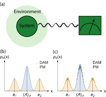
Figure 1: Schematic diagrams. (a) The setup: a dissipative system coupled to a measuring apparatus. The coupling is extremely strong but instantaneous for PMs whereas it is very weak but of long duration for DAMs. (b) An ideal PM corresponds to the strong coupling and short-time limit, with eigenvalues $a_{i}$ of the measured observable $A$ as its outcomes. In contrast, an ideal DAM corresponds to the weak coupling and long-time limit, with the expectation value $\langle A\rangle_{\theta}$ as its outcome. Outcomes from both DAMs and PMs in their ideal cases are still subject to fluctuations (represented by the shaded spread in the plotted probability distribution) originating from position uncertainties in the initial state of the apparatus. (c) In practice, the coupling strength and coupling time are finite, causing some deviations from ideal cases for both PMs and DAMs.

Aided by a simple yet well known model, we show that the QCRB can be beaten by DAMs although it does hold for (ideal) PMs. So, despite the long time requirement in DAMs, their ability of beating the QCRB comes as a surprise and constitutes a significant advancement in our understanding of quantum metrology. Indeed, the outcomes of DAMs are directly connected to some parameter of interest whereas this is never the case for PMs. Such a direct connection allows to extract the value of the parameter from the outcomes in a straightforward manner, in principle without any fundamental limitation on precision. To solve the conflict between our results and the QCRB, we resort to Ref. Seveso et al. (2017) which shows that the QCRB relies on a previously overlooked assumption. This assumption can be severely violated by DAMs. Our work therefore provides an intriguing measurement scheme that can surpass the so-called “ultimate precision” limit.

Apart from being of fundamental interest, our results are important from an application perspective as well. On one hand, DAMs allow for detecting steady states without perturbing them. This somewhat exotic feature could be highly useful in dissipative quantum information processing Plenio et al. (1999); Diehl et al. (2008); Verstraete et al. (2009); Weimer et al. (2010); Kastoryano et al. (2011); Cho et al. (2011); Krauter et al. (2011); Barreiro et al. (2011); Vollbrecht et al. (2011); Kastoryano et al. (2013); Carr and Saffman (2013); Torre et al. (2013); Rao and Mølmer (2013); Bentley et al. (2014); Zhang et al. (2016a, b); Abdi et al. (2016); Kimchi-Schwartz et al. (2016); Reiter et al. (2016); Žnidarič (2016); Reiter et al. (2017), where steady states are typically entangled states or some other desirable states. On the other hand, as shown below, decoherence and dissipation play an integral part in DAMs. As a consequence, if the effects of decoherence and dissipation become increasingly strong, the efficiency of DAMs would increase instead of declining. This theoretical view, verified by numerical simulations below, suggests the fascinating possibility that decoherence and dissipation may be exploited for good rather than causing detrimental effects in quantum measurements.

II preliminaries

We start with some preliminaries. Given a family of quantum states $\rho_{\theta}$ characterized by an unknown parameter $\theta$, a basic task in quantum metrology is to estimate $\theta$ as precisely as possible by using $N$ repeated measurements. Any measurement can be described by a positive operator-valued measure (POVM) $\Pi_{x}$ satisfying $\int dx\ \Pi_{x}=\openone$, with $x$ labeling its outcome. To obtain an estimate of $\theta$, one can input the outcomes $x_{1},\cdots,x_{N}$ of $N$ measurements into an estimator $\hat{\theta}(x_{1},\cdots,x_{N})$, which is a map from the set of outcomes to the parameter space. Upon optimizing over all unbiased estimators for a given measurement, one reaches the classical Cramér-Rao bound (CCRB) $\textrm{Var}(\hat{\theta})\geq[NF(\theta)]^{-1}$. Here $\textrm{Var}(\hat{\theta})$ is the variance of $\hat{\theta}$ and $F(\theta)=\int dxp_{\theta}(x)[\partial_{\theta}\ln p_{\theta}(x)]^{2}$ is the classical Fisher information (CFI), with $p_{\theta}(x)=\mathrm{tr}(\Pi_{x}\rho_{\theta})$ denoting the conditional probability density of getting outcome $x$ when the actual value of the parameter is $\theta$. To find the best precision, one needs to further optimize the CFI $F(\theta)$ over all possible measurements $\Pi_{x}$. In doing this, it has been implicitly assumed that $\Pi_{x}$ is independent of $\theta$ Braunstein and Caves (1994); Paris (2009); Helstrom (1967). Under this assumption, referred to as the $\theta$-independence assumption hereafter, one can prove that $F(\theta)\leq H(\theta)$, with $H(\theta)=\mathrm{tr}(\rho_{\theta}L_{\theta}^{2})$ denoting the QFI expressed in terms of the symmetric logarithmic derivative $L_{\theta}$, i.e., the Hermitian operator satisfying $\partial_{\theta}\rho_{\theta}=\frac{1}{2}(L_{\theta}\rho_{\theta}+\rho_{\theta}L_{\theta})$. Substituting $F(\theta)\leq H(\theta)$ into the CCRB, one arrives at the QCRB $\textrm{Var}(\hat{\theta})\geq[NH(\theta)]^{-1}$. As the $\theta$-independence assumption has never been doubted until the recent work Seveso et al. (2017), it has been believed for a long time that the QCRB is universally valid for all kinds of measurements and, therefore, represents the ultimate precision allowed by quantum mechanics. Moreover, the optimal POVM (asymptotically) saturating this bound has been shown to be the PM associated with the observable $A_{\textrm{opt}}=\theta\openone+L_{\theta}/H(\theta)$ Paris (2009). The proof of the QCRB is revisited in Appendix A. Shortly, we will show that DAMs violate the $\theta$-independence assumption and can be exploited to beat the QCRB.

To better digest the above knowledge, we may take the generalized amplitude damping process Nielsen and Chuang (2010) as an example. It is described by the Lindblad equation, $\frac{d}{dt}\rho(t)=\mathcal{L}_{\theta}\rho(t)$, where $\mathcal{L}_{\theta}\rho:=\gamma[\theta(\sigma_{-}\rho\sigma_{+}-\frac{1}{2}\{\sigma_{+}\sigma_{-},\rho\})+(1-\theta)(\sigma_{+}\rho\sigma_{-}-\frac{1}{2}\{\sigma_{-}\sigma_{+},\rho\})]$ is a Liouvillian superoperator depending on the parameter $\theta\in(0,1)$, with $\gamma$ denoting the decay rate, $\sigma_{-}=|0\rangle\langle 1|$, and $\sigma_{+}=|1\rangle\langle 0|$. For this dissipative process, there is a unique steady state $\rho_{\theta}=\textrm{diag}(\theta,1-\theta)$, which can be approached if the evolution time is much longer than the relaxation time of the process. Our purpose here is to infer the value of $\theta$ from $N$ repeated measurements on $\rho_{\theta}$. Considering that $\theta$ is a monotone function of the temperature of environment Nielsen and Chuang (2010), estimation of $\theta$ offers one means of temperature estimation that has received much attention recently in quantum thermometry Mancino et al. (2017); Mehboudi et al. (2019); Seah et al. (2019). Using $\rho_{\theta}=\textrm{diag}(\theta,1-\theta)$, we have $L_{\theta}=\textrm{diag}(\frac{1}{\theta},-\frac{1}{1-\theta})$ and further obtain $H(\theta)=\frac{1}{\theta(1-\theta)}$. So, the QCRB reads $\textrm{Var}(\hat{\theta})\geq\theta(1-\theta)/N$. On the other hand, direct calculations show that $A_{\textrm{opt}}=|0\rangle\langle 0|$. Clearly, the PM associated with $A_{\textrm{opt}}$ has two potential outcomes $1$ and $0$, with the probabilities $\theta$ and $1-\theta$, respectively. Intuitively, one may think of $1$ and $0$ as the head and tail of a coin, with $\theta$ corresponding to the coin’s propensity to land heads. Performing $N$ such PMs, we can obtain a series of data, $x_{1}^{\textrm{PM}},\cdots,x_{N}^{\textrm{PM}}$, with $x_{i}^{\textrm{PM}}\in\{1,0\}$. Then the value of $\theta$ can be estimated as, $\hat{\theta}(x_{1}^{\textrm{PM}},\cdots,x_{N}^{\textrm{PM}}):=\sum_{i=1}^{N}x_{i}^{\textrm{PM}}/N$, amounting to the frequency of $1$ appearing in the data. Using well known results regarding $N$-trial coin flip experiments, we have

$$\textrm{Var}(\hat{\theta})=\theta(1-\theta)/N,$$ (1)

indicating that the PM associated with $A_{\textrm{opt}}$ already reaches the QCRB. In passing, given the same amount of resources, e.g., the number of measurements, one may wonder whether the estimation error can be further reduced, e.g., by measuring a (possibly entangled) state other than $\rho_{\theta}$. In Appendix B, we prove that the answer is negative if the QCRB is valid. In order to simplify our paper as much as we can, throughout this paper, we use the above simple example to demonstrate our findings, although our findings are generally applicable to dissipative systems.

III Dissipative adiabatic measurement

Keeping this example in mind, we proceed to develop DAMs. Suppose that we are given a dissipative system $\mathscr{S}$ with a Liouvillian superoperator $\mathcal{L}_{\theta}$. Here we take $\theta$ to be a single parameter for simplicity. $\mathcal{L}_{\theta}$ is assumed to be such that: (a) it admits a unique steady state $\rho_{\theta}$; (b) the nonzero eigenvalues $\lambda_{h}$ ($h>0$) of $\mathcal{L}_{\theta}$ have negative real parts, that is, there is a dissipative gap $\Delta:=\min_{h>0}\lvert\textrm{Re}(\lambda_{h})\rvert$ in the Liouvillian spectrum. $\mathscr{S}$ is initially prepared in its steady state $\rho_{\theta}$. Note that this is achievable even though $\theta$ is unknown, as $\mathscr{S}$ automatically approaches $\rho_{\theta}$ because of the dissipative gap Plenio et al. (1999); Diehl et al. (2008); Verstraete et al. (2009); Weimer et al. (2010); Kastoryano et al. (2011); Cho et al. (2011); Krauter et al. (2011); Barreiro et al. (2011); Vollbrecht et al. (2011); Kastoryano et al. (2013); Carr and Saffman (2013); Torre et al. (2013); Rao and Mølmer (2013); Bentley et al. (2014); Zhang et al. (2016a, b); Abdi et al. (2016); Kimchi-Schwartz et al. (2016); Reiter et al. (2016); Žnidarič (2016); Reiter et al. (2017). To simplify our discussion, we adopt the minimal model of measurement that has been used time and again in the literature (see Appendix C for more details). That is, to measure an observable $A$, we add an interaction term, $H_{I}=T^{-1}A\otimes\hat{p}$, coupling $\mathscr{S}$ to a measuring apparatus $\mathscr{A}$, with coordinate and momentum denoted by $\hat{x}$ and $\hat{p}$, respectively. Here, $T$ is a positive real number, which, in the spirit of the adiabatic theorem, will be eventually sent to infinity Aharonov and Vaidman (1993). As usual, we are not interested in the dynamics of the apparatus itself and assume its free Hamiltonian to be zero Aharonov and Vaidman (1993). In real situations, this could be achieved by switching to a rotating frame. The dynamics of the coupling procedure is described by the equation ($\hbar=1$),

$$\frac{d}{dt}\rho(t)=\mathcal{L}_{\theta}\rho(t)-i\left[H_{I},\rho(t)\right]=:\mathcal{L}\rho(t).$$ (2)

If the coupling time is $T$ (so that the product of the coupling strength, i.e., $1/T$, and the coupling time is unity), $\mathscr{S}+\mathscr{A}$ undergoes the dynamical map, $\mathcal{E}_{T}:=e^{\mathcal{L}T}$, transforming the initial state $\rho_{\theta}\otimes|\phi\rangle\langle\phi|$ to the state $\mathcal{E}_{T}(\rho_{\theta}\otimes|\phi\rangle\langle\phi|)$ at time $T$. Here, $|\phi\rangle$ denotes the initial state of $\mathscr{A}$, which is set to be a Gaussian centered at $x=0$. After the coupling procedure, the coordinate $\hat{x}$ is observed, in order to determine the reading of the pointer. The above minimal model can be implemented in a number of experimental setups, such as in cavity quantum electrodynamics Hood et al. (2000); Mabuchi and Doherty (2002) and circuit quantum electrodynamics Blais et al. (2004); Wallraff et al. (2004).

To figure out the effect of $\mathcal{E}_{T}$, we make use of the fact $\mathcal{L}(\rho\otimes|p\rangle\langle p^{\prime}|)=(\mathcal{L}_{p,p^{\prime}}\rho)\otimes|p\rangle\langle p^{\prime}|$, with $\mathcal{L}_{p,p^{\prime}}\rho:=\mathcal{L}_{\theta}\rho-iT^{-1}(pA\rho-p^{\prime}\rho A)$. Here, $|p\rangle$ denotes the eigenstate of $\hat{p}$, i.e., $\hat{p}|p\rangle=p|p\rangle$. This leads to $\mathcal{E}_{T}(\rho_{\theta}\otimes|p\rangle\langle p^{\prime}|)=(e^{\mathcal{L}_{p,p^{\prime}}T}\rho_{\theta})\otimes|p\rangle\langle p^{\prime}|$. Note that a technical result in Ref. Zanardi and Venuti (2014) is

$$\lVert e^{\mathcal{L}_{p,p^{\prime}}T}\mathcal{P}_{\theta}-e^{\widetilde{\mathcal{L}}_{p,p^{\prime}}T}\mathcal{P}_{\theta}\rVert=O(1/T),$$ (3)

indicating that $e^{\mathcal{L}_{p,p^{\prime}}T}\mathcal{P}_{\theta}$ gets closer and closer to $e^{\widetilde{\mathcal{L}}_{p,p^{\prime}}T}\mathcal{P}_{\theta}$ as $T$ approaches infinity 1no . Here, $\widetilde{\mathcal{L}}_{p,p^{\prime}}:=\mathcal{P}_{\theta}\mathcal{L}_{p,p^{\prime}}\mathcal{P}_{\theta}$, and $\mathcal{P}_{\theta}$ denotes the projection, $\mathcal{P}_{\theta}(X):=(\mathrm{tr}_{\mathscr{S}}X)\rho_{\theta}$, mapping an arbitrary operator $X$ into $\rho_{\theta}$. Using Eq. (3) and noting that the explicit expression of $\widetilde{\mathcal{L}}_{p,p^{\prime}}$ reads $\widetilde{\mathcal{L}}_{p,p^{\prime}}=-iT^{-1}(p-p^{\prime})\langle A\rangle_{\theta}\mathcal{P}_{\theta}$, where $\langle A\rangle_{\theta}:=\mathrm{tr}(A\rho_{\theta})$, we obtain

$$\lim_{T\rightarrow\infty}\mathcal{E}_{T}(\rho_{\theta}\otimes|p\rangle\langle p^{\prime}|)=\rho_{\theta}\otimes e^{-i(p-p^{\prime})\langle A\rangle_{\theta}}|p\rangle\langle p^{\prime}|.$$ (4)

Now, expressing $|\phi\rangle$ in $\mathcal{E}_{T}(\rho_{\theta}\otimes|\phi\rangle\langle\phi|)$ as $|\phi\rangle=\int\phi(p)|p\rangle dp$ and using the linearity of the map $\mathcal{E}_{T}$ as well as Eq. (4), we arrive at the main formula of this paper,

$$\lim_{T\rightarrow\infty}\mathcal{E}_{T}(\rho_{\theta}\otimes|\phi\rangle\langle\phi|)=\rho_{\theta}\otimes e^{-i\langle A\rangle_{\theta}\hat{p}}|\phi\rangle\langle\phi|e^{i\langle A\rangle_{\theta}\hat{p}}.$$ (5)

Formula (5) shows that in the weak coupling and long time limit, the steady state $\rho_{\theta}$ does not collapse and the pointer is shifted by the expectation value rather than eigenvalues of $A$ (see Fig. 1b).

To gain physical insight into the above result, we compare DAMs with PMs. Both DAMs and PMs utilize interaction terms of the form, $H_{I}=g(t)A\otimes\hat{p}$, with $g(t)$ normalized to $\int g(t)dt=1$. Note that we have let $g(t)=1/T$ for simplicity. In PMs, this term is impulsive, that is, $g(t)=1/T$ takes an extremely large value but only for a very short time interval. So, the dominating term in Eq. (2) is $H_{I}$. In the strong coupling and short time limit, i.e., $T\rightarrow 0$, the associated dynamical map reads

$$\lim_{T\rightarrow 0}\mathcal{E}_{T}(\rho_{\theta}\otimes|\phi\rangle\langle\phi|)=e^{-iA\otimes\hat{p}}\rho_{\theta}\otimes|\phi\rangle\langle\phi|e^{iA\otimes\hat{p}}.$$ (6)

Clearly, this map creates correlations between $\mathscr{S}$ and $\mathscr{A}$, giving rise to the quantum back action that the configuration of $\mathscr{S}$ after the measurement is determined by the outcome of $\mathscr{A}$. Contrary to PMs, DAMs exploit the opposite limit of an extremely weak but long time interaction, i.e., $T\rightarrow\infty$. For this, the dissipative term $\mathcal{L}_{\theta}$ dominates the interaction term $H_{I}$ in Eq. (2). The former effectively eliminates correlations created by the latter through continuously projecting $\mathscr{S}$ into its steady state $\rho_{\theta}$. Resulted from this nontrivial interplay is the decoupling of $\mathscr{S}$ and $\mathscr{A}$ in the long time limit, which inhibits the state of $\mathscr{S}$ from any change or collapse. Such a mechanism is suggestive of the quantum Zeno effect, making DAMs distinct from PMs in nature.

Now let us turn to the practical situation with the coupling strength and the coupling time being finite. In a PM, under the influence of $\mathcal{L}_{\theta}$, i.e., decoherence and dissipation, the evolved state $\mathcal{E}_{T}(\rho_{\theta}\otimes|\phi\rangle\langle\phi|)$ deviates from the ideal correlated state given by Eq. (6). To ensure that such deviations are small enough, it has to be required that $H_{I}$ is sufficiently strong so that decoherence and dissipation are comparatively weak. Evidently, such a strong interaction requirement would be increasingly difficult to meet if decoherence and dissipation become increasingly strong. This is consistent with our intuition that decoherence and dissipation are detrimental in quantum measurements. Contrary to this understanding, DAMs appreciate decoherence and dissipation as useful resources because they are responsible for eliminating the system-apparatus correlations. Certainly, in a non-ideal DAM due to a finite $T$, the evolved state also deviates from the ideal decoupled state in Eq. (5) (see Fig. 1c). Nevertheless, the stronger decoherence and dissipation are, the more efficient the correlation elimination is and, therefore, the shorter the coupling time required to execute a DAM. That is, unlike the strong interaction requirement in PMs, the long time requirement in DAMs would be increasingly easy to meet if decoherence and dissipation are increasingly strong. This point can be placed on more solid ground by virtue of perturbation theory Zhang and Gong .

To illustrate the above point, we come back to the foregoing example. Here, $\gamma$ represents the strength of decoherence and dissipation; more precisely, the dissipative gap $\Delta=\gamma/2$. Note that the deviations in PM and DAM from their ideal results can be quantified by the measures

$$\lVert\mathcal{E}_{T}(\rho_{\theta}\otimes|\phi\rangle\langle\phi|)-\lim_{T\rightarrow 0}\mathcal{E}_{T}(\rho_{\theta}\otimes|\phi\rangle\langle\phi|)\rVert$$ (7)

and

$$\lVert\mathcal{E}_{T}(\rho_{\theta}\otimes|\phi\rangle\langle\phi|)-\lim_{T\rightarrow\infty}\mathcal{E}_{T}(\rho_{\theta}\otimes|\phi\rangle\langle\phi|)\rVert,$$ (8)

respectively.

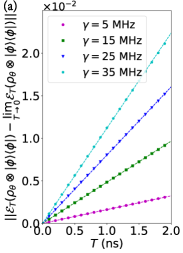
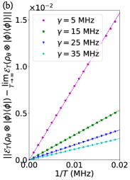
Figure 2: Numerical results of the measures in Eqs. (7) and (8) for (a) PM and (b) DAM with different $\gamma$.

Figure 2 shows these two measures for different $\gamma$, where we set, without loss of generality, $A=A_{\textrm{opt}}=|0\rangle\langle 0|$, $\theta=1/2$, and $\sigma=1/5$, with $\sigma$ denoting the standard deviation of the Gaussian $|\phi\rangle$. The characteristic scales of the physical quantities used in Fig. 2 are chosen with a realistic model in mind Hatridge et al. (2013). As can be easily seen from Fig. 2, the slope of Eq. (7) as a function of $T$ increases as $\gamma$ increases. This indicates that $1/T$ has to be increasingly large in PM for achieving a certain desired tolerance of the deviations. In contrast, as shown in Fig. 2, the slope of Eq. (8) as a function of $1/T$ decreases as $\gamma$ increases, implying that $T$ can be increasingly small in DAM for achieving the same tolerance. For instance, if the desired tolerance is set to be 0.01, $1/T$ in PM are 162, 483, 802, 1119 MHz whereas $T$ in DAM are 78.7, 26.6, 16.0, 11.5 $\mu$s, for $\gamma=5,15,25,35$ MHz, respectively. More numerical results revealing effects arising from an intermediate coupling time are presented in Appendix D. Besides, we have examined one of the experimental setups Hatridge et al. (2013) used to implement the minimal model of measurement adopted here and obtained analogous results (see Appendix E).

IV Beating the Quantum Cramér-Rao Bound

Having proposed DAMs, we now show that they can beat the QCRB. Imagine that the PM used in the foregoing example is replaced by the DAM associated with $A_{\textrm{opt}}=|0\rangle\langle 0|$. Analogous to $N$ PMs, $N$ such DAMs produce a series of data, $x_{i}^{\textrm{DAM}}$, $i=1,\cdots,N$, where $x_{i}^{\textrm{DAM}}$ denotes the outcome of the $i$th DAM. As before, these data can be further input into the estimator, $\hat{\theta}(x_{1}^{\textrm{DAM}},\cdots,x_{N}^{\textrm{DAM}})=\sum_{i=1}^{N}x_{i}^{\textrm{DAM}}/N$, to obtain an estimate of $\theta$. Note that the probability density of getting $x_{i}^{\textrm{DAM}}$ in the (ideal) DAM is

$$p_{\theta}(x_{i}^{\textrm{DAM}})=\frac{1}{\sqrt{2\pi\sigma^{2}}}e^{-\frac{(x_{i}^{\textrm{DAM}}-\theta)^{2}}{2\sigma^{2}}},$$ (9)

which can be verified by using Eq. (5) and noting that $\langle A_{\textrm{opt}}\rangle_{\theta}=\theta$ (see Appendix F). It follows that $\hat{\theta}(x_{1}^{\textrm{DAM}},\cdots,x_{N}^{\textrm{DAM}})$ is an unbiased estimator with

$$\textrm{Var}(\hat{\theta})=\sigma^{2}/N.$$ (10)

For the sake of comparing Eq. (10) with Eq. (1), we stress that Eq. (1) is, strictly speaking, obtained under the limiting condition that the PM is ideal and $\sigma\rightarrow 0$. Indeed, the probability density of getting $x_{i}^{\textrm{PM}}$ in the (ideal) PM is (see Appendix F)

$$p_{\theta}(x_{i}^{\textrm{PM}})=\frac{\theta}{\sqrt{2\pi\sigma^{2}}}e^{-\frac{(x_{i}^{\textrm{PM}}-1)^{2}}{2\sigma^{2}}}+\frac{1-\theta}{\sqrt{2\pi\sigma^{2}}}e^{-\frac{{x_{i}^{\textrm{PM}}}^{2}}{2\sigma^{2}}}.$$ (11)

Equation (11) is, as a matter of fact, a continuous probability distribution but can be treated as the discrete probability distribution giving rise to Eq. (1) in the limit of $\sigma\rightarrow 0$ (see Appendix F). In contrast to Eq. (1), $\textrm{Var}(\hat{\theta})$ in Eq. (10) approaches zero as $\sigma\rightarrow 0$, indicating that there is no fundamental limitation on precision in the DAM. Here we point out that $\textrm{Var}(\hat{\theta})$ in Eq. (10) is, as a matter of fact, limited by the the standard deviation of the normal distribution (9), but this is not a fundamental limitation but a limitation stemming from non-ideal experimental conditions. Furthermore, it can be shown that the POVM operator associated with the DAM is $\Pi_{x^{\textrm{DAM}}}=\frac{1}{\sqrt{2\pi\sigma^{2}}}e^{-\frac{(x^{\textrm{DAM}}-\theta)^{2}}{2\sigma^{2}}}\openone$ (see Appendix F). Evidently, it violates the $\theta$-independence assumption, which is the technical reason for the DAM to be able to beat the QCRB.

Lastly, it may be instructive to give a simple physical picture for comprehending the result that the QCRB can be beaten by the DAM. To do this, suppose that we are given only one data, $x_{i}^{\textrm{PM}}$ or $x_{i}^{\textrm{DAM}}$. Roughly speaking, $x_{i}^{\textrm{PM}}$ is either $1$ or $0$, which is unrelated to $\theta$. Thus, there is no way for us to accurately infer $\theta$ from $x_{i}^{\textrm{PM}}$. However, for a small $\sigma$, $x_{i}^{\textrm{DAM}}$ takes a value equal to or close to $\langle A_{\textrm{opt}}\rangle_{\theta}=\theta$, which is directly related to $\theta$. Based on this direct relationship, one can obtain a fairly good estimate from $x_{i}^{\textrm{DAM}}$. In this sense, $x_{i}^{\textrm{DAM}}$ is more informative than $x_{i}^{\textrm{PM}}$. To further confirm this point, one can work out their CFI. The CFI associated with Eq. (9) reads $F^{\textrm{DAM}}(\theta)=1/\sigma^{2}$, whereas that associated with Eq. (11) satisfies $F^{\textrm{PM}}(\theta)\leq H(\theta)$, no matter how small $\sigma$ is (see Appendix F). That is, $F^{\textrm{PM}}(\theta)$ is bounded by the QFI but $F^{\textrm{DAM}}(\theta)$ is unbounded in principle.

V Concluding remarks

Before concluding, we make a few remarks. Equation (10) is nothing but the CCRB for the normal distribution (9). Our finding here is that the CCRB (10) can be infinitely small in principle and, in particular, can be smaller than the QCRB (1). This clearly demonstrates that there is no intrinsic limitation on precision, which is contrary to the quantum Cramér-Rao theorem Braunstein and Caves (1994); Paris (2009). On the other hand, the steady state in our example is a classical state and, therefore, does not display any coherent nature. We emphasize that the reason of choosing this example is due to its simplicity. Our measurement is certainly capable of revealing coherent nature of a quantum system as long as the steady state in question is genuinely quantum. Any system studied in Refs. Verstraete et al. (2009); Kastoryano et al. (2011); Cho et al. (2011); Krauter et al. (2011); Carr and Saffman (2013); Torre et al. (2013); Rao and Mølmer (2013); Bentley et al. (2014); Abdi et al. (2016); Kimchi-Schwartz et al. (2016); Reiter et al. (2016); Žnidarič (2016), as far as we can see, may serve as one illustrative example.

In conclusion, we have proposed an innovative measurement tailored for strongly dissipative systems. In our measurement, the dissipative dynamics continuously eliminates correlations created by the weak system-apparatus interaction, resulting in the decoupling of the system from the apparatus in the long time limit. Unlike PMs, our measurement therefore does not collapse the measured state, and moreover, its outcome is the expectation value of an observable in the steady state, which is directly connected to the parameter of interest. By virtue of this, our measurement is able to beat the QCRB, without suffering from any fundamental limitation on precision. These findings, solidified by a simple but delightful example, provide a revolutionary insight into quantum metrology. We highlight that our measurement works in a state-protective fashion and embraces decoherence and dissipation as useful resources. Such exotic features could be highly useful in dissipative quantum information processing.

Appendix A Revisiting the proof of the QCRB

Here, focusing on the single-parameter case, we revisit the proof of the QCRB Helstrom (1967); Braunstein and Caves (1994); Paris (2009). Suppose that one is given many copies of a quantum state $\rho_{\theta}$ characterized by an unknown parameter $\theta$, and wishes to estimate $\theta$ as precisely as possible by using $N$ repeated measurements. In general, a quantum measurement can be described by a POVM $\{\Pi_{x}\}$. Here, $\Pi_{x}$ is a positive-semidefinite operator satisfying $\int dx\Pi_{x}=\openone$, with $\openone$ denoting the identity operator. $x$ labels the “results” of the measurement. Although written here as a single continuous real variable, $x$ can be discrete or multivariate. Accordingly, the outcomes of $N$ repeated measurements can be expressed as $x_{1},x_{2},\cdots,x_{N}$. In order to extract the value of $\theta$ from these data, one can resort to an estimator, $\hat{\theta}(x_{1},\cdots,x_{N})$, which is a map from the data $x_{1},\cdots,x_{N}$ to the parameter space.

Given a set of outcomes $x_{1},\cdots,x_{N}$, one can obtain an estimate $\hat{\theta}(x_{1},\cdots,x_{N})$ of $\theta$. The deviation of the estimate from the true value of $\theta$ can be quantified by Braunstein and Caves (1994)

$$\delta\theta(x_{1},\cdots,x_{N}):=\frac{\hat{\theta}(x_{1},\cdots,x_{N})}{\lvert d\langle\hat{\theta}\rangle/d\theta\rvert}-\theta.$$ (1)

Here, $\langle\hat{\theta}\rangle$ denotes the statistical average of $\hat{\theta}(x_{1},\cdots,x_{N})$ over potential outcomes $x_{1},\cdots,x_{N}$,

$$\langle\hat{\theta}\rangle=\int dx_{1}\cdots dx_{N}\,p_{\theta}(x_{1})\cdots p_{\theta}(x_{N})\hat{\theta}(x_{1},\cdots,x_{N}),$$

where

$$p_{\theta}(x)=\mathrm{tr}(\Pi_{x}\rho_{\theta}).$$ (3)

The derivative $d\langle\hat{\theta}\rangle/d\theta$ appearing in Eq. (1) is used to remove the local difference in the “units” of the estimate and the parameter Braunstein and Caves (1994). The estimation error can be then defined as Braunstein and Caves (1994)

$${\langle(\delta\theta)^{2}\rangle},$$ (4)

i.e., the statistical average of $\delta\theta^{2}(x_{1},\cdots,x_{N})$ over potential outcomes $x_{1},\cdots,x_{N}$. In particular, if $\hat{\theta}(x_{1},\cdots,x_{N})$ is unbiased, i.e., $\langle\hat{\theta}\rangle=\theta$, there is

$$\delta\theta(x_{1},\cdots,x_{N})=\hat{\theta}(x_{1},\cdots,x_{N})-\langle\hat{\theta}\rangle,$$ (5)

indicating that $\langle(\delta\theta)^{2}\rangle$ is simply the variance adopted in the main text,

$$\langle(\delta\theta)^{2}\rangle={\textrm{Var}(\hat{\theta})},$$ (6)

for an unbiased estimator.

To estimate $\theta$ as precisely as possible, one needs to optimize the estimation error $\langle(\delta\theta)^{2}\rangle$ over all estimators and measurements. This is exactly the way that the QCRB was proven, which can be stated via the following two steps Braunstein and Caves (1994); Paris (2009). The first step is to optimize $\langle(\delta\theta)^{2}\rangle$ over all estimators for a given measurement. This leads to the CCRB,

$$\langle(\delta\theta)^{2}\rangle\geq[{NF(\theta)}]^{-1},$$ (7)

where $F(\theta)$ is the CFI defined as

$$F(\theta) = \int dx\,p_{\theta}(x)\left(\frac{\partial}{\partial\theta}\ln p_{\theta}(x)\right)^{2}$$ (8)

$$= \int dx\,\frac{1}{p_{\theta}(x)}\left(\frac{\partial}{\partial\theta}p_{\theta}(x)\right)^{2}.$$

The CCRB has been widely used in classical estimation theory. Its proof can be found in many articles (e.g., Ref. Braunstein and Caves (1994)) and is definitely correct. We omit it here. The second step is to optimize $F(\theta)$ over all measurements to get the QCRB. This step is based on the following equality Braunstein and Caves (1994); Paris (2009),

$$\frac{\partial}{\partial\theta}p_{\theta}(x)=\mathrm{tr}\left(\Pi_{x}\frac{\partial}{\partial\theta}\rho_{\theta}\right),$$ (9)

which is valid if $\Pi_{x}$ satisfies the $\theta$-independence assumption, as can be seen from Eq. (3).

To get the QCRB from Eq. (9) (see also Ref. Paris (2009)), one needs to introduce the Symmetric Logarithmic Derivative (SLD), which is defined as the Hermitian operator $L_{\theta}$ satisfying

$$\frac{L_{\theta}\rho_{\theta}+\rho_{\theta}L_{\theta}}{2}=\frac{\partial\rho_{\theta}}{\partial\theta}.$$ (10)

Substituting Eq. (10) into Eq. (9) yields

$$\frac{\partial}{\partial\theta}p_{\theta}(x)=\Re[\mathrm{tr}(\rho_{\theta}\Pi_{x}L_{\theta})].$$ (11)

Inserting Eq. (11) into Eq. (8) and using Eq. (3), one has

$$F(\theta)=\int dx\frac{\Re[\mathrm{tr}(\rho_{\theta}\Pi_{x}L_{\theta})]^{2}}{\mathrm{tr}(\Pi_{x}\rho_{\theta})},$$ (12)

which further leads to

$$F(\theta) \leq \int dx\,\lvert\frac{\mathrm{tr}(\rho_{\theta}\Pi_{x}L_{\theta})}{\sqrt{\mathrm{tr}(\Pi_{x}\rho_{\theta})}}\rvert^{2}$$ (13)

$$= \int dx\lvert\mathrm{tr}\left[\frac{\sqrt{\rho_{\theta}}\sqrt{\Pi_{x}}}{\sqrt{\mathrm{tr}(\Pi_{x}\rho_{\theta})}}\sqrt{\Pi_{x}}L_{\theta}\sqrt{\rho_{\theta}}\right]\rvert^{2}.$$

Using the Cauchy-Schwarz inequality $\lvert\mathrm{tr}(X^{\dagger}Y)\rvert^{2}\leq\mathrm{tr}(X^{\dagger}X)\mathrm{tr}(Y^{\dagger}Y)$ for two matrices $X$ and $Y$, one can deduce from Eq. (13) that

$$F(\theta)\leq\int dx\,\mathrm{tr}(\Pi_{x}L_{\theta}\rho_{\theta}L_{\theta})=\mathrm{tr}(L_{\theta}\rho_{\theta}L_{\theta})=\mathrm{tr}(\rho_{\theta}L_{\theta}^{2}).$$

So, the CFI is bounded from above by the so-called QFI

$$F(\theta)\leq H(\theta):=\mathrm{tr}(\rho_{\theta}L_{\theta}^{2}).$$ (15)

Substituting Eq. (15) into Eq. (7), one arrives at the QCRB,

$$\langle(\delta\theta)^{2}\rangle\geq[{NH(\theta)}]^{-1}.$$ (16)

It has never been doubted until recently Seveso et al. (2017) that the QCRB is the ultimate precision allowed by quantum mechanics that cannot be surpassed under any circumstances Braunstein and Caves (1994); Paris (2009). As can be seen from the above proof, Eqs. (15) and (16) as well as this belief are based on the $\theta$-independence assumption. At first glance, this assumption seems reasonable as it echoes with our quick impressions obtained from textbook materials regarding PMs. Indeed, the textbook physics says that the POVM operators associated with a PM are the eigen-projections of the measured observable. An incautious follow-up inference might be that the POVM operators associated with any types of measurements are only determined by the measured observable and, therefore, $\theta$-independent. However, as critically examined below, the POVM operators of a measurement may be determined by many factors in practice, even possibly including the parameter $\theta$ itself. That is, the $\theta$-independence assumption may not be true in practice. Therefore, although the CCRB is always true, the QCRB as a universally valid bound is questionable.

Appendix B Proof of optimality of Eq. (1)

Here, we prove that Eq. (1) is optimal if the QCRB is valid. Let

$$\Lambda_{\theta}(t):=e^{\mathcal{L}_{\theta}t}$$ (17)

be the quantum channel associated with the generalized amplitude damping process. To estimate the parameter $\theta$ characterizing this channel, a general strategy Giovannetti et al. (2006) is to send $N$ probes through $N$ parallel channels $\Lambda_{\theta}(t)$, measure them at the output, and use an inference rule $\hat{\theta}(\bm{x})$ to extract the value of $\theta$ from the measurement results $\bm{x}$ (see Fig. 3).

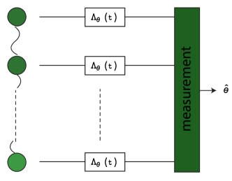
Figure 3: General scheme for quantum metrology. $N$ probes, prepared in an initial state, are sent through $N$ parallel channels $\Lambda_{\theta}(t)$. A measurement is performed on the final state, from which the parameter $\theta$ is estimated via an inference rule $\hat{\theta}$.

Here, we have collectively denoted the measurement outcomes as $\bm{x}$, i.e., $\bm{x}=(x_{1},\cdots,x_{N})$. Therefore, a general scheme of quantum metrology consists of three ingredients: an input state of $N$ probes, a measurement at the output, and an inference rule. In the following, we do not impose any restriction on these ingredients. That is, the input state can be an arbitrary, possibly highly entangled, state; the measurement is a general, not necessarily local, POVM (which is, of course, assumed to be $\theta$-independent so that the QCRB can be applied); and the inference rule can be biased or unbiased. Additionally, $t$ appearing in Eq. (17) can take any non-negative value; it is unnecessary to fulfill the condition assumed in the main text, which requires that the evolution time $t$ is much longer than the relaxation time of the channel.

Using the QCRB Braunstein and Caves (1994), we have that the estimation error is lower bounded by

$$\langle(\delta\theta)^{2}\rangle\geq\frac{1}{{H\left[\Lambda_{\theta}^{\otimes N}(t)[\rho(0)]\right]}}.$$ (18)

Here, $H\left[\Lambda_{\theta}^{\otimes N}(t)[\rho(0)]\right]$ represents the QFI and $\Lambda_{\theta}^{\otimes N}(t)[\rho(0)]$ is the output state of the $N$ probes, where $\rho(0)$ denotes the input state. To evaluate the QFI $H\left[\Lambda_{\theta}^{\otimes N}(t)[\rho(0)]\right]$, we introduce two amplitude damping channels Nielsen and Chuang (2010), $\Lambda_{i}(t)$, $i=0,1$, defined as two completely positive trace-preserving (CPTP) maps transforming the Bloch vector as

$$\Lambda_{0}(t):\ \ (r_{x},r_{y},r_{z})\rightarrow$$

$$(e^{-\frac{\gamma t}{2}}r_{x},e^{-\frac{\gamma t}{2}}r_{y},1-e^{-\gamma t}+e^{-\gamma t}r_{z}),$$ (19)

and

$$\Lambda_{1}(t):\ \ (r_{x},r_{y},r_{z})\rightarrow$$

$$(e^{-\frac{\gamma t}{2}}r_{x},e^{-\frac{\gamma t}{2}}r_{y},e^{-\gamma t}-1+e^{-\gamma t}r_{z}),$$ (20)

respectively. Noting that the effect of $\Lambda_{\theta}(t)$ is

$$\Lambda_{\theta}(t):\ \ (r_{x},r_{y},r_{z})\rightarrow$$

$$\left(e^{-\frac{\gamma t}{2}}r_{x},e^{-\frac{\gamma t}{2}}r_{y},(2\theta-1)(1-e^{-\gamma t})+e^{-\gamma t}r_{z}\right),$$

we have

$$\Lambda_{\theta}(t)=\theta\Lambda_{0}(t)+(1-\theta)\Lambda_{1}(t).$$ (22)

Equation (22) enables us to rewrite $\Lambda_{\theta}(t)$ as a $\theta$-independent quantum channel acting on a larger input space,

$$\Lambda_{\theta}(t)[\rho]=\Phi(t)[\rho\otimes\rho_{\theta}].$$ (23)

Here, $\rho_{\theta}=\textrm{diag}(\theta,1-\theta)$ is the steady state, and $\Phi(t)$ is defined as

$$\Phi(t)[\rho\otimes\sigma] := \sum_{i=0,1}\Lambda_{i}(t)\otimes\mathcal{E}_{i}[\rho\otimes\sigma]$$ (24)

$$= \sum_{i=0,1}\Lambda_{i}(t)[\rho]\otimes\mathcal{E}_{i}[\sigma],$$

where $\mathcal{E}_{i}[\sigma]:=\langle i|\sigma|i\rangle$, $i=0,1$. It is not difficult to see that $\Phi(t)$ thus defined is a CPTP map. Using Eq. (23), we have

$$H\left[\Lambda_{\theta}^{\otimes N}(t)[\rho(0)]\right] = H\left[\Phi^{\otimes N}(t)[\rho(0)\otimes\rho_{\theta}^{\otimes N}]\right]$$ (25)

$$\leq H\left[\rho(0)\otimes\rho_{\theta}^{\otimes N}\right]$$

$$= H\left[\rho_{\theta}^{\otimes N}\right],$$

where we have used the monotonicity of the QFI under parameter-independent CPTP maps Braunstein and Caves (1994). Noting that $H\left[\rho_{\theta}^{\otimes N}\right]=NH\left[\rho_{\theta}\right]$ and $H[\rho_{\theta}]=\frac{1}{\theta(1-\theta)}$, we further have

$$H\left[\Lambda_{\theta}^{\otimes N}(t)[\rho(0)]\right]\leq\frac{N}{\theta(1-\theta)}.$$ (26)

Substituting Eq. (26) into Eq. (18) yields

$$\langle(\delta\theta)^{2}\rangle\geq{\frac{\theta(1-\theta)}{N}},$$ (27)

indicating that Eq. (1) is optimal if the QCRB is valid.

Appendix C More details on the minimal model of quantum measurement

Suppose that $\mathscr{S}$ is a qubit undergoing the generalized amplitude damping process,

$$\frac{d}{dt}\rho_{\mathscr{S}}(t)=\mathcal{L}_{\theta}\rho_{\mathscr{S}}(t),$$ (28)

with $\mathcal{L}_{\theta}$ defined in the main text. Equation (28) can be used to describe the dynamics of a qubit interacting with a Bosonic thermal environment at finite temperature Nielsen and Chuang (2010). In this scenario, $\theta$ is a monotone function of the temperature of the environment, which characterizes losses of energy from the qubit, i.e., effects of energy dissipation Nielsen and Chuang (2010). So, determining $\theta$ amounts to determining the temperature of the environment. Considering that temperature estimation has received much attention recently in quantum thermometry Mancino et al. (2017); Mehboudi et al. (2019); Seah et al. (2019), we aim to estimate $\theta$ in the main text. We assume that the dynamics described by Eq. (28) is always-on. Such an assumption is, of course, reasonable in many physical scenarios/applications, e.g., in quantum computation, where effects of decoherence and dissipation are always-on whenever one implements unitary gates or performs quantum measurements on qubits.

To simplify our discussion here as well as in the main text, we adopt the minimal model of quantum measurement, which has been used time and again in the literature Naghiloo . That is, to measure an observable $A$, we add an interaction term,

$$H_{I}=T^{-1}A\otimes\hat{p},$$ (29)

coupling $\mathscr{S}$ to a measuring apparatus $\mathscr{A}$. Here and in the main text, we have suppressed the subscript $x$ in $\hat{p}$ for ease of notation. The initial state $|\phi\rangle$ of $\mathscr{A}$ is set to be a Gaussian centered at $x=0$,

$$|\phi\rangle=\int dx\frac{1}{(2\pi\sigma^{2})^{1/4}}e^{-\frac{x^{2}}{4\sigma^{2}}}|x\rangle,$$ (30)

where $\sigma$ denotes the standard deviation. Here and henceforth, we omit the two limits of a integral whenever they are $-\infty$ and $+\infty$ for ease of notation. As usual, we are not interested in the free dynamics of $\mathscr{A}$ itself. So, we require the free Hamiltonian of $\mathscr{A}$ to be zero. Such a requirement is often imposed in proposals of quantum measurements and may be satisfied if one goes to a frame that rotates with the free Hamiltonian of $\mathscr{A}$ in the rest frame (see p. 15 of Ref. Naghiloo ). It is worth noting that there are a number of experimental setups (such as in cavity quantum electrodynamics and circuit quantum electrodynamics) that are physically equivalent and therefore can be used to implement the above minimal model Naghiloo . In particular, the above minimal model was also adopted in Aharonov et al.’s proposal of adiabatic measurements Aharonov and Vaidman (1993), which has been experimentally realized in optical setups Piacentini et al. (2017).

It may be helpful to recall a toy setup used to demonstrate the implementation of PM Naghiloo . As schematically shown in Fig. 4,

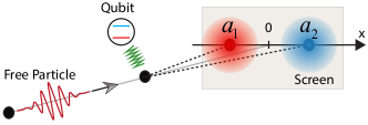
Figure 4: A toy setup used to demonstrate the implementation of PM (see p. 73 of Ref. Naghiloo ). A free particle passes by and interacts with a qubit. The state of the free particle is described by a Gaussian wave packet moving along $z$ direction. Upon interacting with the qubit, the particle is pulled or pushed along $x$ direction, depending on the state of the qubit. In a PM, the position of the particle hitting the screen tells us about the eigenvalues of the measured observable $A$. However, in a DAM, the shift is the expectation value $\langle A\rangle_{\theta}$.

a free particle passing by the qubit plays the role of the measuring apparatus $\mathscr{A}$. Initially, it is prepared in a Gaussian wave packet with a non-zero momentum along $z$ direction,

$$\phi(\bm{r},0)=\frac{1}{(2\pi\sigma^{2})^{3/4}}e^{-\frac{x^{2}+y^{2}+z^{2}}{4\sigma^{2}}}e^{ip_{z}z},$$ (31)

where $p_{z}$ is a fixed positive number describing the $z$-component of the momentum of the particle. Then the wave packet moves along $z$ direction with the group velocity

$$v_{g}=\frac{p_{z}}{m},$$ (32)

where $m$ denotes the mass of the particle. That is,

$$\phi(\bm{r},t)=\frac{1}{(2\pi\sigma^{2})^{3/4}}e^{-\frac{x^{2}+y^{2}+(z-v_{g}t)^{2}}{4\sigma^{2}}}e^{i(p_{z}z-\omega t)},$$ (33)

with $\omega=p_{z}^{2}/(2m)$ ($\hbar=1$). Here, we have neglected the spread of the wave packet by assuming that $m$ is very large. Note that $v_{g}$ can take an arbitrary value because of the freedom in choosing $p_{z}$. Upon interacting with the qubit, the particle gets pulled or pushed along $x$ direction, depending on the state of the qubit. That is, the interaction is of the form $H_{I}=g(t)A\otimes\hat{p}_{x}$. [In Eq. (29), $g(t)$ is assumed to be time-independent for simplicity.] Taking $A=\sigma_{z}$ as an example, we see that whether the particle gets pulled or pushed depends on whether the state of the qubit is $|0\rangle$ or $|1\rangle$. The coupling strength is determined by the distance of the particle from the qubit, whereas the coupling time is determined by the value of $v_{g}$ as well as the distance between the particle and the screen. In a PM, the coupling strength is large and the coupling time is small, so that $H_{I}$ is dominant whereas $\mathcal{L}_{\theta}$ can be neglected. Under the influence of $H_{I}$, the particle hits the screen with some shift along $x$ direction. The shift tells us about an eigenvalue $a_{i}$ of $A$. On the other hand, in a DAM, we consider the scenario that $\mathcal{L}_{\theta}$ is dominant but $H_{I}$ is comparatively weak. The former effectively reshapes the latter to be $g(t)\langle A\rangle_{\theta}\hat{p}_{x}$. So, the shift is now the expectation value $\langle A\rangle_{\theta}$ rather than an eigenvalue $a_{i}$.

According to the minimal model of measurement and noting that the dynamics (28) is always-on, we have that the dynamical equation describing the coupling of $\mathscr{S}$ and $\mathscr{A}$ reads

$$\frac{d}{dt}\rho_{\mathscr{SA}}(t)=\mathcal{L}_{\theta}\rho_{\mathscr{SA}}(t)-i\left[H_{I},\rho_{\mathscr{SA}}(t)\right]=:\mathcal{L}\rho_{\mathscr{SA}}(t).$$

Evidently, the dynamics map associated with the coupling procedure is

$$\mathcal{E}_{T}=e^{\mathcal{L}T},$$ (35)

transforming the initial state $\rho_{\theta}\otimes|\phi\rangle\langle\phi|$ to the state $\mathcal{E}_{T}(\rho_{\theta}\otimes|\phi\rangle\langle\phi|)$ at time $T$. In the main text, we mainly focus on the two limits $T\rightarrow 0$ and $T\rightarrow\infty$, which correspond to PMs and DAMs, respectively. Besides, although $T$ is set to be $\infty$ in DAMs for the sake of mathematical convenience, it is not very large for strongly dissipative systems. Moreover, the larger the dissipative gap is, the shorter $T$ can be. This is analogous to the well known result regarding the adiabatic theorem, where $T$ is determined by the energy gap of the Hamiltonian of a closed system.

Appendix D Discussion on intermediate $T$

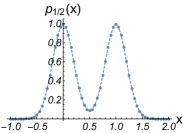
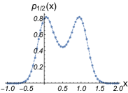
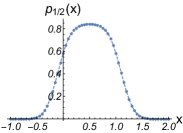
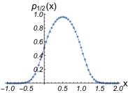
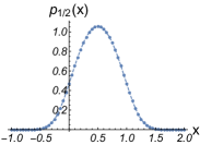
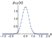
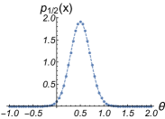
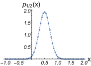
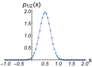
Figure 5: Plots of the probability distribution $p_{1/2}(x)$ for (a) $T=0$ $\mu$s, (b) $T=0.2$ $\mu$s, (c) $T=0.4$ $\mu$s, (d) $T=0.6$ $\mu$s, (e) $T=0.8$ $\mu$s, (f) $T=1$ $\mu$s, (g) $T=10$ $\mu$s, (h) $T=30$ $\mu$s, (i) $T=60$ $\mu$s, and (j) $T=90$ $\mu$s. Parameters used are $\sigma=0.2$ and $\gamma=5$ MHz.

In the main text, we discussed the two limiting cases of $T\rightarrow 0$ and $T\rightarrow\infty$, which correspond to PM and DAM, respectively. The former is the best known type of quantum measurement, which has been extensively studied in the literature. The physical significance of the latter, however, has not been widely appreciated or even fully recognized. The aim of the present work is to study the limiting case of $T\rightarrow\infty$ and show that it is also a novel type of quantum measurement applied to dissipative systems. Here, we would like to go one step further and briefly discuss the case of intermediate $T$, although such a discussion is beyond the focus of this work. To do this, we numerically compute the profile of the probability distribution $p_{\theta}(x)$ for various values of $T$. Some typical examples of the profile are shown in Fig. 5. Here, we choose $\theta=1/2$ without loss of generality. The profile associated with the PM is shown in Fig. 5, in which there are two peaks corresponding to the two eigenvalues $0$ and $1$ of the measured observable $A_{\textrm{opt}}$. As $T$ increases, the probability density at $x=\langle A_{\textrm{opt}}\rangle_{\theta}=1/2$ increases whereas those at $x=0$ and $x=1$ decrease, as shown in Figs. 5-5. This leads to the fact that the two peaks in Fig. 5 finally merge into one peak, as shown in Fig. 5. After that, the probability density at $x=\langle A_{\textrm{opt}}\rangle_{\theta}=1/2$ continues to increase as $T$ increases, so that the peak becomes sharper and sharper, as can be seen from Figs. 5-5. Finally, when $T\geq 30~{}\mu s$, the profile rarely changes even though we continue to enlarge $T$, as can be seen from Figs. 5-5. This indicates that $T=30~{}\mu s$ can be already thought of as being sufficiently large so that the profile now corresponds to the DAM.

Appendix E Discussion on a realistic model

Here we examine the realistic model of a driven superconducting qubit dispersively coupled to a microwave resonator Blais et al. (2004); Wallraff et al. (2004). It is equivalent to the adopted minimal model of measurement and has been used to realize PMs Hatridge et al. (2013). In a frame rotating at the frequency of the driving pulse, the Hamiltonian of the qubit reads $H_{q}=-\frac{\omega_{R0}}{2}(\cos\alpha\sigma_{x}+\sin\alpha\sigma_{y})-\frac{\Delta\omega}{2}\sigma_{z}$, where $\sigma_{i}$, $i=x,y,z$, denote Pauli matrices, and $\omega_{R0}$, $\Delta\omega$, and $\alpha$ are the Rabi frequency, the detuning, and the phase of the driving pulse, respectively Ithier et al. (2005). The qubit is exposed to decoherence and dissipation described by $\mathcal{L}_{d}=\gamma_{1}\mathcal{D}[\sigma_{-}]+\frac{\gamma_{2}}{2}\mathcal{D}[\sigma_{z}]$ with $\mathcal{D}[o]\rho=o\rho o^{\dagger}-\frac{1}{2}\{o^{\dagger}o,\rho\}$, where $\gamma_{i}$, $i=1,2$, are the relaxation and dephasing rates, respectively. The total Liouvillian describing the dynamics of the qubit therefore is $\mathcal{L}_{\textrm{total}}:=-i[H_{q},\bullet]+\mathcal{L}_{d}$, which plays the role of $\mathcal{L}_{\theta}$ in Eq. (C). The interaction between the qubit and the resonator reads $H_{I}=\chi a^{\dagger}a\sigma_{z}$, where $\chi$ represents the dispersive coupling, and $a^{\dagger}$ and $a$ are the creation and annihilation operators for the resonator. The Hamiltonian of the resonator is $H_{r}=\omega_{r}a^{\dagger}a$, where $\omega_{r}$ is the resonator frequency. In PMs, under the influence of $H_{I}$, the frequency of the resonator is shifted as $\omega_{r}\pm\chi$, depending on whether the state of the qubit is $|0\rangle$ or $|1\rangle$. (In DAMs, it should be $\omega_{r}+\chi\langle A\rangle$.) The shift can be read out by coupling the resonator to transmission lines. The average number $\overline{n}$ of photons in the resonator is determined by the power of the readout pulse as well as the decoherence and dissipation experienced by the resonator. Here, we consider the scenario that the decoherence and dissipation of the qubit is much stronger than those of the resonator so that we can neglect the latter within a certain time window. On the other hand, we can suppress the term $H_{r}$ by switching to a rotating frame, that is, we are in a doubly rotating frame. So, we may only consider the two terms $\mathcal{L}_{\textrm{total}}$ and $H_{I}$ as in Eq. (C), in order to figure out the frequency shift resulting from the non-trivial interplay between them. A full analysis taking into account the decoherence and dissipation of the resonator (possibly with experimental demonstration) is left to a future work.

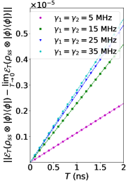
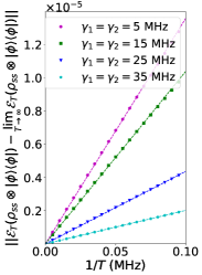
Figure 6: Numerical results of measures (7) and (8) for (a) PM and (b) DAM with different $\gamma_{1}$ and $\gamma_{2}$. Parameters used are: $\omega_{R0}/(2\pi)=2$ MHz, $\alpha=0$, $\Delta\omega=0$, and $\overline{n}=16$.

Figure 6 shows the numerical results of the measures in Eqs. (7) and (8) for different $\gamma_{1}$ and $\gamma_{2}$. Here, we set $\gamma_{1}=\gamma_{2}$ without loss of generality. Also, we identify $\chi$ with $T^{-1}$, for the sake of notational consistency. As can be seen from Fig. 6, as $\gamma_{1}=\gamma_{2}$ increases, the slope of measure (7) as a function of $T$ increases, but that of measure (8) as a function of $1/T$ decreases. This indicates that the strong interaction requirement in PMs is increasingly difficult to meet if decoherence and dissipation become increasingly strong, whereas this is not the case for the long time requirement in DAMs. For instance, if the desired tolerance of the deviations is set to be $10^{-5}$, $1/T$ in PM are 114, 230, 267, 279 MHz whereas $T$ in DAM are 13.6, 10.4, 4.4, 2.0 $\mu$s, for $\gamma_{1}=\gamma_{2}=5,15,25,35$ MHz, respectively. This is consistent with the results found in the main text.

Appendix F Details on examination of the $\theta$-independence assumption

To examine the $\theta$-independence assumption, we need to figure out an expression for the POVM operator $\Pi_{x}$. Noting that the state of $\mathscr{S}+\mathscr{A}$ immediately after the coupling procedure is $\mathcal{E}_{T}(\rho_{\theta}\otimes|\phi\rangle\langle\phi|)$, we have that the probability density of getting the pointer reading $x$ is given by

$$p_{\theta}(x)=\mathrm{tr}_{\mathscr{SA}}\left[|x\rangle\langle x|\mathcal{E}_{T}(\rho_{\theta}\otimes|\phi\rangle\langle\phi|)\right].$$ (36)

Besides, as shown in the main text, there is

$$\mathcal{E}_{T}(\rho_{\theta}\otimes|p\rangle\langle p^{\prime}|)=\left(e^{\mathcal{L}_{p,p^{\prime}}T}\rho_{\theta}\right)\otimes|p\rangle\langle p^{\prime}|,$$ (37)

where

$$\mathcal{L}_{p,p^{\prime}}\rho=\mathcal{L}_{\theta}\rho-iT^{-1}\left(pA\rho-p^{\prime}\rho A\right).$$ (38)

Expressing $|\phi\rangle$ in Eq. (36) as $|\phi\rangle=\int dp\ \phi(p)|p\rangle$ with

$$\phi(p)=\frac{1}{(2\pi\sigma^{\prime 2})^{1/4}}e^{-\frac{p^{2}}{4\sigma^{\prime 2}}}$$ (39)

being the momentum representation of $|\phi\rangle$, where $\sigma^{\prime}=1/(2\sigma)$, we have

$$p_{\theta}(x)=\frac{1}{2\pi}\int dpdp^{\prime}\,\phi(p)\phi^{*}(p^{\prime})e^{i(p-p^{\prime})x}\mathrm{tr}_{\mathscr{S}}\left[e^{\mathcal{L}_{p,p^{\prime}}T}\rho_{\theta}\right].$$

Note that any linear map $\Lambda$ defined over the operator space of $\mathscr{S}$ has a dual map $\Lambda^{*}$, which is the map such that

$$\mathrm{tr}_{\mathscr{S}}[X^{\dagger}\Lambda(Y)]=\mathrm{tr}_{\mathscr{S}}[\Lambda^{*}(X)^{\dagger}Y],$$ (41)

where $X$ and $Y$ are two linear operators acting on the Hilbert space of $\mathscr{S}$. To digest the above definition, one can rewrite Eq. (41) as $\langle X,\Lambda(Y)\rangle=\langle\Lambda^{*}(X),Y\rangle$, where $\langle X,Y\rangle:=\mathrm{tr}_{\mathscr{S}}[X^{\dagger}Y]$ is known as the Hilbert-Schmidt inner product Nielsen and Chuang (2010). So, the dual map $\Lambda^{*}$ of a map $\Lambda$ is defined in a way that is completely analogous to how the Hermitian conjugate $X^{\dagger}$ of a linear operator $X$ is defined. It is not difficult to see that the dual map of $e^{\mathcal{L}_{p,p^{\prime}}T}$ is $e^{\mathcal{L}_{p,p^{\prime}}^{*}T}$ with

$$\mathcal{L}_{p,p^{\prime}}^{*}X=\gamma\left[\theta\left(\sigma_{+}X\sigma_{-}-\frac{1}{2}\{\sigma_{+}\sigma_{-},X\}\right)+(1-\theta)\left(\sigma_{-}X\sigma_{+}-\frac{1}{2}\{\sigma_{-}\sigma_{+},X\}\right)\right]+iT^{-1}\left(pAX-p^{\prime}XA\right).$$ (42)

With the above knowledge, we can rewrite the term $\mathrm{tr}_{\mathscr{S}}[e^{\mathcal{L}_{p,p^{\prime}}T}\rho_{\theta}]$ appearing in Eq. (F) as $\mathrm{tr}_{\mathscr{S}}[(e^{\mathcal{L}_{p,p^{\prime}}^{*}T}I)^{\dagger}\rho_{\theta}]$. From this fact and Eq. (F), it follows that

$$p_{\theta}(x)=\mathrm{tr}_{\mathscr{S}}\left[\frac{1}{2\pi}\int dpdp^{\prime}\,\phi(p)\phi^{*}(p^{\prime})e^{i(p-p^{\prime})x}\left(e^{\mathcal{L}_{p,p^{\prime}}^{*}T}I\right)^{\dagger}\rho_{\theta}\right].$$ (43)

Comparing Eq. (43) with Eq. (3), we arrive at the expression of $\Pi_{x}$,

$$\Pi_{x}=\frac{1}{2\pi}\int dpdp^{\prime}\,\phi(p)\phi^{*}(p^{\prime})e^{i(p-p^{\prime})x}\left(e^{\mathcal{L}_{p,p^{\prime}}^{*}T}I\right)^{\dagger}.$$ (44)

As can be seen from Eq. (42), the term $\mathcal{L}_{p,p^{\prime}}^{*}$ appearing in Eq. (44) is $\theta$-dependent. Hence, it is expected that $\Pi_{x}$ is $\theta$-dependent, too.

To confirm that $\Pi_{x}$ is indeed $\theta$-dependent, let us take a closer look at Eq. (44) in the following. For concreteness, we set the measured observable to be $A_{\textrm{opt}}=|0\rangle\langle 0|$. Using Mathematica, we can find out the explicit expression of $(e^{\mathcal{L}_{p,p^{\prime}}^{*}T}I)^{\dagger}$ appearing in Eq. (44),

$$\left(e^{\mathcal{L}_{p,p^{\prime}}^{*}T}I\right)^{\dagger}=e^{-\left(T\gamma+i\nu\right)/{2}}\begin{pmatrix}\cosh(\mathfrak{S}/{2})+(T\gamma-i\nu)\frac{\sinh(\mathfrak{S}/2)}{\mathfrak{S}}&0\\ 0&\cosh(\mathfrak{S}/{2})+(T\gamma+i\nu)\frac{\sinh(\mathfrak{S}/2)}{\mathfrak{S}}\\ \end{pmatrix},$$ (45)

with

$$\mathfrak{S}=\sqrt{T^{2}\gamma^{2}+2iT\gamma\nu(1-2\theta)-\nu^{2}}.$$ (46)

Here, for ease of notation, we have introduced the new variables

$$\mu=p+p^{\prime},\quad\nu=p-p^{\prime}.$$ (47)

Substituting Eq. (45) into Eq. (44) and noting that $\phi(p)\phi^{*}(p^{\prime})=\frac{1}{(2\pi\sigma^{\prime 2})^{1/2}}\exp[-\frac{\mu^{2}+\nu^{2}}{8\sigma^{\prime 2}}]$ and $d\mu d\nu=2dpdp^{\prime}$, we have

$$\Pi_{x}=\int f(\mu)d\mu\begin{pmatrix}\int g_{1}(\nu)d\nu&0\\ 0&\int g_{2}(\nu)d\nu\\ \end{pmatrix}.$$ (48)

Here,

$$f(\mu) := \frac{1}{4\pi}\frac{1}{(2\pi\sigma^{\prime 2})^{1/2}}\exp\left(-\frac{\mu^{2}}{8\sigma^{\prime 2}}\right),$$ (49)

$$g_{1}(\nu) := \exp\left(-\frac{\nu^{2}}{8\sigma^{\prime 2}}+i\nu x-\frac{T\gamma+i\nu}{2}\right)\times$$ (50)

$$\left[\cosh(\mathfrak{S}/{2})+(T\gamma-i\nu)\frac{\sinh(\mathfrak{S}/2)}{\mathfrak{S}}\right],$$

$$g_{2}(\nu) := \exp\left(-\frac{\nu^{2}}{8\sigma^{\prime 2}}+i\nu x-\frac{T\gamma+i\nu}{2}\right)\times$$ (51)

$$\left[\cosh(\mathfrak{S}/{2})+(T\gamma+i\nu)\frac{\sinh(\mathfrak{S}/2)}{\mathfrak{S}}\right].$$

While it is easy to perform the integration $\int f(\mu)d\mu$, i.e., $\int f(\mu)d\mu=\frac{1}{2\pi}$, it is quite difficult to analytically work out the integration $\int g_{i}(\nu)d\nu$, $i=1,2$, in general. To bypass this difficulty, we consider the two limiting cases of $T\rightarrow 0$ and $T\rightarrow\infty$.

Consider first the limiting case of $T\rightarrow 0$. Using Taylor-series expansions for $g_{1}(\nu)$ and $g_{2}(\nu)$ about $T=0$, we have, up to first order,

$$g_{1}(\nu) = e^{i(x-1)\nu}e^{-\frac{\nu^{2}}{8\sigma^{\prime 2}}}-T\gamma(1-\theta)\times$$ (52)

$$e^{i(x-1)\nu}e^{-\frac{\nu^{2}}{8\sigma^{\prime 2}}}\left[1-\sum_{n=1}^{\infty}\frac{(i\nu)^{n-1}}{n!}\right],$$

and

$$g_{2}(\nu) = e^{ix\nu}e^{-\frac{\nu^{2}}{8\sigma^{\prime 2}}}-T\gamma\theta\times$$ (53)

$$e^{ix\nu}e^{-\frac{\nu^{2}}{8\sigma^{\prime 2}}}\left[1-\sum_{n=1}^{\infty}\frac{(-i\nu)^{n-1}}{n!}\right].$$

Substituting Eqs. (52) and (53) into Eq. (48), we obtain, after some algebra,

$$\Pi_{x}=\Pi_{x}^{(0)}+T\Pi_{x}^{(1)},$$ (54)

with

$$\Pi_{x}^{(0)}=\begin{pmatrix}\frac{1}{\sqrt{2\pi\sigma^{2}}}e^{-\frac{(x-1)^{2}}{2\sigma^{2}}}&0\\ 0&\frac{1}{\sqrt{2\pi\sigma^{2}}}e^{-\frac{x^{2}}{2\sigma^{2}}}\end{pmatrix}$$ (55)

and

$$\Pi_{x}^{(1)}=\begin{pmatrix}-\gamma(1-\theta)\left[\frac{1}{\sqrt{2\pi\sigma^{2}}}e^{-\frac{(x-1)^{2}}{2\sigma^{2}}}-\frac{\textrm{erf}\left(\frac{x}{\sqrt{2}\sigma}\right)-\textrm{erf}\left(\frac{x-1}{\sqrt{2}\sigma}\right)}{2}\right]&0\\ 0&-\gamma\theta\left[\frac{1}{\sqrt{2\pi\sigma^{2}}}e^{-\frac{x^{2}}{2\sigma^{2}}}-\frac{\textrm{erf}\left(\frac{x}{\sqrt{2}\sigma}\right)-\textrm{erf}\left(\frac{x-1}{\sqrt{2}\sigma}\right)}{2}\right]\end{pmatrix}.$$ (56)

Here, $\textrm{erf}(x)$ is known as the Gauss error function, defined as $\textrm{erf}(x)=\frac{1}{\sqrt{\pi}}\int_{-x}^{x}e^{-t^{2}}dt$. Evidently, $\Pi_{x}^{(0)}$ is $\theta$-independent but $\Pi_{x}^{(1)}$ is $\theta$-dependent.

In the limit of $T\rightarrow 0$, which corresponds to the PM, we have that

$$\Pi_{x}=\Pi_{x}^{(0)},$$ (57)

thereby reaching the textbook physics that the POVM operator is $\theta$-independent. This can be understood on an intuitive level. Note that the interaction term $H_{I}$ in Eq. (C) is unrelated to $\theta$, whereas the dissipative term $\mathcal{L}_{\theta}$ is related to $\theta$ and has the effect of making $\Pi_{x}$ $\theta$-dependent. In the limit of $T\rightarrow 0$, the coupling strength is infinitely strong and the coupling time is infinitely short, indicating that $H_{I}$ dominates Eq. (C) whereas $\mathcal{L}_{\theta}$ can be omitted from Eq. (C). As a result, $\Pi_{x}=\Pi_{x}^{(0)}$ is, of course, $\theta$-independent. However, in reality, any interaction is of finite strength and lasts for a finite time interval, implying that $\mathcal{L}_{\theta}$ cannot be completely ignored and plays some role in the measurement. So, in addition to $\Pi_{x}^{(0)}$, the (small) $\theta$-dependent term $T\Pi_{x}^{(1)}$ resulting from the effect of $\mathcal{L}_{\theta}$ appears in Eq. (54). This leads to the fact that $\Pi_{x}$ is $\theta$-dependent in practice. Therefore, strictly speaking, the $\theta$-independence assumption may not hold even for PMs in practice.

What happens if we enlarge $T$? As $H_{I}$ becomes weaker as $T$ increases, $\mathcal{L}_{\theta}$ plays an increasingly important role in the measurement. So, it can be expected that $\Pi_{x}$ depends on $\theta$ increasingly heavily as $T$ increases. Roughly speaking, the degree of the $\theta$-dependence of $\Pi_{x}$ achieves its maximum in the limit of $T\rightarrow\infty$. Motivated by this, we let $T\rightarrow\infty$ in our proposal of measurements and expect that $\Pi_{x}$ depends on $\theta$ so heavily that the QCRB can be beaten by our measurement. This is the basic idea underlying our proposal. By the way, as a matter of fact, the QCRB can be (slightly) beaten even by PMs with small but nonzero $T$, as shown below. Let us now figure out the expression of $\Pi_{x}$ in the limiting case of $T\rightarrow\infty$. It is not difficult to see that

$$g_{1}(\nu)=g_{2}(\nu)=e^{i(x-\theta)\nu}e^{-\frac{\nu^{2}}{8\sigma^{\prime 2}}},$$ (58)

in this limit. Substituting Eq. (58) into Eq. (48), we have

$$\Pi_{x}=\begin{pmatrix}\frac{1}{\sqrt{2\pi\sigma^{2}}}e^{-\frac{(x-\theta)^{2}}{2\sigma^{2}}}&0\\ 0&\frac{1}{\sqrt{2\pi\sigma^{2}}}e^{-\frac{(x-\theta)^{2}}{2\sigma^{2}}}\end{pmatrix},$$ (59)

in the limit of $T\rightarrow\infty$. Evidently, $\Pi_{x}$ in Eq (59) is $\theta$-dependent. As an immediate consequence, the $\theta$-independence assumption does not hold for our proposal of measurements.

F.1 Projective measurement: $T\rightarrow 0$

We now inspect more carefully the limiting case of $T\rightarrow 0$. It corresponds to the case that $H_{I}$ is extremely strong but lasts for a very short time interval, i.e., $H_{I}$ is impulsive. Hereafter, to make our discussion conceptually clear, we refer to the limit of $T\rightarrow 0$ as the impulsive limit. In contrast, the limit of $T\rightarrow\infty$ is referred to as the adiabatic limit hereafter, which corresponds to DAMs to be discussed later on. In the impulsive limit, the probability density of getting the pointer reading $x$ is given by

$$p_{\theta}(x)=\frac{\theta}{\sqrt{2\pi\sigma^{2}}}e^{-\frac{(x-1)^{2}}{2\sigma^{2}}}+\frac{1-\theta}{\sqrt{2\pi\sigma^{2}}}e^{-\frac{x^{2}}{2\sigma^{2}}},$$ (60)

which can be obtained by substituting Eq. (55) into Eq. (3).

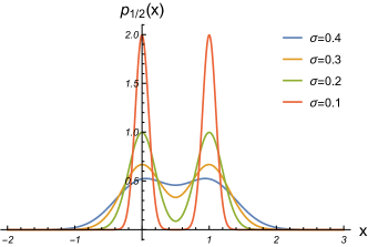
Figure 7: Probability density $p_{1/2}(x)$ of getting the pointer reading $x$ in the impulsive limit with different standard deviations $\sigma$.

For the reader’s information, we plot in Fig. 7 the probability distribution $p_{1/2}(x)$ with different standard deviations $\sigma$. As can be seen from Fig. 7 as well as Eq. (60), for a small $\sigma$, say, $\sigma=0.1$, $p_{\theta}(x)$ is only significantly different from zero if $x\approx 0$ or $x\approx 1$. Noting that $0$ and $1$ are the two eigenvalues of $A_{\textrm{opt}}=|0\rangle\langle 0|$, we deduce that, roughly speaking, the pointer reading $x$, as a random variable, is mostly likely to be one of these two eigenvalues in the PM with a small $\sigma$. This is just the well-known textbook physics that the potential outcome of a PM is one of the eigenvalues of the measured observable. Strictly speaking, this textbook physics is valid only in the mathematical limit of $\sigma\rightarrow 0$, for which the continuous probability distribution $p_{\theta}(x)$ can be treated as a discrete probability distribution. To put it differently, in practice, where $\sigma$ is small but non-zero, the pointer reading $x$ may not be exactly one of the eigenvalues; there could be small fluctuations due to the uncertainty of initial position of the pointer.

It is easy to see that the QFI associated with $\rho_{\theta}$ is given by

$$H(\theta)=\frac{1}{\theta(1-\theta)}.$$ (61)

Equation (61) can be obtained by first solving Eq. (10) to get $L_{\theta}=\textrm{diag}(\frac{1}{\theta},-\frac{1}{1-\theta})$ and then inserting $L_{\theta}$ into Eq. (15). Denote by $F_{\sigma}(\theta)$ the CFI associated with $p_{\theta}(x)$ in Eq. (60). Here, the subscript $\sigma$ is used to indicate that the CFI is dependent of $\theta$ because of the $\theta$-dependence of $p_{\theta}(x)$. Noting that the $\theta$-independence assumption and, therefore, the QCRB holds in the impulsive limit, we have

$$F_{\sigma}(\theta)\leq H(\theta).$$ (62)

On the other hand, it is not difficult to see that

$$\lim_{\sigma\rightarrow 0}F_{\sigma}(\theta)=H(\theta).$$ (63)

Indeed, in the limit of $\sigma\rightarrow 0$, $p_{\theta}(x)$ in Eq. (60) can be treated as the discrete probability distribution with the probability of getting $1$ being $\theta$ and that of getting $0$ being $1-\theta$. Using Eq. (8), one can confirm that the CFI associated with this discrete probability distribution is exactly the QFI given by Eq. (61). Note that the observable corresponding to $p_{\theta}(x)$ in Eq. (60) is $A_{\textrm{opt}}=|0\rangle\langle 0|$. The above point indicates that $A_{\textrm{opt}}=|0\rangle\langle 0|$ is optimal, since the QCRB can be achieved if one performs the PM associated with $A_{\textrm{opt}}$. Combing Eqs. (62) and (63), we have

$$F_{\sigma}(\theta)\leq\lim_{\sigma\rightarrow 0}F_{\sigma}(\theta)=H(\theta).$$ (64)

Figure 8 shows the numerical results of $F_{\sigma}(\theta)$ for four different $\sigma$, namely, $\sigma=0.4,0.3,0.2,0.1$.

Figure 8: Numerical results of the classical Fisher information $F_{\sigma}(\theta)$ associated with $p_{\theta}(x)$ in Eq. (60) for four different $\sigma$. The abscissa and the ordinate are $\theta$ and $1/F_{\sigma}(\theta)$, respectively. The black solid curve represents $1/H(\theta)$. For a given $\theta$, $1/F_{\sigma}(\theta)$ gradually decreases as $\sigma$ decreases and finally approaches the limiting position specified by $1/H(\theta)$ in the limit of $\sigma\rightarrow 0$.

As can be seen from Fig. 8, $1/{F_{\sigma}(\theta)}$ is strictly larger than $1/{H(\theta)}$ for $\sigma>0$ but approximately equals to $1/{H(\theta)}$ for a small enough $\sigma$, say, $\sigma=0.2$. Therefore, to achieve the QCRB, in addition to choosing an optimal observable, one needs to prepare the measuring apparatus $\mathscr{A}$ in a state with a small $\sigma$.

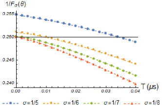
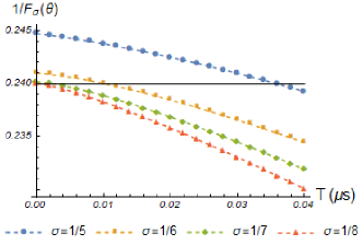
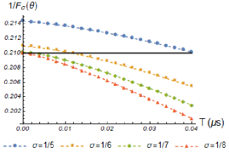
Figure 9: Numerical results of $1/{F_{\sigma}(\theta)}$ with small values of $T$ for three different $\theta$ and four different $\sigma$. (a) $\theta=0.5$. (b) $\theta=0.4$. (c) $\theta=0.3$. The three black solid lines in Figs. 9-9 represent the quantum Cramér-Rao bounds $1/{H(\theta)}$ associated with these three $\theta$, respectively. Here, $\gamma$ is set to be $5$ MHz.

Consider now the PM with a small but nonzero $T$, for which the $\theta$-independence assumption does not hold. Substituting Eq. (54) into Eq. (3), we have that the probability density of getting the pointer reading $x$ is given by

$$p_{\theta}(x)=\frac{\theta-T\gamma\theta(1-\theta)}{\sqrt{2\pi\sigma^{2}}}e^{-\frac{(x-1)^{2}}{2\sigma^{2}}}+\frac{1-\theta-T\gamma\theta(1-\theta)}{\sqrt{2\pi\sigma^{2}}}\times$$

$$e^{-\frac{x^{2}}{2\sigma^{2}}}+T\gamma\theta(1-\theta)\left[\textrm{erf}(\frac{x}{\sqrt{2}\sigma})-\textrm{erf}(\frac{x-1}{\sqrt{2}\sigma})\right].$$ (65)

To examine whether the QCRB can be beaten in this case, we numerically compute $1/{F_{\sigma}(\theta)}$ associated with the $p_{\theta}(x)$ in Eq. (F.1) for three different $\theta$ and four different $\sigma$, namely, $\theta=0.5,0.4,0.3$ and $\sigma=1/5,1/6,1/7,1/8$. The numerical results are shown in Fig. 9, where we set $\gamma=5$ MHz. The three black solid lines depicted in Figs. 9-9 represent the QCRBs $1/{H(\theta)}$ associated with these three values of $\theta$, respectively. As can be seen from Fig. 9, $1/{F_{\sigma}(\theta)}$ can be strictly less than $1/{H(\theta)}$ for some small but nonzero $T$, indicating that the QCRB can be beaten for the PM with a small but nonzero $T$, as claimed in the previous paragraph.

F.2 Dissipative adiabatic measurement: $T\rightarrow\infty$

Consider now the adiabatic limit. In this limit, the probability density of getting outcome $x$ reads

$$p_{\theta}(x)=\frac{1}{\sqrt{2\pi\sigma^{2}}}e^{-\frac{(x-\theta)^{2}}{2\sigma^{2}}},$$ (66)

which can be obtained by substituting Eq. (59) into Eq. (3). For the reader’s information, we plot in Fig. 10 the probability distribution $p_{1/2}(x)$ with different standard deviations $\sigma$.

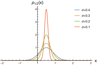
Figure 10: Probability density $p_{1/2}(x)$ of getting the pointer reading $x$ in the adiabatic limit with different standard deviations $\sigma$.

As can be seen from Fig. 10 as well as Eq. (66), for a small $\sigma$, say, $\sigma=0.1$, $p_{\theta}(x)$ is only significantly different from zero if $x\approx\theta$. Note that $\theta$ is the expectation value of $A_{\textrm{opt}}$ in the state $\rho_{\theta}$. So, roughly speaking, the outcome of the DAM is the expectation value of the measured observable, which is in sharp contrast to that of the PM, i.e., an individual eigenvalue of the measured observable.

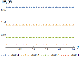
Figure 11: Classical Fisher information $F_{\sigma}(\theta)$ associated with $p_{\theta}(x)$ in Eq. (66) for four different $\sigma$. The abscissa and the ordinate are $\theta$ and $1/{F_{\sigma}(\theta)}$, respectively. For a given $\theta$, $1/{F_{\sigma}(\theta)}$ decreases as $\sigma$ decreases and finally approaches zero in the limit of $\sigma\rightarrow 0$.

Substituting Eq. (66) into Eq. (8), we have that the associated CFI reads

$$F_{\sigma}(\theta)=\frac{1}{\sigma^{2}}.$$ (67)

Figure 11 shows the profiles of $1/{F_{\sigma}(\theta)}$ for four different $\sigma$. As can be easily seen from Eq. (67) as well as Fig. 11, $F_{\sigma}(\theta)$ can be arbitrarily large so long as $\sigma$ is small enough. Therefore, there is no intrinsic bound on precision in the DAM, in sharp contrast to the ideal PM case (see Fig. 8). To better digest this point, one may proceed as follows. Suppose that we are only given one data, which is obtained from the measurement associated with $A_{\textrm{opt}}=|0\rangle\langle 0|$. If the measurement is a PM, this data, denoted as $x^{\textrm{PM}}$, is either $1$ or $0$, provided that $\sigma$ is very small. Evidently, the data $x^{\textrm{PM}}$ itself is unrelated to the parameter $\theta$. Therefore, given only one data $x^{\textrm{PM}}$, there is no way to definitely determine $\theta$ from $x^{\textrm{PM}}$ even in principle. However, if the measurement is a DAM, this data, denoted as $x^{\textrm{DAM}}$, is approximately equal to $\theta$. So, $x^{\textrm{DAM}}$ is more informative than $x^{\textrm{PM}}$, as $x^{\textrm{DAM}}$ is directly related to $\theta$. Such a direct relationship allows one to extract the value of $\theta$ from $x^{\textrm{DAM}}$ straightforwardly, leading to the fact that $\theta$ can be determined to any degree of accuracy so long as $\sigma$ is small enough.

References

- Seveso et al. (2017) L. Seveso, M. A. C. Rossi, and M. G. A. Paris, Phys. Rev. A 95, 012111 (2017).
- Helstrom (1976) C. W. Helstrom, Quantum Detection and Estimation Theory (Academic, New York, 1976).
- Braunstein and Caves (1994) S. L. Braunstein and C. M. Caves, Phys. Rev. Lett. 72, 3439 (1994).
- Paris (2009) M. G. A. Paris, Int. J. Quantum Inform. 07, 125 (2009).
- Helstrom (1967) C. W. Helstrom, Phys. Lett. 25A, 101 (1967).
- Giovannetti et al. (2004) V. Giovannetti, S. Lloyd, and L. Maccone, Science 306, 1330 (2004).
- Giovannetti et al. (2006) V. Giovannetti, S. Lloyd, and L. Maccone, Phys. Rev. Lett. 96, 010401 (2006).
- Giovannetti et al. (2011) V. Giovannetti, S. Lloyd, and L. Maccone, Nat. Photonics 5, 222 (2011).
- Braun et al. (2018) D. Braun, G. Adesso, F. Benatti, R. Floreanini, U. Marzolino, M. W. Mitchell, and S. Pirandola, Rev. Mod. Phys. 90, 035006 (2018).
- Aharonov and Vaidman (1993) Y. Aharonov and L. Vaidman, Phys. Lett. A 178, 38 (1993).
- Beige et al. (2000) A. Beige, D. Braun, B. Tregenna, and P. L. Knight, Phys. Rev. Lett. 85, 1762 (2000).
- Plenio et al. (1999) M. B. Plenio, S. F. Huelga, A. Beige, and P. L. Knight, Phys. Rev. A 59, 2468 (1999).
- Diehl et al. (2008) S. Diehl, A. Micheli, A. Kantian, B. Kraus, H. P. Büchler, and P. Zoller, Nat. Phys. 4, 878 (2008).
- Verstraete et al. (2009) F. Verstraete, M. M. Wolf, and J. I. Cirac, Nat. Phys. 5, 633 (2009).
- Weimer et al. (2010) H. Weimer, M. Müller, I. Lesanovsky, P. Zoller, and H. P. Büchler, Nat. Phys. 6, 382 (2010).
- Kastoryano et al. (2011) M. J. Kastoryano, F. Reiter, and A. S. Sørensen, Phys. Rev. Lett. 106, 090502 (2011).
- Cho et al. (2011) J. Cho, S. Bose, and M. S. Kim, Phys. Rev. Lett. 106, 020504 (2011).
- Krauter et al. (2011) H. Krauter, C. A. Muschik, K. Jensen, W. Wasilewski, J. M. Petersen, J. I. Cirac, and E. S. Polzik, Phys. Rev. Lett. 107, 080503 (2011).
- Barreiro et al. (2011) J. T. Barreiro, M. Müller, P. Schindler, D. Nigg, T. Monz, M. Chwalla, M. Hennrich, C. F. Roos, P. Zoller, and R. Blatt, Nature (London) 470, 486 (2011).
- Vollbrecht et al. (2011) K. G. H. Vollbrecht, C. A. Muschik, and J. I. Cirac, Phys. Rev. Lett. 107, 120502 (2011).
- Kastoryano et al. (2013) M. J. Kastoryano, M. M. Wolf, and J. Eisert, Phys. Rev. Lett. 110, 110501 (2013).
- Carr and Saffman (2013) A. W. Carr and M. Saffman, Phys. Rev. Lett. 111, 033607 (2013).
- Torre et al. (2013) E. G. D. Torre, J. Otterbach, E. Demler, V. Vuletic, and M. D. Lukin, Phys. Rev. Lett. 110, 120402 (2013).
- Rao and Mølmer (2013) D. D. B. Rao and K. Mølmer, Phys. Rev. Lett. 111, 033606 (2013).
- Bentley et al. (2014) C. D. B. Bentley, A. R. R. Carvalho, D. Kielpinski, and J. J. Hope, Phys. Rev. Lett. 113, 040501 (2014).
- Zhang et al. (2016a) D.-J. Zhang, H.-L. Huang, and D. M. Tong, Phys. Rev. A 93, 012117 (2016a).
- Zhang et al. (2016b) D.-J. Zhang, X.-D. Yu, H.-L. Huang, and D. M. Tong, Phys. Rev. A 94, 052132 (2016b).
- Abdi et al. (2016) M. Abdi, P. Degenfeld-Schonburg, M. Sameti, C. Navarrete-Benlloch, and M. J. Hartmann, Phys. Rev. Lett. 116, 233604 (2016).
- Kimchi-Schwartz et al. (2016) M. E. Kimchi-Schwartz, L. Martin, E. Flurin, C. Aron, M. Kulkarni, H. E. Tureci, and I. Siddiqi, Phys. Rev. Lett. 116, 240503 (2016).
- Reiter et al. (2016) F. Reiter, D. Reeb, and A. S. Sørensen, Phys. Rev. Lett. 117, 040501 (2016).
- Žnidarič (2016) M. Žnidarič, Phys. Rev. Lett. 116, 030403 (2016).
- Reiter et al. (2017) F. Reiter, A. S. Sørensen, P. Zoller, and C. A. Muschik, Nat. Commun. 8, 1822 (2017).
- Nielsen and Chuang (2010) M. A. Nielsen and I. L. Chuang, Quantum Computation and Quantum Information (Cambridge University Press, Cambridge, England, 2010).
- Mancino et al. (2017) L. Mancino, M. Sbroscia, I. Gianani, E. Roccia, and M. Barbieri, Phys. Rev. Lett. 118, 130502 (2017).
- Mehboudi et al. (2019) M. Mehboudi, A. Lampo, C. Charalambous, L. A. Correa, M. Ángel García-March, and M. Lewenstein, Phys. Rev. Lett. 122, 030403 (2019).
- Seah et al. (2019) S. Seah, S. Nimmrichter, D. Grimmer, J. P. Santos, V. Scarani, and G. T. Landi, Phys. Rev. Lett. 123, 180602 (2019).
- Hood et al. (2000) C. J. Hood, T. W. Lynn, A. C. Doherty, A. S. Parkins, and H. J. Kimble, Science 287, 1447 (2000).
- Mabuchi and Doherty (2002) H. Mabuchi and A. C. Doherty, Science 298, 1372 (2002).
- Blais et al. (2004) A. Blais, R.-S. Huang, A. Wallraff, S. M. Girvin, and R. J. Schoelkopf, Phys. Rev. A 69, 062320 (2004).
- Wallraff et al. (2004) A. Wallraff, D. I. Schuster, A. Blais, L. Frunzio, R.-S. Huang, J. Majer, S. Kumar, S. M. Girvin, and R. J. Schoelkopf, Nature 432, 162 (2004).
- Zanardi and Venuti (2014) P. Zanardi and L. C. Venuti, Phys. Rev. Lett. 113, 240406 (2014).
- (42) Unless otherwise stated, the Hilbert-Schmidt norm is adopted. That is, for an operator , the norm reads , while for a superoperator , it is the induced norm defined as .
- (43) D.-J. Zhang and J. Gong, arXiv:1907.10340 .
- Hatridge et al. (2013) M. Hatridge, S. Shankar, M. Mirrahimi, F. Schackert, K. Geerlings, T. Brecht, K. M. Sliwa, B. Abdo, L. Frunzio, S. M. Girvin, R. J. Schoelkopf, and M. H. Devoret, Science 339, 178 (2013).
- (45) M. Naghiloo, arXiv:1904.09291 .
- Piacentini et al. (2017) F. Piacentini, A. Avella, E. Rebufello, R. Lussana, F. Villa, A. Tosi, M. Gramegna, G. Brida, E. Cohen, L. Vaidman, I. P. Degiovanni, and M. Genovese, Nat. Phys. 13, 1191 (2017).
- Ithier et al. (2005) G. Ithier, E. Collin, P. Joyez, P. J. Meeson, D. Vion, D. Esteve, F. Chiarello, A. Shnirman, Y. Makhlin, J. Schriefl, and G. Schön, Phys. Rev. B 72, 134519 (2005).