Multilevel Ensemble Kalman Filtering based on a sample average of independent EnKF estimators

Abstract.

We introduce a new multilevel ensemble Kalman filter method (MLEnKF) which consists of a hierarchy of independent samples of ensemble Kalman filters (EnKF). This new MLEnKF method is fundamentally different from the preexisting method introduced by Hoel, Law and Tempone in 2016, and it is suitable for extensions towards multi-index Monte Carlo based filtering methods. Robust theoretical analysis and supporting numerical examples show that under appropriate regularity assumptions, the MLEnKF method has better complexity than plain vanilla EnKF in the large-ensemble and fine-resolution limits, for weak approximations of quantities of interest. The method is developed for discrete-time filtering problems with finite-dimensional state space and linear observations polluted by additive Gaussian noise.

Key words: Monte Carlo, multilevel, convergence rates, Kalman filter, ensemble Kalman filter.

AMS subject classification: 65C30, 65Y20.

1. Introduction

We develop a new multilevel ensemble Kalman filter method (MLEnKF) for the setting of finite-dimensional state space and discrete-time partial observations polluted by additive Gaussian noise. Our method makes use of recent hierarchical variance-reduction techniques [20, 14, 18] to improve the asymptotic efficiency of weak approximations of filtering distributions compared to standard ensemble Kalman filtering (EnKF). We consider settings where solutions of nonlinear dynamics models must be approximated by numerical methods.

The herein introduced MLEnKF method consists of a hierarchy of independent samples of pairwise-coupled EnKF estimators where, in particular, the Kalman gains of every EnKF sample thus also are independent. Our method is fundamentally different from the “canonical” MLEnKF [22], which consists of a hierarchy of coupled ensembles on different resolution levels, all sharing one global “multilevel” Kalman gain.

The motivations for developing the new MLEnKF method are threefold. First, the method is closer to classic EnKF, and we therefore believe it will be easier to implement for practitioners. Second, imposing slightly stricter regularity assumptions, we can prove better asymptotic efficiency results for this method than for the “canonical” one. And third, creating a rigorous convergence theory for the new MLEnKF method is a stepping stone towards a multi-index Ensemble Kalman filtering (MIEnKF) method; See [19] for highly efficient approximations of McKean–Vlasov dynamics by the multi-index Monte Carlo method, and Appendix D for a sketch of the said extension to MIEnKF.

The main theoretical contributions of this work are Theorems 1 and 2, which respectively derive $L^{p}$-convergence rates for weak approximations in the large-ensemble and fine-numerical-resolution limits with EnKF. Theorem 2 is novel, and while Theorem 1 is similar to [22, Theorem 3.11]; but, to the best of our knowledge, this is the first fully proved convergence result for EnKF in the said limits (i.e., in both limits simultaneously). Estimates for EnKF’s and MLEnKF’s asymptotic computational cost versus accuracy for the respective methods are provided in Corollaries 1 and 2, respectively. From these estimates we conclude that MLEnKF asymptotically outperforms EnKF whenever Assumptions 1 and 2 hold.

1.1. Literature review

The EnKF method was first introduced in the seminal work [12], and due to its ease of use and impressive performance in high dimensions, it quickly became a popular method for weather prediction, ocean-atmosphere science, and oil reservoir simulations [29, 26, 1]. The standard version of EnKF with perturbed observations, which is the method we will study and extend to the multilevel setting in this work, first appeared in [25] and ensuing analysis [6] showed that adding artificial noise to the observations may be viewed as a consistency step for avoiding covariance deflation of the empirical filtering distribution. $L^{p}$-convergence of the first and second sample moments in the large-ensemble limit for EnKF was first treated by a short argument in [37] for the linear model setting and the result was subsequently extended to a set of nonlinear filtering problems by a more technical argument in [36] (in the sense of deriving $L^{p}$-convergence rates for weak approximations of sufficiently smooth quantities of interest).

The multilevel Monte Carlo (MLMC) method was introduced for efficient weak approximations of random fields in [20] and for stochastic differential equations in [14]. The MLEnKF method was developed for finite-dimensional settings in [22] and countable, infinite-dimensional settings in [7]. In [13] a multilevel hybrid EnKF method was developed for solving reservoir history matching problems. Multilevel particle filters using a multilevel-coupled resampling algorithm was introduced in [27]. The multilevel transform particle filter, applying optimal transportation mapping in the analysis step, was treated in [17, 16]. In the context of Bayesian inverse problems, multilevel sequential Monte Carlo methods have been studied in [3, 2, 38, 34] and a multilevel Markov Chain Monte Carlo method was developed in [10]. The multi-fidelity Monte Carlo method [39] is a recent and close kin of MLMC that differs from MLMC by having fixied its estimator’s finest resolution level and by having more extensive coupling of samples than only pairwise. This often reduces the estimator’s statistical error even more effectively than MLMC. A multi-fidelity Monte Carlo EnKF method was developed in [40].

Under sufficient regularity, EnKF converges to the so-called mean-field Kalman filter in the large-ensemble limit. In nonlinear-dynamics or observation settings, however, the mean-field Kalman filter is not equal to the Bayes filter [35, 36, 11, 41]. Due to this discrepancy between EnKF and the Bayes filter even in the large-ensemble limit, due to the large uncertainty in the estimation of the model error and due to the constraints imposed by challening high-dimensional problems and limited computational budgets, a considerable number of works have, instead of studying the large-ensemble limit, focused on the large-time and/or continuous-time limit of the fixed-ensemble-size EnKF cf. [30, 46, 42, 43, 5, 9, 33]. However, a recurring problem for fixed-ensemble-size EnKF is to determine how large the ensemble ought to be to equilibrate the model error with the other error contributions (statistical error and bias). And the large-ensemble limit convergence rates for EnKF and MLEnKF that are presented in this work may be helpful for determining the ensemble size of a finite-ensemble EnKF method.

1.2. Organization of this work

Section 2 describes the problem, the MLEnKF method, and $L^{p}$-convergence results for EnKF and MLEnKF towards the mean-field EnKF. Section 3 presents numerical performance studies of EnKF and MLEnKF for two different problems. Appendix A presents a brief overview of the mean-field EnKF method. Appendix B contains proofs of the main theoretical results, Appendix C describes an algorithm for obtaining pseudo-reference solutions for nonlinear filtering problems, and Appendix D sketches an extension from MLEnKF to multi-index EnKF.

2. Problem setting and main results

2.1. Problem setting

Let $(\Omega,(\mathcal{F}_{t}),\mathcal{F}=\mathcal{F}_{\infty},\mathbb{P})$ denote a complete filtered probability space, and for any $k\in\mathbb{N}$ and $p\geq 1$, let $L^{p}_{t}(\Omega,\mathbb{R}^{k})$ denote the space of $\mathcal{F}_{t}\backslash\mathcal{B}^{k}-$measurable functions $u:\Omega\to\mathbb{R}^{k}$ such that $\mathbb{E}\left[|u|^{p}\right]<\infty$. Here, $\mathcal{B}^{k}$ represents the Borel $\sigma$-algebra on $\mathbb{R}^{k}$ and $u$ is said to be $\mathcal{F}_{t}\backslash\mathcal{B}^{k}-$measurable if and only if $u^{-1}(B)\in\mathcal{F}_{t}$ for all $B\in\mathcal{B}^{k}$. For a given state-space dimension $d\in\mathbb{N}$ and initial data $u_{0}\in\cap_{p\geq 2}L^{p}_{0}(\Omega,\mathbb{R}^{d})$, we consider the discrete stochastic dynamics for $n=0,1,\ldots$

(1) $$u_{n+1}(\omega)=\Psi_{n}(u_{n},\omega),\qquad\omega\in\Omega,$$

for a sequence of mappings $\Psi_{n}:\mathbb{R}^{d}\times\Omega\to\mathbb{R}^{d}$. The dynamics is associated with the stochastic differential equation (SDE)

(2) $$\Psi_{n}(u_{n},\omega)=u_{n}+\int_{n}^{n+1}a(u_{t})dt+\int_{n}^{n+1}b(u_{t})dW_{t}(\omega),$$

with coefficients $a:\mathbb{R}^{d}\to\mathbb{R}^{d}$, $b:\mathbb{R}^{d}\to\mathbb{R}^{d\times d_{W}}$ and the driving noise $W:[0,\infty)\times\Omega\to\mathbb{R}^{d_{W}}$ denoting a $d_{W}$-dimensional standard Wiener process. We further assume the coefficients $a$ and $b$ are sufficiently smooth so that

$$u_{n}\in L_{n}^{2}(\Omega,\mathbb{R}^{d})\implies u_{n+1}\in L^{2}_{n+1}(\Omega,\mathbb{R}^{d}),$$

and we note, from now on suppressing the dependence on $\omega$ whenever confusion is not possible, that $u_{n+1}$ may be expressed as a quasi-iterated mapping of $u_{0}$:

$$u_{n+1}=\Psi_{n}\circ\Psi_{n-1}\circ\cdots\circ\Psi_{0}(u_{0}).$$

Associated with the dynamics (1), there exists a series of noisy observations

(3) $$y_{n}=Hu_{n}+\eta_{n},\quad n=1,2,\ldots,$$

where $H\in\mathbb{R}^{d_{O}\times d}$ and $\eta_{1},\eta_{2},\ldots$ is a sequence of independent and identically distributed (iid) random variables satisfying $\eta_{1}\sim N(0,\Gamma)$ with positive definite covariance matrix $\Gamma\in\mathbb{R}^{d_{O}\times d_{O}}$ and the independence property $\{\eta_{j}\}_{j\geq 1}\perp\{u_{k}\}_{k\geq 0}$. The filtration $\mathcal{F}_{t}$ is the completion of the smallest $\sigma$-algebra generated by $u_{0}$, $\{W_{s}\}_{s\in[0,t]}$ and $\{\eta_{j}\}_{j=1}^{\lfloor t\rfloor}$, with $\lfloor t\rfloor=\max\{k\in\mathbb{Z}\mid k\leq t\}$. That is,

$$\mathcal{F}_{t}=\overline{\sigma\Big{(}\sigma(u_{0})\cup\sigma(\{W_{s}\}_{s\in[0,t]})\cup\sigma(\{\eta_{j}\}_{j=1}^{\lfloor t\rfloor})\Big{)}}.$$

with $\overline{\sigma}$ denoting the completion of $\sigma$.

The series of observations up to time $k$ is denoted by

(4) $$Y_{k}:=\begin{cases}(y_{1},y_{2},\ldots,y_{k})&\text{if}\quad k\geq 1,\\ \emptyset&\text{if}\quad k=0.\end{cases}$$

For notational convenicence and since no observations have been made at time $0$, we defined $Y_{0}=\emptyset$ above. In consistency with the propery that $Y_{0}$ holds no information we write $\mathbb{P}_{u_{0}\mid Y_{0}}:=\mathbb{P}_{u_{0}}$. The Bayes filter is a sequential procedure for determining the (conditional) prediction $\mathbb{P}_{u_{k}\mid Y_{k-1}}$ and update $\mathbb{P}_{u_{k}\mid Y_{k}}$. Assuming that the densities of said distributions exist, the stochastic dynamics (1) and the conditional independence $(u_{k}|u_{k-1})\perp Y_{k-1}$ yield the proportionality

$$\begin{split}\rho_{u_{k}\mid Y_{k-1}}(u)&=\int_{\mathbb{R}^{d}}\rho_{u_{k},u_{k-1}\mid Y_{k-1}}(u,v)dv\propto\int_{\mathbb{R}^{d}}\rho_{u_{k}\mid u_{k-1}}(u)\rho_{u_{k-1}\mid Y_{k-1}}(v)\,dv,\end{split}$$

and Bayesian inference implies that

$$\begin{split}\rho_{u_{k}\mid Y_{k}}(u)&\propto\mathcal{L}_{u_{k}|y_{k}}(u)\rho_{u_{k}\mid Y_{k-1}}(u),\end{split}$$

where the likelihood function is given by

$$\mathcal{L}_{u_{k}|y_{k}}(u)=\frac{\exp(-|\Gamma^{-1/2}(y_{k}-Hu)|^{2}/2)}{\sqrt{(2\pi)^{p}|\mathrm{det}(\Gamma)}|}.$$

In other words, if the updated distribution $\mathbb{P}_{u_{k-1}\mid y_{k-1}}$ is known and suitable regularity assumptions hold, then the prediction and updated distribution at the next time can be computed up to a proportionality constant (although this step may be computationally intractable).

In settings where $u_{0}$ is a Gaussian random variable and the dynamics $\Psi$ is linear with additive Gaussian noise, the Kalman filter [28] solves the above filtering problem exactly. When $\Psi$ is nonlinear, however, it is often not possible to solve the filtering problem exactly and one must resort to approximation methods. EnKF is a nonlinear and ensemble-based filtering method that preserves that tends to be particularly efficient when the “true” dimension of a filtering problem is far smaller than the state-space dimension.

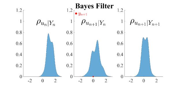
For linear-Gaussian filtering problems, the empirical measure of EnKF converges towards the exact (Bayes filter) density $\mathbb{P}_{u_{k}\mid Y_{k}}$ in the large-ensemble limit [37]. More generally, for instance when $\Psi$ is nonlinear, EnKF converges to the mean-field EnKF in the large-ensemble limit, cf. Section A. As a consequence of EnKF employing a Gaussian-like update of its particles, the mean-field EnKF will in many cases not be equal to the Bayes filter [35, 11]. But, to the best of our knowledge, there does not exist any thorough scientific comparison of the mean-field EnKF and the Bayes Filter, and Figure 1 shows that for the nonlinear dynamics $\Psi$ defined by the SDE

(5) $$du=-(u+\pi\cos(\pi u/5)/5)dt+\sigma dW$$

and (1), the dissipative/contractive properties of the associated Fokker-Planck equation can produce prediction densities for the respective filtering methods that are indistinguishable to the naked eye.

Figure 1. Illustration, based on the nonlinear dynamics (5), of the contracting property which can produce almost identical prediction densities (middle panels) for the Bayes filter and MFEnKF even when the preceding updated densities differ notably.

Objective

For a given quantity of interest (QoI) $\varphi:\mathbb{R}^{d}\to\mathbb{R}$, our objective is to construct an efficient filtering method for computing

(6) $$\mathbb{E}^{\bar{\mu}_{n}}[\varphi(u)]=\int_{\mathbb{R}^{d}}\varphi(u)\bar{\mu}_{n}(du),$$

where $\bar{\mu}_{n}$ denotes the mean-field EnKF updated measure at time $n$, cf. Appendix A. In the best of worlds, one would rather seek a method computing the exact expectation of $\varphi$ with respect to the Bayes filter posterior, i.e., $\mathbb{E}\left[\varphi(u_{n})\mid Y_{n}\right]$, but since the said posterior $\mathbb{P}_{u_{n}\mid Y_{n}}$ is generally not attainable by EnKF-based filtering methods, and since both EnKF and MLEnKF converge weakly towards mean-field EnKF, cf. Theorems 1 and 2, we will in this work focus on the simpler (but still very challenging) goal (6).

Notation 1.

• For $f,g:(0,\infty)\to[0,\infty)$ the notation $f\lesssim g$ implies there exists a $C>0$ such that

  $$f(x)\leq Cg(x),\quad\forall x\in(0,\infty).$$

• The notation $f\eqsim g$ implies that $f\lesssim g$ and $g\lesssim f$.

• For $r,s\in\mathbb{N}$, $|x|$ denotes the Euclidean norm of a vector $x\in\mathbb{R}^{s}$ and for $A\in\mathbb{R}^{r\times s}$, $|A|_{2}:=\sup_{|x|=1}|Ax|$.

• For $\mathcal{F}\backslash\mathcal{B}^{d}$-measurable functions $u:\Omega\to\mathbb{R}^{d}$ and $p\geq 1$,

  $$\left\|u\right\|_{p}:=\left\|u\right\|_{L^{p}(\Omega,\mathbb{R}^{d})}=\left(\int_{\Omega}|u(\omega)|^{p}\,\mathbb{P}(d\omega)\right)^{1/p}.$$

• For any $\kappa\in\mathbb{N}_{0}^{r}$, with $\mathbb{N}_{0}:=\mathbb{N}\cup\{0\}$, and any sufficiently smooth functions of the form $f:\mathbb{R}^{r}\to\mathbb{R}$ and $g:\mathbb{R}^{r}\times\Omega\to\mathbb{R}$, the respective $\partial^{\kappa}$-partial derivatives are defined by

  $$\partial^{\kappa}f(x)=\frac{\partial^{\left|\kappa\right|_{1}}f}{\partial x_{1}^{\kappa_{1}}\ldots\partial x_{r}^{\kappa_{d}}}(x)\quad\text{and}\quad\partial^{\kappa}g(x,\omega)=\frac{\partial^{\left|\kappa\right|_{1}}g}{\partial x_{1}^{\kappa_{1}}\ldots\partial x_{r}^{\kappa_{d}}}(x,\omega)$$

  for all $x\in\mathbb{R}^{r}$ and $\mathbb{P}-$almost all $\omega\in\Omega$, where $|\kappa|_{1}:=\sum_{i=1}^{r}\kappa_{i}$. This extends to vector-valued mappings of the form $f:\mathbb{R}^{r}\to\mathbb{R}^{s}$ by component-wise partial derivatives: $\partial^{\kappa}f(x)=(\partial^{\kappa}f_{1}(x),\partial^{\kappa}f_{2}(x),\ldots,\partial^{\kappa}f_{s}(x))$, and so on.

• For $k\in\mathbb{N}_{0}$, $C^{k}_{B}(\mathbb{R}^{r},\mathbb{R}^{s})$ denotes the space of $k$-times continuously differentiable functions $\eta:\mathbb{R}^{r}\to\mathbb{R}^{s}$ for which $\eta$ and all of its partial derivatives of order up to and including $k$ is uniformly bounded.

• $C^{k}_{P}(\mathbb{R}^{r},\mathbb{R}^{s})$ denotes the space of $k$-times continuously differentiable functions whose partial derivatives of order up to and including $k$ have polynomial growth.

• For a mapping $\eta:\mathbb{R}^{r}\to\mathbb{R}^{s}$, its Jacobian is denoted $D\eta$, and its Hessian is $D^{2}\eta$.

• $\mathbb{R}_{r}[x_{1},\ldots,x_{d}]$ denotes the set of polynomials in $d$ variables that are of total degree smaller or equal to $r\in\mathbb{N}_{0}$ and have coefficients in $\mathbb{R}$.

2.2. Numerical approximation of the stochastic dynamics

We assume that for every time $n\geq 0$, there exists a collection of progressively more accurate numerical solvers $\{\Psi^{N}_{n}:\mathbb{R}^{d}\times\Omega\to\mathbb{R}^{d}\}_{N\in\mathbb{N}}$ satisfying the following assumptions:

Assumption 1.

The initial distribution $u_{0}\in\cap_{p\geq 2}L^{p}_{0}(\Omega,\mathbb{R}^{d})$ and for any $n\in\mathbb{N}_{0}$,

• for any $p\geq 2$, there exists a $c_{p}>0$ such that

  $$\left\|\Psi^{N}_{n}(u)\right\|_{p}\leq c_{p}(1+\left\|u\right\|_{p})\quad\;\forall\big{(}N\in\mathbb{N}\quad\&\quad u\in\cap_{p\geq 2}L^{p}_{n}(\Omega,\mathbb{R}^{d})\,\big{)}\,;$$

• there exists an $\alpha>0$ and a set of mappings $\mathbb{F}$ with $\mathbb{R}_{2}[x_{1},\ldots,x_{d}]\subset\mathbb{F}\subset C^{2}_{P}(\mathbb{R}^{d},\mathbb{R})$ such that if

  $$\begin{split}\left|\mathbb{E}\left[\varphi(u^{N})-\varphi(u)\right]\right|\leq c_{\varphi}N^{-\alpha}\quad\;\forall(N\geq 1\quad\&\quad\varphi\in\mathbb{F}),\end{split}$$

  for some $u\in\cap_{p\geq 2}L^{p}_{n}(\Omega,\mathbb{R}^{d})$ and $\{u^{N}\}_{N}\subset\cap_{p\geq 2}L^{p}_{n}(\Omega,\mathbb{R}^{d})$ and (observable-dependent constant) $c_{\varphi}>0$, then there exists another (observable-dependent constant) $\tilde{c}_{\varphi}>0$ such that

  $$\left|\mathbb{E}\left[\varphi(\Psi^{N}_{n}(u^{N}))-\varphi(\Psi_{n}(u))\right]\right|\leq\tilde{c}_{\varphi}N^{-\alpha}\quad\forall(N\geq 1\quad\&\quad\varphi\in\mathbb{F})\,;$$

• for any $p\geq 2$, there exists a $c_{p}>0$ such that

  $$\left\|\Psi^{N}_{n}(u)-\Psi^{N}_{n}(v)\right\|_{p}<c_{p}\left\|u-v\right\|_{p}\quad\;\forall\big{(}N\in\mathbb{N}\quad\&\quad u,v\in\cap_{p\geq 2}L^{p}_{n}(\Omega,\mathbb{R}^{d})\,\big{)};$$

• there exists a $c_{3}>0$ such that the computational cost of the numerical solution $\Psi^{N}_{n}$ is $\mathbb{P}$-almost surely bounded by

  $$\mathrm{Cost}(\Psi^{N}_{n}(u))\leq c_{3}N\quad\;\forall\big{(}N\in\mathbb{N}\quad\&\quad u\in\cap_{p\geq 2}L^{p}_{n}(\Omega,\mathbb{R}^{d})\,\big{)};$$

Remark 1.

If the dynamics (1) is given by the SDE (2) where the coefficients $a:\mathbb{R}^{d}\to\mathbb{R}^{d}$, $b:\mathbb{R}^{d}\to\mathbb{R}^{d\times d_{W}}$ satisfy $\partial^{\kappa}a_{j},\partial^{\kappa}b_{jk}\in C_{B}(\mathbb{R}^{d},\mathbb{R})$ for all $1\leq j\leq d$, $1\leq k\leq d_{W}$ and $|\kappa|\geq 1$, and if $\Psi^{N}_{n}$ denotes the Euler–Maruyama numerical solution of (2) using $N$ uniform timesteps, then Assumption 1 holds with $\alpha=1$ and $\mathbb{F}=C^{4}_{P}(\mathbb{R}^{d},\mathbb{R})$, cf. [15, Chapter 7] and [31, Thm 14.5.2]. Noting that the uniformly-bounded constraint is only imposed on partial derivatives of the coefficients, and not the coefficients themselves, the stated convergence rates for Euler–Maruyama apply for instance to the nonlinear dynamics (5).

2.3. EnKF

For a solver $\Psi^{N}$ with fixed resolution $N\geq 1$ and a fixed ensemble size $P\geq 1$, the EnKF method consists of an ensemble of $P$ particles that are iteratively simulated forward and updated in a way that can be viewed as a nonlinear extension of Kalman filtering. The evolution of the EnKF ensemble over the times $n=0,1,\ldots$ can be described as follows:

We denote the updated ensemble at time $n$ by $\hat{v}_{n,1:P}^{N,P}:=\{\hat{v}_{n,i}^{N,P}\}_{i=1}^{P}$ and the prediction ensemble at the same time by $v_{n,1:P}^{N,P}:=\{v_{n,i}^{N,P}\}_{i=1}^{P}$. At time $0$, $\hat{v}_{0,1:P}^{N,P}:=\{\hat{v}_{0,i}^{N,P}\}_{i=1}^{P}$, consists of $P$ independent and $\mathbb{P}_{u_{0}|Y_{0}}$-distributed particles, where we assume the initial distribution can be sampled exactly. The empirical measure induced by the ensemble $\hat{v}_{0,1:P}^{N,P}$ may be viewed as the EnKF approximation of $\mathbb{P}_{u_{0}|Y_{0}}$. Given an updated ensemble at time $n\geq 0$, the prediction ensemble at time $n+1$ is computed by simulating each particle forward

$$v_{n+1,i}^{N,P}=\Psi^{N}_{n}(\hat{v}_{n,i}^{N,P})\quad\text{for}\quad i=1,2,\ldots,P.$$

Thereafter, the updated ensemble at time $n+1$ is computed through assimilating the new measurement $y_{n+1}$ through the Kalman-filter-like and particle-wise formula

$$\hat{v}_{n+1,i}^{N,P}=(I-K_{n+1}^{N,P}H)v_{n+1,i}^{N,P}+K_{n+1}^{N,P}\tilde{y}_{n+1,i}\quad\text{for}\quad i=1,2,\ldots,P.$$

Here

$$K_{n+1}^{N,P}=C^{N,P}_{n+1}H^{\mathbf{T}}(HC^{N,P}_{n+1}H^{\mathbf{T}}+\Gamma)^{-1}$$

denotes the Kalman gain,

(7) $$\begin{split}C_{n+1}^{N,P}&=\overline{\mathrm{Cov}}[v_{n+1}^{N,P}]:=\sum_{i=1}^{P}\frac{v_{n+1,i}^{N,P}\left(v_{n+1,i}^{N,P}\right)^{\mathbf{T}}}{P}-\sum_{i=1}^{P}\frac{v_{n+1,i}^{N,P}}{P}\left(\sum_{i=1}^{P}\frac{v_{n+1,i}^{N,P}}{P}\right)^{\mathbf{T}}\end{split}$$

denotes the biased sample covariance of the ensemble $\hat{v}_{n,1:P}^{N,P}$,

$$\tilde{y}_{n+1,i}=y_{n+1}+\eta_{n+1,i},\quad\text{for}\quad i=1,2,\ldots,P$$

are iid perturbed observations with $\eta_{n+1,1}\sim N(0,\Gamma)$ and $\eta_{j,i}\perp u_{k}$ for all $j\geq 1$, $k\geq 0$. Perturbed observations were originally introduced in [6] to correct an unwanted covariance-deflation feature in the original formulation of EnKF [12].

We note that for all filtering methods considered in this work, the iteratively augmented observation sequence $y_{1},y_{2},y_{3},\ldots$ is assumed to be given, i.e., non-random. The sources of randomness in the EnKF filter are therefore the driving noise in the dynamics and the perturbed observations. For EnKF with dynamics resolution $N$, randomness thus enter through $\{\Psi_{n}^{N,P}\}_{n}$ and $\{\eta_{n,i}\}_{n,i}$. Observe further that since the particles $\hat{v}_{n,1}^{N,P},\hat{v}_{n,2}^{N,P},\ldots,\hat{v}_{n,P}^{N,P}$ are identically distributed, the distribution of $\hat{v}_{n}^{N,P}$ will depend on the ensemble size $P$ and the model resolution $N$.

If Assumption 1 holds, then Theorem 1 implies that $\hat{v}_{n,1:P}^{N,P}\subset\cap_{p\geq 2}L^{p}_{n}(\Omega,\mathbb{R}^{d})$ for any $P\in\mathbb{N}$, $N\in\mathbb{N}$, and $n\in\mathbb{N}_{0}$. This ensures the existence of the EnKF empirical measure

$$\mu_{n}^{N,P}(dv)=\frac{1}{P}\sum_{i=1}^{P}\delta(dv;\hat{v}_{n,i}^{N,P}),$$

with the Dirac measure

$$\delta(dv;y):=\begin{cases}1&\text{if}\quad y\in dv\\ 0&\text{otherwise}.\end{cases}$$

Notation 2.

The expectation of a QoI $\varphi:\mathbb{R}^{d}\to\mathbb{R}$ with respect to the a probability measure $\mu:\mathcal{B}^{d}\to[0,1]$ is denoted by

$$\mu[\varphi]:=\int_{\mathbb{R}^{d}}\varphi(v)\,\mu(dv).$$

Note that the expectation with respect to the EnKF empirical measure takes the form of a sample average

$$\mu_{n}^{N,P}[\varphi]=\frac{1}{P}\sum_{i=1}^{P}\varphi(\hat{v}_{n,i}^{N,P}),$$

and that $\mu_{n}^{N,P}[\varphi]$ in fact is a random variable since it is a function of the ensemble’s $P$ particles $\hat{v}_{n,i}^{N,P}$ (where $P$ obviously is a finite number). For the mean-field measure $\bar{\mu}_{n}=\mu_{n}^{\infty,\infty}$, on the other hand, $\bar{\mu}_{n}[\varphi]$ is a deterministic value; this is a consequence of $P=\infty$.

2.4. MLEnKF

The MLEnKF estimator that we introduce in this work is a sample average of pairwise coupled EnKF estimators $\{\mu_{n}^{N_{\ell},P_{\ell}}[\varphi]\}_{\ell=0}^{L}$ on a hierarchy of resolution levels $\{N_{\ell}\}_{\ell=0}^{L}\subset\mathbb{N}$ and ensemble-size levels $\{P_{\ell}\}_{\ell=0}^{L}\subset\mathbb{N}$. Here, $L$ refers to the finest resolution level of the MLEnKF estimator, and we impose the following exponential-growth constraints on the resolution and ensemble-size sequences:

$$P_{\ell+1}=2P_{\ell}\quad\text{and}\quad N_{\ell}\eqsim 2^{s\ell}\quad\text{for some }s>0.$$

Before writing the explicit form of the MLEnKF estimator, note that since our goal, the value we want to approximate, is deterministic, cf. Notation 2, the following equality holds

$$\bar{\mu}_{n}[\varphi]=\mu_{n}^{\infty,\infty}[\phi]=\mathbb{E}\left[\mu_{n}^{\infty,\infty}[\phi]\right].$$

This motivates the approximation

$$\bar{\mu}_{n}[\varphi]\approx\mathbb{E}\left[\mu_{n}^{N_{L},P_{L}}[\phi]\right]=\mathbb{E}\left[\mu_{n}^{N_{0},P_{0}}[\varphi]\right]+\sum_{\ell=1}^{L}\mathbb{E}\left[\mu_{n}^{N_{\ell},P_{\ell}}[\varphi]-\mu_{n}^{N_{\ell-1},P_{\ell-1}}[\varphi]\right],$$

where the last equality holds due to the linearity of the expectation operator. In the expectations for $\ell\geq 1$ we seek to employ pairwise coupling between the fine-level estimator $\mu_{n}^{N_{\ell},P_{\ell}}[\varphi]$ and the coarse-level estimator $\mu_{n}^{N_{\ell-1},P_{\ell-1}}[\varphi]$ through associating the driving noise and perturbed observations for each particle on level $\ell$ uniquely to one particle on level $\ell-1$. As the number of particles on the neighboring levels are not equal ($P_{\ell}=2P_{\ell-1}$), this is clearly not possible in the current form of expectations of differences, so we replace $\mu_{n}^{N_{\ell-1},P_{\ell-1}}[\varphi]$ by the average of two identically distributed random variables $\mu_{n}^{N_{\ell-1},P_{\ell-1},1}[\varphi]$ and $\mu_{n}^{N_{\ell-1},P_{\ell-1},2}[\varphi]$. Importantly, these satisfy

$$\mathbb{E}\left[\frac{\mu_{n}^{N_{\ell-1},P_{\ell-1},1}[\varphi]+\mu_{n}^{N_{\ell-1},P_{\ell-1},2}[\varphi]}{2}\right]=\mathbb{E}\left[\mu_{n}^{N_{\ell-1},P_{\ell-1}}[\varphi]\right]\quad k=1,2,$$

which implies that the following equality holds

$$\begin{split}\mathbb{E}\left[\mu_{n}^{N_{L},P_{L}}[\phi]\right]=&\mathbb{E}\left[\mu_{n}^{N_{0},P_{0}}[\varphi]\right]+\sum_{\ell=1}^{L}\mathbb{E}\left[\mu_{n}^{N_{\ell},P_{\ell}}[\varphi]-\frac{\mu_{n}^{N_{\ell-1},P_{\ell-1},1}[\varphi]+\mu_{n}^{N_{\ell-1},P_{\ell-1},2}[\varphi]}{2}\right].\end{split}$$

By approximating the $\ell$-th the expectation by a sample average using $M_{\ell}$ iid pairwise-coupled samples

$$\left\{\mu_{n}^{N_{\ell},P_{\ell},m}[\varphi]-\frac{\mu_{n}^{N_{\ell-1},P_{\ell-1},1,m}[\varphi]+\mu_{n}^{N_{\ell-1},P_{\ell-1},2,m}[\varphi]}{2}\right\}_{m=1}^{M_{\ell}},$$

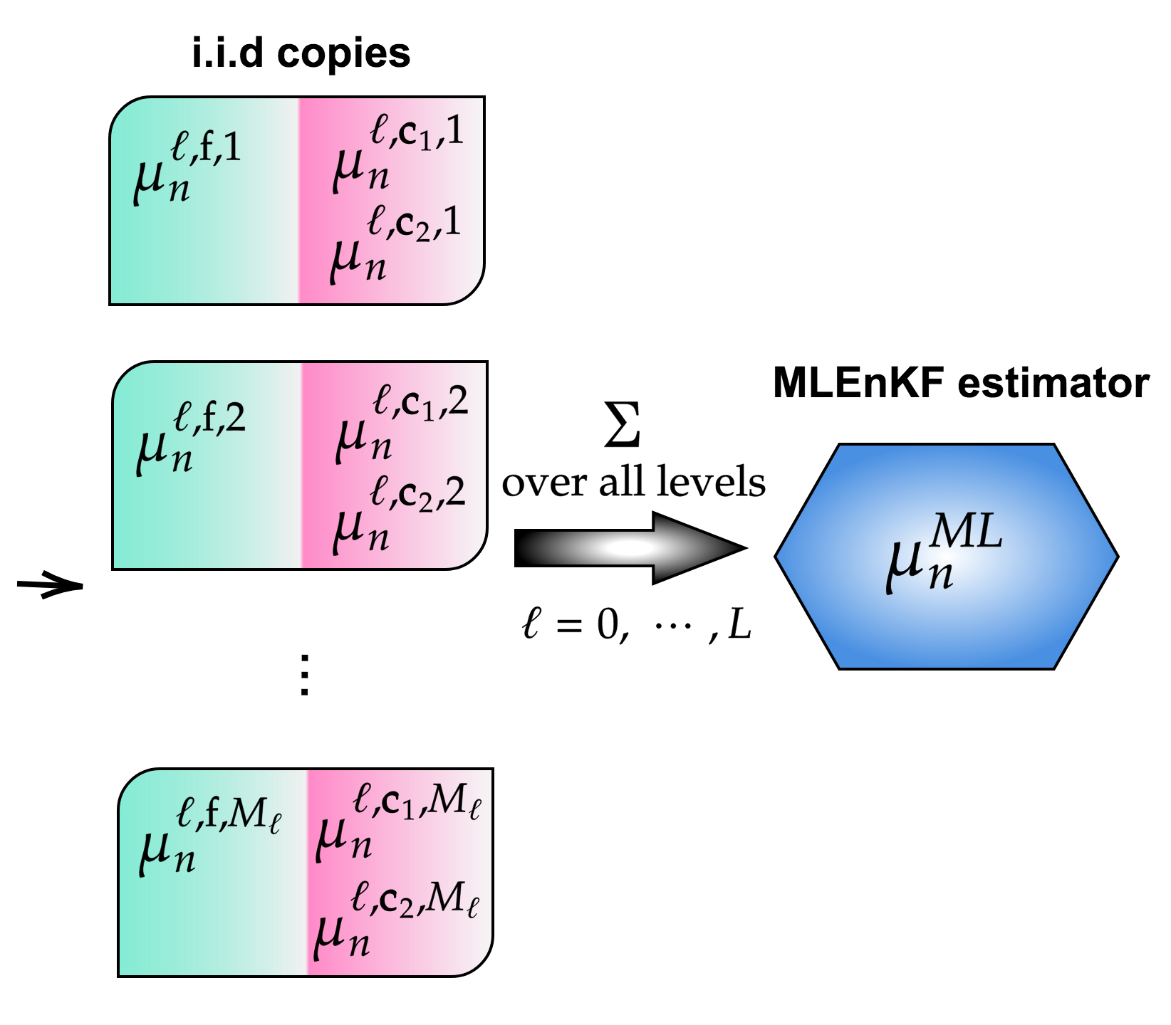
we obtain the MLEnKF estimator

(8) $$\begin{split}\mu^{ML}[\varphi]:=&\sum_{m=1}^{M_{0}}\frac{\mu_{n}^{N_{0},P_{0},m}[\varphi]}{M_{0}}\\ &+\sum_{\ell=1}^{L}\sum_{m=1}^{M_{\ell}}\frac{\mu_{n}^{N_{\ell},P_{\ell},m}[\varphi]}{M_{\ell}}-\frac{\Big{(}\mu_{n}^{N_{\ell-1},P_{\ell-1},1,m}+\mu_{n}^{N_{\ell-1},P_{\ell-1},2,m}\Big{)}[\varphi]}{2M_{\ell}}.\end{split}$$

As for classic MLMC estimators, the degrees of freedom $L$ and $\{M_{\ell}\}_{\ell=0}^{L}\subset\mathbb{N}$ are determined through a constrained optimization problem where one seeks to equilibrate the variance contribution from all of the sample averages and the bias error cf. Corollary 2. The purpose of pairwise-coupled particles is to reduce the variance of the MLEnKF estimator and thereby improve the efficiency of the method by reducing the number of samples $\{M_{\ell}\}$ needed to control the approximation error.

To describe the coupling between $\mu_{n}^{N_{\ell},P_{\ell}}$ and $(\mu_{n}^{N_{\ell-1},P_{\ell-1},1}$, $\mu_{n}^{N_{\ell-1},P_{\ell-1},2})$, we first introduce the following notation for the particles of the three underlying EnKF ensembles: for $\quad i=1,2\ldots,P_{\ell}$,

$$\begin{split}\hat{v}_{n,i}^{\ell,\mathbf{f}}&:=\hat{v}_{n,i}^{N_{\ell},P_{\ell}}\\ \hat{v}_{n,i}^{\ell,\mathbf{c}}&:=\begin{cases}\hat{v}_{n,i}^{\ell,\mathbf{c}_{1}}:=\hat{v}_{n,i}^{N_{\ell-1},P_{\ell-1},1}&\text{if}\quad i\leq P_{\ell-1}\\ \hat{v}_{n,i}^{\ell,\mathbf{c}_{2}}:=\hat{v}_{n,i-P_{\ell-1}}^{N_{\ell-1},P_{\ell-1},2}&\text{if}\quad P_{\ell-1}<i\leq P_{\ell},\end{cases}\end{split}$$

where $\hat{v}_{n,i}^{N_{\ell-1},P_{\ell-1},k}$ refers to the $i$-th updated particle at time $n$ of the EnKF measure $\mu_{n}^{N_{\ell-1},P_{\ell-1},k}$, for $k=1,2$. The superscript $\mathbf{f}$ refers to fine-level particles simulated with numerical resolution $N_{\ell}$ whereas $\mathbf{c}$ refers to the coarse-level particles simulated with numerical resolution $N_{\ell-1}$. The set of all the fine- and coarse-level particles are respectively denoted by

$$\hat{v}_{n,1:P_{\ell}}^{\ell,\mathbf{f}}:=\{\hat{v}_{n,i}^{\ell,\mathbf{f}}\}_{i=1}^{P_{\ell}}\quad\text{and}\quad\hat{v}_{n,1:P_{\ell}}^{\ell,\mathbf{c}}:=\{\hat{v}_{n,i}^{\ell,\mathbf{c}}\}_{i=1}^{P_{\ell}},$$

with the EnKF ensemble $\hat{v}_{n,1:P_{\ell}}^{\ell,\mathbf{f}}$ inducing the empirical measure $\mu_{n}^{\ell,\mathbf{f}}:=\mu_{n}^{N_{\ell},P_{\ell}}$. The set of all the coarse-level particles is a union of two EnKF ensembles with $P_{\ell-1}$ particles in each, namely $\hat{v}_{n,1:P_{\ell}}^{\ell,\mathbf{c}}=\hat{v}_{n,1:P_{\ell-1}}^{\ell,\mathbf{c}_{1}}\cup\hat{v}_{n,1:P_{\ell-1}}^{\ell,\mathbf{c}_{2}}$, where $\hat{v}_{n,1:P_{\ell-1}}^{\ell,\mathbf{c}_{1}}:=\{\hat{v}_{n,i}^{\ell,\mathbf{c}}\}_{i=1}^{P_{\ell-1}}$ and $\hat{v}_{n,1:P_{\ell-1}}^{\ell,\mathbf{c}_{2}}:=\{\hat{v}_{n,i}^{\ell,\mathbf{c}}\}_{i=P_{\ell-1}+1}^{P_{\ell}}$. The EnKF ensemble $\hat{v}_{n,1:P_{\ell}}^{\ell,\mathbf{c}_{k}}$ induces the empirical measure $\mu_{n}^{\ell,\mathbf{c}_{k}}:=\mu_{n}^{N_{\ell-1},P_{\ell-1},k}$ for $k=1,2$. By defining $\mu_{n}^{\ell,\mathbf{c}}:=\left(\mu_{n}^{\ell,\mathbf{c}_{1}}+\mu_{n}^{\ell,\mathbf{c}_{2}}\right)/2$ and imposing the convention

$$\mu_{n}^{0,\mathbf{c}}=\mu_{n}^{0,\mathbf{c}_{1}}=\mu_{n}^{0,\mathbf{c}_{2}}=0\quad\forall n\geq 0,$$

the MLEnKF estimator (8) can be written

(9) $$\begin{split}\mu_{n}^{\mathrm{ML}}[\varphi]=\sum_{\ell=0}^{L}\sum_{m=1}^{M_{\ell}}\frac{\mu_{n}^{\ell,\mathbf{f},m}[\varphi]-\mu_{n}^{\ell,\mathbf{c},m}[\varphi]}{M_{\ell}}\end{split}$$

where the sequence $\{(\mu_{n}^{\ell,\mathbf{f},m}[\varphi],\mu_{n}^{\ell,\mathbf{c},m}[\varphi])\}_{m}$ are iid draws from the joint distribution of coupled random variables $\mathbb{P}_{(\mu_{n}^{\ell,\mathbf{f}}[\varphi],\mu_{n}^{\ell,\mathbf{c}}[\varphi])}$.

2.4.1. One prediction-update iteration of pairwise coupled ensembles

For $\ell=0,1,\ldots,L$, the fine-level initial ensemble $\{\hat{v}_{0,i}^{\ell,\mathbf{f}}\}_{i=1}^{P_{\ell}}$ is independent and identically $\mathbb{P}_{u_{0}|Y_{0}}$-distributed and it is pairwise coupled to the coarse-level initial ensemble through setting $\hat{v}_{0,i}^{\ell,\mathbf{f}}=\hat{v}_{0,i}^{\ell,\mathbf{c}}$. For pairwise-coupled updated-state particles $\hat{v}_{n,i}^{\ell,\mathbf{f}}$ and $\hat{v}_{n,i}^{\ell,\mathbf{c}}$ at time $n$, we denote by the next-time prediction state respectively by $v^{\ell,\mathbf{f}}_{n+1,i}$ and $v^{\ell,\mathbf{c}}_{n+1,i}$. The prediction state is obtained by simulation of model dynamics on neighboring resolutions:

(10) $$\left.\begin{split}v^{\ell,\mathbf{f}}_{n+1,i}&=\Psi^{N_{\ell}}_{n}(\hat{v}^{\ell,\mathbf{f}}_{n,i})\\ v^{\ell,\mathbf{c}}_{n+1,i}&=\Psi^{N_{\ell-1}}_{n}(\hat{v}^{\ell,\mathbf{c}}_{n,i})\end{split}\right\}\quad i=1,\ldots,P_{\ell}.$$

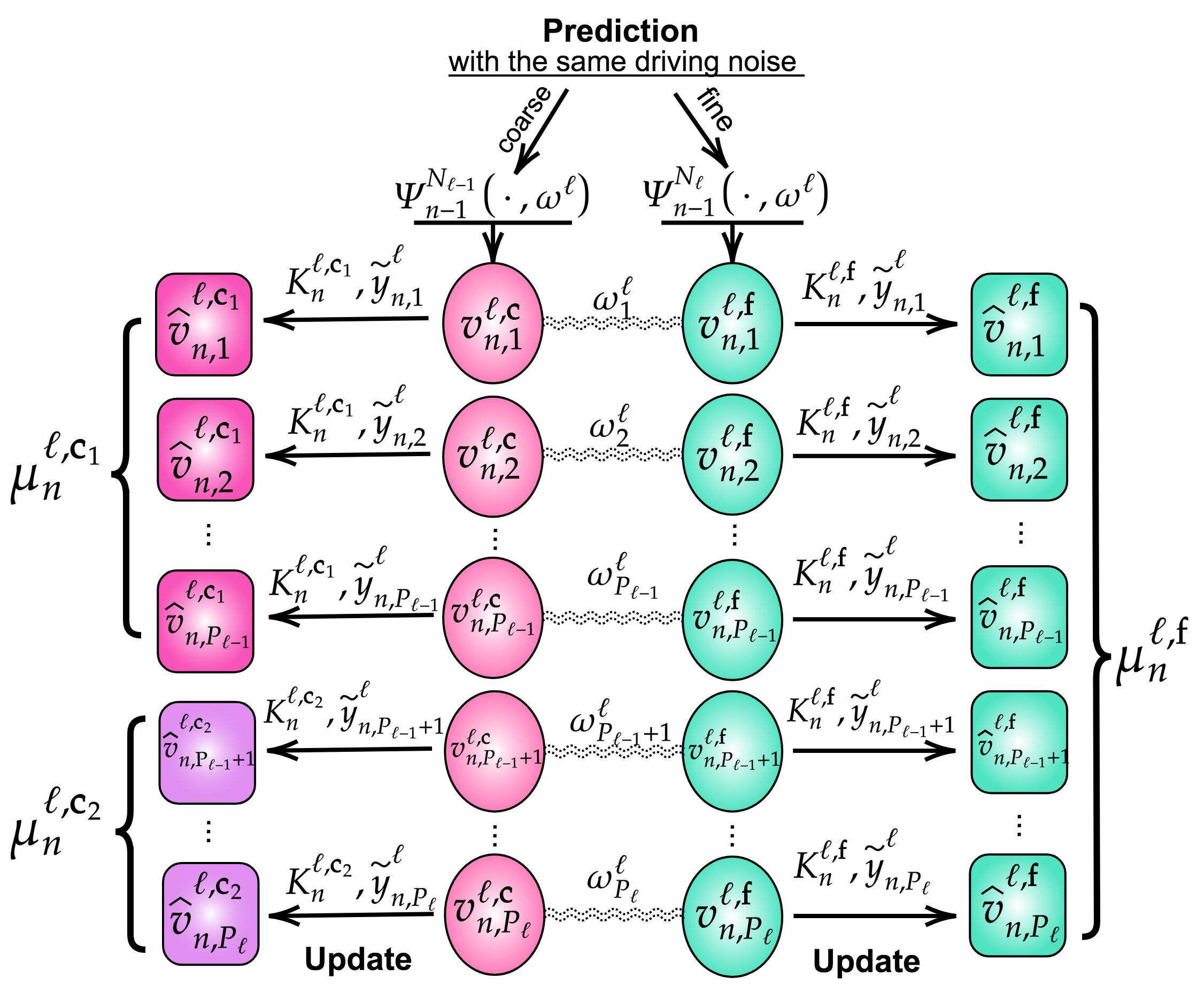
The simulations are pairwise coupled through sharing the same driving noise $W$. Then the sample covariance matrices and Kalman gains for the respective ensembles are computed by

$$\begin{split}C_{n+1}^{\ell,\mathbf{f}}=\overline{\mathrm{Cov}}[v^{\ell,\mathbf{f}}_{n+1}],\qquad K_{n+1}^{\ell,\mathbf{f}}&=C_{n+1}^{\ell,\mathbf{f}}H^{\mathbf{T}}(HC_{n+1}^{\ell,\mathbf{f}}H^{\mathbf{T}}+\Gamma)^{-1},\\ C_{n+1}^{\ell,\mathbf{c_{1}}}=\overline{\mathrm{Cov}}[v^{\ell,\mathbf{c_{1}}}_{n+1}],\qquad K_{n+1}^{\ell,\mathbf{c_{1}}}&=C_{n+1}^{\ell,\mathbf{c_{1}}}H^{\mathbf{T}}(HC_{n+1}^{\ell,\mathbf{c_{1}}}H^{\mathbf{T}}+\Gamma)^{-1},\\ C_{n+1}^{\ell,\mathbf{c_{2}}}=\overline{\mathrm{Cov}}[v^{\ell,\mathbf{c_{2}}}_{n+1}],\qquad K_{n+1}^{\ell,\mathbf{c_{2}}}&=C_{n+1}^{\ell,\mathbf{c_{2}}}H^{\mathbf{T}}(HC_{n+1}^{\ell,\mathbf{c_{2}}}H^{\mathbf{T}}+\Gamma)^{-1},\end{split}$$

where the sample covariances are defined in a similar fashion as in for EnKF:

(11) $$\begin{split}\overline{\mathrm{Cov}}[v^{\ell,\mathbf{f}}_{n+1}]:&=\sum_{i=1}^{P_{\ell}}\frac{v^{\ell,\mathbf{f}}_{n+1,i}\left(v^{\ell,\mathbf{f}}_{n+1,i}\right)^{\mathbf{T}}}{P_{\ell}}-\sum_{i=1}^{P_{\ell}}\frac{v^{\ell,\mathbf{f}}_{n+1,i}}{P_{\ell}}\left(\sum_{i=1}^{P_{\ell}}\frac{v^{\ell,\mathbf{f}}_{n+1,i}}{P_{\ell}}\right)^{\mathbf{T}},\\ \overline{\mathrm{Cov}}[v^{\ell,\mathbf{c_{j}}}_{n+1}]:&=\sum_{i=1}^{P_{\ell-1}}\frac{v^{\ell,\mathbf{c_{j}}}_{n+1,i}\left(v^{\ell,\mathbf{c_{j}}}_{n+1,i}\right)^{\mathbf{T}}}{P_{\ell-1}}-\sum_{i=1}^{P_{\ell-1}}\frac{v^{\ell,\mathbf{c_{j}}}_{n+1,i}}{P_{\ell-1}}\left(\sum_{i=1}^{P_{\ell-1}}\frac{v^{\ell,\mathbf{c_{j}}}_{n+1,i}}{P_{\ell-1}}\right)^{\mathbf{T}},\quad j=1,2.\end{split}$$

And the new observation $y_{n+1}$ is assimilated into the filter in the update step:

(12) $$\begin{split}&\left.\begin{split}\tilde{y}_{n+1,i}^{\ell}&=y_{n+1}+\eta_{n+1,i}^{\ell}\\ \hat{v}_{n+1,i}^{\ell,\mathbf{f}}&=(I-K_{n+1}^{\ell,\mathbf{f}}H)v^{\ell,\mathbf{f}}_{n+1,i}+K_{n+1}^{\ell,\mathbf{f}}\tilde{y}_{n+1,i}^{\ell}\end{split}\right\}\quad i=1,...,P_{\ell},\\ &\left.\begin{split}\hat{v}_{n+1,i}^{\ell,\mathbf{c_{1}}}&=(I-K_{n+1}^{\ell,\mathbf{c_{1}}}H)v_{n+1,i}^{\ell,\mathbf{c_{1}}}+K_{n+1}^{\ell,\mathbf{c_{1}}}\tilde{y}_{n+1,i}^{\ell}\\ \hat{v}_{n+1,i}^{\ell,\mathbf{c_{2}}}&=(I-K_{n+1}^{\ell,\mathbf{c_{2}}}H)v_{n+1,i}^{\ell,\mathbf{c_{2}}}+K_{n+1}^{\ell,\mathbf{c_{2}}}\tilde{y}_{n+1,i+P_{\ell-1}}^{\ell}\end{split}\right\}\quad i=1,...,P_{\ell-1},\end{split}$$

where $\{\eta_{n,i}^{\ell}\}_{n,\ell,i}$ are iid $N(0,\Gamma)$-distributed random variables. We note that the pairwise coupling of fine- and coarse-level particles is obtained through them sharing the same initial condition, driving noise $W$ in the dynamics (10), and perturbed observations. And to further elaborate on the relation between pairwise-coupled particles and pairwise-coupled EnKF estimators, the numerator in the $(\ell,m)$-th summand/sample of (9) takes the following form when represented in terms of its particles:

$$\mu_{n}^{\ell,\mathbf{f},m}[\varphi]-\mu_{n}^{\ell,\mathbf{c},m}[\varphi]=\begin{cases}P_{0}^{-1}\sum_{i=1}^{P_{0}}\varphi(\hat{v}^{0,\mathbf{f},m}_{n,i})&\text{if}\quad\ell=0\\ P_{\ell}^{-1}\sum_{i=1}^{P_{\ell}}\varphi(\hat{v}^{\ell,\mathbf{f},m}_{n,i})-\varphi(\hat{v}^{\ell,\mathbf{c},m}_{n,i})&\text{if}\quad\ell\geq 1.\end{cases}$$

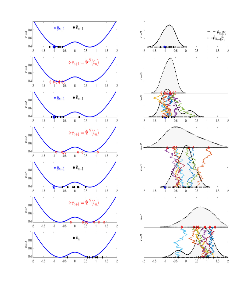
The motivation for pairwise-coupled particles is primarily to reduce the variance of the above sample/summand numerators $\varphi(\hat{v}_{n}^{\ell,\mathbf{f},m})-\varphi(\hat{v}_{n}^{\ell,\mathbf{c},m})$, and ultimately to improve the efficiency of your MLEnKF estimator. Provided the variance of these terms are substantially reduced, the number of samples $\{M_{\ell}\}$ needed to achieve a certain accuracy with your MLEnKF estimator may be lowered substantially, and this will improve the efficiency of your MLEnKF estimator. See Figure 2 for an illustration of one prediction-update iteration of the full MLEnKF estimator.

Figure 2. One prediction-update iteration of the MLEnKF estimator described in Section 2.4.1. Green and pink ovals represent fine- and coarse-level prediction-state particles, respectively, sharing the same initial condition and driving noise $\omega^{\ell}$ and the respective squares represent fine- and coarse-level updated-state particles sharing the perturbed observartions. The MLEnKF estimator is obtained by iid copies of pairwise-coupled samples, cf (9).

Remark 2.

For the herein-introduced MLEnKF method all the EnKF estimators $\{\mu^{\ell,\cdot,m}[\varphi]\}_{\ell,m}$ are independent for different $(\ell,m)-$samples. This in particular implies that also all Kalman gains and particles from different $(\ell,m)$-samples are independent. For the “canonical” MLEnKF method [22], on the other hand, all the particles in the full estimator are updated using the one shared Kalman gain. Therefore, the particles in the “canonical” MLEnKF method are all correlated, while all particles from different $(\ell,m)$-samples in the herein-introduced estimator are independent. The more extensive independence properties of the new MLEnKF estimator simplifies the proofs of asymptotic convergence results and in some settings also improves theoretical complexity bounds. See Corollary 2 and Remark 6 for a comparison of the theoretical complexity of the two methods.

2.5. Main results

We now present the main convergence and complexity results for EnKF and MLEnKF. The proofs for these results are provided in Appendix B. We will need the following assumptions:

Assumption 2.

For any exponentially-growing sequence $\{N_{\ell}\}$ of natural numbers, there exists a constant $c_{\Psi}>0$ and $\beta>0$ such that for all $\ell\in\mathbb{N}_{0}\cup\{\infty\}$, $n\in\mathbb{N}_{0}$, and $p\geq 2$,

• for all $|\kappa|_{1}\leq 1$,

  $$\left\|\partial^{\kappa}\Psi^{N_{\ell}}_{n}(u)\right\|_{p}\leq c_{\Psi}(1+\left\|u\right\|_{p})\quad\forall u\in L^{p}_{n}(\Omega,\mathbb{R}^{d}),$$

• for all $|\kappa|_{1}=2$,

  $$\left\|\partial^{\kappa}\Psi^{N_{\ell}}_{n}(u)\right\|_{p}\leq c_{\Psi}(1+\left\|u\right\|_{2p})\quad\forall u\in L^{2p}_{n}(\Omega,\mathbb{R}^{d}),$$

• for all $|\kappa|_{1}\leq 1$,

  $$\left\|\partial^{\kappa}\Psi^{N_{\ell+1}}_{n}(u)-\partial^{\kappa}\Psi^{N_{\ell}}_{n}(u)\right\|_{p}\leq c_{\Psi}(1+\left\|u\right\|_{p})N_{\ell}^{-\beta/2}\quad\forall u\in L^{p}_{n}(\Omega,\mathbb{R}^{d}).$$

Remark 3.

If the dynamics (1) is given by the SDE in Remark 1 and $\Psi^{N}_{n}$ denotes the corresponding Euler-Maruyama numerical solution, then Assumption 2 holds with $\beta=1$, cf. [45, 23, 24, 21].

Theorem 1 (Convergence of EnKF).

If Assumption 1 holds, then for any $\varphi\in\mathbb{F}$, $p\geq 2$ and $n\in\mathbb{N}_{0}$,

(13) $$\|\mu^{N,P}_{n}[\varphi]-\bar{\mu}_{n}[\varphi]\|_{p}\lesssim P^{-1/2}+N^{-\alpha},$$

where the hidden constant in $\lesssim$ depends on $p$, $n$ and $d$ (but not on $N$ and $P$).

Corollary 1.

If Assumption 1 holds, then $N\eqsim\epsilon^{-1/\alpha}$ and $P\eqsim\epsilon^{-2}$ ensure that

$$\|\mu^{N,P}_{n}[\varphi]-\bar{\mu}_{n}[\varphi]\|_{p}\lesssim\epsilon$$

for any $\varphi\in\mathbb{F}$, $p\geq 2$ and $n\in\mathbb{N}_{0}$. The resulting computational cost is

$$\mathrm{Cost}(\mathrm{EnKF})\eqsim\epsilon^{-(2+\frac{1}{\alpha})}.$$

Remark 4.

The proof of Theorem 1 shows that Theorem 1 and Corollary 1 apply even if the constraint $\mathbb{F}\subset C^{2}_{P}(\mathbb{R}^{d},\mathbb{R})$ in Assumption 1(ii) is weakened to $\mathbb{F}\subset C^{1}_{P}(\mathbb{R}^{d},\mathbb{R})$.

Theorem 2 (Convergence of MLEnKF).

If Assumptions 1 and 2 hold, then for any $L\geq 1$ and triplet of sequences $\{M_{\ell}\},\{N_{\ell}\},\{P_{\ell}\}\subset\mathbb{N}$ with $P_{\ell}\eqsim 2^{\ell}$ and exponentially-growing $N_{\ell}$, it holds for any $\varphi\in\mathbb{F}$, $n\geq 0$, and $p\geq 2$ that

$$\|\mu_{n}^{\mathrm{ML}}[\varphi]-\overline{\mu}_{n}[\varphi]\|_{p}\lesssim N_{L}^{-\beta/2}P_{L}^{-1/2}+P_{L}^{-1}+N_{L}^{-\alpha}+\sum_{\ell=0}^{L}M_{\ell}^{-1/2}(N_{\ell}^{-\beta/2}P_{\ell}^{-1/2}+P_{\ell}^{-1}),$$

where the hidden constant in $\lesssim$ depends on $p$, $n$ and $d$ (but not on $\{M_{\ell}\},\{N_{\ell}\},\{P_{\ell}\}$ and $L$).

Remark 5.

In Appendix B, the Theorems 1 and 2 are for simplicity proved for EnKF and MLEnKF methods using biased sample covariances, precisely as introduced in (7) and (11), respectively. However, the proofs can easily be extended, without any changes in convergence rates, to methods that instead use unbiased sample covariances, cf. Remark 7.

Corollary 2.

If Assumptions 1 and 2 hold, then for any $\epsilon,s>0$, the configuration $L=\left\lceil\frac{\log_{2}(\epsilon^{-1})}{\min(1,(1+\beta s)/2,\alpha s)}\right\rceil$, $P_{\ell}\eqsim 2^{\ell}$, $N_{\ell}\eqsim 2^{s\ell}$ and

(14) $$M_{\ell}\eqsim\begin{cases}\epsilon^{-2}\,2^{-{\frac{3+2s+\min(\beta s,1)}{3}\ell}}+1&\text{if }\min(\beta s,1)>s,\\ \epsilon^{-2}L^{2}2^{-(1+s)\ell}+1,&\text{if }\min(\beta s,1)=s,\\ \epsilon^{-2-{\frac{2(s-\min(\beta s,1))}{3\min(1,(1+\beta s)/2,\alpha s)}}}\,2^{-{\frac{3+2s+\min(\beta s,1)}{3}\ell}}+1,&\text{if }\min(\beta s,1)<s,\end{cases}$$

ensures that for any $\varphi\in\mathbb{F}$, $n\geq 0$ and $p\geq 2$,

(15) $$\|\mu^{\rm ML}_{n}[\varphi]-\bar{\mu}_{n}[\varphi]\|_{p}\lesssim\epsilon.$$

Moreover, if one sets the parameter $s$ such that

(16) $$s\in\begin{cases}[\alpha^{-1},1)&\text{if }\beta>1\quad\&\quad\alpha>1,\\ [\alpha^{-1},1]&\text{if }(\beta>1\quad\&\quad\alpha=1)\text{ or }(\beta=1\text{ and }\alpha\geq 1),\\ \{\alpha^{-1}\}&\text{if }(\beta\geq 1\quad\&\quad\alpha<1)\text{ or }(\beta<1\text{ and }\alpha\leq\beta),\\ \{(2\alpha-\beta)^{-1}\}&\text{if }\beta<1\quad\&\quad\alpha>\beta,\end{cases}$$

then the cost of the MLEnKF estimator is bounded by

(17) $$\mathrm{Cost}(\mathrm{MLEnKF})\eqsim\begin{cases}\epsilon^{-2}&\text{if }\beta>1\quad\&\quad\alpha>1,\\ \epsilon^{-2}|\log(\epsilon)|^{3}&\text{if }(\beta>1\quad\&\quad\alpha=1)\text{ or }(\beta=1\text{ and }\alpha\geq 1),\\ \epsilon^{-(1+1/\alpha)}&\text{if }(\beta\geq 1\quad\&\quad\alpha<1)\text{ or }(\beta<1\text{ and }\alpha\leq\beta),\\ \epsilon^{-(2+(1-\beta)/\alpha)}&\text{if }\beta<1\quad\&\quad\alpha>\beta.\end{cases}$$

The optimization of the parameter $s$ is stated in terms of inclusion sets in (16) as that may be useful for implementations. For further details on this optimization and the computational cost of the MLEnKF estimator, see Appendix B.3. The a priori cost-versus-accuracy results of Corollaries 1 and 2 show that in settings where both rates are sharp, MLEnKF will asymptotically have better complexity than EnKF.

Remark 6.

For comparison, we recall in compact form the cost-versus-accuracy result for the ”canonical” MLEnKF [22, Theorem 3.2]: For any $\epsilon>0$ and sufficiently smooth QoI $\varphi$ one may choose the estimator’s degrees of freedom so that

(18) $$\|\mu^{\rm ML^{OLD}}_{n}[\varphi]-\bar{\mu}_{n}[\varphi]\|_{p}\lesssim\epsilon,$$

where $\mu^{\rm ML^{OLD}}_{n}[\varphi]$ denotes the “canonical” MLEnKF estimator. The computational cost of achieving this accuracy is bounded by

(19) $$\mathrm{Cost}(\mathrm{MLEnKF^{OLD}})\eqsim\begin{cases}\left|\log(\epsilon)\right|^{2n}\epsilon^{-2},&\text{if}\quad\beta>1,\\ \left|\log(\epsilon)\right|^{2n+3}\epsilon^{-2},&\text{if}\quad\beta=1,\\ \Big{(}\epsilon/\left|\log(\epsilon)\right|^{2n}\Big{)}^{-\left(2+\frac{1-\beta}{\alpha}\right)},&\text{if}\quad\beta<1.\end{cases}$$

To achieve the same $\mathcal{O}(\epsilon)$-accuracy for the two MLEnKF methods, the theoretical bounds imply that for any $n\geq 2$ and any admissible $(\alpha,\beta)$-values with $\alpha\geq 1$,

$$\lim_{\epsilon\to 0}\frac{\mathrm{Cost}(\mathrm{MLEnKF^{NEW}})}{\mathrm{Cost}(\mathrm{MLEnKF^{OLD}})}=0.$$

In other words, if our theoretical bounds are sharp for both methods, then the new MLEnKF method asymptotically outperforms the “canonical” one in terms of computational cost versus accuracy. We note however that the regularity assumptions imposed for the new method’s hierarchy of numerical solvers, cf. Assumption 2, are more restrictive than those needed for the “canonical” method, and that we have previously made the conjecture that the error bounds for the “canonical” method are not sharp, cf. [22, Remark 3].

3. Numerical examples

In this section, we numerically compare the performance of MLEnKF and EnKF and (numerically) verify the results predicted by our theory. We will consider a couple of test problems with dynamics of the form

(20) $$u_{n+1}=\Psi(u_{n}):=u_{n}+\int_{n}^{n+1}-V^{\prime}(u_{t})dt+\int_{n}^{n+1}\sigma dW_{t},$$

where the potential $V\in C^{\infty}_{P}(\mathbb{R})$ satisfies $V^{\prime\prime}\in C^{\infty}_{B}(\mathbb{R})$, the diffusion coefficient is constant; $\sigma=0.5$, and linear observations (3) with $H=1$ and $\Gamma=0.1$. For any $N\geq 1$, $\Psi^{N}$ will in this section denote the Milstein numerical scheme with uniform timestep $\Delta t=1/N$. This yields the convergence rates $\alpha=1$, $\beta=2$.

For any $x\in\mathbb{R}$, let $\mathrm{Round}(x)$ denote the nearest integer to $x$. Given an input RMSE constraint $\epsilon>0$, we seek to equilibrate the magnitude of all error terms (cf. (13) for EnKF and Corollary 2 for MLEnKF) by setting the degrees of freedom to

(21) $$P=\mathrm{Round}(8\epsilon^{-2})\quad\text{and}\quad N=\mathrm{Round}(\epsilon^{-1})$$

for EnKF, and for MLEnKF we set $L=\mathrm{Round}(\log_{2}(\epsilon^{-1}))-1$, $N_{\ell}=2^{\ell+1}$, $P_{\ell}=10\times 2^{\ell}$, and

$$M_{\ell}=\begin{cases}2\mathrm{Round}(\epsilon^{-2}L^{2}2^{-3})&\text{if}\quad\ell=0\\ \mathrm{Round}(\epsilon^{-2}L^{2}2^{-2\ell-3})&\text{if}\quad 1\leq\ell\leq L.\end{cases}$$

Over a sequence of iterations $n=1,\ldots,\mathcal{N}$, we compare the performance of the methods in terms of error versus computer runtime (wall-clock time), where the error is measured in time-averaged-root-mean-squared error (RMSE):

$$\mbox{RMSE(EnKF)}:=\sqrt{\frac{1}{100(\mathcal{N}+1)}\sum_{i=1}^{100}\sum_{n=0}^{\mathcal{N}}\left|\mu^{N,P}_{n,i}[\varphi]-\bar{\mu}_{n}[\varphi]\right|^{2}}\lessapprox\mathrm{Runtime}^{-1/3},$$

where for a given $\epsilon>0$ with $\alpha=1$ and $\beta=2$, the last approximate asymptotic inequality follows from Corollary 1

$$\mbox{RMSE(EnKF)}\approx\left(\sum_{n=0}^{\mathcal{N}}\frac{\left\|\mu^{N,P}_{n}[\varphi]-\bar{\mu}_{n}[\varphi]\right\|_{2}^{2}}{\mathcal{N}+1}\right)^{1/2}\lesssim\epsilon\eqsim\mathrm{Cost}(\mathrm{EnKF})^{-1/3}.$$

Similarly,

$$\begin{split}\mbox{RMSE(MLEnKF)}&:=\sqrt{\frac{1}{100(\mathcal{N}+1)}\sum_{i=1}^{100}\sum_{n=0}^{\mathcal{N}}\left|\mu_{n,i}^{\rm ML}[\varphi]-\bar{\mu}_{n}[\varphi]\right|^{2}}\\ &\approx\left(\sum_{n=0}^{\mathcal{N}}\frac{\left\|\mu_{n}^{\rm ML}[\varphi]-\bar{\mu}_{n}[\varphi]\right\|_{2}^{2}}{\mathcal{N}+1}\right)^{1/2}\lesssim\log(10+\mathrm{Runtime})^{3/2}\mathrm{Runtime}^{-1/2},\end{split}$$

where the last inequality follows from Corollary 2, since it implies that

$$\mbox{RMSE(MLEnKF)}\lessapprox\epsilon\eqsim\log(\mathrm{Cost}(\mathrm{MLEnKF}))^{3/2}\mathrm{Cost}(\mathrm{MLEnKF})^{-1/2}.$$

Note here that $\{\mu_{.,i}^{N,P}[\varphi]\}_{i=1}^{100}$ and $\{\mu_{.,i}^{\rm ML}[\varphi]\}_{i=1}^{100}$ are computed using iid sequences of EnKF and MLEnKF empirical measures, respectively.

Reference solutions and computer architecture

For the first test problem we will consider, the dynamics $\Psi$ is linear. Therefore, we compute the exact reference solution $\bar{\mu}_{n}[\varphi]$ straightforwardly using the Kalman filter. The second test problem we will consider has nonlinear dynamics, and we need to approximate the reference solution. A pseudo-reference solution is then obtained by the deterministic mean-field EnKF (DMFEnKF) algorithm described in [35], cf. Appendix C.

The numerical simulations were computed in parallel on five cores on a Mac Pro with Quad-Core Intel Xeon X-5550 8-core processor with 16 GB of RAM. The computer code is written in the Julia programming language [4], and it can be downloaded from https://github.com/GaukharSH/mlenkf.

3.1. Ornstein-Uhlenbeck process

We consider the SDE (20) with $V(u)=u^{2}/2$, and the initial condition is $u_{0}\sim N(0,\Gamma)$. This is an Ornstein-Uhlenbeck (OU) process with the exact solution

$$\Psi(u_{n})=u_{n}e^{-t}+\int_{0}^{t}\sigma e^{s-t}dW_{s}.$$

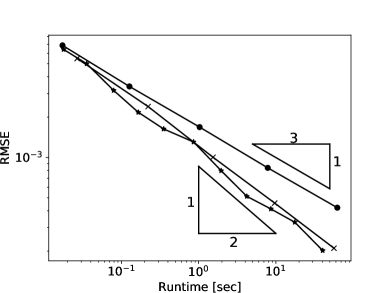
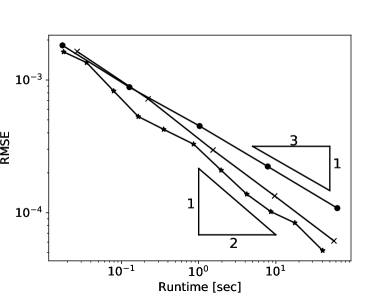
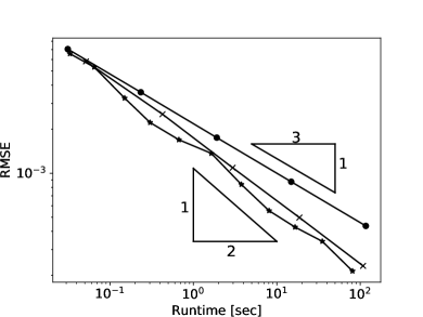
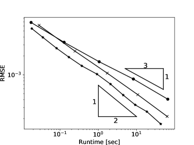
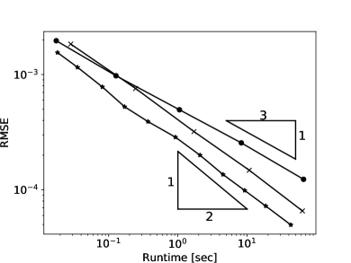
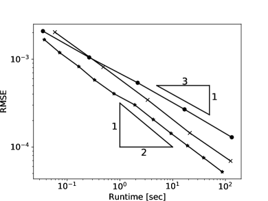
For a sequence of inputs, $\epsilon=[2^{-4},2^{-5},2^{-6},2^{-7},2^{-8}]$ for EnKF and MLEnKF, $\epsilon=[2^{-4},2^{-4.5},2^{-5},\ldots,2^{-9}]$ for ”canonical” MLEnKF, we study the performance of the three methods in terms of runtime versus RMSE over timeframes $\mathcal{N}=10$ and $\mathcal{N}=20$ observation times in Figure 3. For both QoI considered (the mean and the variance), the observations are in agreement with Corollaries 1 and 2, and Remark 6. The new MLEnKF method performs similarly as the “canonical” MLEnKF method and that both methods asymptotically outperform EnKF.

Figure 3. Top row: comparison of the runtime versus RMSE for the QoIs mean (left) and variance (right) over $\mathcal{N}=10$ observation times for the problem in Section 3.1. The solid-crossed line represents MLEnKF, the solid-asterisk line represents ”canonical” MLEnKF and the bottom reference triangle with the slope $\frac{1}{2}$, the solid-bulleted line represents EnKF and the upper reference triangle with the slope $\frac{1}{3}$. Bottom row: similar plots over $\mathcal{N}=20$ observation times.

3.2. Double-well SDE

We consider the SDE  (20) with the double-well potential

$$V(u)=\frac{1}{2+4u^{2}}+\frac{u^{2}}{4}$$

and $u_{0}\sim N(0,\Gamma)$. This SDE is the metastable motion of particles between the two wells, cf. [8, 44]. Figure 4 shows the dynamics of a particle over $\mathcal{N}=20$ observation times. We observe that the particle remains in either one of the wells for a relatively long time; in other words, transitions between wells happen quite rarely.

Figure 4. Realization of the double-well SDE from Section 3.2 over time $\mathcal{N}=20$ observation times (solid line) and observations (dots).

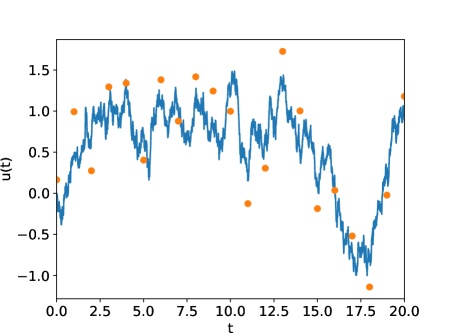
Figure 5 illustrates the well transition of an EnKF ensemble over a few predict-update iterations when the observations and the majority of the ensemble’s particles are located in opposite wells for the first few iterations.

Figure 5. Left column: Well transition of the EnKF ensemble when the measurements are located in the opposite well. Right column: Animation of the particle paths of the EnKF ensemble during the well-transition, and the resulting kernel density estimations of the EnKF prediction and update densities (Section 3.2).

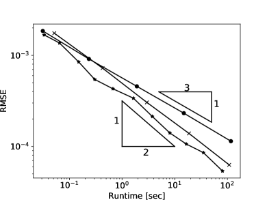
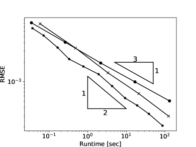
Using the same $\epsilon$-input sequences as in the preceding example, we study the performance of the three methods in terms of runtime versus RMSE over timeframes of $\mathcal{N}=10$ and $\mathcal{N}=20$ observation times in Figure 6. Once again, the work rates are in agreement with theory (Corollaries 1, 2 and Remark 6), that the new MLEnKF method performs similarly as the “canonical” MLEnKF method, and that both methods asymptotically outperform EnKF.

Figure 6. Top row: comparison of the runtime versus RMSE for the QoIs mean (left) and variance (right) over $\mathcal{N}=10$ observation times for the problem in Section 3.2. The solid-crossed line represents MLEnKF, the solid-asterisk line represents ”canonical” MLEnKF and the bottom reference triangle with the slope $\frac{1}{2}$, the solid-bulleted line represents EnKF and the upper reference triangle with the slope $\frac{1}{3}$. Bottom row: similar plots over $\mathcal{N}=20$ observation times

Appendix A Mean-field EnKF

The large-ensemble-limit of EnKF is referred to as the mean-field EnKF (MFEnKF). In the mean-field limit, the EnKF Kalman gain becomes a deterministic matrix. Consequently, there is no mixing between ensemble particles and the particles become iid. To describe the dynamics of MFEnKF, it thus suffices to consider a single particle. For fixed dynamics resolution $\Psi^{N}$, let $\hat{\bar{v}}_{n}^{N}$ denote the updated state of a mean-field particle at time $n$. The MFEnKF prediction and update dynamics is given by

(22) $$\bar{v}_{n+1}^{N}=\Psi^{N}_{n}(\hat{\bar{v}}_{n}^{N}),$$

and

$$\hat{\bar{v}}^{N}_{n+1}=(I-\bar{K}_{n+1}^{N}H)\bar{v}^{N}_{n+1}+\bar{K}_{n+1}^{N}{\tilde{y}}_{n+1},$$

where

$$\bar{K}_{n+1}^{N}={\bar{C}^{N}}_{n+1}H^{\mathbf{T}}\left(H{{\bar{C}^{N}}}_{n+1}H^{\mathbf{T}}+\Gamma\right)^{-1}\\$$

denotes the deterministic mean-field Kalman gain,

$$\bar{C}_{n+1}^{N}=\mathbb{E}\left[\left(\bar{v}^{N}_{n+1}-\mathbb{E}\left[{\bar{v}}^{N}_{n+1}\right]\right)\left({\bar{v}}^{N}_{n+1}-\mathbb{E}\left[{\bar{v}}^{N}_{n+1}\right]\right)^{\mathbf{T}}\right]$$

is the mean-field prediction covariance, and

$$\tilde{y}_{n+1}=y_{n+1}+\tilde{\eta}_{n+1}$$

denotes the perturbed observation with $\{\tilde{\eta}_{n}\}_{n=1}^{N}$ being independent and $N(0,\Gamma)-$distributed random variables satisfying $\tilde{\eta}_{j}\perp u_{k}$ for all $j,k\geq 0$.

By Assumption 1 (i) with $|\kappa|_{1}=0$, and using that $L_{n}^{p}(\Omega,\mathbb{R}^{d})\subset L^{p}(\Omega,\mathbb{R}^{d})$, it follows straightforwardly by induction that $\bar{v}_{n}^{N},\hat{\bar{v}}_{n}^{N}\in\cap_{p\geq 2}L^{p}(\Omega,\mathbb{R}^{d})$ uniformly in $N\in\mathbb{N}\cup\{\infty\}$:

(23) $$\begin{split}\hat{\bar{v}}_{0}^{N}\sim\mathbb{P}_{u_{0}|Y_{0}}&\implies\bar{v}_{1}^{N}=\Psi^{N}_{0}(\hat{\bar{v}}_{0}^{N})\in\cap_{p\geq 2}L^{p}(\Omega,\mathbb{R}^{d})\\ &\implies|\bar{C}_{1}^{N}|_{2}<\infty\implies|\bar{K}_{1}|_{2}<\infty\\ &\implies\|\hat{\bar{v}}^{N}_{1}\|_{p}\leq c_{p}(1+|H|_{2})\left(\|\bar{v}^{N}_{1}\|_{p}+\|\tilde{y}_{1}\|_{p}\right)<\infty\quad\forall p\geq 2\\ &\implies\ldots\implies\hat{\bar{v}}_{n}^{N}\in\cap_{p\geq 2}L^{p}(\Omega,\mathbb{R}^{d}).\end{split}$$

This ensures the existence of the mean-field measure $\bar{\mu}_{n}^{N}$, i.e., the distribution $\hat{\bar{v}}_{n}^{N}\sim\bar{\mu}_{n}^{N}$ satisfies $\hat{\bar{v}}_{n}^{N}\in\cap_{p\geq 2}L^{p}(\Omega,\mathbb{R}^{d})$ for all $N\in\mathbb{N}\cup\{\infty\}$ and $n\in\mathbb{N}_{0}$. For evaluating the expectation of a QoI $\varphi:\mathbb{R}^{d}\to\mathbb{R}$ wrt to the mean-field measure $\bar{\mu}_{n}^{N}$, we recall from Notation 2 that

$$\bar{\mu}_{n}^{N}[\varphi]=\int_{\mathbb{R}^{d}}\varphi(v)\bar{\mu}_{n}^{N}(dv).$$

For a subset of nonlinear dynamics $\Psi$ with additive Gaussian noise, it has been shown that in the large-ensemble limit, EnKF with perturbed observations converges to the Kalman filtering distribution with the standard rate $\mathcal{O}(P^{-1/2})$, cf. [36]. That is, in $L^{p}$ for all QoI $\varphi:\mathbb{R}^{d}\to\mathbb{R}$ with sufficient regularity $n\in\mathbb{N}_{0}$, and $p\geq 2$

$$\left\|\mu_{n}^{\infty,P}[\varphi]-\bar{\mu}_{n}[\varphi]\right\|_{p}\leq c_{\varphi,p}P^{-1/2}\quad\text{for some}\quad C_{\varphi,\Psi^{\infty}}>0,$$

where $\bar{\mu}_{n}:=\bar{\mu}_{n}^{\infty}$. The result was extended to a subset of fully non-Gaussian models [35] with numerical approximations of the dynamics in [22], i.e., $\mu^{N,P}_{n}[\varphi]\to\bar{\mu}_{n}[\varphi]$ as $P,N\to\infty$ (see also Theorem 1).

Appendix B Theoretical proofs

B.1. EnKF

In this section, we present a collection of theoretical results for EnKF that culminates with proof of Theorem 1.

Notation

The sample average of a QoI $\varphi\in\mathbb{F}$ applied to an ensemble of $P$ identically distributed particles $\{\hat{v}_{n,i}^{N,P}\}_{i=1}^{P}$ is defined as

$$E_{P}[\varphi(\hat{v}_{n}^{N,P})]:=\frac{1}{P}\sum_{i=1}^{P}\varphi(\hat{v}_{n,i}^{N,P})\quad(=\mu_{n}^{N,P}[\varphi]),$$

and similarly

(24) $$\begin{split}E_{P}[\hat{v}_{n}^{N,P}]:=\frac{1}{P}\sum_{i=1}^{P}\hat{v}_{n,i}^{N,P}\quad\mbox{ and }\quad E_{P}[\left(\hat{v}_{n}^{N,P}\right)\left(\hat{v}_{n}^{N,P}\right)^{\mathbf{T}}]:=\frac{1}{P}\sum_{i=1}^{P}\left(\hat{v}_{n,i}^{N,P}\right)\left(\hat{v}_{n,i}^{N,P}\right)^{\mathbf{T}}.\end{split}$$

Lemma 1 (Difference between EnKF and MFEnKF Kalman gains).

If Assumption 1 holds, then

$$\begin{split}\left\|K_{n}^{N,P}-\bar{K}_{n}^{N}\right\|_{p}&\leq|\Gamma^{-1}|_{2}|H|_{2}\left(1+2|\bar{K}_{n}^{N}H|_{2}\right)\left\|C_{n}^{N,P}-\bar{C}_{n}^{N}\right\|_{p}\lesssim\left\|C_{n}^{N,P}-\bar{C}_{n}^{N}\right\|_{p}\end{split}$$

for any $n\in\mathbb{N}_{0}$ and $p\geq 2$.

Proof.

The proof of the first inequality is analogous to [22, Lemma 3.4], and the latter inequality follows from $\bar{v}^{N}_{n}\in\cap_{p\geq 2}L^{p}(\Omega,\mathbb{R}^{d})$, uniformly in $N\geq 1$, cf. (23). ∎

We next bound the difference between $C_{n}^{N,P}=\overline{\mathrm{Cov}}[v_{n}^{N,P}]$ and $\bar{C}_{n}^{N}=\mathrm{Cov}[\bar{v}_{n}^{N}]$.

Lemma 2 (Difference between EnKF and MFEnKF covariance matrices).

If Assumption 1 holds, then

$$\left\|C_{n}^{N,P}-\bar{C}_{n}^{N}\right\|_{p}\lesssim\left\|v_{n}^{N,P}-\bar{v}_{n}^{N}\right\|_{2p}+P^{-\frac{1}{2}}$$

for any $n\in\mathbb{N}_{0}$ and $p\geq 2$.

Proof.

In order to bound $\left\|C_{n}^{N,P}-\bar{C}_{n}^{N}\right\|_{p}$, we introduce the auxiliary mean-field ensemble $\hat{\bar{v}}_{n,1:P}^{N,P}=\{\hat{\bar{v}}_{n,i}^{N,P}\}_{i=1}^{P}$ consisting of $P$ identically distributed particles whose prediction/update dynamics is given by the mean-field Kalman gain, namely

(25) $$\begin{split}\bar{v}^{N,P}_{n+1,i}&=\Psi^{N}_{n}(\hat{\bar{v}}_{n,i}^{N,P}),\\ \hat{\bar{v}}^{N,P}_{n+1,i}&=(I-\bar{K}^{N}_{n+1}H)\bar{v}^{N,P}_{n+1,i}+\bar{K}^{N}_{n+1}\tilde{y}_{n+1,i},\end{split}$$

with the initial condition $\hat{\bar{v}}^{N,P}_{0,i}=\hat{v}_{0,i}^{N,P}$ for $i=1,...,P$. The auxiliary ensemble satisfies the following two crucial properties: $\bar{v}_{n}^{N,P}\stackrel{{\scriptstyle D}}{{=}}\bar{v}_{n}$ and $\bar{v}_{n,i}^{N,P}$ has the same initial data, driving noise $W$ and perturbed observations as the $i$-th EnKF particle $v_{n,i}^{N,P}$, cf. Section 2.3. In other words, $\bar{v}_{n,i}^{N,P}$ is shadowing $v_{n,i}^{N,P}$.

Introducing the auxiliary ensemble covariance based on the mean-field prediction particles,

(26) $$\tilde{\bar{C}}_{n}^{N,P}:=\overline{\mathrm{Cov}}[\bar{v}_{n}^{N,P}],$$

the triangle inequality implies that

(27) $$\left\|C_{n}^{N,P}-\bar{C}_{n}^{N}\right\|_{p}\leq\left\|C_{n}^{N,P}-\tilde{\bar{C}}_{n}^{N,P}\right\|_{p}+\left\|\tilde{\bar{C}}_{n}^{N,P}-\bar{C}_{n}^{N}\right\|_{p}.$$

For the first term, recalling the notation (24), we have

$$\begin{split}\left\|C_{n}^{N,P}-\tilde{\bar{C}}_{n}^{N,P}\right\|_{p}&\leq\left\|E_{P}[v_{n}^{N,P}\big{(}(v_{n}^{N,P})^{\mathbf{T}}-(\bar{v}_{n}^{N,P})^{\mathbf{T}}\big{)}]\right\|_{p}+\left\|E_{P}[\big{(}v_{n}^{N,P}-\bar{v}_{n}^{N,P}\big{)}(\bar{v}_{n}^{N,P})^{\mathbf{T}}]\right\|_{p}\\ &+\left\|E_{P}[\bar{v}_{n}^{N,P}]E_{P}[(\bar{v}_{n}^{N,P})]^{\mathbf{T}}-E_{P}[\bar{v}_{n}^{N,P}]E_{P}[(v_{n}^{N,P})]^{\mathbf{T}}\right\|_{p}\\ &+\left\|E_{P}[\bar{v}_{n}^{N,P}]E_{P}[(v_{n}^{N,P})]^{\mathbf{T}}-E_{P}[v_{n}^{N,P}]E_{P}[(v_{n}^{N,P})]^{\mathbf{T}}\right\|_{p}.\end{split}$$

Jensen’s and Hölder’s inequalities and $\bar{v}_{n}^{N,P}\in L^{p}(\Omega,\mathbb{R}^{d})$ yield that

$$\begin{split}\left\|C_{n}^{N,P}-\tilde{\bar{C}}_{n}^{N,P}\right\|_{p}&\leq 2\left\|v_{n}^{N,P}\right\|_{2p}\left\|v_{n}^{N,P}-\bar{v}_{n}^{N,P}\right\|_{2p}+2\left\|\bar{v}_{n}^{N,P}\right\|_{2p}\left\|v_{n}^{N,P}-\bar{v}_{n}^{N,P}\right\|_{2p}\\ &\leq 2\left\|v_{n}^{N,P}-\bar{v}_{n}^{N,P}\right\|_{2p}^{2}+4\left\|\bar{v}_{n}^{N,P}\right\|_{2p}\left\|v_{n}^{N,P}-\bar{v}_{n}^{N,P}\right\|_{2p}\\ &\lesssim\max\left(\left\|v_{n}^{N,P}-\bar{v}_{n}^{N,P}\right\|_{2p}^{2},\left\|v_{n}^{N,P}-\bar{v}_{n}^{N,P}\right\|_{2p}\right).\end{split}$$

For the second term in (27), we have

$$\begin{split}\left\|\tilde{\bar{C}}_{n}^{N,P}-\bar{C}_{n}^{N}\right\|_{p}&\leq\left\|E_{P}[\bar{v}_{n}^{N,P}(\bar{v}_{n}^{N,P})^{\mathbf{T}}]-\mathbb{E}\left[\bar{v}_{n}^{N}(\bar{v}_{n}^{N})^{\mathbf{T}}\right]\right\|_{p}\\ &+\left\|E_{P}[\bar{v}_{n}^{N,P}]E_{P}[(\bar{v}_{n}^{N,P})^{\mathbf{T}}]-\mathbb{E}\left[\bar{v}_{n}^{N}\right]\mathbb{E}\left[(\bar{v}_{n}^{N})^{\mathbf{T}}\right]\right\|_{p}\\ &\lesssim P^{-\frac{1}{2}}\left\|\bar{v}_{n}^{N,P}(\bar{v}_{n}^{N,P})^{\mathbf{T}}\right\|_{p}\\ &\lesssim P^{-\frac{1}{2}}\left\|\bar{v}_{n}^{N,P}\right\|_{2p}^{2},\end{split}$$

where the penultimate inequality is obtained by the Marcinkiewicz-Zygmund (M-Z) inequality [32, Theorem 5.2]. The property $\bar{v}_{n}^{N,P}\in L^{p}(\Omega,\mathbb{R}^{d})$, together with the above inequalities imply that

(28) $$\left\|C_{n}^{N,P}-\bar{C}_{n}^{N}\right\|_{p}\lesssim\max(\left\|v_{n}^{N,P}-\bar{v}_{n}^{N,P}\right\|_{2p},\left\|v_{n}^{N,P}-\bar{v}_{n}^{N,P}\right\|_{2p}^{2})+P^{-\frac{1}{2}}.$$

Finally, by the proof of Lemma 3, it follows that $\left\|v_{n}^{N,P}-\bar{v}_{n}^{N,P}\right\|_{2p}\lesssim 1$ and thus

$$\left\|C_{n}^{N,P}-\bar{C}_{n}^{N}\right\|_{p}\lesssim\left\|v_{n}^{N,P}-\bar{v}_{n}^{N,P}\right\|_{2p}+P^{-\frac{1}{2}}.$$

∎

Remark 7.

Lemma 2 straightforwardly extends to EnKF methods using an unbiased sample prediction covariance $\mathcal{C}_{n}^{N,P}$. By the following relationship between biased and unbiased sample covariances

$$\mathcal{C}_{n}^{N,P}:=\frac{P}{P-1}C_{n}^{N,P},$$

we obtain that

$$\begin{split}\left\|\mathcal{C}_{n}^{N,P}-\bar{C}_{n}^{N}\right\|_{p}&\leq\left\|\mathcal{C}_{n}^{N,P}-C_{n}^{N,P}\right\|_{p}+\left\|C_{n}^{N,P}-\bar{C}_{n}^{N}\right\|_{p}\\ &=\frac{P}{P-1}\left\|C_{n}^{N,P}-\bar{C}_{n}^{N}\right\|_{p}+\frac{1}{P-1}\left\|\bar{C}_{n}^{N,P}\right\|_{p}.\end{split}$$

The first term in the last equality is bounded by Lemma 2, and the bound for the second term follows from $\bar{v}_{n}^{N,P}\in L^{p}(\Omega,\mathbb{R}^{d})$. In the proof of Theorem 1, the error contribution from the sample covariance, be that a biased or an unbiased one, only enters through Lemma 2. This implies that the theorem holds and the convergence rate is not affected when replacing biased with unbiased sample covariances in the EnKF method.

Moreover, in the proof of Theorem 2 for MLEnKF, the error contribution from sample covariances only enter through Corollary 3 and Lemma 8. By a similar argument as above, the rates of the said corollary and lemma are not affected by replacing biased sample covariances by unbiased ones and Theorem 2 will also holds with the same convergence rate.

Lemma 3 (Distance between ensembles).

If Assumption 1 holds, then

$$\max\left(\left\|\hat{v}_{n}^{N,P}-\hat{\bar{v}}_{n}^{N}\right\|_{p},\left\|v_{n}^{N,P}-\bar{v}_{n}^{N}\right\|_{p}\right)\lesssim P^{-1/2}\quad\text{for any}\quad n\in\mathbb{N}_{0}\quad\text{and}\quad p\geq 2.$$

Proof.

Since $\hat{v}_{0}^{N,P}=\hat{\bar{v}}_{0}^{N}$, the first half of the statement holds for $n=0$. Assume that for some $n\geq 1$, $\|\hat{v}_{n-1}^{N,P}-\hat{\bar{v}}_{n-1}^{N}\|_{p}\lesssim P^{-1/2}$ holds for all $p\geq 2$. Assumption 1(iii) then implies that

(29) $$\left\|v_{n}^{N,P}-\bar{v}_{n}^{N}\right\|_{p}\lesssim\left\|\hat{v}_{n-1}^{N,P}-\hat{\bar{v}}_{n-1}^{N}\right\|_{p}\lesssim P^{-\frac{1}{2}}.$$

By Hölder’s inequality and Lemma 1,

(30) $$\begin{split}\left\|\hat{v}_{n}^{N,P}-\hat{\bar{v}}_{n}^{N}\right\|_{p}&\lesssim|I-\bar{K}_{n}^{N}H|_{2}\left\|v_{n}^{N,P}-\bar{v}_{n}^{N}\right\|_{p}\\ &+\left\|C_{n}^{N,P}-\bar{C}_{n}^{N}\right\|_{2p}\big{(}\left\|v_{n}^{N,P}-\bar{v}_{n}^{N}\right\|_{2p}+\left\|\tilde{y}_{n}-H\bar{v}_{n}^{N}\right\|_{2p}\big{)}.\end{split}$$

Since $\bar{v}_{n}^{N},\tilde{y}_{n}^{\ell}\in\cap_{r\geq 2}L^{r}(\Omega)$, inequalities (29) and (28) imply that

$$\begin{split}\left\|\hat{v}_{n}^{N,P}-\hat{\bar{v}}_{n}^{N}\right\|_{p}&\lesssim(|I-\bar{K}_{n}^{N}H|_{2}+\left\|\tilde{y}_{n}-H\bar{v}_{n}^{N}\right\|_{2p})P^{-1/2}+P^{-1}\lesssim P^{-1/2}.\end{split}$$

The argument holds for any $p\geq 2$, and the proof follows by induction. ∎

Before proving the main convergence result for EnKF, we introduce the notation $\bar{\mu}_{n}^{N,P}[\varphi]$ to denote the average of the QoI $\varphi$ over the empirical measure associated with the auxiliary mean-field ensemble $\{\hat{\bar{v}}_{n,i}^{N}\}_{i=1}^{P}$, cf. (25), and we recall that $\bar{\mu}_{n}^{N}[\varphi]$ denotes the evaluation of empirical measure on QoI $\varphi$ associated with the MFEnKF $\hat{\bar{v}}_{n}^{N}$, cf. Section A.

Proof of Theorem 1.

By the triangle inequality,

$$\left\|\mu_{n}^{N,P}[\varphi]-\bar{\mu}_{n}[\varphi]\right\|_{p}\leq\left\|\mu_{n}^{N,P}[\varphi]-\bar{\mu}_{n}^{N,P}[\varphi]\right\|_{p}+\left\|\bar{\mu}_{n}^{N,P}[\varphi]-\bar{\mu}_{n}^{N}[\varphi]\right\|_{p}+\left\|\bar{\mu}_{n}^{N}[\varphi]-\bar{\mu}_{n}[\varphi]\right\|_{p}.$$

By Assumption 1(ii), $\varphi\in\mathbb{F}\subset C^{2}_{P}(\mathbb{R}^{d},\mathbb{R})$, and Lemma 3 implies that

$$\left\|\mu_{n}^{N,P}[\varphi]-\bar{\mu}_{n}^{N,P}[\varphi]\right\|_{p}=\left\|\frac{1}{P}\sum_{i=1}^{P}\varphi(\hat{v}_{n,i}^{N,P})-\varphi(\hat{\bar{v}}_{n,i}^{N})\right\|_{p}\leq c_{\varphi}\left\|\widehat{v}_{n}^{N,P}-\hat{\bar{v}}_{n}^{N}\right\|_{2p}\lesssim P^{-1/2}.$$

For the second term, using the Marcinkiewicz–Zygmund (M-Z) inequality, that $\varphi(\hat{\bar{v}}_{n}^{N})\in\cap_{p\geq 2}L^{p}(\Omega,\mathbb{R})$ and that $\hat{\bar{v}}_{n,1}^{N,P},\ldots,\hat{\bar{v}}_{n,P}^{N,P}$ are iid with $\hat{\bar{v}}_{n,i}^{N,P}\stackrel{{\scriptstyle D}}{{=}}\hat{\bar{v}}_{n}^{N}$ imply that

$$\left\|\bar{\mu}_{n}^{N,P}[\varphi]-\bar{\mu}_{n}^{N}[\varphi]\right\|_{p}=\left\|\sum_{i=1}^{P}\frac{\varphi(\hat{\bar{v}}_{n,i}^{N})-\mathbb{E}\left[\varphi(\hat{\bar{v}}_{n}^{N})\right]}{P}\right\|_{p}\lesssim P^{-1/2}.$$

For the last term, we have that

$$\left\|\bar{\mu}_{n}^{N}[\varphi]-\bar{\mu}_{n}[\varphi]\right\|_{p}=\left|\mathbb{E}\left[\varphi(\hat{\bar{v}}_{n}^{N})-\varphi(\hat{\bar{v}}_{n})\right]\right|,$$

and it remains to prove by induction that the right-hand side is $\mathcal{O}(N^{-\alpha})$.

Since $\hat{\bar{v}}_{0}^{N}\stackrel{{\scriptstyle D}}{{=}}\hat{\bar{v}}_{0}$, it holds that $\left|\mathbb{E}\left[\varphi(\hat{\bar{v}}_{0}^{N})-\varphi(\hat{\bar{v}}_{0})\right]\right|=0$. Assume that for some $k\geq 1$, there exists an observable dependent constant $c_{\varphi}>0$ such that

$$\left|\mathbb{E}\left[\varphi(\hat{\bar{v}}_{k-1}^{N})-\varphi(\hat{\bar{v}}_{k-1})\right]\right|\leq c_{\varphi}N^{-\alpha}\quad\forall\varphi\in\mathbb{F}.$$

Then, Assumption 1(ii) implies there exists a $\tilde{c}_{\varphi}>0$ such that

(31) $$\left|\mathbb{E}\left[\varphi(\bar{v}_{k}^{N})-\varphi(\bar{v}_{k})\right]\right|\leq\tilde{c}_{\varphi}N^{-\alpha}\quad\forall\varphi\in\mathbb{F}.$$

In order to bound $\left|\mathbb{E}\left[\varphi(\hat{\bar{v}}_{k}^{N})-\varphi(\hat{\bar{v}}_{k})\right]\right|$, we first recall that

$$\begin{split}\hat{\bar{v}}_{k}^{N}&=(I-\bar{K}_{k}^{N}H)\bar{v}_{k}^{N}+\bar{K}^{N}_{k}y_{n}+\bar{K}^{N}_{k}\tilde{\eta}_{k}\\ \hat{\bar{v}}_{k}&=(I-\bar{K}_{k}H)\bar{v}_{k}+\bar{K}_{k}y_{n}+\bar{K}_{k}\tilde{\eta}_{k},\end{split}$$

with $\tilde{\eta}_{k}\sim N(0,\Gamma)$ and introduce the functions $\tilde{\varphi}^{N},\tilde{\varphi}\in\mathbb{F}$ defined by

$$\tilde{\varphi}^{N}(x)=\frac{1}{\sqrt{(2\pi)^{p}|\mathrm{det}(\Gamma)|}}\int_{\mathbb{R}^{p}}\varphi\Big{(}(I-\bar{K}^{N}_{k}H)x+\bar{K}^{N}_{k}y_{k}+\bar{K}^{N}_{k}z\Big{)}e^{-z^{\mathbf{T}}\Gamma^{-1}z/2}\,dz$$

and

$$\tilde{\varphi}(x)=\frac{1}{\sqrt{(2\pi)^{p}|\mathrm{det}(\Gamma)|}}\int_{\mathbb{R}^{p}}\varphi\Big{(}(I-\bar{K}_{k}H)x+\bar{K}_{k}y_{k}+\bar{K}_{k}z\Big{)}e^{-z^{\mathbf{T}}\Gamma^{-1}z/2}\,dz.$$

It then follows by the mean-value theorem that

$$\begin{split}\left|\mathbb{E}\left[\varphi(\hat{\bar{v}}_{k}^{N})-\varphi(\hat{\bar{v}}_{k})\right]\right|&\leq\left|\mathbb{E}\left[\tilde{\varphi}^{N}(\bar{v}_{k}^{N})-\tilde{\varphi}^{N}(\bar{v}_{k})\right]\right|+\left|\mathbb{E}\left[\tilde{\varphi}^{N}(\bar{v}_{k})-\tilde{\varphi}(\bar{v}_{k})\right]\right|\\ &\lesssim N^{-\alpha}+|\bar{K}_{k}-\bar{K}^{N}_{k}|_{2}.\end{split}$$

From [22, Lemma 3.4], we have that

$$\bar{K}_{k}-\bar{K}^{N}_{k}=\bar{K}_{k}H(\bar{C}_{k}^{N}-\bar{C}_{k})H^{\mathbf{T}}(H\bar{C}_{k}^{N}H^{\mathbf{T}}+\Gamma)^{-1}+(\bar{C}_{k}-\bar{C}_{k}^{N})H^{\mathbf{T}}(H\bar{C}_{k}^{N}H^{\mathbf{T}}+\Gamma)^{-1},$$

which, since $\Gamma$ is positive definite and thus $|(H\bar{C}_{k}^{N}H^{\mathbf{T}}+\Gamma)^{-1}|_{2}\lesssim|\Gamma^{-1}|_{2}<\infty$, implies that

$$\begin{split}|\bar{K}_{k}-\bar{K}^{N}_{k}|_{2}&\lesssim|\bar{C}_{k}^{N}-\bar{C}_{k}|_{2}\\ &\leq\left|\mathbb{E}\left[\bar{v}^{N}_{k}(\bar{v}_{k}^{N})^{\mathbf{T}}-\bar{v}_{k}(\bar{v}_{k})^{\mathbf{T}}\right]\right|_{2}+\left|\mathbb{E}\left[\bar{v}^{N}_{k}\right]\mathbb{E}\left[(\bar{v}_{k}^{N})^{\mathbf{T}}\right]-\mathbb{E}\left[\bar{v}_{k}\right]\mathbb{E}\left[(\bar{v}_{k})^{\mathbf{T}}\right]\right|_{2}\\ &\lesssim N^{-\alpha}.\end{split}$$

Since all monomials of degree $1$ and $2$ are contained in $\mathbb{F}$, the last inequality follows from (31) and the equivalence of the Euclidean and Frobenius norms in any dimension $d<\infty$. It holds by induction that for any $n\geq 0$,

$$|\mathbb{E}[\varphi(\hat{\bar{v}}_{n}^{N})-\varphi(\hat{\bar{v}}_{n})]|\lesssim N^{-\alpha}.$$

∎

B.2. MLEnKF

In this section, we present a collection of theoretical results for MLEnKF, including the proof of Theorem 2.

In order to obtain a connection between $\{\hat{v}_{n,i}^{\ell,\mathbf{f}}\}_{i=1}^{P_{\ell}}$ and $\{\hat{v}_{n,i}^{\ell,\mathbf{c}}\}_{i=1}^{P_{\ell}}=\{\hat{v}_{n,i}^{\ell,\mathbf{c}_{1}}\}_{i=1}^{P_{\ell-1}}\cup\{\hat{v}_{n,i}^{\ell,\mathbf{c}_{2}}\}_{i=1}^{P_{\ell-1}}$ in the superindex $\mathbf{c}_{j}\leftrightarrow\mathbf{f}_{j}$, we introduce

$$\hat{v}_{n,i}^{\ell,\mathbf{f}_{1}}:=\hat{v}_{n,i}^{\ell,\mathbf{f}}\quad\text{and}\quad\hat{v}_{n,i}^{\ell,\mathbf{f}_{2}}:=\hat{v}_{n,i+P_{\ell-1}}^{\ell,\mathbf{f}}\quad\text{for}\quad i=1,\ldots,P_{\ell-1},$$

and

$$\mu_{n}^{\ell,\mathbf{f}_{j}}[\varphi]:=E_{P_{\ell-1}}[\varphi(\hat{v}_{n}^{\ell,\mathbf{f}_{j}})]=\frac{1}{P_{\ell-1}}\sum_{i=1}^{P_{\ell-1}}\varphi(\hat{v}_{n,i}^{\ell,\mathbf{f}_{j}})\quad\text{for}\quad j=1,2.$$

The random variable $\hat{v}_{n}^{\ell,\mathbf{f}_{j}}$ has the same driving noise and perturbed observations as $\hat{v}_{n}^{\ell,\mathbf{c}_{j}}$ and we note that

$$\begin{split}\left(\mu_{n}^{\ell,\mathbf{f}}-\frac{\mu_{n}^{\ell,\mathbf{c}_{1}}+\mu_{n}^{\ell,\mathbf{c}_{2}}}{2}\right)[\varphi]&=E_{P_{\ell}}[\varphi(\hat{v}_{n}^{\ell,\mathbf{f}})-\varphi(\hat{v}_{n}^{\ell,\mathbf{c}})]\\ &=\frac{1}{2}\sum_{j=1}^{2}\left(\mu_{n}^{\ell,\mathbf{f}_{j}}-\mu_{n}^{\ell,\mathbf{c}_{j}}\right)[\varphi].\end{split}$$

We further introduce the auxiliary mean-field MLEnKF ensemble $\{\hat{\bar{v}}^{\ell,\mathbf{f}}_{n,1:P_{\ell}},\hat{\bar{v}}^{\ell,\mathbf{c}}_{n,1:P_{\ell}}\}_{\ell=0}^{L}$ where the dynamics for $\hat{\bar{v}}^{\ell,\mathbf{f}}_{n,i}$ and $\hat{\bar{v}}^{\ell,\mathbf{c}}_{n,i}$ are coupled through driving-noise-sharing dynamics

(32) $$\bar{v}^{\ell,\mathbf{f}}_{n+1,i}=\Psi^{N_{\ell}}_{n}(\hat{\bar{v}}^{\ell,\mathbf{f}}_{n,i}),\qquad\bar{v}^{\ell,\mathbf{c}}_{n+1,i}=\Psi^{N_{\ell}}_{n}(\hat{\bar{v}}^{\ell,\mathbf{c}}_{n,i})$$

and perturbed-observation-sharing updates

(33) $$\hat{\bar{v}}^{\ell,\mathbf{f}}_{n+1,i}=(I-\bar{K}^{\ell,\mathbf{f}}_{n}H)\bar{v}^{\ell,\mathbf{f}}_{n,i}+\bar{K}^{\ell,\mathbf{f}}_{n}\tilde{y}_{n,i}^{\ell},\qquad\hat{\bar{v}}^{\ell,\mathbf{c}}_{n+1,i}=(I-\bar{K}^{\ell,\mathbf{c}}_{n}H)\bar{v}^{\ell,\mathbf{c}}_{n,i}+\bar{K}^{\ell,\mathbf{c}}_{n}\tilde{y}_{n,i}^{\ell},$$

where $\bar{K}^{\ell,\mathbf{f}}_{n}:=\bar{K}^{N_{\ell}}_{n}$ and $\bar{K}^{\ell,\mathbf{c}}_{n}:=\bar{K}^{N_{\ell-1}}_{n}$, cf. Section A, and with initial conditions equal identical to MLEnKF:

$$\begin{split}\hat{\bar{v}}^{0,\mathbf{f}}_{0,i}&:=\hat{v}_{0,i}^{\ell,\mathbf{f}}\\ \hat{\bar{v}}^{\ell,\mathbf{f}}_{0,i}=\hat{\bar{v}}^{\ell,\mathbf{c}}_{0,i}&:=\hat{v}_{0,i}^{\ell,\mathbf{f}}=\hat{v}_{0,i}^{\ell,\mathbf{c}}\quad\ell\geq 1.\end{split}$$

The particles $(\hat{\bar{v}}^{\ell,\mathbf{f}}_{n,i},\hat{\bar{v}}^{\ell,\mathbf{c}}_{n,i})$ are thus coupled through sharing the same initial condition, driving noise $W$, and perturbed observations. The particle pair is also coupled to the MLEnKF pair $(\hat{v}_{n,i}^{\ell,\mathbf{f}},\hat{v}_{n,i}^{\ell,\mathbf{c}})$ in all the same ways. In other words, $(\hat{\bar{v}}^{\ell,\mathbf{f}}_{n,i},\hat{\bar{v}}^{\ell,\mathbf{c}}_{n,i})$ is shadowing $(\hat{v}_{n,i}^{\ell,\mathbf{f}},\hat{v}_{n,i}^{\ell,\mathbf{c}})$. The ensemble $\hat{\bar{v}}^{\ell,\mathbf{f}}_{n,1:P_{\ell}}=\hat{\bar{v}}^{\ell,\mathbf{f}_{1}}_{n,1:P_{\ell-1}}\cup\hat{\bar{v}}^{\ell,\mathbf{f}_{2}}_{n,1:P_{\ell-1}}$ induces an empirical measure $\bar{\mu}_{n}^{\ell,\mathbf{f}}=(\bar{\mu}_{n}^{\ell,\mathbf{f}_{1}}+\bar{\mu}_{n}^{\ell,\mathbf{f}_{2}})/2$ and $\hat{\bar{v}}^{\ell,\mathbf{c}}_{n,1:P_{\ell}}=\hat{\bar{v}}^{\ell,\mathbf{c}_{1}}_{n,1:P_{\ell-1}}\cup\hat{\bar{v}}^{\ell,\mathbf{c}_{2}}_{n,1:P_{\ell-1}}$ induces $\bar{\mu}_{n}^{\ell,\mathbf{c}}=(\bar{\mu}_{n}^{\ell,\mathbf{c}_{1}}+\bar{\mu}_{n}^{\ell,\mathbf{c}_{2}})/2$, with the convention that $\bar{\mu}_{n}^{0,\mathbf{c}}=\bar{\mu}_{n}^{0,\mathbf{c}_{1}}=\bar{\mu}_{n}^{0,\mathbf{c}_{2}}=0$ for all $n\geq 0$. Employing sequences $\{M_{\ell}\},\{N_{\ell}\}\subset\mathbb{N}$ and $L\in\mathbb{N}$ with exactly the same values as those used for the MLEnKF estimator (9) we seek to shadow, we define the auxiliary mean-field MLEnKF estimator by

(34) $$\bar{\mu}^{\mathrm{ML}}_{n}[\varphi]=\sum_{\ell=0}^{L}\frac{1}{M_{\ell}}\sum_{m=1}^{M_{\ell}}\left(\bar{\mu}_{n}^{\ell,\mathbf{f},m}-\bar{\mu}_{n}^{\ell,\mathbf{c},m}\right)[\varphi]$$

where for $m=1,\ldots,M_{\ell}$, $\left(\bar{\mu}_{n}^{\ell,\mathbf{f},m}-\bar{\mu}_{n}^{\ell,\mathbf{c},m}\right)[\varphi]$ are iid realizations that are coupled to/shadowing $\left(\mu_{n}^{\ell,\mathbf{f},m}-\mu_{n}^{\ell,\mathbf{c},m}\right)[\varphi]$ by sharing the same underlying randomness (initial conditions, driving noise and perturbed observations). And, consequently, $\bar{\mu}^{\mathrm{ML}}_{n}[\varphi]$ is shadowing $\mu^{\mathrm{ML}}_{n}[\varphi]$.

Proof of Theorem 2.

By the triangle inequality,

(35) $$\begin{split}\left\|\mu_{n}^{\mathrm{ML}}[\varphi]-\bar{\mu}_{n}[\varphi]\right\|_{p}&\leq\left\|\mu_{n}^{\mathrm{ML}}[\varphi]-\bar{\mu}_{n}^{\mathrm{ML}}[\varphi]\right\|_{p}+\left\|\bar{\mu}_{n}^{\mathrm{ML}}[\varphi]-\bar{\mu}_{n}^{N_{L}}[\varphi]\right\|_{p}\\ &+\left\|\bar{\mu}_{n}^{N_{L}}[\varphi]-\bar{\mu}_{n}[\varphi]\right\|_{p}.\end{split}$$

By (9) and (34), $\Delta\tilde{\mu}^{\ell}_{n}[\varphi]:=\mathbb{E}\left[\left(\bar{\mu}_{n}^{\ell,\mathbf{f}}-\mu_{n}^{\ell,\mathbf{f}}+\mu_{n}^{\ell,\mathbf{c}}-\bar{\mu}_{n}^{\ell,\mathbf{c}}\right)[\varphi]\right]$ and the M-Z inequality,

$$\begin{split}\|\mu_{n}^{\mathrm{ML}}[\varphi]&-\bar{\mu}_{n}^{\mathrm{ML}}[\varphi]\|_{p}\leq\left\|\sum_{\ell=0}^{L}\Delta\tilde{\mu}^{\ell}_{n}[\varphi]\right\|_{p}\\ &+\left\|\sum_{\ell=0}^{L}\sum_{m=1}^{M_{\ell}}\frac{\left(\bar{\mu}_{n}^{\ell,\mathbf{f},m}-\mu_{n}^{\ell,\mathbf{f},m}+\mu_{n}^{\ell,\mathbf{c},m}-\bar{\mu}_{n}^{\ell,\mathbf{c},m}\right)[\varphi]-\Delta\tilde{\mu}^{\ell}_{n}[\varphi]}{M_{\ell}}\right\|_{p}\\ &\lesssim\left\|\mathbb{E}\left[\left(\bar{\mu}_{n}^{L,\mathbf{f}}-\mu_{n}^{L,\mathbf{f}}\right)[\varphi]\right]\right\|_{p}+\sum_{\ell=0}^{L}M_{\ell}^{-1/2}\left\|\left(\bar{\mu}_{n}^{\ell,\mathbf{f}}-\mu_{n}^{\ell,\mathbf{f}}+\mu_{n}^{\ell,\mathbf{c}}-\bar{\mu}_{n}^{\ell,\mathbf{c}}\right)[\varphi]\right\|_{p},\end{split}$$

where we used that $\mathbb{E}\left[\mu_{n}^{\ell,\mathbf{c}}\right]=\mathbb{E}\left[\mu_{n}^{\ell-1,\mathbf{f}}\right]$ and $\mathbb{E}\left[\bar{\mu}_{n}^{\ell,\mathbf{c}}\right]=\mathbb{E}\left[\bar{\mu}_{n}^{\ell-1,\mathbf{f}}\right]$ for $\ell\geq 1$ in the last inequality. The $L^{p}(\Omega)$-convergence $\mu_{n}^{L,\mathbf{f}}[\varphi]\to\bar{\mu}_{n}^{L,\mathbf{f}}[\varphi]$ as $L\to\infty$, cf. Theorem 1, further implies that

$$\left(\bar{\mu}_{n}^{L,\mathbf{f}}-\mu_{n}^{L,\mathbf{f}}\right)[\varphi]=-\sum_{\ell=L+1}^{\infty}\mathbb{E}\left[\left(\bar{\mu}_{n}^{\ell,\mathbf{f}}-\mu_{n}^{\ell,\mathbf{f}}+\mu_{n}^{\ell,\mathbf{c}}-\bar{\mu}_{n}^{\ell,\mathbf{c}}\right)[\varphi]\right],$$

and Jensen’s inequality and Lemma 11 yield

$$\begin{split}\|\mu_{n}^{\mathrm{ML}}[\varphi]-\bar{\mu}_{n}^{\mathrm{ML}}[\varphi]\|_{p}&\lesssim\sum_{\ell=0}^{L}M_{\ell}^{-1/2}\left\|\left(\bar{\mu}_{n}^{\ell,\mathbf{f}}-\mu_{n}^{\ell,\mathbf{f}}+\mu_{n}^{\ell,\mathbf{c}}-\bar{\mu}_{n}^{\ell,\mathbf{c}}\right)[\varphi]\right\|_{p}\\ &+\sum_{\ell=L+1}^{\infty}\left\|\left(\bar{\mu}_{n}^{\ell,\mathbf{f}}-\mu_{n}^{\ell,\mathbf{f}}+\mu_{n}^{\ell,\mathbf{c}}-\bar{\mu}_{n}^{\ell,\mathbf{c}}\right)[\varphi]\right\|_{p}\\ &\lesssim N_{L}^{-\beta/2}P_{L}^{-1/2}+P_{L}^{-1}+\sum_{\ell=0}^{L}M_{\ell}^{-1/2}(N_{\ell}^{-\beta/2}P_{\ell}^{-1/2}+P_{\ell}^{-1}).\end{split}$$

For the second term in (35), note first that

$$\mathbb{E}\left[\bar{\mu}_{n}^{N_{L}}[\varphi]\right]=\mathbb{E}\left[\bar{\mu}_{n}^{L,\mathbf{f}}[\varphi]\right]=\sum_{\ell=0}^{L}\mathbb{E}\left[(\bar{\mu}_{n}^{\ell,\mathbf{f}}-\bar{\mu}_{n}^{\ell,\mathbf{c}})[\varphi]\right]=\sum_{\ell=0}^{L}\mathbb{E}\left[\varphi(\hat{\bar{v}}^{\ell,\mathbf{f}}_{n})-\varphi(\hat{\bar{v}}^{\ell,\mathbf{c}}_{n})\right].$$

By applying the M-Z inequality twice (first in $M_{\ell}$ and thereafter in $P_{\ell}$) and Lemma 6,

$$\begin{split}\left\|\bar{\mu}_{n}^{\mathrm{ML}}[\varphi]-\bar{\mu}_{n}^{N_{L}}[\varphi]\right\|_{p}&\leq\sum_{\ell=0}^{L}\left\|\sum_{m=1}^{M_{\ell}}\frac{(\bar{\mu}_{n}^{\ell,\mathbf{f},m}-\bar{\mu}_{n}^{\ell,\mathbf{c},m})[\varphi]-\mathbb{E}\left[(\bar{\mu}_{n}^{\ell,\mathbf{f}}-\bar{\mu}_{n}^{\ell,\mathbf{c}})[\varphi]\right]}{M_{\ell}}\right\|_{p}\\ &\lesssim\sum_{\ell=0}^{L}M_{\ell}^{-1/2}\left\|E_{P_{\ell}}[\varphi(\hat{\bar{v}}^{\ell,\mathbf{f}}_{n})-\varphi(\hat{\bar{v}}^{\ell,\mathbf{c}}_{n})-\mathbb{E}\left[\varphi(\hat{\bar{v}}^{\ell,\mathbf{f}}_{n})-\varphi(\hat{\bar{v}}^{\ell,\mathbf{c}}_{n})\right]\right\|_{p}\\ &\lesssim\sum_{\ell=0}^{L}M_{\ell}^{-1/2}P_{\ell}^{-1/2}\left\|\varphi(\hat{\bar{v}}_{n}^{\ell,\mathbf{f}})-\varphi(\hat{\bar{v}}_{n}^{\ell,\mathbf{c}})\right\|_{p}\\ &\lesssim\sum_{\ell=0}^{L}M_{\ell}^{-1/2}P_{\ell}^{-1/2}N_{\ell}^{-\beta/2}.\end{split}$$

For the third term in (35), it follows by (31) that

$$\begin{split}\left\|\bar{\mu}_{n}^{N_{L}}[\varphi]-\bar{\mu}_{n}[\varphi]\right\|_{p}=|\mathbb{E}\left[\varphi(\hat{\bar{v}}_{n}^{L,\mathbf{f}})-\varphi(\hat{\bar{v}}_{n})\right]|\lesssim N_{L}^{-\alpha}.\end{split}$$

∎

Lemma 4 (Continuity of mean-field Kalman gains).

It holds that

$$\begin{split}|\bar{K}_{n}^{\ell,\mathbf{c}}-\bar{K}_{n}^{\ell,\mathbf{f}}|_{2}&\leq|\Gamma^{-1}|_{2}|H|_{2}\left(1+2|\bar{K}_{n}^{\ell,\mathbf{f}}H|_{2}\right)|\bar{C}_{n}^{\ell,\mathbf{c}}-\bar{C}_{n}^{\ell,\mathbf{f}}|_{2}\lesssim|\bar{C}_{n}^{\ell,\mathbf{c}}-\bar{C}_{n}^{\ell,\mathbf{f}}|_{2}.\end{split}$$

Proof.

The proof is analogous to [22, Lemma 3.4]. ∎

Lemma 5 (Continuity of mean-field covariance matrices).

If Assumptions 1 and 2 hold, then for any triplet of sequences $\{M_{\ell}\},\{N_{\ell}\},\{P_{\ell}\}\subset\mathbb{N}$ described in Section 2.4, $L\geq 0$ and $n\geq 1$ it holds that

$$|\bar{C}_{n}^{\ell,\mathbf{c}}-\bar{C}_{n}^{\ell,\mathbf{f}}|_{2}\lesssim\left\|\bar{v}_{n}^{\ell,\mathbf{c}}-\bar{v}_{n}^{\ell,\mathbf{f}}\right\|_{4}.$$

Proof.

Using that $\bar{v}_{n}^{\ell,\mathbf{c}},\bar{v}_{n}^{\ell,\mathbf{f}}\in L^{4}(\Omega,\mathbb{R}^{d})$, Hölder’s and Jensen’s inequalities yield that

$$\begin{split}\left|\bar{C}_{n}^{\ell,\mathbf{c}}-\bar{C}_{n}^{\ell,\mathbf{f}}\right|_{2}&\leq\left|\mathbb{E}\left[\bar{v}_{n}^{\ell,\mathbf{c}}(\bar{v}_{n}^{\ell,\mathbf{c}})^{\mathbf{T}}-\bar{v}_{n}^{\ell,\mathbf{f}}(\bar{v}_{n}^{\ell,\mathbf{f}})^{\mathbf{T}}\right]\right|_{2}+\left|\mathbb{E}\left[\bar{v}_{n}^{\ell,\mathbf{c}}\right]\mathbb{E}\left[(\bar{v}_{n}^{\ell,\mathbf{c}})^{\mathbf{T}}\right]-\mathbb{E}\left[\bar{v}_{n}^{\ell,\mathbf{f}}\right]\mathbb{E}\left[(\bar{v}_{n}^{\ell,\mathbf{f}})^{\mathbf{T}}\right]\right|_{2}\\ &\lesssim\left\|\bar{v}_{n}^{\ell,\mathbf{c}}-\bar{v}_{n}^{\ell,\mathbf{f}}\right\|_{4}.\end{split}$$

∎

In the remaining part of this section, we will assume that Assumptions 1 and 2 hold, and that the sequences $\{N_{\ell}\},\{P_{\ell}\}\subset\mathbb{N}$ satisfy the constraints given in Section 2.4 (namely, $P_{\ell}=2P_{\ell-1}$ and $\{N_{\ell}\}$ exponentially increasing).

Lemma 6 (Stability of mean-field particles).

For any $n\geq 0$ and $p\geq 2$, it holds that

$$\begin{split}\max\left(\left\|\hat{\bar{v}}_{n}^{\ell,\mathbf{f}}-\hat{\bar{v}}_{n}^{\ell,\mathbf{c}}\right\|,\left\|\bar{v}_{n+1}^{\ell,\mathbf{f}}-\bar{v}_{n+1}^{\ell,\mathbf{c}}\right\|_{p}\right)\lesssim N_{\ell}^{-\beta/2},\end{split}$$

for multilevel mean-field prediction and update particles defined as in (32) and  (33).

Proof.

Since $\hat{\bar{v}}_{0}^{\ell,\mathbf{f}}=\hat{\bar{v}}_{0}^{\ell,\mathbf{c}}$, we may assume that for some $n\geq 1$,

$$\left\|\hat{\bar{v}}_{n-1}^{\ell,\mathbf{f}}-\hat{\bar{v}}_{n-1}^{\ell,\mathbf{c}}\right\|_{p}\lesssim N_{\ell}^{-\beta/2}.$$

Assumption 1(iii) and Assumption 2(iii) imply that

$$\begin{split}\left\|\bar{v}_{n}^{\ell,\mathbf{f}}-\bar{v}_{n}^{\ell,\mathbf{c}}\right\|_{p}&\leq\left\|\Psi^{N_{\ell}}_{n-1}(\hat{\bar{v}}_{n-1}^{\ell,\mathbf{f}})-\Psi^{N_{\ell-1}}_{n-1}(\hat{\bar{v}}_{n-1}^{\ell,\mathbf{f}})\right\|_{p}+\left\|\Psi^{N_{\ell-1}}_{n-1}(\hat{\bar{v}}_{n-1}^{\ell,\mathbf{f}})-\Psi^{N_{\ell-1}}_{n-1}(\hat{\bar{v}}_{n-1}^{\ell,\mathbf{c}})\right\|_{p}\\ &\lesssim N_{\ell}^{-\beta/2},\end{split}$$

and Lemmas 4 and 5 and $|\bar{v}_{n}^{\ell,\mathbf{f}}|,|\tilde{y}_{n}^{\ell}|\in\cap_{r\geq 2}L^{r}(\Omega)$ yield that

$$\begin{split}\left\|\hat{\bar{v}}_{n}^{\ell,\mathbf{f}}-\hat{\bar{v}}_{n}^{\ell,\mathbf{c}}\right\|_{p}&\leq\left|I-\bar{K}_{n}^{\ell,\mathbf{c}}H\right|_{2}\left\|\bar{v}_{n}^{\ell,\mathbf{f}}-\bar{v}_{n}^{\ell,\mathbf{c}}\right\|_{p}+\left|\bar{K}_{n}^{\ell,\mathbf{c}}-\bar{K}_{n}^{\ell,\mathbf{f}}\right|_{2}\left\|H\bar{v}_{n}^{\ell,\mathbf{f}}+\tilde{y}_{n}^{\ell}\right\|_{p}\lesssim N_{\ell}^{-\beta/2}.\end{split}$$

The statement holds by induction. ∎

Corollary 3 (Continuity of mean-field and EnKF covariance matrices).

For any $n\geq 0$ and $p\geq 2$, it holds that

$$\begin{split}\left\|C_{n}^{\ell,\mathbf{f}}-\bar{C}_{n}^{\ell,\mathbf{f}}\right\|_{p}&\lesssim\left\|v_{n}^{\ell,\mathbf{f}}-\bar{v}_{n}^{\ell,\mathbf{f}}\right\|_{2p}+P_{\ell}^{-1/2},\\ \left\|C_{n}^{\ell,\mathbf{c}_{k}}-\bar{C}_{n}^{\ell,\mathbf{c}}\right\|_{p}&\lesssim\left\|v_{n}^{\ell,\mathbf{c}}-\bar{v}_{n}^{\ell,\mathbf{c}}\right\|_{2p}+P_{\ell}^{-1/2},\quad k=1,2,\end{split}$$

for multilevel prediction particles defined as in (10) and  (32).

Proof.

Since $C_{n}^{\ell,\mathbf{f}}=C_{n}^{N_{\ell},P_{\ell}}$, $\bar{C}_{n}^{\ell,\mathbf{f}}=\bar{C}_{n}^{N_{\ell}}$, $C_{n}^{\ell,\mathbf{c}_{k}}\stackrel{{\scriptstyle D}}{{=}}C_{n}^{N_{\ell-1},P_{\ell-1}}$ and $\bar{C}_{n}^{\ell,\mathbf{c}}=\bar{C}_{n}^{N_{\ell-1}}$, the result follows from Lemma 2. ∎

Corollary 4 (Distance between ensembles II).

For any $n\geq 0$ and $p\geq 2$, the following asymptotic inequality holds

$$\max\left(\left\|\hat{v}_{n}^{\ell,\mathbf{f}}-\hat{\bar{v}}_{n}^{\ell,\mathbf{f}}\right\|_{p},\left\|\hat{v}_{n}^{\ell,\mathbf{c}}-\hat{\bar{v}}_{n}^{\ell,\mathbf{c}}\right\|_{p}\right)\lesssim P_{\ell}^{-1/2}.$$

for multilevel update particles defined as in (12) and  (33).

Proof.

Since $\hat{v}_{n}^{\ell,\mathbf{f}}-\hat{\bar{v}}_{n}^{\ell,\mathbf{f}}\stackrel{{\scriptstyle D}}{{=}}\hat{v}_{n}^{N_{\ell},P_{\ell}}-\hat{\bar{v}}_{n}^{N_{\ell}}$ and $\hat{v}_{n}^{\ell,\mathbf{c}}-\hat{\bar{v}}_{n}^{\ell,\mathbf{c}}\stackrel{{\scriptstyle D}}{{=}}\hat{v}_{n}^{N_{\ell-1},P_{\ell}}-\hat{\bar{v}}_{n}^{N_{\ell-1}}$, the result follows from Lemma 3. ∎

Lemma 7 (Continuity of Kalman gain double differences).

For any $n\geq 0$ and $p\geq 2$, it holds that

(36) $$\begin{split}\left\|K_{n}^{\ell,\mathbf{f}}-\frac{K_{n}^{\ell,\mathbf{c}_{1}}+K_{n}^{\ell,\mathbf{c}_{2}}}{2}-(\bar{K}_{n}^{\ell,\mathbf{f}}-\bar{K}_{n}^{\ell,\mathbf{c}})\right\|_{p}&\lesssim\left\|C_{n}^{\ell,\mathbf{f}}-\frac{C_{n}^{\ell,\mathbf{c}_{1}}+C_{n}^{\ell,\mathbf{c}_{2}}}{2}-(\bar{C}_{n}^{\ell,\mathbf{f}}-\bar{C}_{n}^{\ell,\mathbf{c}})\right\|_{p}\\ &\quad+P_{\ell}^{-1/2}N_{\ell}^{-\beta/2}+P_{\ell}^{-1}.\end{split}$$

Proof.

From the proof of [22, Lemma 3.4], one may deduce that

$$\begin{split}K_{n}^{\ell,\mathbf{f}}-\bar{K}_{n}^{\ell,\mathbf{f}}=&K_{n}^{\ell,\mathbf{f}}H(\bar{C}_{n}^{\ell,\mathbf{f}}-C_{n}^{\ell,\mathbf{f}})H^{\mathbf{T}}(H\bar{C}_{n}^{\ell,\mathbf{f}}H^{\mathbf{T}}+\Gamma)^{-1}+(C_{n}^{\ell,\mathbf{f}}-\bar{C}_{n}^{\ell,\mathbf{f}})H^{\mathbf{T}}(H\bar{C}_{n}^{\ell,\mathbf{f}}H^{\mathbf{T}}+\Gamma)^{-1},\\ K_{n}^{\ell,\mathbf{c}_{j}}-\bar{K}_{n}^{\ell,\mathbf{c}}=&K_{n}^{\ell,\mathbf{c}_{j}}H(\bar{C}_{n}^{\ell,\mathbf{c}}-C_{n}^{\ell,\mathbf{c}_{j}})H^{\mathbf{T}}(H\bar{C}_{n}^{\ell,\mathbf{c}}H^{\mathbf{T}}+\Gamma)^{-1}+(C_{n}^{\ell,\mathbf{c}_{j}}-\bar{C}_{n}^{\ell,\mathbf{c}})H^{\mathbf{T}}(H\bar{C}_{n}^{\ell,\mathbf{c}}H^{\mathbf{T}}+\Gamma)^{-1},\end{split}$$

and

$$\begin{split}(H\bar{C}_{n}^{\ell,\mathbf{f}}H^{\mathbf{T}}+\Gamma)^{-1}=(H\bar{C}_{n}^{\ell,\mathbf{c}}H^{\mathbf{T}}+\Gamma)^{-1}+(H\bar{C}_{n}^{\ell,\mathbf{c}}H^{\mathbf{T}}+\Gamma)^{-1}(\bar{C}_{n}^{\ell,\mathbf{c}}-\bar{C}_{n}^{\ell,\mathbf{f}})H^{\mathbf{T}}(H\bar{C}_{n}^{\ell,\mathbf{f}}H^{\mathbf{T}}+\Gamma)^{-1}.\end{split}$$

The above equations imply that

$$\begin{split}K_{n}^{\ell,\mathbf{f}}-\bar{K}_{n}^{\ell,\mathbf{f}}=&K_{n}^{\ell,\mathbf{f}}H(\bar{C}_{n}^{\ell,\mathbf{f}}-C_{n}^{\ell,\mathbf{f}})H^{\mathbf{T}}(H\bar{C}_{n}^{\ell,\mathbf{c}}H^{\mathbf{T}}+\Gamma)^{-1}\\ &+K_{n}^{\ell,\mathbf{f}}H(\bar{C}_{n}^{\ell,\mathbf{f}}-C_{n}^{\ell,\mathbf{f}})H^{\mathbf{T}}(H\bar{C}_{n}^{\ell,\mathbf{c}}H^{\mathbf{T}}+\Gamma)^{-1}(\bar{C}_{n}^{\ell,\mathbf{c}}-\bar{C}_{n}^{\ell,\mathbf{f}})H^{\mathbf{T}}(H\bar{C}_{n}^{\ell,\mathbf{f}}H^{\mathbf{T}}+\Gamma)^{-1}\\ &+(C_{n}^{\ell,\mathbf{f}}-\bar{C}_{n}^{\ell,\mathbf{f}})H^{\mathbf{T}}(H\bar{C}_{n}^{\ell,\mathbf{f}}H^{\mathbf{T}}+\Gamma)^{-1},\end{split}$$

and

$$\begin{split}&K_{n}^{\ell,\mathbf{f}}-\frac{K_{n}^{\ell,\mathbf{c}_{1}}+K_{n}^{\ell,\mathbf{c}_{2}}}{2}-(\bar{K}_{n}^{\ell,\mathbf{f}}-\bar{K}_{n}^{\ell,\mathbf{c}})=K_{n}^{\ell,\mathbf{f}}-\bar{K}_{n}^{\ell,\mathbf{f}}-\frac{1}{2}\bigg{(}K_{n}^{\ell,\mathbf{c}_{1}}-\bar{K}_{n}^{\ell,\mathbf{c}}+K_{n}^{\ell,\mathbf{c}_{2}}-\bar{K}_{n}^{\ell,\mathbf{c}}\bigg{)}\\ &=(I-K_{n}^{\ell,\mathbf{f}}H)\bigg{(}C_{n}^{\ell,\mathbf{f}}-\frac{C_{n}^{\ell,\mathbf{c}_{1}}+C_{n}^{\ell,\mathbf{c}_{2}}}{2}-\bar{C}_{n}^{\ell,\mathbf{f}}+\bar{C}_{n}^{\ell,\mathbf{c}}\bigg{)}H^{\mathbf{T}}(H\bar{C}_{n}^{\ell,\mathbf{c}}H^{\mathbf{T}}+\Gamma)^{-1}\\ &+(I-K_{n}^{\ell,\mathbf{f}}H)(\bar{C}_{n}^{\ell,\mathbf{f}}-C_{n}^{\ell,\mathbf{f}})H^{\mathbf{T}}(H\bar{C}_{n}^{\ell,\mathbf{c}}H^{\mathbf{T}}+\Gamma)^{-1}H(\bar{C}_{n}^{\ell,\mathbf{c}}-\bar{C}_{n}^{\ell,\mathbf{f}})H^{\mathbf{T}}(H\bar{C}_{n}^{\ell,\mathbf{f}}H^{\mathbf{T}}+\Gamma)^{-1}\\ &-(K_{n}^{\ell,\mathbf{c}_{1}}-K_{n}^{\ell,\mathbf{f}})H(\bar{C}_{n}^{\ell,\mathbf{c}}-\frac{C_{n}^{\ell,\mathbf{c}_{1}}+C_{n}^{\ell,\mathbf{c}_{2}}}{2})H^{\mathbf{T}}(H\bar{C}_{n}^{\ell,\mathbf{c}}H^{\mathbf{T}}+\Gamma)^{-1}\\ &-\frac{1}{2}(K_{n}^{\ell,\mathbf{c}_{2}}-K_{n}^{\ell,\mathbf{c}_{1}})H(\bar{C}_{n}^{\ell,\mathbf{c}}-C_{n}^{\ell,\mathbf{c}_{2}})H^{\mathbf{T}}(H\bar{C}_{n}^{\ell,\mathbf{c}}H^{\mathbf{T}}+\Gamma)^{-1}.\end{split}$$

By the positive definiteness of $\Gamma$, Lemmas 4,  5 and 6, and corollaries 3 and 4,

$$\begin{split}&\left\|K_{n}^{\ell,\mathbf{f}}-\frac{K_{n}^{\ell,\mathbf{c}_{1}}+K_{n}^{\ell,\mathbf{c}_{2}}}{2}-(\bar{K}_{n}^{\ell,\mathbf{f}}-\bar{K}_{n}^{\ell,\mathbf{c}})\right\|_{p}\lesssim\left\|C_{n}^{\ell,\mathbf{f}}-\frac{C_{n}^{\ell,\mathbf{c}_{1}}+C_{n}^{\ell,\mathbf{c}_{2}}}{2}-\bar{C}_{n}^{\ell,\mathbf{f}}+\bar{C}_{n}^{\ell,\mathbf{c}}\right\|_{p}\\ &+\left\|\bar{C}_{n}^{\ell,\mathbf{f}}-C_{n}^{\ell,\mathbf{f}}\right\|_{p}\left|\bar{C}_{n}^{\ell,\mathbf{c}}-\bar{C}_{n}^{\ell,\mathbf{f}}\right|_{2}+\left\|K_{n}^{\ell,\mathbf{c}_{1}}-K_{n}^{\ell,\mathbf{f}}\right\|_{p}\left\|\bar{C}_{n}^{\ell,\mathbf{c}}-\frac{C_{n}^{\ell,\mathbf{c}_{1}}+C_{n}^{\ell,\mathbf{c}_{2}}}{2}\right\|_{p}\\ &+\frac{1}{2}\left\|K_{n}^{\ell,\mathbf{c}_{2}}-K_{n}^{\ell,\mathbf{c}_{1}}\right\|_{p}\left\|\bar{C}_{n}^{\ell,\mathbf{c}}-C_{n}^{\ell,\mathbf{c}_{2}}\right\|_{p}\\ &\lesssim\left\|C_{n}^{\ell,\mathbf{f}}-\frac{C_{n}^{\ell,\mathbf{c}_{1}}+C_{n}^{\ell,\mathbf{c}_{2}}}{2}-\bar{C}_{n}^{\ell,\mathbf{f}}+\bar{C}_{n}^{\ell,\mathbf{c}}\right\|_{p}+P_{\ell}^{-1/2}N_{\ell}^{-\beta/2}+P_{\ell}^{-1}\end{split}$$

where the last inequality follows from

$$\begin{split}\left\|K_{n}^{\ell,\mathbf{c}_{1}}-K_{n}^{\ell,\mathbf{f}}\right\|_{p}&\lesssim\left\|C_{n}^{\ell,\mathbf{c}_{1}}-C_{n}^{\ell,\mathbf{f}}\right\|_{p}\\ &\leq\left\|C_{n}^{\ell,\mathbf{c}_{1}}-\bar{C}_{n}^{\ell,\mathbf{c}}\right\|_{p}+\left|\bar{C}_{n}^{\ell,\mathbf{c}}-\bar{C}_{n}^{\ell,\mathbf{f}}\right|_{2}+\left\|\bar{C}_{n}^{\ell,\mathbf{f}}-C_{n}^{\ell,\mathbf{f}}\right\|_{p}\end{split}$$

and

(37) $$\left\|K_{n}^{\ell,\mathbf{c}_{1}}-K_{n}^{\ell,\mathbf{c}_{2}}\right\|_{p}\lesssim\left\|C_{n}^{\ell,\mathbf{c}_{1}}-C_{n}^{\ell,\mathbf{c}_{2}}\right\|_{p}\leq\left\|C_{n}^{\ell,\mathbf{c}_{1}}-\bar{C}_{n}^{\ell,\mathbf{c}}\right\|_{p}+\left\|\bar{C}_{n}^{\ell,\mathbf{c}}-C_{n}^{\ell,\mathbf{c}_{2}}\right\|_{p}.$$

∎

We next show how to bound the first term on the right hand side of (36).

Lemma 8 (Continuity of covariance matrix double differences).

For any $n\geq 0$ and $p\geq 2$, the following asymptotic inequality holds:

$$\begin{split}\Big{\|}C_{n}^{\ell,\mathbf{f}}-\frac{C_{n}^{\ell,\mathbf{c_{1}}}+C_{n}^{\ell,\mathbf{c_{2}}}}{2}-\bar{C}_{n}^{\ell,\mathbf{f}}+\bar{C}_{n}^{\ell,\mathbf{c}}\Big{\|}_{p}&\lesssim\Big{\|}E_{P_{\ell}}\Big{[}\left(v_{n}^{\ell,\mathbf{f}_{j}}-v_{n}^{\ell,\mathbf{c}_{j}}-\bar{v}_{n}^{\ell,\mathbf{f}_{j}}+\bar{v}_{n}^{\ell,\mathbf{c}_{j}}\right)\left(\bar{v}_{n}^{\ell,\mathbf{f}_{j}}\right)^{\mathbf{T}}\Big{]}\Big{\|}_{p}\\ &+\left\|E_{P_{\ell}}[v_{n}^{\ell,\mathbf{f}_{j}}-v_{n}^{\ell,\mathbf{c}_{j}}-\bar{v}_{n}^{\ell,\mathbf{f}_{j}}+\bar{v}_{n}^{\ell,\mathbf{c}_{j}}]\right\|_{2p}\\ &+P_{\ell}^{-1/2}N_{\ell}^{-\beta/2}+P_{\ell}^{-1}.\end{split}$$

Proof.

Let us first recall that

$$\begin{split}C_{n}^{\ell,\mathbf{f}}=\overline{\mathrm{Cov}}[v^{\ell,\mathbf{f}}_{n}],&\quad\bar{C}_{n}^{\ell,\mathbf{f}}=\mathrm{Cov}[\bar{v}^{\ell,\mathbf{f}}_{n}],\\ C_{n}^{\ell,\mathbf{c}_{j}}=\overline{\mathrm{Cov}}[v^{\ell,\mathbf{c}_{j}}_{n}],&\quad\bar{C}_{n}^{\ell,\mathbf{c}}=\mathrm{Cov}[\bar{v}^{\ell,\mathbf{c}}_{n}],\end{split}$$

and introduce the following covariance matrices for the auxiliary mean-field MLEnKF ensemble

$$\tilde{\bar{C}}_{n}^{\ell,\mathbf{f}}:=\overline{\mathrm{Cov}}[\bar{v}^{\ell,\mathbf{f}}_{n}],\quad\tilde{\bar{C}}_{n}^{\ell,\mathbf{c}_{j}}:=\overline{\mathrm{Cov}}[\bar{v}^{\ell,\mathbf{c}_{j}}_{n}].$$

By the triangle inequality,

(38) $$\begin{split}\left\|C_{n}^{\ell,\mathbf{f}}-\frac{C_{n}^{\ell,\mathbf{c}_{1}}+C_{n}^{\ell,\mathbf{c}_{2}}}{2}-\bar{C}_{n}^{\ell,\mathbf{f}}+\bar{C}_{n}^{\ell,\mathbf{c}}\right\|_{p}&\lesssim\left\|C_{n}^{\ell,\mathbf{f}}-\frac{C_{n}^{\ell,\mathbf{c}_{1}}+C_{n}^{\ell,\mathbf{c}_{2}}}{2}-\tilde{\bar{C}}_{n}^{\ell,\mathbf{f}}+\frac{\tilde{\bar{C}}_{n}^{\ell,\mathbf{c_{1}}}+\tilde{\bar{C}}_{n}^{\ell,\mathbf{c_{2}}}}{2}\right\|_{p}\\ &+\left\|\tilde{\bar{C}}_{n}^{\ell,\mathbf{f}}-\frac{\tilde{\bar{C}}_{n}^{\ell,\mathbf{c}_{1}}+\tilde{\bar{C}}_{n}^{\ell,\mathbf{c}_{2}}}{2}-\bar{C}_{n}^{\ell,\mathbf{f}}+\frac{\bar{C}_{n}^{\ell,\mathbf{c}}+\bar{C}_{n}^{\ell,\mathbf{c}}}{2}\right\|_{p}.\end{split}$$

Using that

$$\begin{split}E_{P_{\ell-1}}\Big{[}\sum_{j=1}^{2}\frac{v_{n}^{\ell,\mathbf{c}_{j}}(v_{n}^{\ell,\mathbf{c}_{j}})^{\mathbf{T}}}{2}\Big{]}&=E_{P_{\ell}}[v_{n}^{\ell,\mathbf{c}}(v_{n}^{\ell,\mathbf{c}})^{\mathbf{T}}]\\ \text{and}\quad E_{P_{\ell-1}}\Big{[}\sum_{j=1}^{2}\frac{\bar{v}_{n}^{\ell,\mathbf{c}_{j}}(\bar{v}_{n}^{\ell,\mathbf{c}_{j}})^{\mathbf{T}}}{2}\Big{]}&=E_{P_{\ell}}[\bar{v}_{n}^{\ell,\mathbf{c}}(\bar{v}_{n}^{\ell,\mathbf{c}})^{\mathbf{T}}],\end{split}$$

we obtain

$$\begin{split}\Big{\|}C_{n}^{\ell,\mathbf{f}}&-\frac{C_{n}^{\ell,\mathbf{c}_{1}}+C_{n}^{\ell,\mathbf{c}_{2}}}{2}-\tilde{\bar{C}}_{n}^{\ell,\mathbf{f}}+\frac{\tilde{\bar{C}}_{n}^{\ell,\mathbf{c_{1}}}+\tilde{\bar{C}}_{n}^{\ell,\mathbf{c_{2}}}}{2}\Big{\|}_{p}\\ &\leq\left\|E_{P_{\ell}}[v_{n}^{\ell,\mathbf{f}}(v_{n}^{\ell,\mathbf{f}})^{\mathbf{T}}-\bar{v}_{n}^{\ell,\mathbf{f}}(\bar{v}_{n}^{\ell,\mathbf{f}})^{\mathbf{T}}]-E_{P_{\ell}}[v_{n}^{\ell,\mathbf{c}}(v_{n}^{\ell,\mathbf{c}})^{\mathbf{T}}-\bar{v}_{n}^{\ell,\mathbf{c}}(\bar{v}_{n}^{\ell,\mathbf{c}})^{\mathbf{T}}]\right\|_{p}\\ &+\Big{\|}\mathbb{E}_{P_{\ell}}[v_{n}^{\ell,\mathbf{f}}]E_{P_{\ell}}[(v_{n}^{\ell,\mathbf{f}})]^{\mathbf{T}}-E_{P_{\ell}}[\bar{v}_{n}^{\ell,\mathbf{f}}]E_{P_{\ell}}[(\bar{v}_{n}^{\ell,\mathbf{f}})]^{\mathbf{T}}\\ &\quad-\frac{1}{2}\Big{(}E_{P_{\ell-1}}[v_{n}^{\ell,\mathbf{c_{1}}}]E_{P_{\ell-1}}[v_{n}^{\ell,\mathbf{c_{1}}}]^{\mathbf{T}}+E_{P_{\ell-1}}[v_{n}^{\ell,\mathbf{c_{2}}}]E_{P_{\ell-1}}[v_{n}^{\ell,\mathbf{c_{2}}}]^{\mathbf{T}}\\ &\quad-E_{P_{\ell-1}}[\bar{v}_{n}^{\ell,\mathbf{c_{1}}}]E_{P_{\ell-1}}[\bar{v}_{n}^{\ell,\mathbf{c_{1}}}]^{\mathbf{T}}\quad-E_{P_{\ell-1}}[\bar{v}_{n}^{\ell,\mathbf{c_{2}}}]E_{P_{\ell-1}}[\bar{v}_{n}^{\ell,\mathbf{c_{2}}}]^{\mathbf{T}}\Big{)}\Big{\|}_{p}\\ &=:\mathcal{I}_{11}+\mathcal{I}_{12}.\end{split}$$

For the first term, Lemma 6 and Corollary 4 yield

$$\begin{split}\mathcal{I}_{11}&\lesssim\left\|E_{P_{\ell}}[\left(v_{n}^{\ell,\mathbf{f}}-v_{n}^{\ell,\mathbf{c}}-\bar{v}_{n}^{\ell,\mathbf{f}}+\bar{v}_{n}^{\ell,\mathbf{c}}\right)\left(\bar{v}_{n}^{\ell,\mathbf{f}}\right)^{\mathbf{T}}]\right\|_{p}+\left\|v_{n}^{\ell,\mathbf{f}}-v_{n}^{\ell,\mathbf{c}}-\bar{v}_{n}^{\ell,\mathbf{f}}+\bar{v}_{n}^{\ell,\mathbf{c}}\right\|_{2p}\left\|v_{n}^{\ell,\mathbf{f}}-\bar{v}_{n}^{\ell,\mathbf{f}}\right\|_{2p}\\ &\quad+\left\|v_{n}^{\ell,\mathbf{f}}-v_{n}^{\ell,\mathbf{c}}\right\|_{2p}\left\|v_{n}^{\ell,\mathbf{c}}-\bar{v}_{n}^{\ell,\mathbf{c}}\right\|_{2p}+\left\|v_{n}^{\ell,\mathbf{f}}-\bar{v}_{n}^{\ell,\mathbf{f}}\right\|_{2p}\left\|\bar{v}_{n}^{\ell,\mathbf{f}}-\bar{v}_{n}^{\ell,\mathbf{c}}\right\|_{2p}\\ &\lesssim\left\|E_{P_{\ell}}[\left(v_{n}^{\ell,\mathbf{f}}-v_{n}^{\ell,\mathbf{c}}-\bar{v}_{n}^{\ell,\mathbf{f}}+\bar{v}_{n}^{\ell,\mathbf{c}}\right)\left(\bar{v}_{n}^{\ell,\mathbf{f}}\right)^{\mathbf{T}}]\right\|_{p}+P_{\ell}^{-1/2}N_{\ell}^{-\beta/2}+P_{\ell}^{-1}.\end{split}$$

For the second term, the identity $aa^{\mathbf{T}}+bb^{\mathbf{T}}=\frac{1}{2}\big{[}(a+b)(a+b)^{\mathbf{T}}+(a-b)(a-b)^{\mathbf{T}}\big{]}$ yields

$$\begin{split}\mathcal{I}_{12}&\leq\big{\|}E_{P_{\ell}}[v_{n}^{\ell,\mathbf{f}}]E_{P_{\ell}}[(v_{n}^{\ell,\mathbf{f}})^{\mathbf{T}}]-E_{P_{\ell}}[\bar{v}_{n}^{\ell,\mathbf{f}}]E_{P_{\ell}}[(\bar{v}_{n}^{\ell,\mathbf{f}})^{\mathbf{T}}]\\ &-E_{P_{\ell}}[v_{n}^{\ell,\mathbf{c}}]E_{P_{\ell}}[(v_{n}^{\ell,\mathbf{c}})]^{\mathbf{T}}+E_{P_{\ell}}[\bar{v}_{n}^{\ell,\mathbf{c}}]E_{P_{\ell}}[(\bar{v}_{n}^{\ell,\mathbf{c}})]^{\mathbf{T}}\big{\|}_{p}\\ &+\big{\|}\frac{1}{4}E_{P_{\ell-1}}[v_{n}^{\ell,\mathbf{c_{1}}}-v_{n}^{\ell,\mathbf{c_{2}}}]E_{P_{\ell-1}}[v_{n}^{\ell,\mathbf{c_{1}}}-v_{n}^{\ell,\mathbf{c_{2}}}]^{\mathbf{T}}\\ &+\frac{1}{4}E_{P_{\ell-1}}[\bar{v}_{n}^{\ell,\mathbf{c_{1}}}-\bar{v}_{n}^{\ell,\mathbf{c_{2}}}]E_{P_{\ell-1}}[\bar{v}_{n}^{\ell,\mathbf{c_{1}}}-\bar{v}_{n}^{\ell,\mathbf{c_{2}}}]^{\mathbf{T}}\big{\|}_{p}=:\mathcal{I}_{121}+\mathcal{I}_{122}\end{split}$$

The term $\mathcal{I}_{121}$ can be bounded in a similar fashion as $\mathcal{I}_{11}$, and to bound the second term, we employ the identity $aa^{\mathbf{T}}-bb^{\mathbf{T}}=\frac{1}{2}[(a+b)(a-b)^{\mathbf{T}}+(a-b)(a+b)^{\mathbf{T}}]$, Jensen’s inequality and Corollary 4:

$$\begin{split}\mathcal{I}_{122}&\lesssim\left\|E_{P_{\ell-1}}[v_{n}^{\ell,\mathbf{c_{1}}}-v_{n}^{\ell,\mathbf{c_{2}}}+\bar{v}_{n}^{\ell,\mathbf{c_{1}}}-\bar{v}_{n}^{\ell,\mathbf{c_{2}}}]\right\|_{2p}\left\|E_{P_{\ell-1}}[v_{n}^{\ell,\mathbf{c_{1}}}-v_{n}^{\ell,\mathbf{c_{2}}}-\bar{v}_{n}^{\ell,\mathbf{c_{1}}}+\bar{v}_{n}^{\ell,\mathbf{c_{2}}}]\right\|_{2p}\\ &\lesssim\left\|v_{n}^{\ell,\mathbf{c}}-\bar{v}_{n}^{\ell,\mathbf{c}}\right\|_{2p}^{2}\lesssim P_{\ell}^{-1}.\end{split}$$

Consequently,

$$\begin{split}\mathcal{I}_{12}&\lesssim\left\|E_{P_{\ell}}[v_{n}^{\ell,\mathbf{f}}-v_{n}^{\ell,\mathbf{c}}-\bar{v}_{n}^{\ell,\mathbf{f}}+\bar{v}_{n}^{\ell,\mathbf{c}}]\right\|_{2p}+P_{\ell}^{-1/2}N_{\ell}^{-\beta/2}+P_{\ell}^{-1}.\end{split}$$

For the second term in (38), the equation $\mathbb{E}_{P_{\ell}}[\bar{v}_{n}^{\ell,\mathbf{c}}]=\mathbb{E}_{P_{\ell-1}}[(\bar{v}_{n}^{\ell,\mathbf{c}_{1}}+\bar{v}_{n}^{\ell,\mathbf{c}_{2}})/2]$ implies that

$$\begin{split}\Big{\|}\tilde{\bar{C}}_{n}^{\ell,\mathbf{f}}-&\frac{\tilde{\bar{C}}_{n}^{\ell,\mathbf{c_{1}}}+\tilde{\bar{C}}_{n}^{\ell,\mathbf{c_{2}}}}{2}-\bar{C}_{n}^{\ell,\mathbf{f}}+\bar{C}_{n}^{\ell,\mathbf{c}}\Big{\|}_{p}\\ &\leq\left\|E_{P_{\ell}}\big{[}\bar{v}_{n}^{\ell,\mathbf{f}}(\bar{v}_{n}^{\ell,\mathbf{f}})^{\mathbf{T}}-\bar{v}_{n}^{\ell,\mathbf{c}}(\bar{v}_{n}^{\ell,\mathbf{c}})^{\mathbf{T}}-\mathbb{E}\left[\bar{v}_{n}^{\ell,\mathbf{f}}(\bar{v}_{n}^{\ell,\mathbf{f}})^{\mathbf{T}}-\bar{v}_{n}^{\ell,\mathbf{c}}(\bar{v}_{n}^{\ell,\mathbf{c}})^{\mathbf{T}}\right]\big{]}\right\|_{p}\\ &+\Big{\|}E_{P_{\ell}}[\bar{v}_{n}^{\ell,\mathbf{f}}]E_{P_{\ell}}[(\bar{v}_{n}^{\ell,\mathbf{f}})^{\mathbf{T}}]-\mathbb{E}\left[\bar{v}_{n}^{\ell,\mathbf{f}}\right]\mathbb{E}\left[(\bar{v}_{n}^{\ell,\mathbf{f}})^{\mathbf{T}}\right]\\ &\quad-E_{P_{\ell}}[\bar{v}_{n}^{\ell,\mathbf{c}}]E_{P_{\ell}}[(\bar{v}_{n}^{\ell,\mathbf{c}})^{\mathbf{T}}]+\mathbb{E}\left[\bar{v}_{n}^{\ell,\mathbf{c}}\right]\mathbb{E}\left[(\bar{v}_{n}^{\ell,\mathbf{c}})^{\mathbf{T}}\right]\Big{\|}_{p}\\ &+\frac{1}{4}\left\|E_{P_{\ell-1}}[\bar{v}_{n}^{\ell,\mathbf{c}_{1}}-\bar{v}_{n}^{\ell,\mathbf{c}_{2}}]E_{P_{\ell-1}}[(\bar{v}_{n}^{\ell,\mathbf{c}_{1}}-\bar{v}_{n}^{\ell,\mathbf{c}_{2}})^{\mathbf{T}}]\right\|_{p}\\ &=:\mathcal{I}_{21}+\mathcal{I}_{22}+\mathcal{I}_{23}.\end{split}$$

Hölder’s inequality, Lemma 6 and the M-Z inequality imply that

$$\mathcal{I}_{21}\lesssim P_{\ell}^{-1/2}N_{\ell}^{-\beta/2},\quad\mathcal{I}_{22}\lesssim P_{\ell}^{-1/2}N_{\ell}^{-\beta/2}+P_{\ell}^{-1},\quad\text{and}\quad\mathcal{I}_{23}\lesssim P_{\ell}^{-1}$$

(where $\mathbb{E}\left[\bar{v}_{n}^{\ell,\mathbf{c}_{1}}-\bar{v}_{n}^{\ell,\mathbf{c}_{2}}\right]=0$ was used in the last inequality).

∎

Lemma 9.

For any $n\geq 0$, $p\geq 2$, denoting Jacobian of $\varphi$ by $D\varphi$, it holds that

$$\begin{split}&\Big{\|}E_{P_{\ell}}\big{[}D\varphi(\hat{\bar{v}}_{n}^{\ell,\mathbf{c}})(\hat{v}_{n}^{\ell,\mathbf{f}}-\hat{v}_{n}^{\ell,\mathbf{c}}-\hat{\bar{v}}_{n}^{\ell,\mathbf{f}}+\hat{\bar{v}}_{n}^{\ell,\mathbf{c}})\Big{\|}_{p}\\ &\lesssim\Big{\|}E_{P_{\ell}}\Big{[}D\varphi(\hat{\bar{v}}_{n}^{\ell,\mathbf{c}})(I-K_{n}^{\ell,\mathbf{f}}H)(v_{n}^{\ell,\mathbf{f}}-v_{n}^{\ell,\mathbf{c}}-\bar{v}_{n}^{\ell,\mathbf{f}}+\bar{v}_{n}^{\ell,\mathbf{c}})\Big{]}\Big{\|}_{p}\\ &+\left\|E_{P_{\ell}}[\left(v_{n}^{\ell,\mathbf{f}}-v_{n}^{\ell,\mathbf{c}}-\bar{v}_{n}^{\ell,\mathbf{f}}+\bar{v}_{n}^{\ell,\mathbf{c}}\right)\left(\bar{v}_{n}^{\ell,\mathbf{f}}\right)^{\mathbf{T}}]\right\|_{2p}+\left\|E_{P_{\ell}}[v_{n}^{\ell,\mathbf{f}}-v_{n}^{\ell,\mathbf{c}}-\bar{v}_{n}^{\ell,\mathbf{f}}+\bar{v}_{n}^{\ell,\mathbf{c}}]\right\|_{2p}\\ &+P_{\ell}^{-1/2}N_{\ell}^{-\beta/2}+P_{\ell}^{-1}.\end{split}$$

Proof.

Let $\tilde{y}_{n}^{\ell,j}$ denote the perturbed observation associated with $(v_{n}^{\ell,\mathbf{f}_{j}},v_{n}^{\ell,\mathbf{c}_{j}})$. By the update equations (12) and (32), and $(\bar{v}_{n}^{\ell,\mathbf{f}_{j}},\bar{v}_{n}^{\ell,\mathbf{c}_{j}})$, we obtain the representation

(39) $$\begin{split}\hat{v}_{n}^{\ell,\mathbf{f}_{j}}-\hat{v}_{n}^{\ell,\mathbf{c}_{j}}&-\hat{\bar{v}}_{n}^{\ell,\mathbf{f}_{j}}+\hat{\bar{v}}_{n}^{\ell,\mathbf{c}_{j}}=\big{(}I-K_{n}^{\ell,\mathbf{f}}H\big{)}(v_{n}^{\ell,\mathbf{f}_{j}}-v_{n}^{\ell,\mathbf{c}_{j}}-\bar{v}_{n}^{\ell,\mathbf{f}_{j}}+\bar{v}_{n}^{\ell,\mathbf{c}_{j}})\\ &+(\bar{K}_{n}^{\ell,\mathbf{f}}-K_{n}^{\ell,\mathbf{f}})H(\bar{v}_{n}^{\ell,\mathbf{f}_{j}}-\bar{v}_{n}^{\ell,\mathbf{c}_{j}})-(\bar{K}_{n}^{\ell,\mathbf{f}}-\bar{K}_{n}^{\ell,\mathbf{c}})H(v_{n}^{\ell,\mathbf{c}_{j}}-\bar{v}_{n}^{\ell,\mathbf{c}_{j}})\\ &-(K_{n}^{\ell,\mathbf{f}}-K_{n}^{\ell,\mathbf{c}_{j}}-\bar{K}_{n}^{\ell,\mathbf{f}}+\bar{K}_{n}^{\ell,\mathbf{c}})H(v_{n}^{\ell,\mathbf{c}_{j}}-\bar{v}_{n}^{\ell,\mathbf{c}_{j}})\\ &-(K_{n}^{\ell,\mathbf{f}}-K_{n}^{\ell,\mathbf{c}_{j}}-\bar{K}_{n}^{\ell,\mathbf{f}}+\bar{K}_{n}^{\ell,\mathbf{c}})(H\bar{v}_{n}^{\ell,\mathbf{c}_{j}}-\tilde{y}_{n}^{\ell,j}),\end{split}$$

By (39) and Hölder’s inequality

(40) $$\begin{split}&\Big{\|}E_{P_{\ell}}\big{[}D\varphi(\hat{\bar{v}}_{n}^{\ell,\mathbf{c}})(\hat{v}_{n}^{\ell,\mathbf{f}}-\hat{v}_{n}^{\ell,\mathbf{c}}-\hat{\bar{v}}_{n}^{\ell,\mathbf{f}}+\hat{\bar{v}}_{n}^{\ell,\mathbf{c}})\Big{\|}_{p}\\ &=\Big{\|}E_{P_{\ell-1}}\big{[}\sum_{j=1}^{2}D\varphi(\hat{\bar{v}}_{n}^{\ell,\mathbf{c}_{j}})(\hat{v}_{n}^{\ell,\mathbf{f}_{j}}-\hat{v}_{n}^{\ell,\mathbf{c}_{j}}-\hat{\bar{v}}_{n}^{\ell,\mathbf{f}_{j}}+\hat{\bar{v}}_{n}^{\ell,\mathbf{c}_{j}})\Big{\|}_{p}\\ &\lesssim\Big{\|}E_{P_{\ell-1}}\Big{[}\sum_{j=1}^{2}D\varphi(\hat{\bar{v}}_{n}^{\ell,\mathbf{c}_{j}})(I-K_{n}^{\ell,\mathbf{f}}H)(v_{n}^{\ell,\mathbf{f}_{j}}-v_{n}^{\ell,\mathbf{c}_{j}}-\bar{v}_{n}^{\ell,\mathbf{f}_{j}}+\bar{v}_{n}^{\ell,\mathbf{c}_{j}})\Big{]}\Big{\|}_{p}\\ &+\left\|D\varphi\left(\hat{\bar{v}}_{n}^{\ell,\mathbf{c}_{j}}\right)\right\|_{2p}\Big{\{}\left\|\bar{K}_{n}^{\ell,\mathbf{f}}-K_{n}^{\ell,\mathbf{f}}\right\|_{4p}\left\|\bar{v}_{n}^{\ell,\mathbf{f}_{j}}-\bar{v}_{n}^{\ell,\mathbf{c}_{j}}\right\|_{4p}+\left\|\bar{K}_{n}^{\ell,\mathbf{f}}-\bar{K}_{n}^{\ell,\mathbf{c}}\right\|_{4p}\left\|v_{n}^{\ell,\mathbf{c}_{j}}-\bar{v}_{n}^{\ell,\mathbf{c}_{j}}\right\|_{4p}\\ &+\left(\left\|K_{n}^{\ell,\mathbf{f}}-\bar{K}_{n}^{\ell,\mathbf{f}}\right\|_{4p}+\left\|K_{n}^{\ell,\mathbf{c}_{j}}-\bar{K}_{n}^{\ell,\mathbf{c}}\right\|_{4p}\right)\left\|v_{n}^{\ell,\mathbf{c}_{j}}-\bar{v}_{n}^{\ell,\mathbf{c}_{j}}\right\|_{4p}\Big{\}}\\ &+\Big{\|}E_{P_{\ell-1}}\Big{[}\sum_{j=1}^{2}D\varphi\left(\hat{\bar{v}}_{n}^{\ell,\mathbf{c}_{j}}\right)(K_{n}^{\ell,\mathbf{f}}-K_{n}^{\ell,\mathbf{c}_{j}}-\bar{K}_{n}^{\ell,\mathbf{f}}+\bar{K}_{n}^{\ell,\mathbf{c}})\left(H\bar{v}_{n}^{\ell,\mathbf{c}_{j}}-\tilde{y}_{n}^{\ell,j}\right)\Big{]}\Big{\|}_{p}\\ &=:\mathcal{J}_{1,\ell}+\mathcal{J}_{2,\ell}+\mathcal{J}_{3,\ell}.\end{split}$$

The properties $\varphi\in\mathbb{F}\subset C^{2}_{P}(\mathbb{R}^{d},\mathbb{R})$ and $\hat{\bar{v}}_{n}^{\ell,\mathbf{c}}\in\cap_{r\geq 2}L^{r}(\Omega,\mathbb{R}^{d})$ imply that $\|D\varphi(\hat{\bar{v}}_{n}^{\ell,\mathbf{c}_{j}})\|_{2p}<\infty$, and Lemmas 4, 5 and 6, and Corollaries 3 and 4 yield that

$$\mathcal{J}_{2,\ell}\lesssim P_{\ell}^{-1/2}N_{\ell}^{-\beta/2}+P_{\ell}^{-1}.$$

For the last term, we use $K_{n}^{\ell,\mathbf{c}_{1}}=(K_{n}^{\ell,\mathbf{c}_{1}}+K_{n}^{\ell,\mathbf{c}_{2}})/2+(K_{n}^{\ell,\mathbf{c}_{1}}-K_{n}^{\ell,\mathbf{c}_{2}})/2$ and the Frobenius scalar product $\langle\cdot,\cdot\rangle_{F}$ on $\mathbb{R}^{d\times d_{O}}\times\mathbb{R}^{d\times d_{O}}$ to obtain

$$\begin{split}\mathcal{J}_{3,\ell}&\leq\left\|D\varphi\left(\hat{\bar{v}}_{n}^{\ell,\mathbf{c}_{j}}\right)(K_{n}^{\ell,\mathbf{f}}-\frac{K_{n}^{\ell,\mathbf{c_{1}}}+K_{n}^{\ell,\mathbf{c_{2}}}}{2}-\bar{K}_{n}^{\ell,\mathbf{f}}+\bar{K}_{n}^{\ell,\mathbf{c}})\left(H\bar{v}_{n}^{\ell,\mathbf{c}_{j}}-\tilde{y}_{n}^{\ell,j}\right)\right\|_{p}\\ &+\left\|\left\langle\frac{K_{n}^{\ell,\mathbf{c_{2}}}-K_{n}^{\ell,\mathbf{c_{1}}}}{2}\,,\,E_{P_{\ell-1}}\bigg{[}D\varphi\left(\hat{\bar{v}}_{n}^{\ell,\mathbf{c_{1}}}\right)^{\mathbf{T}}\left(H\bar{v}_{n}^{\ell,\mathbf{c_{1}}}-\tilde{y}_{n}^{\ell,1}\right)^{\mathbf{T}}-D\varphi\left(\hat{\bar{v}}_{n}^{\ell,\mathbf{c_{2}}}\right)^{\mathbf{T}}\left(H\bar{v}_{n}^{\ell,\mathbf{c_{2}}}-\tilde{y}_{n}^{\ell,2}\right)^{\mathbf{T}}\bigg{]}\right\rangle_{\mathtt{F}}\right\|_{p}\\ &\lesssim\left\|K_{n}^{\ell,\mathbf{f}}-\frac{K_{n}^{\ell,\mathbf{c_{1}}}+K_{n}^{\ell,\mathbf{c_{2}}}}{2}-\bar{K}_{n}^{\ell,\mathbf{f}}+\bar{K}_{n}^{\ell,\mathbf{c}}\right\|_{2p}+\left\|\frac{K_{n}^{\ell,\mathbf{c_{2}}}-K_{n}^{\ell,\mathbf{c_{1}}}}{2}\right\|_{2p}P_{\ell}^{-1/2}\\ &\lesssim\left\|E_{P_{\ell}}[\left(v_{n}^{\ell,\mathbf{f}}-v_{n}^{\ell,\mathbf{c}}-\bar{v}_{n}^{\ell,\mathbf{f}}+\bar{v}_{n}^{\ell,\mathbf{c}}\right)\left(\bar{v}_{n}^{\ell,\mathbf{f}}\right)^{\mathbf{T}}]\right\|_{2p}+\left\|E_{P_{\ell}}[v_{n}^{\ell,\mathbf{f}}-v_{n}^{\ell,\mathbf{c}}-\bar{v}_{n}^{\ell,\mathbf{f}}+\bar{v}_{n}^{\ell,\mathbf{c}}]\right\|_{2p}\\ &+P_{\ell}^{-1/2}N_{\ell}^{-\beta/2}+P_{\ell}^{-1}.\end{split}$$

Here, the second last inequality follows from the M-Z inequality applied to the right argument in the scalar product (as it is a sample average of $P_{\ell-1}$ iid, mean-zero random matrices). The last inequality follows by Lemmas 7 and 8 and (37). ∎

Lemma 11 shows that Theorem 2 is achieved through bounding $\|E_{P_{\ell}}[\varphi(\hat{v}_{n}^{\ell,\mathbf{f}})-\varphi(\hat{v}_{n}^{\ell,\mathbf{c}})-\varphi(\hat{\bar{v}}_{n}^{\ell,\mathbf{f}})+\varphi(\hat{\bar{v}}_{n}^{\ell,\mathbf{c}})]\|_{p}$ from above. To obtain this bound, we introduce the following sequence of random $d\times d$ matrices: for $\ell\geq 0$, $r,s\in\{1,\ldots,n\}$ and $j\in\{1,2\}$,

$$A_{r,s}^{\ell}=\begin{cases}\prod_{i=r}^{s}D\Psi^{N_{\ell}}_{i}(\hat{\bar{v}}_{i}^{\ell,\mathbf{c}})(I-K_{i}^{\ell,\mathbf{f}}H)&\text{if}\quad r\leq s\\ I&\text{if}\quad r>s.\end{cases}$$

Moreover, for $j=1,2$,

$$A_{r,s}^{\ell,j}=\begin{cases}\prod_{i=r}^{s}D\Psi^{N_{\ell}}_{i}(\hat{\bar{v}}_{i}^{\ell,\mathbf{c}_{j}})(I-K_{i}^{\ell,\mathbf{f}}H)&\text{if}\quad r\leq s\\ I&\text{if}\quad r>s.\end{cases}$$

We note that $|A_{r,s}^{\ell,j}|\in\cap_{q\geq 2}L^{q}(\Omega)$ for all index values.

Corollary 5.

For any $n\geq 2$, $k\leq n-1$ and $p\geq 2$ it holds that

$$\begin{split}&\big{\|}E_{P_{\ell}}\big{[}D\varphi(\hat{\bar{v}}_{n}^{\ell,\mathbf{c}})(I-K_{n}^{\ell,\mathbf{f}}H)A^{\ell}_{k+1,n-1}D\Psi^{N_{\ell}}_{k}(\hat{\bar{v}}_{k}^{\ell,\mathbf{c}})(\hat{v}_{k}^{\ell,\mathbf{f}}-\hat{\bar{v}}_{k}^{\ell,\mathbf{f}}-\hat{v}_{k}^{\ell,\mathbf{c}}+\hat{\bar{v}}_{k}^{\ell,\mathbf{c}})\big{]}\big{\|}_{p}\\ &\lesssim\big{\|}E_{P_{\ell}}\big{[}D\varphi(\hat{\bar{v}}_{n}^{\ell,\mathbf{c}})(I-K_{n}^{\ell,\mathbf{f}}H)A^{\ell}_{k,n-1}(v_{k}^{\ell,\mathbf{f}}-v_{k}^{\ell,\mathbf{c}}-\bar{v}_{k}^{\ell,\mathbf{f}}+\bar{v}_{k}^{\ell,\mathbf{c}})\big{]}\big{\|}_{p}\\ &\quad+\big{\|}E_{P_{\ell}}\big{[}(v_{k}^{\ell,\mathbf{f}}-v_{k}^{\ell,\mathbf{c}}-\bar{v}_{k}^{\ell,\mathbf{f}}+\bar{v}_{k}^{\ell,\mathbf{c}})(\bar{v}_{k}^{\ell,\mathbf{f}})^{\mathbf{T}}\big{]}\big{\|}_{2p}+\big{\|}E_{P_{\ell}}[v_{k}^{\ell,\mathbf{f}}-v_{k}^{\ell,\mathbf{c}}-\bar{v}_{k}^{\ell,\mathbf{f}}+\bar{v}_{k}^{\ell,\mathbf{c}}]\big{\|}_{2p}\\ &\quad+P_{\ell}^{-1/2}N_{\ell}^{-\beta/2}+P_{\ell}^{-1}.\end{split}$$

Sketch of proof.

Proceeding as in the proof of Lemma 9, we obtain three terms that respectively are similar to $\mathcal{J}_{1,\ell},\mathcal{J}_{2,\ell}$ and $\mathcal{J}_{3,\ell}$ in (40), but now with the prefactor $D\varphi(\hat{\bar{v}}_{n}^{\ell,\mathbf{c}_{j}})$ replaced by $D\varphi(\hat{\bar{v}}_{n}^{\ell,\mathbf{c}_{j}})(I-K_{n}^{\ell,\mathbf{f}}H)A^{\ell,j}_{k+1,n-1}D\Psi^{N_{\ell}}_{k}(\hat{\bar{v}}_{k}^{\ell,\mathbf{c}_{j}})$. The proof is obtained through the equality

$$A_{k+1,n-1}^{\ell,j}D\Psi^{N_{\ell}}_{k}(\hat{\bar{v}}_{k}^{\ell,\mathbf{c}_{j}})(I-K_{k}^{\ell,\mathbf{f}}H)=A_{k,n-1}^{\ell,j},$$

the boundedness of $A_{k,n-1}^{\ell,j}$ and $D\varphi(\hat{\bar{v}}_{n}^{\ell,\mathbf{c}_{j}})(I-K_{n}^{\ell,\mathbf{f}}H)$, and by bounding the terms corresponding to $\mathcal{J}_{2,\ell}$ and $\mathcal{J}_{3,\ell}$ in this corollary similarly as in said lemma. ∎

Corollary 6.

For any $n\geq 1$, $k\leq s\leq n-1$ and $p\geq 2$ it holds that

(41) $$\begin{split}&\big{\|}E_{P_{\ell}}\big{[}A_{k+1,s}^{\ell}D\Psi^{N_{\ell}}_{k}(\hat{\bar{v}}_{k}^{\ell,\mathbf{c}})(\hat{v}_{k}^{\ell,\mathbf{f}}-\hat{\bar{v}}_{k}^{\ell,\mathbf{f}}-\hat{v}_{k}^{\ell,\mathbf{c}}+\hat{\bar{v}}_{k}^{\ell,\mathbf{c}})\big{]}\big{\|}_{p}\\ &\lesssim\big{\|}E_{P_{\ell}}\big{[}A_{k,s}^{\ell}(v_{k}^{\ell,\mathbf{f}}-v_{k}^{\ell,\mathbf{c}}-\bar{v}_{k}^{\ell,\mathbf{f}}+\bar{v}_{k}^{\ell,\mathbf{c}})\big{]}\big{\|}_{p}+\big{\|}E_{P_{\ell}}\big{[}(v_{k}^{\ell,\mathbf{f}}-v_{k}^{\ell,\mathbf{c}}-\bar{v}_{k}^{\ell,\mathbf{f}}+\bar{v}_{k}^{\ell,\mathbf{c}})(\bar{v}_{k}^{\ell,\mathbf{f}})^{\mathbf{T}}\big{]}\big{\|}_{2p}\\ &\quad+\big{\|}E_{P_{\ell}}[v_{k}^{\ell,\mathbf{f}}-v_{k}^{\ell,\mathbf{c}}-\bar{v}_{k}^{\ell,\mathbf{f}}+\bar{v}_{k}^{\ell,\mathbf{c}}\big{]}\big{\|}_{2p}+P_{\ell}^{-1/2}N_{\ell}^{-\beta/2}+P_{\ell}^{-1}.\end{split}$$

Sketch of proof.

The statement of this corollary is similar to Corollary 5, but with the $1\times d$ prefactor $D\varphi(\hat{\bar{v}}_{n}^{\ell,\mathbf{c}_{j}})(I-K_{n}^{\ell,\mathbf{f}}H)A^{\ell,j}_{k+1,n-1}$ replaced by $A_{k+1,s}^{\ell,j}D\Psi^{N_{\ell}}_{k}(\hat{\bar{v}}_{k}^{\ell,\mathbf{c}_{j}})$. As the latter factor also is bounded (it is an element of $\cap_{\tilde{r}\geq 2}L^{r}(\Omega,\mathbb{R}^{d\times d})$), the proof follows by a similar argument as in Corollary 5. However, since the prefactor in this case is a $d\times d$ matrix rather than a vector, the term in (41) that corresponds to $\mathcal{J}_{3,\ell}$ in the proof of Lemma 9 becomes

$$\begin{split}&\Big{\|}E_{P_{\ell-1}}\Big{[}\sum_{j=1}^{2}A_{k+1,s}^{\ell,j}D\Psi^{N_{\ell}}_{k}(\hat{\bar{v}}_{k}^{\ell,\mathbf{c}_{j}})(K_{k}^{\ell,\mathbf{f}}-K_{k}^{\ell,\mathbf{c}_{j}}-\bar{K}_{k}^{\ell,\mathbf{f}}+\bar{K}_{k}^{\ell,\mathbf{c}})(H\bar{v}_{k}^{\ell,\mathbf{c}_{j}}-\tilde{y}_{k}^{\ell,j})\Big{]}\Big{\|}_{p}\\ &\leq\sum_{i=1}^{d}\Big{\|}E_{P_{\ell-1}}\Big{[}\sum_{j=1}^{2}\big{(}A_{k+1,s}^{\ell,j}D\Psi^{N_{\ell}}_{k}(\hat{\bar{v}}_{k}^{\ell,\mathbf{c}_{j}})\big{)}_{i}(K_{k}^{\ell,\mathbf{f}}-K_{k}^{\ell,\mathbf{c}_{j}}-\bar{K}_{k}^{\ell,\mathbf{f}}+\bar{K}_{k}^{\ell,\mathbf{c}})(H\bar{v}_{k}^{\ell,\mathbf{c}_{j}}-\tilde{y}_{k}^{\ell,j})\Big{]}\Big{\|}_{p}.\end{split}$$

Here $\big{(}A_{k+1,s}^{\ell,j}D\Psi^{N_{\ell}}_{k}(\hat{\bar{v}}_{k}^{\ell,\mathbf{c}_{j}})\big{)}_{i}$ denotes the $i$-th row vector of the matrix. Hence, we have $d$ terms to bound that are similar to the $\mathcal{J}_{3,\ell}$-term in Corollary 5. ∎

Corollary 7.

For any $n\geq 1$, $k\leq s\leq n-1$, $r\leq n$ and $p\geq 2$ it holds that

(42) $$\begin{split}&\big{\|}E_{P_{\ell}}\big{[}A_{k+1,s}^{\ell}D\Psi^{N_{\ell}}_{k}(\hat{\bar{v}}_{k}^{\ell,\mathbf{c}})(\hat{v}_{k}^{\ell,\mathbf{f}}-\hat{\bar{v}}_{k}^{\ell,\mathbf{f}}-\hat{v}_{k}^{\ell,\mathbf{c}}+\hat{\bar{v}}_{k}^{\ell,\mathbf{c}})(\bar{v}_{r}^{\ell,\mathbf{f}})^{\mathbf{T}}\big{]}\big{\|}_{p}\\ &\lesssim\big{\|}E_{P_{\ell}}\big{[}A_{k,s}^{\ell}(v_{k}^{\ell,\mathbf{f}}-v_{k}^{\ell,\mathbf{c}}-\bar{v}_{k}^{\ell,\mathbf{f}}+\bar{v}_{k}^{\ell,\mathbf{c}})(\bar{v}_{r}^{\ell,\mathbf{f}})^{\mathbf{T}}\big{]}\big{\|}_{p}+\big{\|}E_{P_{\ell}}[v_{k}^{\ell,\mathbf{f}}-v_{k}^{\ell,\mathbf{c}}-\bar{v}_{k}^{\ell,\mathbf{f}}+\bar{v}_{k}^{\ell,\mathbf{c}}\big{]}\big{\|}_{2p}\\ &\quad+\big{\|}E_{P_{\ell}}\big{[}(v_{k}^{\ell,\mathbf{f}}-v_{k}^{\ell,\mathbf{c}}-\bar{v}_{k}^{\ell,\mathbf{f}}+\bar{v}_{k}^{\ell,\mathbf{c}})(\bar{v}_{k}^{\ell,\mathbf{f}})^{\mathbf{T}}\big{]}\big{\|}_{2p}+P_{\ell}^{-1/2}N_{\ell}^{-\beta/2}+P_{\ell}^{-1}.\end{split}$$

Sketch of proof.

The statement of this corollary is similar to Corollary 5, but here with the additional $1\times d$ postfactor $(\bar{v}_{r}^{\ell,\mathbf{f}})^{\mathbf{T}}$. The only technicality this introduces is in bounding the term in (42) that corresponds to $\mathcal{J}_{3,\ell}$ in the proof of Lemma 9. That is,

$$\begin{split}&\Big{\|}E_{P_{\ell-1}}\Big{[}\sum_{j=1}^{2}A_{k+1,s}^{\ell,j}D\Psi^{N_{\ell}}_{k}(\hat{\bar{v}}_{k}^{\ell,\mathbf{c}_{j}})(K_{k}^{\ell,\mathbf{f}}-K_{k}^{\ell,\mathbf{c}_{j}}-\bar{K}_{k}^{\ell,\mathbf{f}}+\bar{K}_{k}^{\ell,\mathbf{c}})(H\bar{v}_{k}^{\ell,\mathbf{c}_{j}}-\tilde{y}_{k}^{\ell,j})(\bar{v}_{r}^{\ell,\mathbf{f}})^{\mathbf{T}}\Big{]}\Big{\|}_{p}\\ &\leq\sum_{i=1}^{d}\Big{\|}E_{P_{\ell-1}}\Big{[}\sum_{j=1}^{2}A_{k+1,s}^{\ell,j}D\Psi^{N_{\ell}}_{k}(\hat{\bar{v}}_{k}^{\ell,\mathbf{c}_{j}})(K_{k}^{\ell,\mathbf{f}}-K_{k}^{\ell,\mathbf{c}_{j}}-\bar{K}_{k}^{\ell,\mathbf{f}}+\bar{K}_{k}^{\ell,\mathbf{c}})(H\bar{v}_{k}^{\ell,\mathbf{c}_{j}}-\tilde{y}_{k}^{\ell,j})(\bar{v}_{r}^{\ell,\mathbf{f}_{j}})^{\mathbf{T}}_{i}\Big{]}\Big{\|}_{p}.\end{split}$$

Here $(\bar{v}_{r}^{\ell,\mathbf{f}_{j}})^{\mathbf{T}}_{i}$ denotes the $i$-th component of the row vector. We thus have $d$ terms to bound which are similar to the $\mathcal{J}_{3,\ell}$-term in Corollary 5. ∎

Lemma 10.

For any $n\geq 1$, $k\leq s\leq n-1$, $r\leq n$ and $p\geq 2$ it holds that

(43) $$\begin{split}&\big{\|}E_{P_{\ell}}\big{[}D\varphi(\hat{\bar{v}}_{n}^{\ell,\mathbf{c}})(I-K_{n}^{\ell,\mathbf{f}}H)A_{k+1,n-1}^{\ell}(v_{k+1}^{\ell,\mathbf{f}_{j}}-v_{k+1}^{\ell,\mathbf{c}}-\bar{v}_{k+1}^{\ell,\mathbf{f}}+\bar{v}_{k+1}^{\ell,\mathbf{c}})\big{]}\big{\|}_{p}\\ &\lesssim\big{\|}E_{P_{\ell}}\big{[}D\varphi(\hat{\bar{v}}_{n}^{\ell,\mathbf{c}})(I-K_{n}^{\ell,\mathbf{f}}H)A_{k,n-1}^{\ell}(v_{k}^{\ell,\mathbf{f}}-v_{k}^{\ell,\mathbf{c}}-\bar{v}_{k}^{\ell,\mathbf{f}}+\bar{v}_{k}^{\ell,\mathbf{c}})\big{]}\big{\|}_{2p}\\ &\quad+\big{\|}E_{P_{\ell}}\big{[}(v_{k}^{\ell,\mathbf{f}}-v_{k}^{\ell,\mathbf{c}}-\bar{v}_{k}^{\ell,\mathbf{f}}+\bar{v}_{k}^{\ell,\mathbf{c}})(\bar{v}_{k}^{\ell,\mathbf{f}})^{\mathbf{T}}\big{]}\big{\|}_{2p}+\big{\|}E_{P_{\ell}}\big{[}v_{k}^{\ell,\mathbf{f}}-v_{k}^{\ell,\mathbf{c}}-\bar{v}_{k}^{\ell,\mathbf{f}}+\bar{v}_{k}^{\ell,\mathbf{c}}\big{]}\big{\|}_{2p}\\ &\quad+N_{\ell}^{-\beta/2}P_{\ell}^{-1/2}+P_{\ell}^{-1},\end{split}$$

(44) $$\begin{split}&\big{\|}E_{P_{\ell}}\big{[}A_{k+1,s}^{\ell}(v_{k+1}^{\ell,\mathbf{f}}-v_{k+1}^{\ell,\mathbf{c}}-\bar{v}_{k+1}^{\ell,\mathbf{f}}+\bar{v}_{k+1}^{\ell,\mathbf{c}})\big{]}\big{\|}_{p}\\ &\lesssim\big{\|}E_{P_{\ell}}\big{[}A_{k,s}^{\ell}(v_{k}^{\ell,\mathbf{f}}-v_{k}^{\ell,\mathbf{c}}-\bar{v}_{k}^{\ell,\mathbf{f}}+\bar{v}_{k}^{\ell,\mathbf{c}})\big{]}\big{\|}_{p}+\big{\|}E_{P_{\ell}}[v_{k}^{\ell,\mathbf{f}}-v_{k}^{\ell,\mathbf{c}}-\bar{v}_{k}^{\ell,\mathbf{f}}+\bar{v}_{k}^{\ell,\mathbf{c}}\big{]}\big{\|}_{2p}\\ &\quad+\big{\|}E_{P_{\ell}}\big{[}(v_{k}^{\ell,\mathbf{f}}-v_{k}^{\ell,\mathbf{c}}-\bar{v}_{k}^{\ell,\mathbf{f}}+\bar{v}_{k}^{\ell,\mathbf{c}})(\bar{v}_{k}^{\ell,\mathbf{f}})^{\mathbf{T}}\big{]}\big{\|}_{2p}+P_{\ell}^{-1/2}N_{\ell}^{-\beta/2}+P_{\ell}^{-1},\end{split}$$

and

(45) $$\begin{split}&\big{\|}E_{P_{\ell}}\big{[}A_{k+1,s}^{\ell}(v_{k+1}^{\ell,\mathbf{f}}-v_{k+1}^{\ell,\mathbf{c}}-\bar{v}_{k+1}^{\ell,\mathbf{f}}+\bar{v}_{k+1}^{\ell,\mathbf{c}})(\bar{v}_{r}^{\ell,\mathbf{f}})^{\mathbf{T}}\big{]}\big{\|}_{p}\\ &\lesssim\big{\|}E_{P_{\ell}}\big{[}A_{k,s}^{\ell}(v_{k}^{\ell,\mathbf{f}}-v_{k}^{\ell,\mathbf{c}}-\bar{v}_{k}^{\ell,\mathbf{f}}+\bar{v}_{k}^{\ell,\mathbf{c}})(\bar{v}_{r}^{\ell,\mathbf{f}})^{\mathbf{T}}\big{]}\big{\|}_{p}+\big{\|}E_{P_{\ell}}[v_{k}^{\ell,\mathbf{f}}-v_{k}^{\ell,\mathbf{c}}-\bar{v}_{k}^{\ell,\mathbf{f}}+\bar{v}_{k}^{\ell,\mathbf{c}}\big{]}\big{\|}_{2p}\\ &\quad+\big{\|}E_{P_{\ell}}\big{[}(v_{k}^{\ell,\mathbf{f}}-v_{k}^{\ell,\mathbf{c}}-\bar{v}_{k}^{\ell,\mathbf{f}}+\bar{v}_{k}^{\ell,\mathbf{c}})(\bar{v}_{k}^{\ell,\mathbf{f}})^{\mathbf{T}}\big{]}\big{\|}_{2p}+P_{\ell}^{-1/2}N_{\ell}^{-\beta/2}+P_{\ell}^{-1}.\end{split}$$

Proof.

The mean-value theorem yields the expansion

(46) $$\begin{split}&v_{k+1}^{\ell,\mathbf{f}}-v_{k+1}^{\ell,\mathbf{c}}-\bar{v}_{k+1}^{\ell,\mathbf{f}}+\bar{v}_{k+1}^{\ell,\mathbf{c}}=\Psi^{N_{\ell}}_{k}(\hat{v}_{k}^{\ell,\mathbf{f}})-\Psi^{N_{\ell-1}}_{k}(\hat{v}_{k}^{\ell,\mathbf{c}})-\Psi^{N_{\ell}}_{k}(\hat{\bar{v}}_{k}^{\ell,\mathbf{f}})+\Psi^{N_{\ell-1}}_{k}(\hat{\bar{v}}_{k}^{\ell,\mathbf{c}})\\ &=D\Psi^{N_{\ell}}_{k}(\hat{\bar{v}}_{k}^{\ell,\mathbf{c}})(\hat{v}_{k}^{\ell,\mathbf{f}}-\hat{\bar{v}}_{k}^{\ell,\mathbf{f}}-\hat{v}_{k}^{\ell,\mathbf{c}}+\hat{\bar{v}}_{k}^{\ell,\mathbf{c}})+(\hat{v}_{k}^{\ell,\mathbf{f}}-\hat{\bar{v}}_{k}^{\ell,\mathbf{f}})^{\mathbf{T}}D^{2}\Psi^{N_{\ell}}_{k}(\theta_{k})(\hat{\bar{v}}_{k}^{\ell,\mathbf{f}}-\hat{\bar{v}}_{k}^{\ell,\mathbf{c}})\\ &+\left(D\Psi^{N_{\ell}}_{k}(\hat{\bar{v}}_{k}^{\ell,\mathbf{c}})-D\Psi^{N_{\ell-1}}_{k}(\hat{\bar{v}}_{k}^{\ell,\mathbf{c}})\right)(\hat{v}_{k}^{\ell,\mathbf{f}}-\hat{\bar{v}}_{k}^{\ell,\mathbf{f}})+\frac{1}{2}(\hat{v}_{k}^{\ell,\mathbf{f}}-\hat{\bar{v}}_{k}^{\ell,\mathbf{f}})^{\mathbf{T}}D^{2}\Psi^{N_{\ell}}_{k}(\tilde{\theta}_{k})(\hat{v}_{k}^{\ell,\mathbf{f}}-\hat{\bar{v}}_{k}^{\ell,\mathbf{f}})\\ &-\frac{1}{2}(\hat{v}_{k}^{\ell,\mathbf{c}}-\hat{\bar{v}}_{k}^{\ell,\mathbf{c}})^{\mathbf{T}}D^{2}\Psi^{N_{\ell}}_{k}(\check{\theta}_{k})(\hat{v}_{k}^{\ell,\mathbf{c}}-\hat{\bar{v}}_{k}^{\ell,\mathbf{c}}),\end{split}$$

where $\theta_{k}\in\mathrm{Conv}(\hat{\bar{v}}_{k}^{\ell,\mathbf{f}},\hat{\bar{v}}_{k}^{\ell,\mathbf{c}})$, $\tilde{\theta}_{k}\in\mathrm{Conv}(\hat{v}_{k}^{\ell,\mathbf{f}},\hat{\bar{v}}_{k}^{\ell,\mathbf{f}})$, $\check{\theta}_{k}\in\mathrm{Conv}(\hat{v}_{k}^{\ell,\mathbf{c}},\hat{v}_{k}^{\ell,\mathbf{c}})$ and $\mathrm{Conv}(x,\check{x}):=\{xt+(1-t)\check{x}\mid t\in[0,1]\}$ for $x,\check{x}\in\mathbb{R}^{d}$. The expansion, Assumption 2 and Corollary 5 yield (43). And, similarly, Corollaries 6 and 7 respectively yield (44) and (45).

∎

Lemma 11.

For any $n\geq 0$ and $p\geq 2$, it holds that

$$\begin{split}&\big{\|}E_{P_{\ell}}\big{[}\varphi(\hat{v}_{n}^{\ell,\mathbf{f}})-\varphi(\hat{v}_{n}^{\ell,\mathbf{c}})-\varphi(\hat{\bar{v}}_{n}^{\ell,\mathbf{f}})+\varphi(\hat{\bar{v}}_{n}^{\ell,\mathbf{c}})\big{]}\big{\|}_{p}\lesssim N_{\ell}^{-\beta/2}P_{\ell}^{-1/2}+P_{\ell}^{-1}.\end{split}$$

Proof.

By assumption 1(ii) and a similar application of the mean-value theorem as in (46),

$$\begin{split}\big{\|}E_{P_{\ell}}\big{[}&\varphi(\hat{v}_{n}^{\ell,\mathbf{f}})-\varphi(\hat{v}_{n}^{\ell,\mathbf{c}})-\varphi(\hat{\bar{v}}_{n}^{\ell,\mathbf{f}})+\varphi(\hat{\bar{v}}_{n}^{\ell,\mathbf{c}})\big{]}\big{\|}_{p}\\ &\lesssim\big{\|}E_{P_{\ell}}\big{[}D\varphi(\hat{\bar{v}}_{n}^{\ell,\mathbf{c}})(\hat{v}_{n}^{\ell,\mathbf{f}}-\hat{v}_{n}^{\ell,\mathbf{c}}-\hat{\bar{v}}_{n}^{\ell,\mathbf{f}}+\hat{\bar{v}}_{n}^{\ell,\mathbf{c}})\big{]}\big{\|}_{p}+N_{\ell}^{-\beta/2}P_{\ell}^{-1/2}+P_{\ell}^{-1}.\end{split}$$

By Lemma 9, and thereafter using that $A^{\ell}_{n,n-1}=A^{\ell}_{n-1,n-2}=I$ and applying Lemma 10, we obtain

$$\begin{split}&\mathcal{K}_{\ell}:=\big{\|}E_{P_{\ell}}\big{[}D\varphi(\hat{\bar{v}}_{n}^{\ell,\mathbf{c}})(\hat{v}_{n}^{\ell,\mathbf{f}}-\hat{v}_{n}^{\ell,\mathbf{c}}-\hat{\bar{v}}_{n}^{\ell,\mathbf{f}}+\hat{\bar{v}}_{n}^{\ell,\mathbf{c}})\big{]}\big{\|}_{p}\\ &\lesssim\Big{\|}E_{P_{\ell}}\Big{[}D\varphi(\hat{\bar{v}}_{n}^{\ell,\mathbf{c}})(I-K_{n}^{\ell,\mathbf{f}}H)A^{\ell}_{n,n-1}(v_{n}^{\ell,\mathbf{f}}-v_{n}^{\ell,\mathbf{c}}-\bar{v}_{n}^{\ell,\mathbf{f}}+\bar{v}_{n}^{\ell,\mathbf{c}})\Big{]}\Big{\|}_{p}\\ &+\big{\|}E_{P_{\ell}}[A^{\ell}_{n,n-1}(v_{n}^{\ell,\mathbf{f}}-v_{n}^{\ell,\mathbf{c}}-\bar{v}_{n}^{\ell,\mathbf{f}}+\bar{v}_{n}^{\ell,\mathbf{c}})(\bar{v}_{n}^{\ell,\mathbf{f}})^{\mathbf{T}}]\big{\|}_{2p}+\big{\|}E_{P_{\ell}}[A^{\ell}_{n,n-1}(v_{n}^{\ell,\mathbf{f}}-v_{n}^{\ell,\mathbf{c}}-\bar{v}_{n}^{\ell,\mathbf{f}}+\bar{v}_{n}^{\ell,\mathbf{c}})]\big{\|}_{2p}\\ &+P_{\ell}^{-1/2}N_{\ell}^{-\beta/2}+P_{\ell}^{-1}\\ &\lesssim\big{\|}E_{P_{\ell}}\big{[}D\varphi(\hat{\bar{v}}_{n}^{\ell,\mathbf{c}})(I-K_{n}^{\ell,\mathbf{f}}H)A_{n-1,n-1}^{\ell}(v_{n-1}^{\ell,\mathbf{f}}-v_{n-1}^{\ell,\mathbf{c}}-\bar{v}_{n-1}^{\ell,\mathbf{f}}+\bar{v}_{n-1}^{\ell,\mathbf{c}})\big{]}\big{\|}_{p}\\ &+\big{\|}E_{P_{\ell}}[A^{\ell}_{n-1,n-1}(v_{n-1}^{\ell,\mathbf{f}}-v_{n-1}^{\ell,\mathbf{c}}-\bar{v}_{n-1}^{\ell,\mathbf{f}}+\bar{v}_{n-1}^{\ell,\mathbf{c}})(\bar{v}_{n}^{\ell,\mathbf{f}})^{\mathbf{T}}]\big{\|}_{2p}\\ &+\big{\|}E_{P_{\ell}}[A^{\ell}_{n-1,n-1}(v_{n-1}^{\ell,\mathbf{f}}-v_{n-1}^{\ell,\mathbf{c}}-\bar{v}_{n-1}^{\ell,\mathbf{f}}+\bar{v}_{n-1}^{\ell,\mathbf{c}})]\big{\|}_{2p}\\ &+\big{\|}E_{P_{\ell}}\big{[}A^{\ell}_{n-1,n-2}(v_{n-1}^{\ell,\mathbf{f}}-v_{n-1}^{\ell,\mathbf{c}}-\bar{v}_{n-1}^{\ell,\mathbf{f}}+\bar{v}_{n-1}^{\ell,\mathbf{c}})(\bar{v}_{n-1}^{\ell,\mathbf{f}})^{\mathbf{T}}\big{]}\big{\|}_{4p}\\ &+\big{\|}E_{P_{\ell}}\big{[}A^{\ell}_{n-1,n-2}(v_{n-1}^{\ell,\mathbf{f}}-v_{n-1}^{\ell,\mathbf{c}}-\bar{v}_{n-1}^{\ell,\mathbf{f}}+\bar{v}_{n-1}^{\ell,\mathbf{c}})\big{]}\big{\|}_{4p}+P_{\ell}^{-1/2}N_{\ell}^{-\beta/2}+P_{\ell}^{-1}.\end{split}$$

Recalling that $\hat{v}_{0}^{\ell,\mathbf{f}}-\hat{v}_{0}^{\ell,\mathbf{c}}-\hat{\bar{v}}_{0}^{\ell,\mathbf{f}}+\hat{\bar{v}}_{0}^{\ell,\mathbf{c}}=0$ and applying Lemma 10 iteratively $n-1$ times, we obtain that

$$\begin{split}\mathcal{K}_{\ell}&\lesssim\big{\|}E_{P_{\ell}}\big{[}D\varphi(\hat{\bar{v}}_{n}^{\ell,\mathbf{c}})(I-K_{n}^{\ell,\mathbf{f}}H)A_{1,n-1}^{\ell}D\Psi^{N_{\ell}}_{0}(\hat{\bar{v}}_{0}^{\ell,\mathbf{c}})(\hat{v}_{0}^{\ell,\mathbf{f}}-\hat{v}_{0}^{\ell,\mathbf{c}}-\hat{\bar{v}}_{0}^{\ell,\mathbf{f}}+\hat{\bar{v}}_{0}^{\ell,\mathbf{c}})\big{]}\big{\|}_{p}\\ &+\sum_{k=1}^{n-1}\Big{\{}\big{\|}E_{P_{\ell}}[A^{\ell}_{1,n-k}D\Psi^{N_{\ell}}_{0}(\hat{\bar{v}}_{0}^{\ell,\mathbf{c}})(\hat{v}_{0}^{\ell,\mathbf{f}}-\hat{v}_{0}^{\ell,\mathbf{c}}-\hat{\bar{v}}_{0}^{\ell,\mathbf{f}}+\hat{\bar{v}}_{0}^{\ell,\mathbf{c}})(\bar{v}_{n}^{\ell,\mathbf{f}})^{\mathbf{T}}]\big{\|}_{2^{k}p}\\ &+\big{\|}E_{P_{\ell}}[A^{\ell}_{1,n-k}D\Psi^{N_{\ell}}_{0}(\hat{\bar{v}}_{0}^{\ell,\mathbf{c}})(\hat{v}_{0}^{\ell,\mathbf{f}}-\hat{v}_{0}^{\ell,\mathbf{c}}-\hat{\bar{v}}_{0}^{\ell,\mathbf{f}}+\hat{\bar{v}}_{0}^{\ell,\mathbf{c}})]\big{\|}_{2^{k}p}\Big{\}}+N_{\ell}^{-\beta/2}P_{\ell}^{-1/2}+P_{\ell}^{-1}\\ &\lesssim N_{\ell}^{-\beta/2}P_{\ell}^{-1/2}+P_{\ell}^{-1}.\end{split}$$

∎

B.3. Proof of Corollary 2

By Theorem 2, we recall that

$$\|\mu_{n}^{\mathrm{ML}}[\varphi]-\overline{\mu}_{n}[\varphi]\|_{p}\lesssim N_{L}^{-\beta/2}P_{L}^{-1/2}+P_{L}^{-1}+N_{L}^{-\alpha}+\sum_{\ell=0}^{L}M_{\ell}^{-1/2}(N_{\ell}^{-\beta/2}P_{\ell}^{-1/2}+P_{\ell}^{-1}),$$

with $P_{\ell}\eqsim 2^{\ell}$, $N_{\ell}\eqsim 2^{s\ell}$ for some $s>0$. Our objective is to prove that the parameter choices for $s$, $L$, $\{M_{\ell}\}$ stated in Corollary 2 ensure that the goal

$$\|\mu_{n}^{\mathrm{ML}}[\varphi]-\overline{\mu}_{n}[\varphi]\|_{p}\lesssim\epsilon$$

is reached at the asymptotic computational cost (17), where

$$\text{Cost(MLEnKF)}:=\sum_{\ell=0}^{L}M_{\ell}N_{\ell}P_{\ell}.$$

Fix the value of $s>0$. It then follows straightforwardly that to control the “bias”

$$N_{L}^{-\beta/2}P_{L}^{-1/2}+P_{L}^{-1}+N_{L}^{-\alpha}\lesssim\epsilon,$$

one must have $L\eqsim\log_{2}(\epsilon^{-1})/\min(1,(1+\beta s)/2,\alpha s)+1$. It remains to minimize $\sum_{\ell=0}^{L}M_{\ell}N_{\ell}P_{\ell}$ subject to the constraint

(47) $$\sum_{\ell=0}^{L}M_{\ell}^{-1/2}(N_{\ell}^{-\beta/2}P_{\ell}^{-1/2}+P_{\ell}^{-1})\lesssim\epsilon,$$

and also having in mind that $M_{\ell}$ must be a natural number for all $\ell\leq L$.

The method of Lagrange multipliers applied to

$$\mathcal{L}(\{M_{\ell}\},\lambda):=\sum_{\ell=0}^{L}M_{\ell}N_{\ell}P_{\ell}+\lambda(\sum_{\ell=0}^{L}M_{\ell}^{-1/2}D_{\ell}-\epsilon)$$

with $D_{\ell}:=(N_{\ell}^{-\beta/2}P_{\ell}^{-1/2}+P_{\ell}^{-1})$ yields

(48) $$M_{\ell}\eqsim\lambda^{2/3}(N_{\ell}P_{\ell})^{-2/3}D_{\ell}^{2/3}+1\quad\text{and}\quad\lambda=\epsilon^{-3}\left(\sum_{\ell=0}^{L}(N_{\ell}P_{\ell})^{1/3}D_{\ell}^{2/3}\right)^{3}.$$

Since

$$P_{\ell}N_{\ell}\eqsim 2^{(1+s)\ell}\text{ and }D_{\ell}\eqsim 2^{-(\min({\beta s,1})+1)\ell/2},$$

we have

$$\sum_{\ell=0}^{L}(N_{\ell}P_{\ell})^{1/3}D_{\ell}^{2/3}\eqsim\sum_{\ell=0}^{L}2^{(s-\min(\beta s,1))\ell/3}\eqsim\begin{cases}1&\text{if }\min(\beta s,1)>s,\\ L&\text{if }\min(\beta s,1)=s,\\ 2^{(s-\min(\beta s,1))L/3}&\text{if }\min(\beta s,1)<s,\end{cases}$$

and the optimal formula for $\{M_{\ell}\}$ for a fixed $s>0$, cf. (14), follows from the last equality and (48).

By (47), the choice for $\{M_{\ell}\}$ leads to

$$\mathrm{Cost(MLEnKF)}\eqsim\begin{cases}\epsilon^{-2}+\epsilon^{-f(s)}&\text{if }\min(\beta s,1)>s,\\ \epsilon^{-2}L^{3}+\epsilon^{-f(s)}&\text{if }\min(\beta s,1)=s,\\ \epsilon^{-2{-\frac{s-\min(\beta s,1)}{\min(1,(\beta s+1)/2,\alpha s)}}}+\epsilon^{-f(s)}&\text{if }\min(\beta s,1)<s,\end{cases}$$

where

$$f(s):=\frac{1+s}{\min(1,(\beta s+1)/2,\alpha s)}=\begin{cases}\vspace*{0.1cm}{\frac{1+s}{\alpha s}}&\text{if }s\leq\frac{\min((1+\beta s)/2,1)}{\alpha},\\ {\frac{2(1+s)}{\beta s+1}}&\text{if }\frac{(1+\beta s)}{2\alpha}<s<\alpha^{-1},\\ 1+s&\text{if }\min((1+\beta s)/2,\alpha s)\geq 1.\end{cases}$$

We next consider the problem of determining the value/inclusion set of $s$ which minimizes the asymptotic growth rate of $\mathrm{Cost(MLEnKF)}$. We consider three cases separately:

1. If $\beta<1$, then $\min(\beta s,1)<s$ for all $s>0$, cf. Figure 7(a), and

$$\min(1,(\beta s+1)/2,\alpha s)\leq\frac{1+\min\left(1,\beta s\right)}{2},$$

implies that

$$2+\frac{s-\min(\beta s,1)}{\min(1,(\beta s+1)/2,\alpha s)}\leq f(s).$$

Figure 7. (a) The inequality $\min(\beta s,1)<s$ (green line). (b) The equality $\min(\beta s,1)=s$ (blue line). (c) The inequality $\min(\beta s,1)>s$ (red line). The dash lines correspond to the function $y(s)=\min(\beta s,1)$ and the dotted lines refer to the function $y(s)=\beta s$ varying by different cases of $\beta$ value.

Consequently,

$$\mathrm{Cost(s)}\eqsim\epsilon^{{-\frac{1+s}{\min(1,(\beta s+1)/2,\alpha s)}}}.$$

Observing that $f$ is strictly decreasing on the set $(s<\frac{\min((1+\beta s)/2,1)}{\alpha})$ and strictly increasing on $(s>\frac{\min((1+\beta s)/2,1)}{\alpha})$, we obtain the unique minimizer

(49) $$\arg\min_{s>0}f(s)=\begin{cases}\alpha^{-1}&\text{if }\alpha\leq\beta,\\ (2\alpha-\beta)^{-1}&\text{otherwise}.\end{cases}$$

2. If $\beta=1$, then $\min(\beta s,1)=s$ for all $s\in(0,1]$ and $\min(\beta s,1)<s$ for $s>1$, cf. Figure 7(a-b). Consequently,

$$\mathrm{Cost(s)}\eqsim\begin{cases}\epsilon^{-2}L^{3}+\epsilon^{-f(s)}&\text{if }s\in(0,1],\\ \epsilon^{-f(s)}&\text{if }s>1.\end{cases}$$

By (49), now simplifying to $f(s)=\max(1+s,2,(1+s)/(\alpha s))$, we obtain that

$$\mathrm{Cost(s)}\eqsim\begin{cases}\epsilon^{-2}L^{3}&\text{if }\alpha\geq 1\quad\&\quad s\in[\alpha^{-1},1]\\ \epsilon^{-(1+\alpha^{-1})}&\text{if }\alpha<1\quad\&\quad s=\alpha^{-1}.\end{cases}$$

3. If $\beta>1$, then $\min(\beta s,1)>s$ for all $s\in(0,1)$ and $\min(\beta s,1)=s$ for $s=1$, and $\min(\beta s,1)<s$ for $s>1$. Thus

$$\mathrm{Cost(s)}\eqsim\begin{cases}\epsilon^{-2}+\epsilon^{-f(s)}&\text{if }s\in(0,1),\\ \epsilon^{-2}L^{3}+\epsilon^{-f(s)}&\text{if }s=1,\\ \epsilon^{-f(s)}&\text{if }s>1.\end{cases}$$

If $\alpha>1$, then $f(s)\leq 2\iff s\in[\alpha^{-1},1]$. If $\alpha=1$, then $f(s)\leq 2\iff s=1$. And if $\alpha<1$, then

$$f(s)=\min_{s>0}f(s)=(1+\alpha^{-1})\iff s=\alpha^{-1}.$$

This yields

$$\mathrm{Cost(s)}\eqsim\begin{cases}\epsilon^{-2}&\text{if }\alpha>1\quad\&\quad s\in[\alpha^{-1},1)\\ \epsilon^{-2}L^{3}&\text{if }\alpha=1\quad\&\quad s=1\\ \epsilon^{-(1+\alpha^{-1})}&\text{if }\alpha<1\quad\&\quad s=\alpha^{-1}.\end{cases}$$

Appendix C DMFEnKF algorithm

This section describes the algorithm for the density-based deterministic approximation of the MFEnKF, which iteratively computes the prediction density $\rho_{\bar{v}_{n}}$ and updated density $\rho_{\hat{\bar{v}}_{n}}$ for $n=1,2,\dots$. Each iteration cycle consists of two steps: one transition from $\rho_{\hat{\bar{v}}_{n}}$ to $\rho_{\bar{v}_{n+1}}$ governed by the Fokker-Planck equation (FPE) and another from $\rho_{\bar{v}_{n+1}}$ to $\rho_{\hat{\bar{v}}_{n+1}}$ via an affine transformation and a convolution with a Gaussian density. For simplicity, we show the algorithm for the one-dimensional state-space case, i.e, $d=1$.

Let $\mathcal{S}^{t}\rho$ denote a solution at time $t$ of the FPE

$$\partial_{t}p(x,t)=\partial_{x}(V^{\prime}(x)p(x,t))+\frac{\sigma^{2}}{2}\partial^{2}_{x}p(x,t),\qquad(x,t)\in\mathbb{R}\times(0,\infty),$$

with the initial condition $p(\cdot,0)=\rho$. Note that for the mean-field dynamics (22) with $N=\infty$ that satisfies the SDE (20), it holds that $\Psi(\hat{\bar{v}}_{n})\sim\mathcal{S}^{1}\rho_{\hat{\bar{v}}_{n}}$ for any $n\geq 0$.

Since the updated mean-field ensembles can be viewed as the sum of the following independent random variables

$$\hat{\bar{v}}_{n}=\underbrace{(I-\bar{K}_{n}H)\bar{v}_{n}+\bar{K}_{n}{y}_{n}}_{\text{X}}+\underbrace{\bar{K}_{n}\tilde{\eta}_{n}}_{\text{Y}},$$

the updated density can be written

$$\rho_{\hat{\bar{v}}_{n}}(x)=\rho_{X+Y}(x)=\int_{\mathbb{R}}\rho_{X}(z)\rho_{Y}(x-z)dz=\rho_{X}\ast\rho_{Y}(x),$$

where $\ast$ denotes the convolution operator.

1

Input: The initial updated density $\rho_{\hat{\bar{v}}_{0}}=\rho_{u_{0}|Y_{0}}$, the number of time steps $N_{t}$, the number of spatial steps $N_{x}$, the discretization interval $[x_{0},x_{1}]$, the simulation length $\mathcal{N}$.

Output: The prediction and updated density, $\rho_{\bar{v}_{n}}$ and $\rho_{\hat{\bar{v}}_{n}}$, respectively.

2 $\Delta t=\frac{1}{N_{t}}$, $\Delta x=\frac{x_{1}-x_{0}}{N_{x}}$.

3for n=1 : $\mathcal{N}$ do

4       Compute the prediction density $\rho_{\bar{v}_{n}}(x)=\mathcal{S}^{1}\rho_{\hat{\bar{v}}_{n-1}}$ by Crank-Nicolson numerical method with the discretization steps ($\Delta t,\Delta x$).

5      Compute the prediction covariance $\bar{C}_{n}=\int x^{2}\rho_{\bar{v}_{n}}(x)dx-(\int x\rho_{\bar{v}_{n}}(x)dx)^{2}$ using a quadrature rule.

6      Compute the Kalman gain $\bar{K}_{n}=\bar{C}_{n}H^{\mathbf{T}}(H\bar{C}_{n}H^{\mathbf{T}}+\Gamma)^{-1}$.

7      Compute the updated density $\rho_{\hat{\bar{v}}_{n}}=\rho_{X}\ast\rho_{Y}$ by discrete convolution of the two functions represented on the spatial mesh.

Algorithm 1 DMFEnKF

Remark. The discretization interval $[x_{0},x_{1}]$ must be chosen such that the truncation error pertaining to the integral on the complement of said interval is close to zero, i.e.,

$$\int_{[x_{0},x_{1}]^{c}}\rho_{\hat{\bar{v}}_{n}}(x)dx\approx 0.$$

For the problem in Section 3.2, we found by numerical experiments using the Crank-Nicolson method that $[x_{0},x_{1}]=[-5,5]$, $\Delta t=10^{-3}$ and $\Delta x=10^{-5}$ were suitable resolution parameters to obtain solutions with negligible approximation errors relative to the statistical and bias error introduced by EnKF and MLEnKF.

Appendix D Extension from MLEnKF to multi-index EnKF (MIEnKF)

Following the construction of multi-index Monte Carlo mehods for mean-field dynamics approximations [19], we sketch an extension from MLEnKF to MIEnKF. On the particle level, this extension may be viewed as an extension from two-particle coupling to four-particle coupling. Let for simplicity $N_{\ell_{1}}\eqsim 2^{\ell_{1}}$ and $P_{\ell_{2}}\eqsim 2^{\ell_{2}}$ and introduce the following MIEnKF estimator

$$\mu^{MIEnKF}_{n}[\varphi]:=\sum_{(\ell_{1},\ell_{2})\in\mathcal{I}}\sum_{m=1}^{M_{\ell_{1},\ell_{2}}}\frac{\Delta_{\ell_{1},\ell_{2}}\mu_{n}^{m}[\varphi]}{M_{\ell_{1},\ell_{2}}},$$

where the index-set $\mathcal{I}\subset\mathbb{N}_{0}^{2}$ that the estimator is summing over is a function of the accuracy $\epsilon>0$ and $\{M_{\ell_{1},\ell_{2}}\}_{(\ell_{1},\ell_{2})\in\mathcal{I}}$ denotes the number of four-coupled iid samples of EnKF estimators on level $(\ell_{1},\ell_{2})$:

$$\begin{split}\Delta_{\ell_{1},\ell_{2}}\mu_{n}^{m}[\varphi]:=&\Bigg{(}\mu_{n}^{N_{\ell_{1}},P_{\ell_{2}},m}-\Big{(}\mu_{n}^{N_{\ell_{1}},P_{\ell_{2}-1},1,m}+\mu_{n}^{N_{\ell_{1}},P_{\ell_{2}-1},2,m}\Big{)}/2\\ &\qquad-\mu_{n}^{N_{\ell_{1}-1},P_{\ell_{2}},m}+\Big{(}\mu_{n}^{N_{\ell_{1}-1},P_{\ell_{2}-1},1,m}+\mu_{n}^{N_{\ell_{1}-1},P_{\ell_{2}-1},2,m}\Big{)}/2\Bigg{)}[\varphi].\end{split}$$

Tentative numerical tests for both filtering problems considered in Section 3 yield that

$$\begin{split}\left|\mathbb{E}[\mathbf{\Delta}_{(\ell_{1},\ell_{2})}\mu_{n}^{m}[\varphi]]\right|&\lesssim N_{\ell_{1}}^{-1}P_{\ell_{2}}^{-1},\\ \left\|\mathbf{\Delta}_{(\ell_{1},\ell_{2})}\mu_{n}^{m}[\varphi]]\right\|_{p}&\lesssim N_{\ell_{1}}^{-1}P_{\ell_{2}}^{-1}.\end{split}$$

On the basis of these rates, one may optimally determine the index set $\mathcal{I}$ and $\{M_{\ell_{1},\ell_{2}}\}_{(\ell_{1},\ell_{2})\in\mathcal{I}}$, cf. [18]. A detailed description and performance study of the MIEnKF method is left as future work.

Acknowledgements This work was supported by the KAUST Office of Sponsored Research (OSR) under Award No. URF/1/2584-01-01 and the Alexander von Humboldt Foundation. G.Shaimerdenova and R. Tempone are members of the KAUST SRI Center for Uncertainty Quantification in Computational Science and Engineering.

References

- [1] Sigurd I Aanonsen, Geir Nævdal, Dean S Oliver, Albert C Reynolds, Brice Vallès, et al. The ensemble Kalman filter in reservoir engineering–a review. Spe Journal, 14(03):393–412, 2009.
- [2] Alexandros Beskos, Ajay Jasra, Kody Law, Youssef Marzouk, and Yan Zhou. Multilevel sequential Monte Carlo with dimension-independent likelihood-informed proposals. SIAM/ASA Journal on Uncertainty Quantification, 6(2):762–786, 2018.
- [3] Alexandros Beskos, Ajay Jasra, Kody Law, Raul Tempone, and Yan Zhou. Multilevel sequential monte carlo samplers. Stochastic Processes and their Applications, 127(5):1417–1440, 2017.
- [4] Jeff Bezanson, Alan Edelman, Stefan Karpinski, and Viral B Shah. Julia: A fresh approach to numerical computing. SIAM Review, 59(1):65–98, 2017.
- [5] Dirk Blömker, Claudia Schillings, Philipp Wacker, and Simon Weissmann. Well posedness and convergence analysis of the ensemble Kalman inversion. Inverse Problems, 2019.
- [6] Gerrit Burgers, Peter Jan van Leeuwen, and Geir Evensen. Analysis scheme in the ensemble Kalman filter. Monthly weather review, 126(6):1719–1724, 1998.
- [7] Alexey Chernov, Håkon Hoel, Kody JH Law, Fabio Nobile, and Raul Tempone. Multilevel ensemble Kalman filtering for spatio-temporal processes. arXiv preprint arXiv:1710.07282, 2017.
- [8] Nataša Djurdjevac Conrad, Luzie Helfmann, Johannes Zonker, Stefanie Winkelmann, and Christof Schütte. Human mobility and innovation spreading in ancient times: a stochastic agent-based simulation approach. EPJ Data Science, 7(1):24, 2018.
- [9] Jana de Wiljes, Sebastian Reich, and Wilhelm Stannat. Long-time stability and accuracy of the ensemble Kalman–Bucy filter for fully observed processes and small measurement noise. SIAM Journal on Applied Dynamical Systems, 17(2):1152–1181, 2018.
- [10] Tim J Dodwell, Christian Ketelsen, Robert Scheichl, and Aretha L Teckentrup. A hierarchical multilevel markov chain monte carlo algorithm with applications to uncertainty quantification in subsurface flow. SIAM/ASA Journal on Uncertainty Quantification, 3(1):1075–1108, 2015.
- [11] Oliver G Ernst, Björn Sprungk, and Hans-Jörg Starkloff. Analysis of the ensemble and polynomial chaos Kalman filters in Bayesian inverse problems. SIAM/ASA Journal on Uncertainty Quantification, 3(1):823–851, 2015.
- [12] Geir Evensen. Sequential data assimilation with a nonlinear quasi-geostrophic model using Monte Carlo methods to forecast error statistics. Journal of Geophysical Research: Oceans, 99(C5):10143–10162, 1994.
- [13] Kristian Fossum, Trond Mannseth, and Andreas S Stordal. Assessment of multilevel ensemble-based data assimilation for reservoir history matching. Computational Geosciences, pages 1–23, 2019.
- [14] M. B. Giles. Multilevel Monte Carlo path simulation. Oper. Res., 56(3):607–617, 2008.
- [15] Carl Graham and Denis Talay. Stochastic simulation and Monte Carlo methods: mathematical foundations of stochastic simulation, volume 68. Springer Science & Business Media, 2013.
- [16] Alastair Gregory and Colin J Cotter. A seamless multilevel ensemble transform particle filter. SIAM Journal on Scientific Computing, 39(6):A2684–A2701, 2017.
- [17] Alastair Gregory, Colin J Cotter, and Sebastian Reich. Multilevel ensemble transform particle filtering. SIAM Journal on Scientific Computing, 38(3):A1317–A1338, 2016.
- [18] Abdul-Lateef Haji-Ali, Fabio Nobile, and Raúl Tempone. Multi-index Monte Carlo: when sparsity meets sampling. Numerische Mathematik, 132(4):767–806, 2016.
- [19] Abdul-Lateef Haji-Ali and Raúl Tempone. Multilevel and multi-index Monte Carlo methods for the McKean–Vlasov equation. Statistics and Computing, 28(4):923–935, 2018.
- [20] Stefan Heinrich. Multilevel Monte Carlo methods. In Large-scale scientific computing, pages 58–67. Springer, 2001.
- [21] Håkon Hoel, Juho Häppölä, and Raúl Tempone. Construction of a mean square error adaptive euler–maruyama method with applications in multilevel monte carlo. In Monte Carlo and Quasi-Monte Carlo Methods, pages 29–86. Springer, 2016.
- [22] Håkon Hoel, Kody JH Law, and Raúl Tempone. Multilevel ensemble Kalman filtering. SIAM Journal on Numerical Analysis, 54(3):1813–1839, 2016.
- [23] Håkon Hoel, Erik Von Schwerin, Anders Szepessy, and Raúl Tempone. Adaptive multilevel monte carlo simulation. In Numerical Analysis of Multiscale Computations, pages 217–234. Springer, 2012.
- [24] Håkon Hoel, Erik Von Schwerin, Anders Szepessy, and Raúl Tempone. Implementation and analysis of an adaptive multilevel monte carlo algorithm. Monte Carlo Methods and Applications, 20(1):1–41, 2014.
- [25] Peter L Houtekamer and Herschel L Mitchell. Data assimilation using an ensemble Kalman filter technique. Monthly Weather Review, 126(3):796–811, 1998.
- [26] Peter L Houtekamer, Herschel L Mitchell, Gérard Pellerin, Mark Buehner, Martin Charron, Lubos Spacek, and Bjarne Hansen. Atmospheric data assimilation with an ensemble Kalman filter: Results with real observations. Monthly weather review, 133(3):604–620, 2005.
- [27] Ajay Jasra, Kengo Kamatani, Kody JH Law, and Yan Zhou. Multilevel particle filters. SIAM Journal on Numerical Analysis, 55(6):3068–3096, 2017.
- [28] Rudolph Emil Kalman. A new approach to linear filtering and prediction problems. Journal of basic Engineering, 82(1):35–45, 1960.
- [29] Eugenia Kalnay. Atmospheric modeling, data assimilation and predictability. Cambridge university press, 2003.
- [30] David TB Kelly, KJH Law, and Andrew M Stuart. Well-posedness and accuracy of the ensemble Kalman filter in discrete and continuous time. Nonlinearity, 27(10):2579, 2014.
- [31] P. E. Kloeden and E. Platen. Numerical solution of stochastic differential equations, volume 23 of Applications of Mathematics (New York). Springer-Verlag, Berlin, 1992.
- [32] Evan Kwiatkowski and Jan Mandel. Convergence of the square root ensemble Kalman filter in the large ensemble limit. SIAM/ASA Journal on Uncertainty Quantification, 3(1):1–17, 2015.
- [33] Theresa Lange and Wilhelm Stannat. On the continuous time limit of the ensemble Kalman filter. arXiv preprint arXiv:1901.05204, 2019.
- [34] Jonas Latz, Iason Papaioannou, and Elisabeth Ullmann. Multilevel sequential Monte Carlo for Bayesian inverse problems. Journal of Computational Physics, 368:154–178, 2018.
- [35] Kody JH Law, Hamidou Tembine, and Raul Tempone. Deterministic mean-field ensemble Kalman filtering. SIAM Journal on Scientific Computing, 38(3):A1251–A1279, 2016.
- [36] François Le Gland, Valérie Monbet, Vu-Duc Tran, et al. Large sample asymptotics for the ensemble Kalman filter. The Oxford Handbook of Nonlinear Filtering, pages 598–631, 2011.
- [37] Jan Mandel, Loren Cobb, and Jonathan D Beezley. On the convergence of the ensemble Kalman filter. Applications of Mathematics, 56(6):533–541, 2011.
- [38] Pierre Del Moral, Ajay Jasra, Kody JH Law, and Yan Zhou. Multilevel sequential Monte Carlo samplers for normalizing constants. ACM Transactions on Modeling and Computer Simulation (TOMACS), 27(3):20, 2017.
- [39] Benjamin Peherstorfer, Karen Willcox, and Max Gunzburger. Optimal model management for multifidelity monte carlo estimation. SIAM Journal on Scientific Computing, 38(5):A3163–A3194, 2016.
- [40] Andrey A Popov, Changhong Mou, Traian Iliescu, and Adrian Sandu. A multifidelity ensemble kalman filter with reduced order control variates. arXiv preprint arXiv:2007.00793, 2020.
- [41] Bojana V Rosić, Anna Kučerová, Jan Sỳkora, Oliver Pajonk, Alexander Litvinenko, and Hermann G Matthies. Parameter identification in a probabilistic setting. Engineering Structures, 50:179–196, 2013.
- [42] Claudia Schillings and Andrew M Stuart. Analysis of the ensemble Kalman filter for inverse problems. SIAM Journal on Numerical Analysis, 55(3):1264–1290, 2017.
- [43] Claudia Schillings and Andrew M Stuart. Convergence analysis of ensemble Kalman inversion: the linear, noisy case. Applicable Analysis, 97(1):107–123, 2018.
- [44] Christof Schütte and Marco Sarich. Metastability and Markov State Models in Molecular Dynamics, volume 24. American Mathematical Soc., 2013.
- [45] Anders Szepessy, Raúl Tempone, and Georgios E Zouraris. Adaptive weak approximation of stochastic differential equations. Communications on Pure and Applied Mathematics: A Journal Issued by the Courant Institute of Mathematical Sciences, 54(10):1169–1214, 2001.
- [46] Xin T Tong, Andrew J Majda, and David Kelly. Nonlinear stability and ergodicity of ensemble based Kalman filters. Nonlinearity, 29(2):657, 2016.