1 Introduction

Various experiments are searching for interactions of Dark Matter (DM) with ordinary matter. Most experiments tried to increase the sensitivity to DM collisions by reducing their backgrounds and found no evidence for DM. The DAMA collaboration followed a different strategy, focused on large statistics: DM scatterings would contribute to the total event rate with an excess which is annually modulated due to the rotation of the Earth around the Sun. Indeed, the flux of DM particles hitting the Earth would peak around June, 2^nd, when the Earth’s orbital velocity is more aligned to the Sun’s motion with respect to the galactic frame.

The DAMA collaboration reported the observation of an annual modulation in single-hit scintillation events in NaI crystals, with the phase expected for a DM signal. The upgraded DAMA/LIBRA detector confirmed the earlier result of DAMA/NaI, collecting more data and reaching a significance of about $13\,\sigma$ (loosely speaking) for the cumulative exposure [1, 2, 3, 4, 5]. The ANAIS [6, 7, 8] and COSINE [9, 10, 11] experiments employ NaI crystals like DAMA, and are also looking for an annual modulation in the counting rate. So far they have not reported any modulation, but their sensitivity is not yet sufficient to probe the DAMA signal [11, 12]. Furthermore, a DM signal compatible with the DAMA result has not been confirmed by other experiments which use different detectors and techniques (see e.g. the review of DM in [13]). These experiments reached high sensitivity to both DM nuclear and electron recoils and, therefore, proposing theoretically viable DM interpretations of the DAMA detection progressively becomes very challenging [14, 15, 16, 17, 18, 19, 20, 21, 22, 23, 24, 25, 26, 27, 28].

The DAMA result remains an open issue. Apart from the DM hypothesis, many attempts have been put forward to explain the signal by considering speculative oscillating backgrounds with a period of roughly one year (see e.g. [29, 30, 31, 32]). Without addressing the plausibility of each proposed background (nor of possible backgrounds that might have been overlooked), the fact that the phase of the observed modulation is close to June, 2^nd is considered as a significant argument in favour of the DM interpretation of the signal. Furthermore, the amplitude, time dependence, and event distribution in the detector array of different oscillating backgrounds cannot satisfy all the peculiar features attributed to the measured annual modulation signal (for details see [3] and references therein).

The DAMA collaboration published the cumulative total rate of the single-hit scintillation events as a function of the electron equivalent recoil energy in [1, 3, 5]. The full time dependence was never explicitly presented. On the other hand, the collaboration presented the modulated residual as a function of time, computed by subtracting — roughly every year and roughly starting from the same date — the weighted average of the total rate in a given cycle of data-taking. This is a dangerous approach, since a time-scale similar to the DM periodicity is introduced in the analysis. Indeed, the analysis procedure adopted by DAMA transforms a rate that varies with time into a sawtooth with period given by the duration of the analysis cycles. If cycles start around the beginning of September and last roughly one year, a growing background mimics an annual modulation peaked in June. As a result, a slow time-dependence of the total rate, even if not oscillating, becomes a possible source of bias. For example, the DAMA modulated amplitude could be generated by a growth of the rate of several percent on a decennial time-scale.

This paper is organized as follows: in section 2 we describe the general idea, and we show how the amplitude and phase of a modulated signal are related to the time variation of the total rate. We apply this to a practical example. In section 3 we briefly present the DAMA analysis. A toy Monte Carlo simulation is performed in 3.1, showing that a linearly growing rate produces a sawtooth signal that can appear as a cosine, up to statistical errors. In section 4 we consider the DAMA data. We study the detailed time-dependence of the DAMA residuals in section 4.1, finding that both a cosine and a sawtooth provide acceptable fits to the data, with the cosine interpretation being somewhat favoured. This extreme possibility is consistent with corollary DAMA studies [5], which include a Fourier analysis. In section 4.2 we infer the energy dependence of the secular variation. We discuss some possible time-dependent backgrounds in section 4.3. Conclusions are given in section 5.

2 Annual modulation from secular variation

In this section we discuss, from a general point of view, how an apparently periodic signal can be mimicked by a time-dependent total rate without any modulation. Let us consider a total rate $R(t)$ that contains an oscillating signal on top of a slowly varying background $R_{0}(t)$

$$R(t)=R_{0}(t)+{\cal A}\cos\left(\frac{2\pi t}{T}-\phi\right).$$ (1)

If the rate could be measured with arbitrary precision, the modulation would be straightforwardly obtained by directly fitting $R(t)$ to the data. The phase of its peaks would differ from $\phi$ in the presence of $R_{0}(t)$.

If instead statistical uncertainties are so large that a single annual period is not clearly visible, one needs to combine data of multiple periods. Then, a slow time-dependence of the background $R_{0}(t)$ becomes more dangerous. For constant background, $R_{0}(t)\equiv\mathcal{C}$, one can consider the average of the rate over any desired time interval $\Delta$, and subtract this quantity from $R(t)$. If $\Delta$ is a multiple of the period $T$ the sinusoidal signal averages to zero, and this procedure therefore isolates the signal from the background,

$${\cal A}\cos\left(\frac{2\pi}{T}t-\phi\right)=R(t)-\mathcal{C}=R(t)-\langle R(t)\rangle_{\Delta}\,.$$ (2)

As discussed in section 3, the DAMA collaboration followed a procedure along these lines. However, when $R_{0}(t)$ is not constant, this procedure introduces an artificial modulation with period $\Delta$. As an example, we illustrate our point by considering the simple case where the rate varies linearly in time,

$$R_{0}(t)=\mathcal{C}+\mathcal{B}t\,.$$ (3)

Subtracting the average of the rate in an interval $\Delta$ centred on $t_{0}$ yields the residual

$$S_{0}(t)\equiv R_{0}(t)-\langle R_{0}(t)\rangle_{\Delta}={\cal B}\left(t-t_{0}\right),\qquad\text{with\quad$t_{0}-\frac{\Delta}{2}<t<t_{0}+\frac{\Delta}{2}$ \,,}$$ (4)

that becomes a sawtooth wave with period $\Delta$ and amplitude ${\cal B}\Delta/2$ if the procedure is repeated over several data-taking intervals of equal length $\Delta$.

The sawtooth can be mistaken for a sinusoid with the same period if its amplitude is small enough as compared with the experimental errors. Indeed, fitting a generic periodic function with a sinusoid is equivalent to picking up the first term of its Fourier series. The Fourier series of eq. (4) in the time interval $\Delta$ is

$$S_{0}(t)=\mathcal{B}\Delta\sum_{n=1}^{\infty}\frac{(-1)^{n+1}}{n\pi}\sin\left(\frac{2\pi n}{\Delta}\,(t-t_{0})\right)\simeq\frac{\mathcal{B}\Delta}{\pi}\sin\left(\frac{2\pi}{\Delta}\,(t-t_{0})\right)+....\,,$$ (5)

which can be matched to the form of eq. (1) as

$$T=\Delta,\qquad\qquad{\cal A}=\frac{{\cal B}T}{\pi},\qquad\qquad\phi=\frac{\pi}{2}+\frac{2\pi t_{0}}{T}\,.$$ (6)

The best-fit sinusoidal wave has an extremum a quarter of period after the beginning of the sawtooth. For a decreasing background ($\mathcal{B}<0$) this extremum at $t_{\rm peak}=T/4$ is a maximum; for an increasing background ($\mathcal{B}>0$) it is a minimum, and the maximum is half a period later, at $t_{\rm peak}=3T/4$.

The procedure to extract the modulation from the total rate has introduced a bias — the length $\Delta$ of the time interval over which the background subtraction is periodically applied — and a nonzero modulation with period $\Delta$ has been generated from a non-periodic rate. In the presence of a modulated signal as in eq. (1), its amplitude ${\cal A}$ and phase $\phi$ will be modified by the fitting procedure. In the simple case where the duration of the cycles is taken equal to the period of the signal one has

$${\cal A}_{\rm fit}^{2}={\cal A}^{2}+\frac{{\cal B}^{2}T^{2}}{\pi^{2}}+2\frac{{\cal A}{\cal B}T}{\pi}\sin\!\Big{(}\phi-\frac{2\pi t_{0}}{T}\Big{)},\quad\tan\phi_{\rm fit}=\frac{{\cal A}\sin\phi+({{\cal B}T}/{\pi})\cos(2\pi t_{0}/T)}{{\cal A}\cos\phi-({{\cal B}T}/{\pi})\sin(2\pi t_{0}/T)}.$$ (7)

2.1 Extracting a modulation from data: a bibliometric example

In order to work out a practical example we consider real data from bibliometrics. We consider all publications in high-energy physics (excluding astro-ph) since 1995, and we compute the bi-monthly averages of their number of references $N_{\rm ref}(t)$, and of the number of citations $N_{\rm cit}(t)$ they received up to now, as reported in the InSpire database [34]. The data are shown in the left panel of fig. 1 as a function of publication time $t$. The average number of references per paper is slowly growing with time because of the overall expansion of the field. The number of citations is slowly decreasing with time because more recent papers have not yet fully accumulated citations. These slow variations produce an apparent annual modulation with fractional amplitude

$$\frac{\cal A}{N}\approx\frac{\dot{N}}{N}\frac{1\,{\rm yr}}{\pi}\approx 1\%\,,$$ (8)

when data are analyzed following the procedure described above (i.e. by subtracting the yearly averages from $N(t)$). The artificial modulation peaks approximately 3 months later than the start of the analysis period (January, 1^st) for citations, since $N_{\rm cit}(t)$ grows with time, and approximately 9 month later for references, since $N_{\rm ref}(t)$ decreases with time.

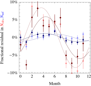
Figure 1: Left: Average number of citations $N_{\rm cit}$ (red) and of references $N_{\rm ref}$ (blue) of publications in high-energy physics in arXiv as function of time. Both show an annual modulation together with a trend on a slower, decennial, time-scale: $N_{\rm cit}$ is decreasing and $N_{\rm ref}$ is growing (smooth curves). Right: Monthly variation computed integrating over the years and subtracting the slow trend in two different ways: subtracting the discontinuous yearly averages (lighter red and blue) or their smooth averages (darker red and blue).

A different analysis procedure allows to search for a modulation over a slowly varying background without introducing an artificial modulation that biases the signal. The residuals are now computed by subtracting a smooth function that follows the average slow evolution of the background, rather than the discontinuous yearly averages. Such functions can be obtained, for example, as a 1^st or 2^nd order interpolation of the yearly averages. In this language the ‘dangerous’ procedure corresponds to subtracting a 0^th order discontinuous interpolation. The two possibilities are plotted in lighter/darker color in fig. 1. The right panel of fig. 1 shows the residuals computed following the two procedures. As expected, the two modulation residuals differ by a few $\%$, and their phase is shifted. The correct procedure shows that $N_{\rm cit}$ oscillates by about $5\%$ and that $N_{\rm ref}$ oscillates by about $1\%$; both peak around April. The ‘dangerous’ procedure incorrectly determines the modulation amplitudes and their phases.

3 The DAMA analysis: simulation

We now apply the above considerations to the DAMA analysis. The experiment is looking for an annual modulation in the rate of single-hit scintillation events in NaI crystals, as a possible signal of DM interactions with matter. The total rate is dominated by large backgrounds due to natural radioactivity of the detector and surrounding environment. As discussed above, a background that evolves slowly on a longer time-scale (say decennial) can simulate an annual modulation if the analysis is performed by subtracting yearly weighted averages. Since this is the procedure followed by the DAMA  collaboration, we study the possible impact of this observation on the results.

The cumulative total rates expressed in cpd/kg/keVee (where ‘ee’ stands for electron equivalent) have been presented as a function of the electron-equivalent recoil energy in three long-run phases in fig. 1 of [1], [3], and [5] for DAMA/NaI, DAMA/LIBRA Phase 1, and DAMA/LIBRA Phase 2, respectively. A change of the total rate between the three different phases is evident, and is due to improvements in the experimental setup causing an overall background reduction. However, its time dependence within a single data-taking phase is not provided by the collaboration, and cannot be inferred from these data alone.

The time dependence is reported for the residuals. In each of the three long-run phases, the DAMA residuals are derived from the measured rate of the single-hit scintillation events, after subtracting the time average of the rate over each cycle (of roughly yearly duration) such that “the weighted mean of the residuals must obviously be zero over one cycle” (see [1, 3, 4] and references therein). As discussed in the previous section, if the rate has the form of eq. (1) with a time-independent background $R_{0}(t)\equiv\mathcal{C}$, this procedure correctly subtracts the constant term. If instead $R_{0}(t)$ is slowly varying, the secular term contributes to the residuals, getting transformed to a sawtooth with periodicity equal to the duration of the DAMA cycles (injected because the analysis procedure is repeated quite regularly every year). The DAMA cycles start every year roughly around the beginning of September, so a growing background can appear like a modulated amplitude peaked at the beginning of June. On the contrary, the peak of the modulation would be around the beginning of December for a decreasing background.

We now show that a linearly growing background $R(t)$ without a periodic term can mimic a modulation that can look like the DAMA signal. We do so by first performing a Monte Carlo simulation, and next computing the residuals of the artificial data following the same procedure adopted by DAMA.

3.1 Monte Carlo simulation

The Monte Carlo simulation is done by employing a setup similar to the DAMA/LIBRA detector. In particular, for both Phase 1 and Phase 2 the total detector mass is taken to be $M=242.5$ kg (25 NaI crystals with a mass of 9.7 kg each) and we generate events in the energy window $(2\text{--}\,6)$ keVee such that $\Delta E=4$ keVee. The exposure of the 7 data-taking cycles in Phase 1 is 1.03 $\rm ton\cdot yr$, and their total duration is $\Delta T_{1}=2560$ days (table 1 of [4]); the exposure and total duration of the 6 data-taking cycles in Phase 2 are 1.13 $\rm ton\cdot yr$ and $\Delta T_{2}=2153$ days (table 1 of [5]). As a consequence, we assume a constant duty cycle efficiency $\zeta={\rm exposure}/(M\Delta T$) of $60\%$ and $80\%$ for Phase 1 and Phase 2, respectively.

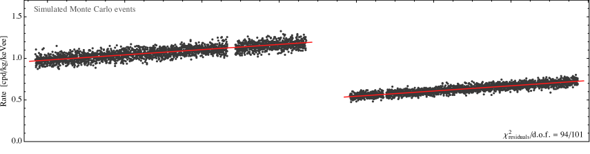
Figure 2: Upper: Monte Carlo events generated assuming no modulation, a slow linear growth in time, ${\cal B}=(0.01\,\pi/{\rm yr})\,{\rm cpd/kg/keVee}$, and the same cumulative rate as DAMA/LIBRA Phase 1 and 2. Lower: Residuals computed with respect to the smooth average are compatible with no modulation.

We generate a number of random events for each day following a Poisson distribution with mean

$$N(t)=\zeta M\Delta E\,R_{0}(t)\qquad\mbox{with }\qquad R_{0}(t)={\cal C}+{\cal B}t.$$ (9)

We assume that $R_{0}(t)$ grows linearly with time with a coefficient ${\cal B}={\cal A}\pi/\rm yr$, where ${\cal A}=0.01\,\rm cpd/kg/keVee$ is roughly the amplitude of the DAMA modulated signal. The constant ${\cal C}$ is chosen such that the time average of $R_{0}$ over the whole data-taking period is equal to the DAMA cumulative total rate in the $(2\text{--}6)$ keVee energy window: for Phase 1, $\langle R_{0}\rangle_{1}=1.03$ cpd/kg/keVee in an exposure of 0.53 $\rm ton\cdot yr$ [3]; for Phase 2, $\langle R_{0}\rangle_{2}=0.63$ cpd/kg/keVee in an exposure of 1.13 $\rm ton\cdot yr$ [5]. The upper panel of fig. 2 shows our simulated rate in cpd/kg/keVee as a function of time. The red lines represent the assumed backgrounds $R_{0}(t)$ in Phase 1 (on the left) and Phase 2 (on the right). Some short periods without data points are included consistently with the DAMA/LIBRA data acquisition.

We now compute the residuals of the simulated events following the procedure adopted by DAMA, i.e. subtracting the average event rate in each cycle. As expected we get a sawtooth up to statistical errors. A complication with respect to the ideal analysis of section 2 arises because the DAMA data-taking cycles have slightly irregular durations. The start and end dates of the 7 cycles of Phase 1 and the 6 cycles of Phase 2 can be found in table 1 of [4] and [5] respectively. Subtracting the average rate in the $k$-th cycle that lasts $\Delta T_{k}=t_{f,k}-t_{i,k}$ the residuals of eq. (9) follow the irregular sawtooth

$$\mathcal{S}(t)=\zeta M\Delta E\,S_{0}(t)\qquad\mbox{with }\qquad S_{0}(t)=\mathcal{B}\left(t-\frac{t_{i,k}+t_{f,k}}{2}\right)\quad\text{ for $t_{i,k}<t<t_{f,k}$}\,,$$ (10)

which is no longer a perfectly periodic function. We collect the residuals in 102 time bins of approximately 1.5 months each, adopting the same binning as the one used in the DAMA analysis. Fig. 3 illustrates the binned residuals expressed in cpd/kg/keVee. The errors are of the same order of the errors of the DAMA residuals in the $(2\text{--}\,6)$ keVee energy window.

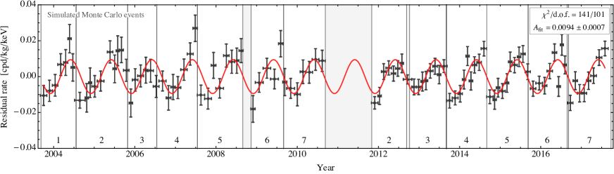
Figure 3: Residuals obtained from the simulated data of fig. 2 (black points) and computed within each data-taking cycle (vertical lines) following the DAMA procedure. The red curve shows the best fit to the simulated residuals with a DM cosine signal with a period of one year and peaked on June, 2nd. The zero-signal hypothesis is excluded with a significance of $12.7\,\sigma$ despite that no modulation was assumed in the simulated data.

This procedure results in something that looks like a cosine annual modulation. Unlike a true sinusoidal modulation, discontinuities are present between the various cycles. However, the binning procedure can partially wash out these discontinuities: if a time bin falls in two different cycles, as sometimes happens for the DAMA binning, the sawtooth will approximately average to zero over the bin, and the residual number of events in the bin will be small. Averaging the rate over 25 crystals with different efficiencies and duty cycles could also have an impact in this respect.

The consistency of the residual rate with a DM signal can be quantified by fitting the residual rate with a cosine with a period $T=1$ year, and peaked at $t_{\rm peak}=152.5$ days which corresponds to June, 2^nd. For our simulated Monte Carlo sample, the fit results in a cosine amplitude ${\cal A}=(0.0094\pm 0.0007)\,{\rm cpd/kg/keVee}$, consistent with the injected value of 0.01 cpd/kg/keVee. The goodness of the fit is given by $\chi^{2}=141$ for 101 degrees of freedom. The cosine signal is preferred over the zero-signal hypothesis at $12.7\,\sigma$, despite that no cosine modulation was present in the simulated data.

If instead the residuals are recomputed by subtracting the average rate as fitted to a linear function of time over the full data-taking period, the residuals (shown in the lower panel of fig. 2) are consistent with no modulation within one sigma ($\chi^{2}/{\rm d.o.f.}=94/101$).

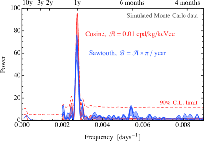
Figure 4: Left: Power spectra computed from Monte Carlo simulations assuming a sawtooth (blue line and band) and a cosine modulation (red band), with ${\cal A}={\cal B}\cdot{\rm yr}/\pi=0.01\,{\rm cpd/kg/keVee}$. The colored bands represent local $1\sigma$ intervals. The red dashed line shows the global 90% C.L. limit for a sinusoidal signal. Right: Power spectrum of the DAMA residuals (black) and annual rate (red) for Phase 1 and Phase 2 combined, taken from [5], together with the 90% C.L. allowed region (green) obtained from Monte Carlo simulations assuming a sawtooth with ${\cal B}=0.0219\pm 0.0026\,\,{\rm cpd/kg/keVee/yr}$ as in the combined DAMA/LIBRA best fit of Table 1.

In the left panel of fig. 4 we show the power spectrum (Lomb-Scargle periodogram as defined in [35]) corresponding to data simulated assuming a sawtooth as in fig. 2 (blue), and compare it to the power spectrum of a simulated annual cosine modulation (red) with ${\cal A}={\cal B}\cdot{\rm yr}/\pi=0.01$ cpd/kg/keVee. We computed the power spectrum following the procedure adopted by the DAMA collaboration in [5]. In the figure, the colored regions correspond to local $1\sigma$ intervals, computed by simulating 100 Monte Carlo samples; the red dashed line shows the global 90% C.L. allowed region, where all the peaks are expected to fall under the assumption of a sinusoidal signal of given amplitude (eq. (4) of [35]). We observe that:

• The power spectra at frequencies around and above 1/yr are obtained from the residuals computed within each cycle, and collected in bins of one day. The number of data points used to obtain the spectra is 4341 days, to match the value used in [5]. We see that both the sawtooth and the cosine produce comparable peaks at $\nu\approx 1/{\rm yr}$. The sawtooth contains extra Fourier modes with frequency $\nu\approx n/{\rm yr}$ and $n$ integer: the corresponding power is small because their amplitudes scale as $1/n$ (see eq. (5)), and the cycles are not exactly annual.

• Following [5], the power spectra at low frequencies below 1/yr are computed from average event rates in each (roughly annual) cycle. The main low-frequency peaks are due to the change in the total rate between Phase 1 and Phase 2; they do not have a statistically significant power because they are based on 7+7 time bins only.

• A power spectrum computed from daily total event rates was not considered in [3, 4, 5]. In the sawtooth simulation, it would exhibit significant power at low frequencies.

To summarize, a sawtooth modulation resulting from taking yearly residuals of a linearly growing background is statistically compatible with a sinusoidal modulation, given the available data. This conclusion is obtained both by fitting the explicit time series, and by performing a frequency analysis.

4 The DAMA analysis: experimental data

We now consider the real data collected by the DAMA experiment. The total rate as a function of time has not been explicitly published, and therefore we cannot directly know whether a secular evolution might have affected the determination of the modulation amplitude or its phase. We hence consider the published DAMA residuals, and show that their detailed time dependence is consistent even with the most extreme possibility: a sawtooth originating from a slowly growing background. A superposition of cosine and sawtooth, with the main contribution coming from the sinusoidal signal, is however preferred by a global fit.

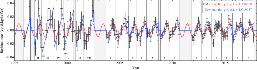
Figure 5: The black data points are the DAMA residuals in the $(2\text{--}\,6)$ ${\rm keVee}$ energy window, taken from [1, 5]. The curves are fits to a cosine annual modulation peaked on June, 2nd (red curve), as expected for a DM signal, and to the irregular sawtooth obtained from a continuously growing background (blue curve). The roughly annual data-taking cycles of DAMA/NaI, DAMA/LIBRA Phase 1, and DAMA/LIBRA Phase 2 are shown as vertical lines.

4.1 Fit to DAMA residuals

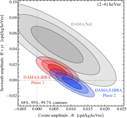
Figure 6: Fit of the DAMA residual rates to a sawtooth plus a cosine with period and phase as predicted by DM. Left: fit of residuals in the $(2\text{--}\,6)$ keVee energy window for DAMA/NaI (gray), DAMA/LIBRA Phase 1 (red) and Phase 2 (blue). Right: fit of residuals in the $(2\text{--}\,4)$ keVee energy window for DAMA/NaI (gray) and DAMA/LIBRA Phase 1 (red), and in the $(1\text{--}\,3)$ keVee energy window for DAMA/LIBRA Phase 2.

We again assume a linearly growing total rate as in eq. (3). This assumption is motivated by the amplitude of the observed modulation seeming constant over the Phase 1 and Phase 2 cycles, which requires a slow constant growth of the rate if the modulation is interpreted as a sawtooth. Furthermore, a constant growth is a good approximation if the time-scale of the secular evolution is long compared to the duration of the data-taking cycles. However, the time dependence of the background is unknown, and details of our analysis depend of course on it.

The experimental residual rates as a function of time in three different energy intervals are taken from [3], [4] and [5] for DAMA/NaI, DAMA/LIBRA Phase 1 and Phase 2 respectively. The residual rate in the $(2\text{--}6)$ keVee energy interval is extracted from [3, 5] and shown in fig. 5 as black points, together with the timespan of the 20 annual cycles of the experiment. We fit all these data points with the following two signal functions:

1. A cosine modulation ${\cal A}\cos[2\pi(t-t_{\rm peak})/T]$ with $T=1\,{\rm yr}$ and $t_{\rm peak}=$ June, 2^nd, as predicted for a DM-induced annual modulation signal;

2. The irregular sawtooth generated by a growing background $\mathcal{B}t$, taking into account the details of the DAMA cycles as in eq. (10).

In the fit we allow for two different values of the sawtooth amplitude: $\mathcal{B}_{\rm LIBRA}$ for the two phases of DAMA/LIBRA, and $\mathcal{B}_{\rm NaI}$ for DAMA/NaI, as both the experimental apparatus and the total mass of the crystals were different. The best-fit curves for the two cases are shown in fig. 5. We find that both the cosine and the sawtooth provide good fits to the data, as they have a $\chi^{2}$ per degree of freedom of order one. More precisely, the sawtooth fit has $\chi^{2}_{\rm saw}/{\rm d.o.f.}=137.1/137$, and the cosine fit has $\chi^{2}_{\cos}/{\rm d.o.f.}=118.8/138$.

The best-fit value for the cosine amplitude is in perfect agreement with the result reported by the DAMA collaboration, ${\cal A}=(0.0102\pm 0.0008)$ cpd/kg/keVee [5]. We get similar results when leaving the phase and period of the cosine free to vary. For the sawtooth, the best-fit values of the ${\cal B}$ coefficients are

$$\halign to=0.0pt{\@eqnsel\hskip\@centering$\displaystyle{#}$&\global\@eqcnt\@ne\hskip 2\arraycolsep\hfil${#}$\hfil& \global\@eqcnt\tw@\hskip 2\arraycolsep$\displaystyle{#}$\hfil&\llap{#}\cr 0.0pt plus 1000.0pt$\displaystyle{{\cal B}_{\rm NaI} &10.0pt\hfil${= (0.060\pm 0.009)\, {\rm cpd/kg/keVee/yr}\,,\\ {\cal B}_{\rm LIBRA} &10.0pt$\displaystyle{= (0.022\pm 0.003)\, {\rm cpd/kg/keVee/yr}\,, &\hbox to0.0pt{\hss(11)\cr}}}}}$$

for DAMA/NaI and DAMA/LIBRA, respectively, which correspond to a yearly growth of the total rate of a few percent. Allowing for different coefficients for Phase 1 and Phase 2, and even for each individual cycle, gives similar results.

The DAMA collaboration also reports residual rates in different energy windows. We perform a fit in all the energy intervals of DAMA/NaI, DAMA/LIBRA Phase 1 and Phase 2, and we find that both the cosine and the sawtooth give acceptable fits to the data. The two theoretical hypotheses result in similar $\chi^{2}/{\rm d.o.f.}$ in all cases, except for the higher energy bin of DAMA/LIBRA Phase 2 where a cosine is favoured. We also provide combined results with a single ${\cal B}$ for the three phases in the $(2\text{--}\,6)$ keVee energy interval where this is possible. The results of all our fits are summarized in table 1.

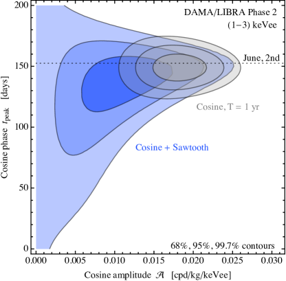
Figure 7: Left: Fit of the cosine amplitude and its phase to DAMA residuals, allowing for a sawtooth component (colored regions) or setting it to zero (gray regions). Left: combined fit in the $(2\text{--}\,6)$ keVee energy window. Right: fit of DAMA/LIBRA Phase 2 residuals in the $(1\text{--}\,3)$ keVee energy window.

Fitted	Fit to a cosine modulation		Fit to a secular variation
data	${\cal A}$ [cpd/kg/keVee]	$\chi^{2}_{\rm cos}/{\rm d.o.f.}$	${\cal B}$ [cpd/kg/keVee/yr]	$\chi^{2}_{\rm saw}/{\rm d.o.f.}$
DAMA/NaI
(2-4) keVee	$0.0214\pm 0.0046$	$36.3/36$	$0.0783\pm 0.0141$	$26.9/36$
(2-5) keVee	$0.0200\pm 0.0037$	$24.1/36$	$0.0605\pm 0.0113$	$24.7/36$
(2-6) keVee	$0.0178\pm 0.0031$	$36.9/36$	$0.0602\pm 0.0094$	$29.6/36$
LIBRA Phase I
(2-4) keVee	$0.0164\pm 0.0022$	$53.5/49$	$0.0452\pm 0.0059$	$51.9/49$
(2-5) keVee	$0.0120\pm 0.0016$	$42.8/49$	$0.0302\pm 0.0044$	$50.5/49$
(2-6) keVee	$0.0095\pm 0.0013$	$30.0/49$	$0.0249\pm 0.0035$	$33.6/49$
LIBRA Phase II
(1-3) keVee	$0.0182\pm 0.0023$	$61.2/51$	$0.0475\pm 0.0062$	$67.1/51$
(1-6) keVee	$0.0103\pm 0.0011$	$52.0/51$	$0.0230\pm 0.0029$	$83.7/51$
(2-6) keVee	$0.0093\pm 0.0011$	$44.8/51$	$0.0197\pm 0.0030$	$72.9/51$
LIBRA I and II
(2-6) keVee	$0.0094\pm 0.0008$	$74.8/101$	$0.0219\pm 0.0026$	$107.7/101$
DAMA combined
(2-6) keVee	$0.0100\pm 0.0008$	$118.8/138$	$0.0240\pm 0.0022$	$152.9/138$

Table 1: Best-fit values of the DM cosine amplitude ${\cal A}$ and the sawtooth coefficient ${\cal B}$ obtained by fitting the DAMA  residuals in different energy intervals, together with the corresponding $\chi^{2}/\text{d.o.f}$. Our fits of the cosine amplitudes agree with those reported by DAMA/LIBRA.

Keeping in mind that both the cosine and sawtooth provide acceptable fits to the data, we compare the two hypotheses by means of a likelihood ratio test. Indeed, when fitting data with many degrees of freedom, a likelihood-ratio test is a more powerful statistical indicator than the $\chi^{2}$ test. The two tests answer different questions: the $\chi^{2}$ compares the considered model to a generic model, such that all statistical fluctuations contribute. On the other hand, the $\Delta\chi^{2}$ compares two specific models such that only those statistical fluctuations that discriminate among the two models contribute. We perform a $\Delta\chi^{2}$ fit of the data to a generic superposition of a sawtooth plus a cosine. We fix the period of the cosine to one year, and its peak to June 2nd, as predicted for a DM-induced annual modulation signal, so that the only free parameter is the amplitude ${\cal A}$. The sawtooth also has one free parameter, the slope ${\cal B}$, since its phase and duration are fixed by the DAMA analysis choices. Fig. 6 shows the results of the fit as 68%, 95% and 99.7% allowed contours of ${\cal A}$ and ${\cal B}$. On the left we consider the $(2\text{--}\,6)$ keVee energy interval for the three phases of DAMA, while on the right we fit data in the lower energy window ($(2\,\text{--}\,4)$ keVee for both DAMA/NaI and DAMA/LIBRA Phase 1, and $(1\text{--}\,3)$ keVee for DAMA/LIBRA Phase 2). In the $(2\,\text{--}\,6)$ keVee interval the earlier DAMA/NaI data resemble more a sawtooth, while the more precise later Phase 2 data favour a cosine-dominated fit. Data in the lower energy interval are fitted equally well by both possibilities, a cosine or a secular variation.

Finally, we consider the cosine phase as an additional free parameter, still keeping the period fixed to one year, and quantify how much a possible sawtooth component relaxes the determination of the cosine amplitude and phase. In the left panel of fig. 7 we show the regions of ${\cal A}$ and $t_{\rm peak}$ preferred at 68%, 95% and 99.7% C.L. by the combined DAMA data-set in the $(2\text{--}\,6)$ keVee energy interval, both allowing for a free sawtooth component or setting it to zero. In the right panel we show the same but only for DAMA/LIBRA Phase 2 in the $(1\text{--}\,3)$ keVee energy interval. The best-fit regions assuming zero sawtooth (in gray) reproduce the results reported by DAMA (see e.g. fig. 15 of [5]). Allowing for a sawtooth component substantially affects the best fit regions. In particular, the phase of the cosine becomes more uncertain and can more significantly differ from the value characteristic of a DM signal, especially when fitting data at lower energy.

The DAMA collaboration analyzed the data by adopting two additional methods that are potentially relevant to indirectly clarify the time-dependence of the background. In [3, 4, 5] a frequency analysis of the residuals has been presented. In section 5 of [5] this result is complemented at frequencies below about 1/yr with a spectral analysis of the yearly averaged total rate. We have summarized relevant details of the procedure at the end of our section 3.1. We report in the right panel of fig. 4 the power spectrum of the combined DAMA/LIBRA Phase 1 and Phase 2 data, taken from [5], as black and red curves for the high and low frequencies, respectively. This power spectrum can be compared to what expected from a sawtooth or cosine annual modulation (shown in the left panel of fig. 4). The green region in the figure shows the global 90% C.L. upper limit obtained from Monte Carlo simulations, assuming a sawtooth with coefficient ${\cal B}$ as in our best fit to DAMA/LIBRA data of eq. (6). One can see that both the sawtooth and cosine hypotheses are compatible with the experimental data, reproducing the peak at a frequency of about 1/yr, without giving significant extra power at different frequencies.

In addition, a direct fit of signal plus background to the total event rate has been performed (see e.g. section 6 of [5]). In this case, however, the constant part of the background — $b_{jk}$ in the notation of [5] — is left free within each cycle [36]. This is effectively equivalent to fitting residuals, and does not avoid the issues discussed here.

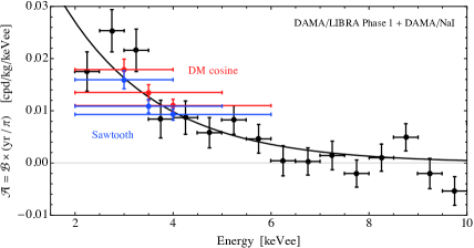
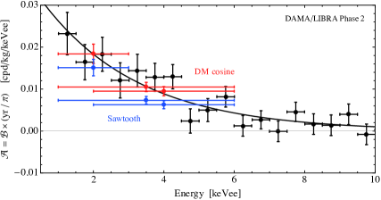
Figure 8: Energy dependence of the modulated signal observed by DAMA. The black points are the amplitudes of the cosine signal reported by DAMA in 0.5 keVee energy bins [5]; for comparison we also show the DM cosine amplitudes in the wider energy intervals discussed above (red points), and our best-fit values for a linearly growing background (blue points). The black curves fit the data assuming an exponential energy dependence. Left: Combination of DAMA/LIBRA Phase 1 and DAMA/NaI. Right: DAMA/LIBRA Phase 2.

4.2 Energy dependence of the secular variation

We now discuss the possible energy spectrum of the background rate $R_{0}(t)$ of eq. (3).

The DAMA collaboration provided the energy dependence of the cosine signal amplitude (see for example fig. 10 of [5]), showing separately the results for DAMA/LIBRA Phase 2, and for the combined DAMA/NaI and DAMA/LIBRA Phase 1. We report these data in the two panels of fig. 8 in black. The decrease of the rate with energy is approximately exponential as expected for DM-induced recoils. Above 6 keVee the modulated signal amplitude is compatible with zero.

We cannot repeat our fit over the whole energy range to extract the full energy dependence of the ${\cal B}$ coefficient, since the detailed time-dependence of the modulation is available only in the few energy bins discussed above. We however notice that in these three energy bins the values of ${\cal B}$ determined by fitting the data with a sawtooth, if compared with the cosine fit of DAMA, are close to the naïve expectation ${\cal B}\simeq{\cal A}\pi/T$ (see eq. (7)). This is shown in fig. 8, where the red points represent the amplitude of the modulated rate reported by DAMA, while the blue points correspond to our best-fit values of the sawtooth coefficient (rescaled by $\pi/\text{year})$. As one can see, the two sets of points are roughly compatible with each other, especially for the earlier experimental phases, and in the lower energy bins. We therefore use the detailed energy spectrum provided by DAMA (black points in the figure) as an approximate estimate of the energy dependence of ${\cal B}$.

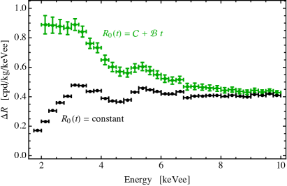
Figure 9: Left: Rate averaged over all data-taking time for DAMA/LIBRA Phase 2 (blue points), and for DAMA/LIBRA Phase 1 and DAMA/NaI combined (red points). Right: Difference in the total rate between the end of Phase 1 and the beginning of Phase 2, calculated assuming both a constant rate (black points), and a background that linearly grows with time (green points). In the latter case the values of ${\cal B}$ and ${\cal C}$ are chosen in order to reproduce the modulated signal and the cumulative rates; the errors come from the uncertainty in the residuals.

The constant part of the background ${\cal C}$ is determined by the energy spectrum of the total rate averaged over the whole data-taking period, shown in the left panel of fig. 9. These cumulative total rates differ between DAMA/LIBRA Phase 1 (red points taken from fig. 1 of [3]) and Phase 2 (blue points taken from fig. 1 of [5]), with a reduction of roughly a factor two between the two phases, most likely due to some improvement in the experimental setup. In the absence of a secular term in the background, this implies a change in the constant ${\cal C}$ which is trivially given by the difference of the cumulative rates. If a slowly growing term ${\cal B}t$ is present, by averaging over the data-taking period one gets that the variation of the total rate between the end of Phase 1 and the beginning of Phase 2 is given by

$$\Delta R\equiv R_{0}(t_{\rm 1,end})-R_{0}(t_{\rm 2,start})=R_{\rm 1}-R_{\rm 2}+\frac{{\cal B}}{2}(\Delta T_{\rm 1}+\Delta T_{\rm 2})\,,$$ (12)

where $R_{\rm 1,2}$, and $\Delta T_{\rm 1,2}$ are the average rate and total duration of the two phases. Since the energy spectra of $R_{\rm 1,2}$ and ${\cal B}$ are different, we report $\Delta R$ as a function of recoil energy in fig. 9 (right) for the two cases where a secular term is absent (black), or is fitted from the modulated signal (green). We do not give a physical explanation on the energy dependence of $\Delta R$.

Two comments are in order. First, the change in the averaged rate between the phases could in principle be entirely due to the secular term, if ${\cal B}<0$. A slowly decreasing background, however, would produce an oscillation peaked on December, in counterphase with the observed modulation. Second, the high-energy tails of the black points in fig. 9 (right) are approximately constant; one could therefore wonder whether the full difference could be explained by the energy dependence of the secular term ${\cal B}$ plus a constant shift $\Delta R$. This is indeed possible for a positive ${\cal B}$ with a spectrum peaked at low energies (below $\sim 5$ keVee), but its value in this case would be too small to completely reproduce the modulated signal with a sawtooth.

4.3 Possible slowly-varying backgrounds

A slow variation of the rate could, in principle, be produced by some signal or by some background. We here elaborate on the second possibility. The background in underground detectors in the keV energy range has spectral features and time behaviours that are poorly understood. We first consider possible slowly growing backgrounds, as their presence would give an apparent DAMA modulation peaked around June, as shown above. Various possible effects may create an increasing background, especially in a fixed energy window around few keV, as in the Region of Interest (RoI) of the DAMA experiment. We list a few generic examples of possible increasing backgrounds, not necessarily related to the specific case of study:

• Increase due to out-of-equilibrium physical effects. A classical example, although relevant at different energies, is the increase of the ²¹⁰Po, from a ²¹⁰Pb initial contamination in the transient phase after a broken equilibrium in the contamination chain Pb $\to$ Bi $\to$ Po. An increase of the backgrounds in NaI crystals could also arise from the diffusion of dirty materials from the surface into the bulk, as well as external gas cumulative contamination, as e.g. ²²²Rn. Other relevant out-of-equilibrium physical effects related to an increase of the backgrounds might be possible and can in principle be tested by dedicated analyses. A quantitative study of the backgrounds in NaI crystals has been reported in several papers by DAMA (see [37] and references therein) and more recently by other collaborations (e.g. [38]).

• Increase due to instrumental effects. These are related to the photo-multipliers (PMT) and electronics, and they are more difficult to isolate with respect to the previous ones. For example, helium gas permeating through PMT glass increases the after-pulse rate [39] creating fake low energy signals simulating the real scintillation. These are not easily rejectable through simple pulse shape discriminations, as suggested in [40] (although with completely different implications that we do not consider in this work). Another example is the possible increase of the electronic noise leaking in the acceptance region after pulse shape discrimination due to a generic loss of performance of the hardware.

• Apparent increase due to a general degradation of the detector resolution. This is potentially relevant in a fixed energy window close to the software threshold. Here the limit conditions of the reconstruction performances in terms of efficiency and reliability are usually reached.

We next consider the opposite scenario where the background is slowly decreasing with time. In this case the analysis procedure adopted by DAMA would transform the background into a sawtooth that mimics an annual modulation peaked around December, as discussed in section 2. Then, a decreasing background cannot explain the annual modulation reported by DAMA. However, the sawtooth could destructively interfere with additional periodic signals, in particular possibly shifting their phase, and a real DM signal would be distorted and attenuated.

A decrease of the total background rate could arise from different radioactive contaminants present in NaI crystals at the beginning of the data-taking as short and medium term cosmogenic activations or intrinsic out-of-equilibrium contaminants [6, 41, 10, 7, 42]. The most critical ones are those with a half-life $T_{1/2}$ of a few tens of years, comparable to the total time of data-taking, and an energy spectrum in the RoI of the detector. Examples of possible decreasing backgrounds in NaI crystals in the keV energy range include:

• Decay of relatively short-lived isotopes. For example, ¹⁰⁹Cd with $T_{1/2}=463$ days and ²²Na with $T_{1/2}=2.6$ yr. These contaminants are no longer relevant for DAMA because they have fully decayed after few years of data acquisition.

• Decay of medium-lived isotopes with a time-scale of order $\sim$10 yr. Typical contaminants that could be present at the beginning of data-taking are the cosmogenic ³H with $T_{1/2}=12.3$ yr, and ²¹⁰Pb with $T_{1/2}=22.3$ yr, which have about 40% and 16% of the energy spectrum falling in the RoI, respectively. In particular, the tritium has a $\beta$-spectrum peaked around 3 keV and with an endpoint of 18.6 keV. Being produced by cosmogenic activation, this contaminant is present in NaI crystals (grown in above-ground facilities) proportionally to the time exposure between their production and installation underground [43].

Let us stress that here we do not want to make any claim about the presence or absence of a given background, and even less to provide an explanation for the DAMA total rate. Since a careful reconstruction of the rate is strongly hampered by the poor knowledge of the background details, it would be extremely useful to directly check whether the DAMA background underwent a secular evolution. The COSINE (see e.g. [9]) and ANAIS (see e.g. [7]) experiments recently started data-taking using NaI crystals, and reported the total rates of each crystal as a function of time. The rates of these new experiments show, in their starting phase, a significant time-dependence.

5 Conclusions

The DAMA collaboration reported an annual modulation in the single-hit scintillation events that peaks around June, 2^nd, as predicted by a DM signal. The statistical significance of the DAMA signal is large, roughly $13\,\sigma$, such that the annual modulation could be in principle visible even by simply plotting the event rate binned as a function of time.

However, the DAMA collaboration reported residuals computed by subtracting the weighted average of its rate over cycles of roughly one year. This procedure can be dangerous, because a possible secular variation of the total rate would be transformed into a sawtooth with period coinciding with the duration of the DAMA analysis cycles. As a result, a slowly time-dependent rate, even if not oscillating, becomes a possible source of apparent modulation. Within the statistical accuracy, the modulation possibly produced by the procedure can resemble a cosine with period of one year. Since the data-analysis cycles usually start around September, the apparent cosine would peak at the beginning of June if the background slowly grows with time.

In section 3 we considered the most extreme possibility: a slowly and steadily growing background that fully reproduces the observed modulation amplitude in DAMA. By means of a Monte Carlo simulation, we have shown that the DM signal can be mimicked, within statistical errors, by a growth of the total rate on decennial time-scale. A rate that decreases with time, on the other hand, would suppress the oscillating signal.

The DAMA collaboration so far has not presented data about the time-dependence of its total rate, that can confirm or exclude the presence of a slowly changing background. We therefore tried to clarify the issue through the available indirect means in section 4.1. The detailed time dependence of the published residuals can be fitted by an irregular sawtooth with a $\chi^{2}/{\rm d.o.f.}\approx 1$, see fig. 5 and table 1. The available data are consistent with the modulation being interpreted as an artefact due to a yearly growth of the total rate of a few percent. A DM cosine provides a somehow better fit to parts of the data-set — specifically the higher energy bins of DAMA/LIBRA Phase 2 — therefore preferring a DM-like signal as a dominant explanation of the observed modulation. A time-dependent background rate would have an impact on the signal also in this case, since it would affect the extraction of the cosine amplitude and phase from the data, as shown in fig. 7. This effect can be important since the position of the sinusoid peak plays an important role in the interpretation of the modulation as a DM signal. A spectral analysis of the residuals and of the annual averaged rate is found to be consistent with a slow variation of the rate, as well as with a true annual modulation.

Finally, in section 4.2 we discussed the energy spectrum of the possible slowly-varying component of the rate, which must be peaked at low energy, and in section 4.3 we speculate about possible origins of such a background. We do not attempt at giving any realistic explanation of a possible time-dependence of the DAMA total rate; we rather just mention a few simple physical and instrumental effects that could produce a background that grows with time in the DAMA region of interest. It is worth mentioning that the ANAIS and COSINE experiments recently started data-taking with NaI crystals similar to the DAMA ones, and presented their rates as function of time, finding (in their initial phase) a sizeable time dependence [7, 9].

In conclusion, from the data available to us, we could not exclude the possibility that the cosine modulation claimed by DAMA is biased by a slow variation in the rate, possibly due to some background or signal. The most estreme possibility of no cosine modulation seems disfavoured, but we could not safely exclude it. More in general, a slowly increasing or decreasing rate would partially enhance or mask a true annual modulation, respectively.

The potential significance of our observation could, of course, be directly clarified by the measurement of the DAMA total rate as function of time. The absence of an appreciable variation of the rate over the time-scale of the experiment would exclude the relevance of the effects discussed in this paper for the DAMA analysis. A second possibility to test our observations would be to recompute the residual rate following a different procedure, such as subtracting the average background choosing cycles with different starting points or different durations. Even better, the above issues would be avoided by performing a detrend with continuous modelling of the possible time dependence of the background — such as a polynomial fit or interpolation — rather than a discontinuous average. Another possibility is to perform a signal processing in which, along with the original time series, both power spectrum and phase information are shown.

The direct detection of Dark Matter interactions in underground laboratories is one of the main challenges of contemporary particle physics. The observation of a DM signal would be an important discovery, so that any alternative interpretation needs to be explored with care. We therefore hope that an effort will be put by the experimental collaborations to settle the potential issues presented here.

Acknowledgements

This work was supported by ERC grant NEO-NAT and MIUR contracts 2017FMJFMW and 2017L5W2PT (PRIN). We thank Sabine Hossenfelder, Aldo Ianni, Marcello Messina and Tobias Mistele for discussions.

References

- [1] DAMA Collaboration, “Search for WIMP annual modulation signature: Results from DAMA/NaI-3 and DAMA/NaI-4 and the global combined analysis”, Phys. Lett. B480 (2000) 23 [\IfBeginWithBernabei:2000qi10.doi:Bernabei:2000qi\IfSubStrBernabei:2000qi:InSpire:Bernabei:2000qiarXiv:Bernabei:2000qi].
- [2] DAMA Collaboration, “Dark matter search”, Riv. Nuovo Cim. 26N1 (2003) 1 [\IfBeginWithastro-ph/030740310.doi:astro-ph/0307403\IfSubStrastro-ph/0307403:InSpire:astro-ph/0307403arXiv:astro-ph/0307403]. DAMA Collaboration, “Dark matter particles in the Galactic halo: Results and implications from DAMA/NaI”, Int. J. Mod. Phys. D13 (2005) 2127 [\IfBeginWithastro-ph/050141210.doi:astro-ph/0501412\IfSubStrastro-ph/0501412:InSpire:astro-ph/0501412arXiv:astro-ph/0501412].
- [3] DAMA Collaboration, “First results from DAMA/LIBRA and the combined results with DAMA/NaI”, Eur. Phys. J. C56 (2008) 333 [\IfBeginWith0804.274110.doi:0804.2741\IfSubStr0804.2741:InSpire:0804.2741arXiv:0804.2741].
- [4] DAMA Collaboration, “Final model independent result of DAMA/LIBRA-phase1”, Eur. Phys. J. C73 (2013) 2648 [\IfBeginWith1308.510910.doi:1308.5109\IfSubStr1308.5109:InSpire:1308.5109arXiv:1308.5109].
- [5] DAMA Collaboration, “First Model Independent Results from DAMA/LIBRA–Phase2”, Universe 4 (2019) 116 [\IfBeginWith1805.1048610.doi:1805.10486\IfSubStr1805.10486:InSpire:1805.10486arXiv:1805.10486].
- [6] ANAIS Collaboration, “Analysis of backgrounds for the ANAIS-112 dark matter experiment”, Eur. Phys. J. C79 (2019) 412 [\IfBeginWith1812.0137710.doi:1812.01377\IfSubStr1812.01377:InSpire:1812.01377arXiv:1812.01377].
- [7] ANAIS Collaboration, “First Results on Dark Matter Annual Modulation from the ANAIS-112 Experiment”, Phys. Rev. Lett. 123 (2019) 031301 [\IfBeginWith1903.0397310.doi:1903.03973\IfSubStr1903.03973:InSpire:1903.03973arXiv:1903.03973].
- [8] ANAIS Collaboration, “ANAIS-112 status: two years results on annual modulation” [\IfSubStr1910.13365:InSpire:1910.13365arXiv:1910.13365].
- [9] COSINE Collaboration, “Search for a Dark Matter-Induced Annual Modulation Signal in NaI(Tl) with the COSINE-100 Experiment”, Phys. Rev. Lett. 123 (2019) 031302 [\IfBeginWith1903.1009810.doi:1903.10098\IfSubStr1903.10098:InSpire:1903.10098arXiv:1903.10098].
- [10] COSINE Collaboration, “Study of cosmogenic radionuclides in the COSINE-100 NaI(Tl) detectors”, Astropart. Phys. 115 (2020-02) 102390 [\IfBeginWith1905.1286110.doi:1905.12861\IfSubStr1905.12861:InSpire:1905.12861arXiv:1905.12861].
- [11] COSINE Collaboration, “Comparison between DAMA/LIBRA and COSINE-100 in the light of Quenching Factors”, JCAP 1911 (2019) 008 [\IfBeginWith1907.0496310.doi:1907.04963\IfSubStr1907.04963:InSpire:1907.04963arXiv:1907.04963].
- [12] G. Tomar, S. Kang, S. Scopel, J-H. Yoon, “Is a WIMP explanation of the DAMA modulation effect still viable?” [\IfSubStr1911.12601:InSpire:1911.12601arXiv:1911.12601].
- [13] Particle Data Group, Phys. Rev. D 98 (2018) 030001.
- [14] P. Ullio, M. Kamionkowski, P. Vogel, “Spin dependent WIMPs in DAMA?”, JHEP 0107 (2000) 044 [\IfBeginWithhep-ph/001003610.doi:hep-ph/0010036\IfSubStrhep-ph/0010036:InSpire:hep-ph/0010036arXiv:hep-ph/0010036].
- [15] D. Tucker-Smith, N. Weiner, “Inelastic dark matter”, Phys. Rev. D64 (2001) 043502 [\IfBeginWithhep-ph/010113810.doi:hep-ph/0101138\IfSubStrhep-ph/0101138:InSpire:hep-ph/0101138arXiv:hep-ph/0101138].
- [16] M. Fairbairn, T. Schwetz, “Spin-independent elastic WIMP scattering and the DAMA annual modulation signal”, JCAP 0901 (2008) 037 [\IfBeginWith0808.070410.doi:0808.0704\IfSubStr0808.0704:InSpire:0808.0704arXiv:0808.0704].
- [17] J. Kopp, T. Schwetz, J. Zupan, “Global interpretation of direct Dark Matter searches after CDMS-II results”, JCAP 1002 (2009) 014 [\IfBeginWith0912.426410.doi:0912.4264\IfSubStr0912.4264:InSpire:0912.4264arXiv:0912.4264].
- [18] M. Farina, D. Pappadopulo, A. Strumia, T. Volansky, “Can CoGeNT and DAMA Modulations Be Due to Dark Matter?”, JCAP 1111 (2011) 010 [\IfBeginWith1107.071510.doi:1107.0715\IfSubStr1107.0715:InSpire:1107.0715arXiv:1107.0715].
- [19] N. Fornengo, P. Panci, M. Regis, “Long-Range Forces in Direct Dark Matter Searches”, Phys. Rev. D84 (2011) 115002 [\IfBeginWith1108.466110.doi:1108.4661\IfSubStr1108.4661:InSpire:1108.4661arXiv:1108.4661].
- [20] K. Blum, “DAMA vs. the annually modulated muon background” [\IfSubStr1110.0857:InSpire:1110.0857arXiv:1110.0857].
- [21] E. Del Nobile, C. Kouvaris, P. Panci, F. Sannino, J. Virkajarvi, “Light Magnetic Dark Matter in Direct Detection Searches”, JCAP 1208 (2012) 010 [\IfBeginWith1203.665210.doi:1203.6652\IfSubStr1203.6652:InSpire:1203.6652arXiv:1203.6652].
- [22] P. Panci, “New Directions in Direct Dark Matter Searches”, Adv. High Energy Phys. 2014 (2014) 681312 [\IfBeginWith1402.150710.doi:1402.1507\IfSubStr1402.1507:InSpire:1402.1507arXiv:1402.1507].
- [23] C. Arina, E. Del Nobile, P. Panci, “Dark Matter with Pseudoscalar-Mediated Interactions Explains the DAMA Signal and the Galactic Center Excess”, Phys. Rev. Lett. 114 (2015) 011301 [\IfBeginWith1406.554210.doi:1406.5542\IfSubStr1406.5542:InSpire:1406.5542arXiv:1406.5542].
- [24] R. Catena, A. Ibarra, S. Wild, “DAMA confronts null searches in the effective theory of dark matter-nucleon interactions”, JCAP 1605 (2016) 039 [\IfBeginWith1602.0407410.doi:1602.04074\IfSubStr1602.04074:InSpire:1602.04074arXiv:1602.04074].
- [25] P. Gondolo, S. Scopel, “Halo-independent determination of the unmodulated WIMP signal in DAMA: the isotropic case”, JCAP 1709 (2017) 032 [\IfBeginWith1703.0894210.doi:1703.08942\IfSubStr1703.08942:InSpire:1703.08942arXiv:1703.08942].
- [26] J. Herrero-Garcia, A. Scaffidi, M. White, A.G. Williams, “Time-dependent rate of multicomponent dark matter: Reproducing the DAMA/LIBRA phase-2 results”, Phys. Rev. D98 (2018) 123007 [\IfBeginWith1804.0843710.doi:1804.08437\IfSubStr1804.08437:InSpire:1804.08437arXiv:1804.08437].
- [27] B.M. Roberts, V.V. Flambaum, “Electron-interacting dark matter: Implications from DAMA/LIBRA-phase2 and prospects for liquid xenon detectors and NaI detectors”, Phys. Rev. D100 (2019) 063017 [\IfBeginWith1904.0712710.doi:1904.07127\IfSubStr1904.07127:InSpire:1904.07127arXiv:1904.07127].
- [28] S. Kang, S. Scopel, G. Tomar, “A DAMA/Libra-phase2 analysis in terms of WIMP-quark and WIMP-gluon effective interactions up to dimension seven” [\IfSubStr1910.11569:InSpire:1910.11569arXiv:1910.11569].
- [29] V.A. Kudryavtsev, M. Robinson, N.J.C. Spooner, “The expected background spectrum in NaI dark matter detectors and the DAMA result”, Astropart. Phys. 33 (2009) 91 [\IfBeginWith0912.298310.doi:0912.2983\IfSubStr0912.2983:InSpire:0912.2983arXiv:0912.2983].
- [30] J.P. Ralston, “One Model Explains DAMA/LIBRA, CoGENT, CDMS, and XENON” [\IfSubStr1006.5255:InSpire:1006.5255arXiv:1006.5255].
- [31] R.W. Schnee, “Introduction to dark matter experiments” [\IfSubStr1101.5205:InSpire:1101.5205arXiv:1101.5205].
- [32] D. Nygren, “A testable conventional hypothesis for the DAMA-LIBRA annual modulation” [\IfSubStr1102.0815:InSpire:1102.0815arXiv:1102.0815].
- [33] P.W. Graham, D.E. Kaplan, S. Rajendran, “Cosmological Relaxation of the Electroweak Scale”, Phys. Rev. Lett. 115 (2015) 221801 [\IfBeginWith1504.0755110.doi:1504.07551\IfSubStr1504.07551:InSpire:1504.07551arXiv:1504.07551].
- [34] High-Energy Physics Literature InSpire Database. A. Holtkamp, S. Mele, T. Simko, and T. Smith (InSpire collaboration), “Inspire: Realizing the dream of a global digital library in high-energy physics”, 2010. See also “INSPIRE-HEP Documentation” (2018) by the InSpire-HEP Collaboration.
- [35] G. Ranucci, M. Rovere, “Periodogram and likelihood periodicity search in the SNO solar neutrino data”, Phys. Rev. D75 (2006) 013010 [\IfBeginWithhep-ph/060521210.doi:hep-ph/0605212\IfSubStrhep-ph/0605212:InSpire:hep-ph/0605212arXiv:hep-ph/0605212].
- [36] Private communication.
- [37] DAMA Collaboration, “Dark Matter investigation by DAMA at Gran Sasso”, Int. J. Mod. Phys. A28 (2013) 1330022 [\IfBeginWith1306.141110.doi:1306.1411\IfSubStr1306.1411:InSpire:1306.1411arXiv:1306.1411].
- [38] G. Adhikari et al., “Understanding NaI(Tl) crystal background for dark matter searches”, Eur. Phys. J. C77 (2017) 437 [\IfBeginWith1703.0198210.doi:1703.01982\IfSubStr1703.01982:InSpire:1703.01982arXiv:1703.01982].
- [39] “Photomultiplier tubes”, Hammatsu Photonics K.K., 2007.
- [40] D. Ferenc, D. Ferenc Šegedin, I. Ferenc Šegedin, M. Šegedin Ferenc, “Helium Migration through Photomultiplier Tubes – The Probable Cause of the DAMA Seasonal Variation Effect” [\IfSubStr1901.02139:InSpire:1901.02139arXiv:1901.02139].
- [41] ANAIS Collaboration, “Performance of ANAIS-112 experiment after the first year of data taking”, Eur. Phys. J. C79 (2019) 228 [\IfBeginWith1812.0147210.doi:1812.01472\IfSubStr1812.01472:InSpire:1812.01472arXiv:1812.01472].
- [42] B. Suerfu, M. Wada, W. Peloso, M. Souza, F. Calaprice, J. Tower, G. Ciampi, “Growth of Ultra-high Purity NaI(Tl) Crystal for Dark Matter Searches” [\IfSubStr1910.03782:InSpire:1910.03782arXiv:1910.03782].
- [43] J. Amare et al., “Cosmogenic production of tritium in dark matter detectors”, Astropart. Phys. 97 (2018-01) 96 [\IfBeginWith1706.0581810.doi:1706.05818\IfSubStr1706.05818:InSpire:1706.05818arXiv:1706.05818].