Choice Set Optimization Under Discrete Choice Models of Group Decisions

Abstract

The way that people make choices or exhibit preferences can be strongly affected by the set of available alternatives, often called the choice set. Furthermore, there are usually heterogeneous preferences, either at an individual level within small groups or within sub-populations of large groups. Given the availability of choice data, there are now many models that capture this behavior in order to make effective predictions—however, there is little work in understanding how directly changing the choice set can be used to influence the preferences of a collection of decision-makers. Here, we use discrete choice modeling to develop an optimization framework of such interventions for several problems of group influence, namely maximizing agreement or disagreement and promoting a particular choice. We show that these problems are NP-hard in general, but imposing restrictions reveals a fundamental boundary: promoting a choice can be easier than encouraging consensus or sowing discord. We design approximation algorithms for the hard problems and show that they work well on real-world choice data.

1 Context effects and optimizing choice sets

Choosing from a set of alternatives is one of the most important actions people take, and choices determine the composition of governments, the success of corporations, and the formation of social connections. For these reasons, choice models have received significant attention in the fields of economics (Train, 2009), psychology (Tversky & Kahneman, 1981), and, as human-generated data has become increasingly available online, computer science (Overgoor et al., 2019; Seshadri et al., 2019; Rosenfeld et al., 2020). In many cases, it is important that people have heterogeneous preferences; for example, people living in different parts of a town might prefer different government policies.

Much of the computational work on choice has been devoted to fitting models for predicting future choices. In addition to prediction, another area of interest is determining effective interventions to influence choice—advertising and political campaigning are prime examples. In heterogeneous groups, the goal might be to encourage consensus (Amir et al., 2015), or, for an ill-intentioned adversary, to sow discord, e.g., amongst political parties (Rosenberg et al., 2020).

One particular method of influence is introducing new alternatives or options. While early economic models assume that alternatives are irrelevant to the relative ranking of options (Luce, 1959; McFadden, 1974), experimental work has consistently found that new alternatives have strong effects on our choices (Huber et al., 1982; Simonson & Tversky, 1992; Shafir et al., 1993; Trueblood et al., 2013). These effects are often called context effects or choice set effects. A well-known example is the compromise effect (Simonson, 1989), which describes how people often prefer a middle ground (e.g., the middle-priced wine). Direct measurements on choice data have also revealed choice set effects in several domains (Benson et al., 2016; Seshadri et al., 2019).

Here, we pose adding new alternatives as a discrete optimization problem for influencing a collection of decision makers, such as the inhabitants of a city or the visitors to a website. To this end, we consider various models for how someone makes a choice from a given set of alternatives, where the model parameters can be readily estimated from data. In our setup, everyone has a base set of alternatives from which they make a choice, and the goal is to find a set of additional alternatives to optimize some function of the group’s joint preferences on the base set. We specifically analyze three objectives: (i) agreement in preferences amongst the group; (ii) disagreement in preferences amongst the group; and (iii) promotion of a particular item (decision).

We use the framework of discrete choice (Train, 2009) to probabilistically model a person’s choice from a given set of items, called the choice set. These models are parameterized for individual preferences, and when fitting parameters from data, preferences are commonly aggregated at the level of a sub-population of individuals. Discrete choice models such as the multinomial logit and elimination-by-aspects have played a central role in behavioral economics for several decades with diverse applications, including forest management (Hanley et al., 1998), social networks formation (Overgoor et al., 2019), and marketing campaigns (Fader & McAlister, 1990). More recently, new choice data and algorithms have spurred machine learning research on models for choice set effects (Ragain & Ugander, 2016; Chierichetti et al., 2018b; Seshadri et al., 2019; Pfannschmidt et al., 2019; Rosenfeld et al., 2020; Bower & Balzano, 2020).

We provide the relevant background on discrete choice models in Section 2. From this, we formally define and analyze three choice set optimization problems—Agreement, Disagreement, and Promotion—and analyze them under four discrete choice models: multinomial logit (McFadden, 1974), the context dependent random utility model (Seshadri et al., 2019), nested logit (McFadden, 1978), and elimination-by-aspects (Tversky, 1972). We first prove that the choice set optimization problems are NP-hard in general for these models. After, we identify natural restrictions of the problems under which they become tractable. These restrictions reveal a fundamental boundary: promoting a particular item within a group is easier than minimizing or maximizing consensus. More specifically, we show that restricting the choice models can make Promotion tractable while leaving Agreement and Disagreement NP-hard, indicating that the interaction between individuals introduces significant complexity to choice set optimization.

After this, we provide efficient approximation algorithms with guarantees for all three problems under several choice models, and we validate our algorithms on choice data. Model parameters are learned for different types of individuals based on features (e.g., where someone lives). From these learned models, we apply our algorithms to optimize group-level preferences. Our algorithms outperform a natural baseline on real-world data coming from transportation choices, insurance policy purchases, and online shopping.

1.1 Related work

Our work fits within recent interest from computer science and machine learning on discrete choice models in general and choice set effects in particular. For example, choice set effects abundant in online data has led to richer data models (Ieong et al., 2012; Chen & Joachims, 2016; Ragain & Ugander, 2016; Seshadri et al., 2019; Makhijani & Ugander, 2019; Rosenfeld et al., 2020; Bower & Balzano, 2020), new methods for testing the presence of choice set effects (Benson et al., 2016; Seshadri et al., 2019; Seshadri & Ugander, 2019), and new learning algorithms (Kleinberg et al., 2017; Chierichetti et al., 2018b). More broadly, there are efforts on learning algorithms for multinomial logit mixtures (Oh & Shah, 2014; Ammar et al., 2014; Kallus & Udell, 2016; Zhao & Xia, 2019), Plackett-Luce models (Maystre & Grossglauser, 2015; Zhao et al., 2016), and other random utility models (Oh et al., 2015; Chierichetti et al., 2018a; Benson et al., 2018).

One of our optimization problems is maximizing group agreement by introducing new alternatives. This is motivated in part by how additional context can sway opinion on controversial topics (Munson et al., 2013; Liao & Fu, 2014; Graells-Garrido et al., 2014). There are also related algorithms for decreasing polarization in social networks (Garimella et al., 2017; Matakos et al., 2017; Chen et al., 2018; Musco et al., 2018), although we have no explicit network and adopt a choice-theoretic framework.

Our choice set optimization framework is similar to assortment optimization in operations research, where the goal is find the optimal set of products to offer in order to maximize revenue (Talluri & Van Ryzin, 2004). Discrete choice models are extensively used in this line of research, including the multinomial logit (Rusmevichientong et al., 2010, 2014) and nested logit (Gallego & Topaloglu, 2014; Davis et al., 2014) models. We instead focus our attention primarily on optimizing agreement among individuals, which has not been explored in traditional revenue-focused assortment optimization.

Finally, our problems relate to group decision-making. In psychology, introducing new shared information is critical for group decisions (Stasser & Titus, 1985; Lu et al., 2012). In computer science, the complexity of group Bayesian reasoning is a concern (Hązła et al., 2017, 2019).

2 Background and preliminaries

We first introduce the discrete choice models that we analyze. In the setting we explore, one or more individuals make a (possibly random) choice of a single item (or alternative) from a finite set of items called a choice set. We use $\mathcal{U}$ to denote the universe of items and $C\subseteq\mathcal{U}$ the choice set. Thus, given $C$, an individual chooses some item $x\in C$.

Given $C$, a discrete choice model provides a probability for choosing each item $x\in C$. We analyze four broad discrete choice models that are all random utility models (RUMs), which derive from economic rationality. In a RUM, an individual observes a random utility for each item $x\in C$ and then chooses the one with the largest utility. We model each individual’s choices through the same RUM but with possibly different parameters to capture preference heterogeneity. In this sense, we have a mixture model.

Choice data typically contains many observations from various choice sets. We occasionally have data specific enough to model the choices of a particular individual, but often only one choice is recorded per person, making accurate preference learning impossible at that scale. Thus, we instead model the heterogeneous preferences of sub-populations or categories of individuals. For convenience, we still use “individual” or “person” when referring to components of a mixed population, since we can treat each component as a decision-making agent with its own preferences. In contrast, we use the term “group” to refer to the entire population. We use $A$ to denote the set of individuals (in the broad sense above), and $a\in A$ indexes model parameters.

The parameters of the RUMs we analyze can be inferred from data, and our theoretical results and algorithms assume that we have learned these parameters. Our analysis focuses on how the probability of selecting an item $x$ from a choice set $C$ changes as we add new alternative items from $\overline{C}=\mathcal{U}\setminus C$ to the choice set.

We let $n=|A|$, $k=|C|$, and $m=|\overline{C}|$ for notation. We mostly use $n=2$, which is sufficient for hardness proofs.

Multinomial logit (MNL).  The multinomial logit (MNL) model (McFadden, 1974) is the workhorse of discrete choice theory. In MNL, an individual $a$’s preferences are encoded by a true utility $u_{a}(x)$ for every item $x\in\mathcal{U}$. The observations are noisy random utilities $\tilde{u}_{a}(x)=u_{a}(x)+\varepsilon$, where $\varepsilon$ follows a Gumbel distribution. Under this model, the probability that individual $a$ picks item $x$ from choice set $C$ (i.e., $x=\operatorname*{arg\,max}_{y\in C}\tilde{u}_{a}(y)$) is the softmax over item utilities:

$$\Pr(a\leftarrow x\mid C)=\frac{e^{u_{a}(x)}}{\sum_{y\in C}e^{u_{a}(y)}}.$$ (1)

We use the term exp-utility for terms like $e^{u_{a}(x)}$. The utility of an item is often parameterized as a function of features of the item in order to generalize to unseen data. For example, a linear function is an additive utility model (Tversky & Simonson, 1993) and looks like logistic regression. In our analysis, we work directly with the utilities.

The MNL satisfies independence of irrelevant alternatives (IIA) (Luce, 1959), the property that for any two choice sets $C,D$ and two items $x,y\in C\cap D$: $\frac{\Pr(a\leftarrow x\mid C)}{\Pr(a\leftarrow y\mid C)}=\frac{\Pr(a\leftarrow x\mid D)}{\Pr(a\leftarrow y\mid D)}$. In other words, the choice set has no effect on $a$’s relative probability of choosing $x$ or $y$. Although IIA is intuitively pleasing, behavioral experiments show that it is often violated in practice (Huber et al., 1982; Simonson & Tversky, 1992). Thus, there are many models that account for IIA violations, including the other ones we analyze.

Context-dependent random utility model (CDM).  The CDM (Seshadri et al., 2019) is an extension of MNL that can model IIA violations. The core idea is to approximate choice set effects by the effect of each item’s presence on the utilities of the other items. For instance, a diner’s preference for a ribeye steak may decrease relative to a fish option if filet mignon is also available. Formally, each item $z$ exerts a pull on $a$’s utility from $x$, which we denote $p_{a}(z,x)$. The CDM then resembles the MNL with utilities $u_{a}(x\mid C)=u_{a}(x)+\sum_{z\in C}p_{a}(z,x)$. This leads to choice probabilities that are a softmax over the context-dependent utilities:

$$\Pr(a\leftarrow x\mid C)=\frac{e^{u_{a}(x\mid C)}}{\sum_{y\in C}e^{u_{a}(y\mid C)}}.$$ (2)

Nested logit (NL).  The nested logit (NL) model (McFadden, 1978) instead accounts for choice set effects by grouping similar items into nests that people choose between successively. For example, a diner may first choose between a vegetarian, fish, or steak meal and then select a particular dish. NL can be derived by introducing correlation between the random utility noise $\varepsilon$ in MNL; here, we instead consider a generalized tree-based version of the model.

The (generalized) NL model for an individual $a$ consists of a tree $T_{a}$ with a leaf for each item in $\mathcal{U}$, where the internal nodes represent categories of items. Rather than having a utility only on items, each person $a$ also has utilities $u_{a}(v)$ on all nodes $v\in T_{a}$ (except the root). Given a choice set $C$, let $T_{a}(C)$ be the subtree of $T_{a}$ induced by $C$ and all ancestors of $C$. To choose an item from $C$, $a$ starts at the root and repeatedly picks between the children of the current node according to the MNL model until reaching a leaf.

Elimination-by-aspects (EBA).  While the previous models are based on MNL, the elimination-by-aspects (EBA) model (Tversky, 1972) has a different structure. In EBA, each item $x$ has a set of aspects $x^{\prime}$ representing properties of the item, and person $a$ has a utility $u_{a}(\chi)>0$ on each aspect $\chi$. An item is chosen by repeatedly picking an aspect with probability proportional to its utility and eliminating all items that do not have that aspect until only one item remains (or, if all remaining items have the same aspects, the choice is made uniformly at random). For example, a diner may first eliminate items that are too expensive, then disregard meat options, and finally look for dishes with pasta before choosing mushroom ravioli. Formally, let $C^{\prime}=\bigcup_{x\in C}x^{\prime}$ be the set of aspects of items in $C$ and let $C^{0}=\bigcap_{x\in C}x^{\prime}$ be the aspects shared by all items in $C$. Additionally, let $C_{\chi}=\{x\in C\mid\chi\in x^{\prime}\}$. The probability that individual $a$ picks item $x$ from choice set $C$ is recursively defined as

$$\Pr(a\leftarrow x\mid C)=\frac{\sum_{\chi\in x^{\prime}\setminus C^{0}}u_{a}(\chi)\Pr(a\leftarrow x\mid C_{\chi})}{\sum_{\psi\in C^{\prime}\setminus C^{0}}u_{a}(\psi)}.$$ (3)

If all remaining items have the same aspects ($C^{\prime}=C^{0}$), the denominator is zero, and $\Pr(a\leftarrow x\mid C)=\frac{1}{|C|}$ in that case.

Encoding MNLs in other models.  Although the three models with context effects appear quite different, they all subsume the MNL model. Thus, if we prove a problem hard under MNL, then it is hard under all four models.

Lemma 1.

The MNL model is a special case of the CDM, NL, and EBA models.

Proof.

Let $\mathcal{M}$ be an MNL model. For the CDM, use the utilities from $\mathcal{M}$ and set all pulls to 0. For NL, make all items children of $T_{a}$’s root and use the utilities from $\mathcal{M}$. Lastly, for EBA, assign a unique aspect $\chi_{x}$ to each item $x\in\mathcal{U}$ with utility $u_{a}(\chi_{x})=e^{u_{a}(x)}$. Following (3),

$$\Pr(a\leftarrow x\mid C)=\frac{u_{a}(\chi_{x})\Pr(a\leftarrow x\mid C_{\chi_{x}})}{\sum_{\psi\in C^{\prime}\setminus C^{0}}u_{a}(\psi)}.$$

Since $C_{\chi_{x}}=\{x\}$, $\Pr(a\leftarrow x\mid C_{\chi_{x}})=1$ and thus $\Pr(a\leftarrow x\mid C)\propto u_{a}(\chi_{x})=e^{u_{a}(x)}$, matching the MNL $\mathcal{M}$. ∎

3 Choice set optimization problems

By introducing new alternatives to the choice set $C$, we can modify the relationships amongst individual preferences, resulting in different dynamics at the collective level. Similar ideas are well-studied in voting models, e.g., introducing alternatives to change winners selected by Borda count (Easley & Kleinberg, 2010). Here, we study how to optimize choice sets for various group-level objectives, measured in terms of individual choice probabilities coming from discrete choice models.

Agreement and Disagreement.  Since we are modeling the preferences of a collection of decision-makers, one important metric is the amount of disagreement (conversely, agreement) about which item to select. Given a set of alternatives $Z\subseteq\overline{C}$ we might introduce, we quantify the disagreement this would induce as the sum of all pairwise differences between individual choice probabilities over $C$:

$$D(Z)=\smashoperator[]{\sum_{\{a,b\}\subseteq A,x\in C}^{}}|\Pr(a\leftarrow x\mid C\cup Z)-\Pr(b\leftarrow x\mid C\cup Z)|.$$ (4)

Here, we care about the disagreement on the original choice set $C$ that results from preferences over the new choice set $C\cup Z$. In this setup, $C$ could represent core options (e.g., two major health care policies under deliberation) and $Z$ additional alternatives designed to sway opinions.

Concretely, we study the following problem: given $A,C,\overline{C}$, and a choice model, minimize (or maximize) $D(Z)$ over $Z\subseteq\overline{C}$. We call the minimization problem Agreement and the maximization problem Disagreement. Agreement has applications in encouraging consensus, while Disagreement yields insight into how susceptible a group may be to an adversary who wishes to increase conflict. Another potential application for Disagreement is to enrich the diversity of preferences present in a group.

Promotion.  Promoting an item is another natural objective, which is of considerable interest in online advertising and content recommendation. Given $A,C,\overline{C}$, a choice model, and a target item $x^{*}\in C$, the Promotion problem is to find the set of alternatives $Z\subseteq\overline{C}$ whose introduction maximizes the number of individuals whose “favorite” item in $C$ is $x^{*}$. Formally, this means maximizing the number of individuals $a\in A$ for whom $\Pr(a\leftarrow x^{*}\mid C\cup Z)>\Pr(a\leftarrow x\mid C\cup Z)$, $x\in C$, $x\neq x^{*}$. This also has applications in voting, where questions about the influence of new candidates constantly arise.

One of our contributions in this paper is showing that promotion can be easier (in a computational complexity sense) than agreement or disagreement optimization.

4 Hardness results

We now characterize the computational complexity of Agreement, Disagreement, and Promotion under the four discrete choice models. We first show that Agreement and Disagreement are NP-hard under all four models and that Promotion is NP-hard under the three models with context effects. After, we prove that imposing additional restrictions on these discrete choice models can make Promotion tractable while leaving Agreement and Disagreement NP-hard. The parameters of some choice models have extra degrees of freedom, e.g., MNL has additive-shift-invariant utilities. For inference, we use a standard form (e.g., sum of utilities equals zero). For ease of analysis, we do not use such standard forms, but the choice probabilities remain unambiguous.

4.1 Agreement

Although the MNL model does not have any context effects, introducing alternatives to the choice set can still affect the relative preferences of two different individuals. In particular, introducing alternatives can impact disagreement in a sufficiently complex way to make identifying the optimal set of alternatives computationally hard. Our proof of Theorem 1 uses a very simple MNL in the reduction, with only two individuals and two items in $C$, where the two individuals have exactly the same utilities on alternatives. In other words, even when individuals agree about new alternatives, encouraging them to agree over the choice set is hard.

Theorem 1.

In the MNL model, Agreement is NP-hard, even with just two items in $C$ and two individuals that have identical utilities on items in $\overline{C}$.

Proof.

By reduction from Partition, an NP-complete problem (Karp, 1972). Let $S$ be the set of integers we wish to partition into two subsets with equal sum. We construct an instance of Disagreement with $A=\{a,b\}$, $C=\{x,y\}$, $\overline{C}=S$ (abusing notation to identify alternatives with the Partition integers). Let $t=\frac{1}{2}\sum_{z\in S}z$. Define the utilities as: $u_{a}(x)=\log t$, $u_{b}(x)=\log 3t$, $u_{a}(y)=\log t$, $u_{b}(y)=\log 2t$, and $u_{a}(z)=u_{b}(z)=\log z$ for all $z\in\overline{C}$. The disagreement induced by a set of alternatives $Z\subseteq\overline{C}$ is characterized by its sum of exp-utility $s_{Z}=\sum_{z\in Z}z$:

$$D(Z)=\left|\frac{t}{2t+s_{Z}}-\frac{3t}{5t+s_{Z}}\right|+\left|\frac{t}{2t+s_{Z}}-\frac{2t}{5t+s_{Z}}\right|.$$

The total exp-utility of all items in $\overline{C}$ is $2t$. On the interval $[0,2t]$, $D(Z)$ is minimized at $s_{Z}=t$ (Fig. 1, left). Thus, if we could efficiently find the set $Z$ minimizing $D(Z)$, then we could efficiently solve Partition. ∎

From Lemma 1, the other models we consider can all encode any MNL instance, which leads to the following corollary.

Corollary 1.

Agreement is NP-hard in the CDM, NL, and EBA models.

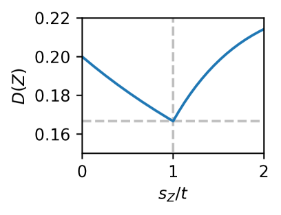
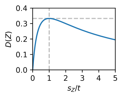
Figure 1: (Left) Plot of $\textstyle D(Z)=\big{|}\frac{t}{2t+s_{Z}}-\frac{3t}{5t+s_{Z}}\big{|}+\big{|}\frac{t}{2t+s_{Z}}-\frac{2t}{5t+s_{Z}}\big{|}$ from the proof of Theorem 1. (Right) Plot of $D(Z)=\big{|}\frac{2t}{2t+s_{Z}}-\frac{t/2}{t/2+s_{Z}}\big{|}$ from the proof of Theorem 2. Both functions are re-parameterized in terms of the ratio $s_{Z}/t$ by dividing through by $t$ and achieve local optima at $s_{Z}/t=1$ (i.e. $s_{Z}=t$); this can be verified analytically.

4.2 Disagreement

Using a similar strategy, we can construct an MNL instance whose disagreement is maximized rather than minimized at a particular target value (Theorem 2). The reduction requires an even simpler MNL setup.

Theorem 2.

In the MNL model, Disagreement is NP-hard, even with just one item in $C$ and two individuals that have identical utilities on items in $\overline{C}$.

Proof.

By reduction from Subset Sum (Karp, 1972). Let $S$ be a set of positive integers with target $t$. Let $A=\{a,b\}$, $C=\{x\}$, $\overline{C}=S$, with utilities: $u_{a}(x)=\log 2t$, $u_{b}(x)=\log t/2$, and $u_{a}(z)=u_{b}(z)=\log z$ for all $z\in\overline{C}$. Letting $s_{Z}=\sum_{z\in Z}z$, including $Z\subseteq\overline{C}$ makes the disagreement

$$D(Z)=\left|\frac{2t}{2t+s_{Z}}-\frac{t/2}{t/2+s_{Z}}\right|.$$

For $s_{Z}\geq 0$, $D(Z)$ is maximized at $s_{Z}=t$ (Fig. 1, right). Thus, if we could efficiently maximize $D(Z)$, then we could efficiently solve Subset Sum. ∎

By Lemma 1, we again have the following corollary.

Corollary 2.

Disagreement is NP-hard in the CDM, NL, and EBA models.

4.3 Promotion

In choice models with no context effects, Promotion has a constant-time solution: under IIA, the presence of alternatives has no effect on an individual’s relative preference for items in $C$. However, Promotion is more interesting with context effects, and we show that it is NP-hard for CDM, NL, and EBA. In Section 4.4, we will show that restrictions of these models make Promotion tractable but keep Agreement and Disagreement hard.

Theorem 3.

In the CDM model, Promotion is NP-hard, even with just one individual and three items in $C$.

Proof.

By reduction from Subset Sum. Let set $S$ with target $t$ be an instance of Subset Sum. Let $A=\{a\}$, $C=\{x^{*},w,y\}$, $\overline{C}=S$. Using tuples interpreted entry-wise for brevity, suppose that we have the following utilities:

$$u_{a}(\langle x^{*},w,y\rangle\mid C) =\langle 1,t,-t\rangle$$

$$u_{a}(z) =-\infty \forall z\in\overline{C}$$

$$p_{a}(z,\langle x^{*},w,y\rangle) =\langle z,0,2z\rangle \forall z\in\overline{C}.$$

We wish to promote $x^{*}$. Let $s_{Z}=\sum_{z\in Z}z$. When we include the alternatives in $Z$, $x^{*}$ is the item in $C$ most likely to be chosen if and only if $1+s_{Z}>t$ and $1+s_{Z}>-t+2s_{Z}$. Since $s_{Z}$ and $t$ are integers, this is only possible if $s_{Z}=t$. Thus, if we could efficiently promote $x^{*}$, then we could efficiently solve Subset Sum. ∎

We use the same Goldilocks strategy in our proofs for the NL and EBA models: by carefully defining utilities, we create choice instances where the optimal promotion solution is to pick just the right quantity of alternatives to increase preference for one item without overshooting. However, the NL model has a novel challenge compared to the CDM. With CDM, alternatives can increase the choice probability of an item in $C$, but in the NL, new alternatives only lower choice probabilities.

Theorem 4.

In the NL model, Promotion is NP-hard, even with just two individuals and two items in $C$.

Proof.

By reduction from Subset Sum. Let $S=\{z_{1},\dots,z_{n}\},t$ be an instance of Subset Sum. Let $A=\{a,b\}$, $C=\{x^{*},y\}$, $\overline{C}=S$, and $0<\varepsilon<1$. The nest structures and utilities are shown in Fig. 2.

for tree= l sep=3em, s sep=1em, , [$a$’s root [$y$, edge label=node[midway, left] 0] [$r$, edge label=node[midway, right] $\log 2$ [$x^{*}$, edge label=node[midway, left] $\log(t+\varepsilon)\;$] [$z_{1}$, edge label=node[midway, below right] $\log z_{1}$] […, no edge] [$z_{n}$, edge label=node[midway, above right] $\log z_{n}$] ] ]   for tree= l sep=3em, s sep=1em, , [$b$’s root [$x^{*}$, edge label=node[midway, left] 0] [$r$, edge label=node[midway, right] $\log 2$ [$y$, edge label=node[midway, left] $\log(t-\varepsilon)\;$] [$z_{1}$, edge label=node[midway, below right] $\log z_{1}$] […, no edge] [$z_{n}$, edge label=node[midway, above right] $\log z_{n}$] ] ]

Figure 2: NL trees used in the proof of Theorem 4. The left tree is for individual $a$ and the right tree for individual $b$.

We wish to promote $x^{*}$. With just the choice set $C$, $a$ prefers $x^{*}$ to $y$, but $b$ does not. To make $b$ prefer $x^{*}$ to $y$, we need to cannibalize $y$ by adding $z_{i}$ items. However, this simultaneously cannibalizes $x^{*}$ in $a$’s tree, so we need to be careful not to introduce too much additional utility. To ensure $a$ prefers $x^{*}$, we need to pick $Z$ such that

$$\Pr(a\leftarrow y\mid C\cup Z) <\Pr(a\leftarrow y\mid C\cup Z)$$

$$\iff\frac{1}{1+e^{\log 2}} <\frac{e^{\log 2}}{1+e^{\log 2}}\cdot\frac{e^{\log(t+\varepsilon)}}{e^{\log(t+\varepsilon)}+\sum_{z\in Z}e^{\log z}}$$

$$\iff\frac{1}{3} <\frac{2}{3}\cdot\frac{t+\varepsilon}{t+\varepsilon+\sum_{z\in Z}z}$$

$$\iff\sum_{z\in Z}z <t+\varepsilon.$$

To ensure $b$ prefers $x^{*}$, we need

$$\Pr(b\leftarrow x^{*}\mid C\cup Z) >\Pr(b\leftarrow y\mid C\cup Z)$$

$$\iff\frac{1}{1+e^{\log 2}} >\frac{e^{\log 2}}{1+e^{\log 2}}\cdot\frac{e^{\log(t-\varepsilon)}}{e^{\log(t-\varepsilon)}+\sum_{z\in Z}e^{\log z}}$$

$$\iff\frac{1}{3} >\frac{2}{3}\cdot\frac{t-\varepsilon}{t-\varepsilon+\sum_{z\in Z}z}$$

$$\iff\sum_{z\in Z}z >t-\varepsilon.$$

Since the $z$ are all integers, we must then have $\sum_{z\in Z}z=t$. If we could efficiently promote $x^{*}$, we could efficiently find such a $Z$. ∎

This nested logit construction relies on the two individuals having different nesting structures: notice that $x^{*}$ and $y$ are swapped in the two trees. We will see in Section 4.4 that this is a necessary condition for the hardness of Promotion under the nested logit model.

Finally, we have the following hardness result for EBA.

Theorem 5.

In the EBA model, Promotion is NP-hard, even with just two individuals and two items in $C$.

Proof.

By reduction from Subset Sum. Let $S,t$ be an instance of Subset Sum. Let $A=\{a,b\}$, $C=\{x^{*},y\}$, $\overline{C}=S$, and $s=\sum_{z\in S}z$. Make aspects $\chi_{z},\psi_{z},\gamma_{z}$ for each $z\in S$ as well as two more aspects $\chi,\psi$. The items have aspects as follows:

$$x^{*\prime} =\{\chi\}\cup\{\chi_{z}\mid z\in S\}$$

$$y^{\prime} =\{\psi\}\cup\{\psi_{z}\mid z\in S\}$$

$$z^{\prime} =\{\chi_{z},\psi_{z},\gamma_{z}\} \forall z\in S$$

The individuals have the following utilities on aspects, where $0<\varepsilon<1$:

$$\begin{aligned} u_{a}(\chi)&=0\\ u_{a}(\chi_{z})&=z\\ u_{a}(\psi)&=s-t/2-\varepsilon\\ u_{a}(\psi_{z})&=0\\ u_{a}(\gamma_{z})&=s-z\end{aligned}\;\begin{aligned} u_{b}(\chi)&=s-t/2+\varepsilon\\ u_{b}(\chi_{z})&=0\\ u_{b}(\psi)&=0\\ u_{b}(\psi_{z})&=z\\ u_{b}(\gamma_{z})&=s-z\end{aligned}\;\begin{aligned} &\\ &\forall z\in S\\ &\\ &\forall z\in S\\ &\forall z\in S\end{aligned}$$

We want to promote $x^{*}$. Notice that $x^{*}$ and $y$ have disjoint aspects. Thus the choice probabilities from $C$ are proportional to the sum of the item’s aspects:

$$\Pr(a\leftarrow x^{*}\mid C) \propto s\phantom{\frac{t}{2}}$$

$$\Pr(a\leftarrow y\mid C) \propto s-\frac{t}{2}-\varepsilon$$

$$\Pr(b\leftarrow x^{*}\mid C) \propto s-\frac{t}{2}+\varepsilon$$

$$\Pr(b\leftarrow y\mid C) \propto s.\phantom{\frac{t}{2}}$$

To promote $x^{*}$, we need to make $b$ prefer $x^{*}$ to $y$. Adding a $z$ item cannibalizes from $a$’s preference for $x^{*}$ and $b$’s preference for $y$. As in the NL proof, we want to add just enough $z$ items to make $b$ prefer $x^{*}$ to $y$ without making $a$ prefer $y$ to $x^{*}$.

First, notice that the $\gamma_{z}$ aspects have no effect on the individuals’ relative preference for $x^{*}$ and $y$. If we introduce the alternative $z$, then if $a$ picks the aspect $\chi_{z}$, $y$ will be eliminated. The remaining aspects of $x^{*}$, namely $x^{*\prime}\setminus\{\chi_{z}\}$, have combined utility $s-z$, as does $\gamma_{z}$. Therefore $a$ will be equallly likely to pick $x^{*}$ and $z$. Symmetric reasoning shows that if $b$ chooses aspect $\psi_{z}$, then $b$ will end up picking $y$ with probability 1/2. This means that when we include alternatives $Z\subseteq\overline{C}$, each aspect $\chi_{z},\psi_{z}$ for $z\in Z$ effectively contributes $z/2$ to $a$’s utility for $x^{*}$ and $b$’s utility for $y$ rather than the full $z$. The optimal solution is therefore a set $Z$ of alternatives whose sum is $t$, since that will cause $a$ to have effective utility $s-t/2$ on $x^{*}$, which exceeds its utility $s-t/2-\varepsilon$ on $y$. Meanwhile, $b$’s effective utility on $y$ will also be $s-t/2$, which is smaller than its utility $s-t/2+\varepsilon$ on $x^{*}$. If we include less alternative weight, $b$ will prefer $y$. If we include more, $a$ will prefer $y$. Therefore if we could efficiently find the optimal set of alternatives to promote $x^{*}$, we could efficiently find a subset of $S$ with sum $t$. ∎

4.4 Restricted models that make promotion easier

We now show that, in some sense, Promotion is a fundamentally easier problem than Agreement or Disagreement. Specifically, there are simple restrictions on CDM, NL, and EBA that make Promotion tractable but leave Agreement and Disagreement NP-hard. Importantly, these restrictions still allow for choice set effects. In Section 4.5, we also prove a strong restriction on the MNL model where Agreement and Disagreement are tractable, but we could not find meaningful restrictions for similar results on the other models.

2-item CDM with equal context effects.  The proof of Theorem 3 shows that Promotion is hard with only a single individual and three items in $C$. However, if $C$ only has two items and context effects are the same (i.e., $p_{a}(z,\cdot)$ is the same for all $z\in\overline{C}$), then Promotion is tractable. The optimal solution is to include all alternatives that increase utility for $x^{*}$ more than the other item, as doing so makes strict progress on promoting $x^{*}$. If individuals have different context effects or if there are more than two items, then there can be conflicts between which items should be included (see Section A.1 for a proof that 2-item CDM with unequal context effects makes Promotion NP-hard). Although this restriction makes Promotion tractable, it leaves Agreement and Disagreement NP-hard: the proofs of Theorems 1 and 2 can be interpreted as 2-item and 1-item CDMs with equal (zero) context effects.

Same-tree NL.  If we require that all individuals share the same NL tree structure, but still allow different utilities, then promotion becomes tractable. For each $z\in\overline{C}$, we can determine whether it reduces the relative choice probability of $x^{*}$ based on its position in the tree: adding $z$ decreases the relative choice probability of $x^{*}$ if and only if $z$ is a sibling of any ancestor of $x^{*}$ (including $x^{*}$) or if it causes such a sibling to be added to $T_{a}(C)$. Thus, the solution to Promotion is to include all $z$ not in those positions, which is a polynomial-time check. This restriction leaves Agreement and Disagreement NP-hard via Theorems 1 and 2 as we can still encode any MNL model in a same-tree NL using the tree in which all items are children of the root.

Disjoint-aspect EBA.  The following condition on aspects makes promoting $x^{*}$ tractable: for all $z\in\overline{C}$, either $z^{\prime}\cap x^{*\prime}=\emptyset$ or $z^{\prime}\cap y^{\prime}=\emptyset$ for all $y\in C$, $y\neq x^{*}$. That is, alternatives either share no aspects with $x^{*}$ or share no aspects with other items in $C$. This prevents alternatives from cannibalizing from both $x^{*}$ and its competitors. To promote $x^{*}$, we include all alternatives that share aspects with competitors of $x^{*}$ but not $x^{*}$ itself, which strictly promotes $x^{*}$. This condition is slightly weaker than requiring all items to have disjoint aspects, which reduces to MNL. However, this condition is again not sufficient to make Agreement and Disagreement tractable, since any MNL model can be encoded in a disjoint-aspect EBA instance.

4.5 Strong restriction on MNL that makes Agreement and Disagreement tractable

As we saw in the proofs of Theorems 1 and 2, Agreement and Disagreement are hard in the MNL model even when individuals have identical utilities on alternatives. This is possible because the individuals have different sums of utilities on $C$; one unit of utility on an alternative has a weaker effect for individuals with higher utility sums on $C$. To address the issue of identifiability, we assume each individual’s utility sum over $\mathcal{U}$ is zero in this section. This allows us to meaningfully compare the sum of utilities of two different individuals.

Definition 1.

If an individual $a$ has $\sum_{x\in\mathcal{U}}u_{a}(x)=0$, then the stubbornness of $a$ is $\sigma_{a}=\sum_{x\in C}e^{u(x)}.$

We call this quantity “stubbornness” since it quantifies how reluctant an individual is to change its probabilities on $C$ given a unit of utility on an alternative.

Proposition 1.

In an MNL model where all individuals are equally stubborn and have identical utilities on alternatives, the solution to Agreement is $\overline{C}$.

Proof.

Assume utilities are in standard form, with $\sum_{x\in\mathcal{U}}u_{a}(x)=0$. Let $\sigma=\sum_{x\in C}e^{u(x)}$ be each individual’s stubborness and let $Z$ be a set of alternatives. Suppose all individuals have the same utility $u(z)$ for each alternative $z$. The disagreement between two individuals about a single item $x$ in $C$ is then:

$$\Big{|}\frac{e^{u_{a}(x)}}{\sigma+\sum_{z\in Z}e^{u(z)}}-\frac{e^{u_{b}(x)}}{\sigma+\sum_{z\in Z}e^{u(z)}}\Big{|}=\frac{|e^{u_{a}(x)}-e^{u_{b}(x)}|}{\sigma+\sum_{z\in Z}e^{u(z)}}.$$

Notice that this strictly decreases if $\sum_{z\in Z}e^{u(z)}$ increases, so we minimize $D$ by including all of the alternatives. ∎

The same reasoning also allows us to trivially solve Disagreement in this restricted MNL model.

Corollary 3.

The solution to Disagreement in an equal alternative utilities, equal stubbornness MNL model is $\emptyset$.

While this MNL restriction is too strong to be of practical value, it is interesting from a theoretical perspective as it indicates where the hardness of the problem arises.

5 Approximation algorithms

Algorithm 1 $\varepsilon$-additive approximation for Agreement in the MNL model.

1   Input: $n$ individuals $A$, $k$ items $C$, $m$ alternatives $\overline{C}$, utilities $u_{a}(\cdot)>0$ for each $a\in A$. For brevity:

2   $e_{ax}\leftarrow e^{u_{a}(x)}$,  $s_{a}\leftarrow\sum_{z\in\overline{C}}e_{az}$,  $\delta\leftarrow\varepsilon/(2km\binom{n}{2})$

3   $L_{0}\leftarrow$ empty $n$-dimensional array whose $a$th dimension has size $1+\lfloor\log_{1+\delta}s_{a}\rfloor$ (each cell can store a set $Z\subseteq\overline{C}$ and its $n$ exp-utility sums for each individual)

4   Initialize $L_{0}[0,\dots,0]\leftarrow(\emptyset,0,\dots,0)$ ($n$ zeros)

5   for $i=1$ to $m$ do

6       $z\leftarrow\overline{C}[i-1]$,   $L_{i}\leftarrow L_{i-1}$

7       for each cell of $L_{i-1}$ containing $(Z,t_{1},\dots,t_{n})$ do

8            $h\leftarrow$ $n$-tuple w/ entries $\lfloor\log_{1+\delta}(t_{j}+e_{a_{j}z})\rfloor$, $\forall j$

9            if $L_{i}[h]$ is empty then

10                $L_{i}[h]\leftarrow(Z\cup\{z\},t_{1}+e_{a_{1}z},\dots,t_{n}+e_{a_{n}z})$

11   $Z_{m}\leftarrow$ collection of all sets $Z$ in cells of $L_{m}$

12   return  $\arg\min_{Z\in Z_{m}}D(Z)$ (see Eq. 4)

Thus far, we have seen that several interesting group decision-making problems are NP-hard across standard discrete choice models. Here, we provide a positive result: we can compute arbitrarily good approximate solutions to many instances of these problems in polynomial time. We focus our analysis on Algorithm 1, which is an $\varepsilon$-additive approximation algorithm to Agreement under MNL, with runtime polynomial in $k$, $m$, and $\frac{1}{\varepsilon}$, but exponential in $n$ (recall that $k=|C|$, $m=|\overline{C}|$, and $n=|A|$). In contrast, brute force (testing every set of alternatives) is exponential in $m$ and polynomial in $k$ and $n$. Agreement is NP-hard even with $n=2$ (Theorem 1), so our algorithm provides a substantial efficiency improvement. We discuss how to extend this algorithm to other objectives and other choice models later in the section. Finally, we present a faster but less flexible mixed-integer programming approach for MNL Agreement and Disagreement that performs very well in practice.

Algorithm 1 is based on an FPTAS for Subset Sum (Cormen et al., 2001, Sec. 35.5), and the first parts of our analysis follow some of the same steps. The core idea of our algorithm is that a set of items can be characterized by its exp-utility sums for each individual and that there are only polynomially many combinations of exp-utility sums that differ by more than a multiplicative factor $1+\delta$. We can therefore compute all sets of alternatives with meaningfully different impacts and pick the best one. For the purpose of the algorithm, we assume all utilities are positive (otherwise we may access a negative index); utilities can always be shifted by a constant to satisfy this requirement.

Figure 3: Example of the structure $L_{i}$ used in Algorithm 1 for $n=3$ individuals and $\overline{C}=\{\bigstar,\blacksquare\}$. Here, Alice has high utility for $\bigstar$ and low utility for $\blacksquare$, Bob has medium utility for $\bigstar$ and low utility for $\blacksquare$, and Carla has low utility for $\bigstar$ and high utility for $\blacksquare$. The exp-utility sums stored in cells are omitted.

We now provide an intuitive description of Algorithm 1. The array $L_{i}$ has one dimension for each individual in $A$ (we use a hash table in practice since $L_{i}$ is typically sparse). The cells along a particular dimension discretize the exp-utility sums that the individual corresponding to that dimension could have for a particular set of alternatives (Figure 3). In particular, if individual $j$ has total exp-utility $t_{j}=\sum_{y\in Z}e^{u_{j}(y)}$ for a set $Z$, then we store $Z$ at index $\lfloor\log_{1+\delta}t_{j}\rfloor$ along dimension $j$.

As the algorithm progresses, we place possible sets of alternatives $Z$ in the cells of $L_{i}$ according to their exp-utility sums $t_{1},\dots,t_{n}$ for each individual (we store $t_{1},\dots,t_{n}$ in the cell along with $Z$). We add one element at a time from $\overline{C}$ to the sets already in $L_{i}$ ($L_{0}$ starts with only the empty set). If two sets have very similar exp-utility sums, they may map to the same cell, in which case only one of them is stored. If the discretization of the array is coarse enough (that is, with large enough $\delta$), many sets of alternatives will map to the same cells, reducing the number of sets we consider and saving computational work. On the other hand, if the discretization is fine enough ($\delta$ is sufficiently small), then the best set we are left with at the end of the algorithm cannot induce a disagreement value too different from the optimal set. We now formalize this reasoning, starting with the following technical lemma that shows items mapping to same cell have similar exp-utility sums.

Lemma 2.

Let $\overline{C}_{i}$ be the first $i$ elements processed by the outer for loop of Algorithm 1. At the end of the algorithm, for all $Z\subseteq\overline{C}_{i}$ with exp-utility sums $t_{a}$, there exists some $Z^{\prime}\in L_{i}$ with exp-utility sums $t_{a}^{\prime}$ such that $\frac{t_{a}}{(1+\delta)^{i}}<t_{a}^{\prime}<t_{a}(1+\delta)^{i}$, for all $a\in A$ (with $\delta$ as defined in Algorithm 1, Line 2).

Proof.

If a set $Z$ has total exp-utility $t_{a}$ to individual $a$, then it is placed in $L$ at position $\lfloor\log_{1+\delta}t_{a}\rfloor$ in dimension $a$. So, if two sets $Z$, $Z^{\prime}$ with exp-utility totals $t_{a},t_{a}^{\prime}$ for individual $a$ are mapped to the same cell of $L$, then for all $a\in A$, $\lfloor\log_{1+\delta}t_{a}\rfloor=\lfloor\log_{1+\delta}t_{a}^{\prime}\rfloor$. We can therefore bound $t_{a}^{\prime}$:

$$\log_{1+\delta}t_{a}-1<\log_{1+\delta}t_{a}^{\prime}<\log_{1+\delta}t_{a}+1.$$

Exponentiating both sides with base $1+\delta$ and simplifying yields

$$\frac{t_{a}}{1+\delta}<t_{a}^{\prime}<t_{a}(1+\delta).$$ (5)

With this fact in hand, we proceed by induction on $i$. When $i=0$, $\overline{C}_{i}$ is empty and the lemma holds. Now suppose that $i>0$ and that the lemma holds for $i-1$. Every set in $\overline{C}_{i}$ was made by adding (a) zero elements or (b) one element to a set in $\overline{C}_{i-1}$. We consider these two cases separately.

(a) For any set $Z\subseteq\overline{C}_{i}$ that is also contained in $\overline{C}_{i-1}$, we know by the inductive hypothesis that some element in $L_{i-1}$ satisfied the inequality. Since we never overwrite cells, the lemma also holds for $Z$ after iteration $i$.

(b) Now consider sets $Z^{\prime}\subseteq\overline{C}_{i}$ that were formed by adding the new element $z$ to a set $Z\subseteq\overline{C}_{i-1}$. In the inner for loop, we at some point encountered the cell containing the set $Y\in L_{i-1}$ satisfying the lemma for set $Z$ by the inductive hypothesis. Let $y_{a}$ be the exp-utility totals for $Y$ and $t_{a}$ for $Z$. Notice that the exp-utility totals of $Z^{\prime}$ are exactly $t_{a}+e_{az}$. Starting with the inductive hypothesis, we see that the exp-utility totals of $Y\cup\{z\}$ satisfy

$$\frac{t_{a}+e_{az}}{(1+\delta)^{i-1}}<y_{a}+e_{az}<(t_{a}+e_{az})(1+\delta)^{i-1}.$$

When we go to place $Y\cup\{z\}$ in a cell, it might be unoccupied, in which case we place it in $L_{i}$ and the lemma holds for $Z^{\prime}$. If it is occupied by some other set, then by applying Eq. 5 we find that the lemma also holds for $Z^{\prime}$. ∎

With this lemma in hand, we can prove our main constructive result.

Theorem 6.

Algorithm 1 is an $\varepsilon$-additive approximation for Agreement in the MNL model.

Proof.

Let $\beta=\varepsilon/(k\binom{n}{2})$ for brevity. Following our choice of $\delta$ and using Lemma 2, at the end of the algorithm, the optimal set $Z^{*}\subseteq\overline{C}$ (with exp-utility sums $t_{a}^{*}$) has some representative $Z^{\prime}$ in $L_{m}$ such that

$$\frac{t_{a}^{*}}{(1+\beta/(2m))^{m}}<t_{a}^{\prime}<t_{a}^{*}\left(1+\beta/(2m)\right)^{m},\;\forall a\in A.$$

Since $e^{x}\geq(1+x/m)^{m}$, we have $t_{a}^{*}/e^{\frac{\beta}{2}}<t_{a}^{\prime}<t_{a}^{*}e^{\frac{\beta}{2}}$, and since $e^{x}\leq 1+x+x^{2}$ when $x<1$,

$$\frac{t_{a}^{*}}{1+\beta/2+\beta^{2}/4}<t_{a}^{\prime}<t_{a}^{*}(1+\beta/2+\beta^{2}/4).$$

Finally, $\frac{t_{a}^{*}}{1+\beta}<t_{a}^{\prime}<t_{a}^{*}(1+\beta)$ because $0<\beta<1$.

Now we show that $D(Z^{*})$ and $D(Z^{\prime})$ differ by at most $\varepsilon$. To do so, we first bound the difference between $\Pr(a\leftarrow x\mid C\cup Z^{*})$ and $\Pr(a\leftarrow x\mid C\cup Z^{\prime})$ by $\beta$. Let $c_{a}=\sum_{x\in C}e_{ax}$ be the total exp-utility of $a$ on $C$. By the above reasoning,

$$\frac{e_{ax}}{c_{a}+t_{a}^{*}(1+\beta)}<\frac{e_{ax}}{c_{a}+t_{a}^{\prime}}<\frac{e_{ax}}{c_{a}+\frac{t_{a}^{*}}{1+\beta}},$$

where the middle term is equal to $\Pr(a\leftarrow x\mid C\cup Z^{\prime})$. From the lower bound, the difference between $\Pr(a\leftarrow x\mid C\cup Z^{*})$ and $\Pr(a\leftarrow x\mid C\cup Z^{\prime})$ could be as large as

$$\frac{e_{ax}}{c_{a}+t_{a}^{*}}-\frac{e_{ax}}{c_{a}+t_{a}^{*}(1+\beta)}$$

$$=\frac{e_{ax}t_{a}^{*}\beta}{(c_{a}+t_{a}^{*})(c_{a}+t_{a}^{*}(1+\beta))}<\frac{e_{ax}t_{a}^{*}\beta}{2c_{a}t_{a}^{*}}\leq\frac{\beta}{2}.$$

From the upper bound, the difference between $\Pr(a\leftarrow x\mid C\cup Z^{*})$ and $\Pr(a\leftarrow x\mid C\cup Z^{\prime})$ could be as large as

$$\frac{e_{ax}}{c_{a}+\frac{t_{a}^{*}}{1+\beta}}-\frac{e_{ax}}{c_{a}+t_{a}^{*}}=\frac{e_{ax}t_{a}(1-\frac{1}{1+\beta})}{(c_{a}+\frac{t_{a}^{*}}{1+\beta})(c_{a}+t_{a}^{*})}$$

$$=\frac{e_{ax}t_{a}^{*}\beta}{(c_{a}(1+\beta)+t_{a}^{*})(c_{a}+t_{a}^{*})}<\frac{e_{ax}t_{a}^{*}\beta}{2c_{a}t_{a}^{*}}\leq\frac{\beta}{2}.$$

Thus, $\Pr(a\leftarrow x\mid C\cup Z^{*})$ and $\Pr(a\leftarrow x\mid C\cup Z^{\prime})$ differ by at most $\frac{\beta}{2}$. Using the same argument for an individual $b$, the disagreement between $a$ and $b$ about $x$ can only increase by $\beta$ with the set $Z$ compared to the optimal set $Z^{*}$. Since there are $\binom{n}{2}$ pairs of individuals and $k$ items in $C$, the total error of the algorithm is bounded by $k\binom{n}{2}\beta=\varepsilon$. ∎

We now show that the runtime of Algorithm 1 is $O((m+kn^{2})(1+\lfloor\log_{1+\delta}s\rfloor)^{n})$, where $s=\max_{a}s_{a}$ is the maximum exp-utility sum for any individual. Moreover, for any fixed $n$, this runtime is bounded by a polynomial in $k,m$, and $\frac{1}{\varepsilon}$.

To see this, first note that the size of $L_{i}$ is bounded above by $(1+\lfloor\log_{1+\delta}s\rfloor)^{n}$. For each $z\in\overline{C}$, we perform constant-time operations on each entry of $L_{i}$, for a total of $O(m(1+\lfloor\log_{1+\delta}s\rfloor)^{n})$ time. Then we compute $D(Z)$ for each cell of $L_{m}$, which takes $O(kn^{2})$ time per cell. The total runtime is therefore $O((m+kn^{2})(1+\lfloor\log_{1+\delta}s\rfloor)^{n})$, as claimed. Finally, $(1+\lfloor\log_{1+\delta}s\rfloor)^{n}$ is bounded by a polynomial in $m,k$, and $\frac{1}{\varepsilon}$ for any fixed $n$:

$$(1+\lfloor\log_{1+\delta}s\rfloor)^{n} \leq\Big{(}1+\frac{\ln s}{\ln 1+\delta}\Big{)}^{n}$$

$$\leq\Big{(}1+(1+\delta)\frac{\ln s}{\delta}\Big{)}^{n} \ln(1+x)\geq\frac{x}{1+x} x>-1$$ (since for )

$$=\Big{(}1+\frac{\ln s}{\delta}+\ln s\Big{)}^{n}$$

$$=\Big{(}1+\frac{2km\binom{n}{2}\ln s}{\varepsilon}+\ln s\Big{)}^{n}.$$

Agreement is NP-hard even when individuals have equal utilities on alternatives. In this case, we only need to compute exp-utility sums for a single individual, which brings the runtime down to $O((m+kn^{2})\log_{1+\delta}s)$.

Extensions to other objectives and models.  Algorithm 1 can be easily extended to any objective function that is efficiently computable from utilities. For instance, Algorithm 1 can be adapted for Disagreement by replacing the $\arg\min$ with an $\arg\max$ on Line 12.

Algorithm 1 can also be adapted for CDM and NL. The analysis is similar and details are in Appendix B, although the running times and guarantees are different. With CDM, the exponent in the runtime increases to $nk$ for Agreement and Disagreement, and the $\varepsilon$-additive approximation is guaranteed only if items in $\overline{C}$ exert zero pulls on each other. However, even for the general CDM, our experiments will show that the adapted algorithm remains a useful heuristic. When we adapt Algorithm 1 for NL, we retain the full approximation guarantee but the exponent in the runtime increases and has a dependence on the tree size.

Promotion is not interesting under MNL and also has a discrete rather than continuous objective, i.e., the number of people with favorite item $x^{*}$ in $C$. For models with context effects, we can define a meaningful notion of approximation.

Definition 2.

An item $y\in C\cup Z$ is an $\varepsilon$-favorite item of individual $a$ if $\Pr(a\leftarrow y\mid C\cup Z)+\varepsilon\geq\Pr(a\leftarrow x\mid C\cup Z)$ for all $x\in C$. A solution $\varepsilon$-approximates Promotion if the number of people for whom $x^{*}$ is an $\varepsilon$-favorite item is at least the value of the optimal Promotion solution.

Using this, we can adapt Algorithm 1 for Promotion under CDM and NL. Again, for CDM, the approximation has guarantees in certain parameter regimes and the NL has full approximation guarantees. Since we do not have compute $D(Z)$, the runtimes loses the $kn^{2}$ term compared to the Agreement and Disagreement versions (Section B.3).

Finally, EBA has considerably different structure than the other models. We leave algorithms for EBA to future work.

5.1 Fast exact methods for MNL

We provide another approach for solving Agreement and Disagreement in the MNL model, based on transforming the objective functions into mixed-integer bilinear programs (MIBLPs). MIBLPs can be solved for moderate problem sizes with high-performance branch-and-bound solvers (we use Gurobi’s implementation). In practice, this approach is faster than Algorithm 1 (for finding optimal solutions—Algorithm 1 will always be faster with sufficiently large $\varepsilon$) and can optimize over larger sets $\overline{C}$. However, this approach does not easily extend to CDM, NL, or Promotion and does not have a polynomial-time runtime guarantee.

5.1.1 MIBLP formulation for Agreement

Let $x_{i}$ be a decision variable indicating whether we add in the $i$th item in $\overline{C}$. Let $e_{ya}=e^{u_{a}(y)}$ and $e_{Ca}=\sum_{y\in C}e_{ya}$. We can write Agreement as the following 0-1 optimization problem.

$$\underset{\displaystyle x}{\mathrm{min}}\quad\sum_{a,b\in A}\sum_{y\in C}\left|\frac{e_{ya}}{e_{Ca}+\sum_{i\in\overline{C}}x_{i}e_{ia}}-\frac{e_{yb}}{e_{Cb}+\sum_{i\in\overline{C}}x_{i}e_{ib}}\right|$$

$$x_{i}\in\{0,1\}$$

We can rewrite this with no absolute values by introducing new variables $\delta_{yab}$ that represent the absolute disagreement about item $y$ between individuals $a$ and $b$. We then use the standard trick for minimizing an absolute value in linear programs:

To get rid of the fractions, we introduce the new variables $z_{a}=\frac{1}{e_{Ca}+\sum_{i}x_{i}e_{ia}}$ for each individual $a$ and add corresponding constraints enforcing the definition of $z_{a}$:

5.1.2 MIBLP formulation for Disagreement

A similar technique works for Disagreement, but maximizing an absolute value is slightly trickier than minimizing. In addition to the variables $\delta_{yab}$ that we used before, we also add new binary variables $g_{yab}$ indicating whether each difference in choice probabilities is positive or negative. With these new variables (and following the same steps as above), Disagreement can be written as the following MIBLP:

6 Numerical experiments

We apply our methods to three datasets (Table 1). The SFWork dataset (Koppelman & Bhat, 2006) comes from a survey of San Francisco residents on available (choice set) and selected (choice) transportation options to get to work. We split the respondents into two segments ($\lvert A\rvert=2$) according to whether or not they live in the “core residential district of San Fransisco or Berkeley.” The Allstate dataset (Kaggle, 2014) consists of insurance policies (items) characterized by anonymous categorical features A–G with 2 to 4 values each. Each customer views a set of policies (the choice set) before purchasing one. We reduce the number of items to 24 by considering only features A, B, and C. To model different types of individuals, we split the data into homeowners and non-homeowners (again, $\lvert A\rvert=2$). The Yoochoose dataset (Ben-Shimon et al., 2015) contains online shopping data of clicks and purchases of categorized items in user browsing sessions. Choice sets are unique categories browsed in a session and the choice is the category of the purchased product (categories appearing fewer than 20 times were omitted). We split the choice data into two sub-populations by thresholding on the purchase timestamps.

For inferring maximum-likelihood models from data, we use PyTorch’s Adam optimizer (Kingma & Ba, 2015; Paszke et al., 2019) with learning rate $0.05$, weight decay $0.00025$, batch size 128, and the amsgrad flag (Reddi et al., 2018). We use the low-rank (rank-2) CDM (Seshadri et al., 2019) that expresses pulls as the inner product of item embeddings. Our code and data are available at https://github.com/tomlinsonk/choice-set-opt.

Table 1: Dataset statistics: item, observation, and unique choice set counts; and percent of observations in sub-population splits.

Dataset	# items	# obs.	# sets	split %
SFWork	6	5029	12	16/84
Allstate	24	97009	2697	45/55
Yoochoose	41	90493	1567	47/53

Table 2: Sum of error over all 2-item choice sets $C$ compared to optimal (brute force) on SFWork. Algorithm 1 is optimal.

Model	Problem	Greedy	Algorithm 1
MNL	Agreement	$0.03$	$0.00$
	Disagreement	$0.00$	$0.00$
rank-2 CDM	Agreement	$0.14$	$0.00$
	Disagreement	$0.13$	$0.00$
NL	Agreement	$0.00$	$0.00$
	Disagreement	$0.00$	$0.00$

For SFWork under the MNL, CDM, and NL models, we considered all 2-item choice sets $C$ (using all other items for $\overline{C}$) for Agreement and Disagreement (for the NL model, we used the best-performing tree from Koppelman & Bhat (2006)). We compare Algorithm 1 ($\varepsilon=0.01$) to a greedy approach (henceforth, “Greedy”) that builds $Z$ by repeatedly selecting the item from $\overline{C}$ that, when added to $Z$, most improves the objective, if such an item exists. This dataset was small enough to compare against the optimal, brute-force solution (Table 2). In all cases, Algorithm 1 finds the optimal solution, while Greedy is often suboptimal. However, for this value of $\varepsilon$, we find that Algorithm 1 searches the entire space and actually computes the brute force solution (we get the number of sets analyzed by Algorithm 1 from $|L_{m}|$ for a given $\varepsilon$ and compare it to $2^{\lvert\overline{C}\rvert}$). Even though we have an asymptotic polynomial runtime guarantee, for small enough datasets, we might not see computational savings. Running with larger $\varepsilon$ yielded similar results, even for $\varepsilon>2$, when our bounds are vacuous.

The results still highlight two important points. First, even on small datasets, Greedy can be sub-optimal. For example, for Agreement under CDM with $C=\{\text{drive alone},\text{transit}\}$, Algorithm 1 found the optimal $Z=\{\text{bike, walk}\}$, inferring that both sub-populations agree on both driving less and taking transit less. However, Greedy just introduced a carpool option, which has a lower effect on discouraging driving alone or taking transit, resulting in lower agreement between city and suburban residents.

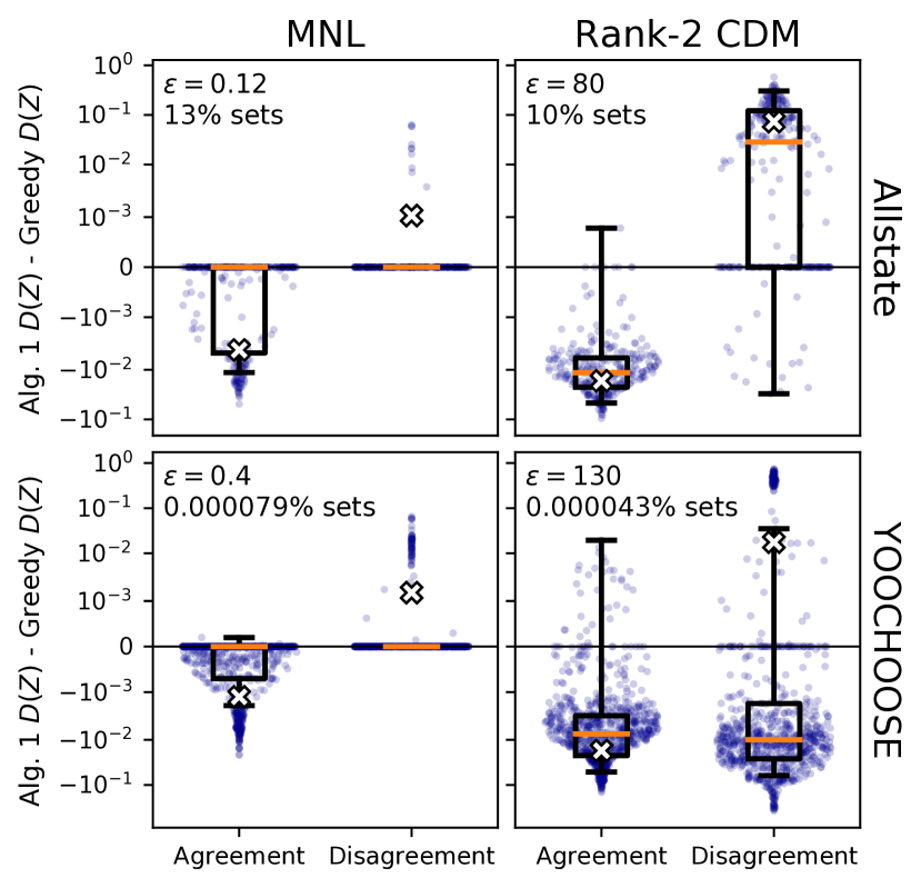
Figure 4: Algorithm 1 vs. Greedy performance box plots when applied to all 2-item choice sets in Allstate and Yoochoose under MNL and CDM (subplots also show $\varepsilon$ and the percent of subsets of $\overline{C}$ computed by Algorithm 1, written X% sets). Each point is the difference in $D(Z)$ when Algorithm 1 and Greedy are run on a particular choice set. Horizontal spread shows approximate density and the Xs mark means. A negative (resp. positive) $y$-value for Agreement (resp. Disagreement) indicates that Algorithm 1 outperformed Greedy. Algorithm 1 performs better in all cases except for Disagreement under CDM on Yoochoose. Even in this exception, though, our approach finds a few very good solutions and Algorithm 1 has better mean performance.

Second, our theoretical bounds can be more pessimistic than what happens in practice. Thus, we can consider larger values of $\varepsilon$ to reduce the search space; Algorithm 1 remains a principled heuristic, and we can measure how much of the search space Algorithm 1 considers. This is the approach we take for the Allstate and Yoochoose data, where we find that Algorithm 1 far outperforms its theoretical worst-case bound. We again considered all 2-item choice sets $C$ and tested our method under MNL and CDM, setting $\varepsilon$ so that the experiment took about 30 minutes to run for Allstate and 2 hours for Yoochoose (of that time, Greedy takes 5 seconds to run; the rest is taken up by Algorithm 1). Algorithm 1 consistently outperforms Greedy (Fig. 4), even with $\varepsilon>2$ for CDM. Moreover, Algorithm 1 only computes a small fraction of possible sets of alternatives, especially for Yoochoose. Algorithm 1 does not perform as well with the rank-2 CDM as it does with MNL, which is to be expected as we only have approximation guarantees for CDM under particular parameter regimes (in which these data do not lie). The worse performance on CDM is due to the context effects that items from $\overline{C}$ exert on each other. Greedy does fairly well for Disagreement under CDM with Yoochoose, but even in this case, Algorithm 1 performs significantly better in enough instances for the mean (but not median) performance to be better than Greedy. We repeated the experiment with 500 choice sets of size up to 5 sampled from data with similar results (Section C.3). We also ran the MIBLP approach for MNL, which performed as well as Algorithm 1 and was about $12$x faster on Yoochoose and $240$x faster on Allstate with the $\varepsilon$ values we used for Algorithm 1 (Section C.2).

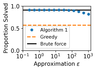
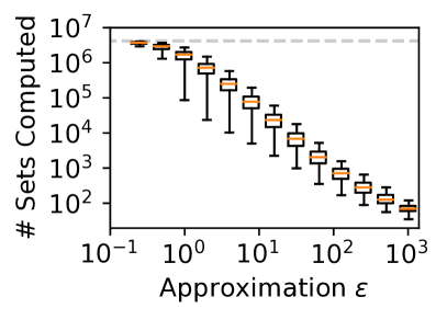
Figure 5: Promotion results on Allstate 2-item choice sets. (Left) Success rate comparison; Algorithm 1 has near-optimal performance (about $9\%$ of instances have no Promotion solution). (Right) Number of subsets of $\overline{C}$ computed by Algorithm 1 (dashed gray line at $2^{22}=2^{m}$ for brute force computation).

Promotion.  We applied the CDM Promotion version of Algorithm 1 to Allstate, since this dataset is small enough to compute brute-force solutions. For each 2-item choice set $C$, we attempted to promote the less-popular item of the pair using brute-force, Greedy, and Algorithm 1. Algorithm 1 performed optimally up to $\varepsilon=32$, above which it failed in only 2–26 of 252 feasible instances (Fig. 5, left). (Here, successful promotion means that the item becomes the true favorite among $C$.) On the other hand, Greedy failed in $37\%$ of the feasible instances. As in the previous experiment, our algorithm’s performance in practice far exceeds the worst-case bounds. The number of sets tested by Algorithm 1 falls dramatically as $\varepsilon$ increases (Fig. 5, right). With more items (or a smaller range of utilities), the value of $\varepsilon$ required to achieve the same speedup over brute force would be smaller (as with Yoochoose). In tandem, these results show that we get near-optimal Promotion performance with far fewer computations than brute force.

7 Discussion

Our decisions are influenced by the alternatives that are available, the choice set. In collective decision-making, altering the choice set can encourage agreement or create new conflict. We formulated this as an algorithmic question: how can we optimize the choice set for some objective?

We showed that choice set optimization is NP-hard for natural objectives under standard choice models; however, we also found that model restrictions makes promoting a choice easier than encouraging a group to agree or disagree. We developed approximation algorithms for these hard problems that are effective in practice, although there remains a gap between theoretical approximation bounds and performance on real-world data. Future work could address choice set optimization in interactive group decisions, where group members can communicate their preferences to each other or must collaborate to reach a unified decision. Lastly, Appendix D discusses the ethical considerations of this work.

Appendix A Hardness proofs

A.1 CDM Promotion is hard with $|A|=2,|C|=2$

In the main text, we show CDM Promotion is NP-hard when $|A|=1,|C|=3$ (Theorem 3). Here, we provide an additonal proof for the case when $|A|=2,|C|=2$. These are the smallest hard instances of the problem ($|A|=1,|C|=2$ is easy to solve: introduce alternatives that increase utility for $x^{*}$ for than its competitor).

Theorem 7.

In the CDM model, Promotion is NP-hard, even with just two individuals and two items in $C$.

Proof.

By reduction from Subset Sum. Let $S,t$ be an instance of Subset Sum. Let $A=\{a,b\}$, $C=\{x,y\}$, $\overline{C}=S$. Using tuples interpreted entrywise, construct a CDM with the following parameters.

$$u_{a}(\langle x^{*},y\rangle) =\langle t+\varepsilon,0\rangle$$

$$u_{b}(\langle x^{*},y\rangle) =\langle\varepsilon,t\rangle$$

$$u_{a}(z) =u_{b}(z)=-\infty \forall z\in\overline{C}$$

$$p_{a}(z,\langle x^{*},y\rangle) =\langle 0,z\rangle \forall z\in\overline{C}$$

$$p_{b}(z,\langle x^{*},y\rangle) =\langle z,0\rangle \forall z\in\overline{C}$$

To promote $x^{*}$, we need to add more than $t-\varepsilon$ to $b$’s utility for $x^{*}$, but add less than $t+\varepsilon$ to $a$’s utility for $x^{*}$. Since all pulls are integral, the only solution is a set $Z$ whose sum of pulls is $t$. If we could efficiently find such a set, then we could efficiently find the Subset Sum solution. ∎

Appendix B Approximation algorithm extensions

B.1 Adapting Algorithm 1 for CDM with guarantees for special cases

We can adapt Algorithm 1 for the CDM model, but we only maintain the approximation error bounds under special cases of the structure of the “pulls”. Still, we can use this algorithm as a principled heuristic and it tends to work well in practice, as we saw in Fig. 4.

As a first step, we use the alternative parametrization of the model used by Seshadri et al. (2019, Eq. (1)), which has fewer parameters. In this description of the model, utilities and context effects are merged into a single utility-adjusted pull $q_{a}(z,x)=p_{a}(z,x)-u_{a}(x)$, with the special case $q_{a}(x,x)=0$. We then have

$$\Pr(a\leftarrow x\mid C)=\frac{\exp({\sum_{w\in C}q_{a}(w,x)})}{\sum_{y\in C}\exp({\sum_{z\in C}q_{a}(z,y)})}.$$ (6)

Refer to Seshadri et al. (2019, Appendix C.1) for details of the equivalence between this formulation and the one we use in the main text.

Matching the notation of the proof of Theorem 6, we use the shorthand $e_{ax}=\exp({\sum_{w\in C}q_{a}(w,x)})$.

To adapt Algorithm 1 to the CDM, we expand $L_{i}$ to have $nk$ dimensions for each individual-item pair, increasing the runtime to $O((m+kn^{2})(1+\lfloor\log_{1+\delta}s\rfloor)^{nk})$. This is only practical if $nk$ is small, but as we have seen, Agreement, Disagreement, and Promotion are all NP-hard even with $n=2$ and $k=2$ or $3$. Each individual-item dimension stores $e_{ax}$, the total exp-utility of that item to that individual given that we have included some set of alternatives. When we include an additional item from $\overline{C}$, we place the new sets in $L_{i}$ with updated $e_{ax}$ values.

This only preserves the $\varepsilon$-additive approximation if alternatives (items in $\overline{C}$) have zero context effects on each other; however, they may still have context effects on items in $C$. Formally, we need $q_{a}(z,z^{\prime})=0$ for all $z,z^{\prime}\in\overline{C}$ and $a\in A$. Although this is a serious restriction, it leaves Agreement, Disagreement, and Promotion NP-hard, as the CDM we used in our proofs had this form (see also Section B.3 for how to apply Algorithm 1 to Promotion). If this version of the algorithm is applied to a general CDM, it may experience higher error. Nonetheless, our real-data experiments show it to be a good heuristic.

For the following analysis, we assume a CDM with zero context effects between items in $\overline{C}$. We need to verify that if every item’s exp-utility is approximated to within factor $(1+\beta)^{\pm 1}$, then the total disagreement of a set is approximated to within $\varepsilon$ as we had in the MNL case. The approximation error guarantee increases to $4\varepsilon$ in the restricted CDM version—to recover the $\varepsilon$-additive approximation, we can make $\delta$ smaller by a factor of 4 (that is, we could pick $\delta=\varepsilon/(8km\binom{n}{2})$; we instead keep the old $\delta$ for simplicity in the following analysis).

Recall that $Z^{\prime}$ is the representative in $L_{m}$ of the optimal set of alternatives $Z^{*}$. For compactness, we define $T_{a}$ to be the denominator of Eq. 6, with $T_{a}^{\prime}$ and $T_{a}^{*}$ referring to those denominators under the choice sets $C\cup Z^{\prime}$ and $C\cup Z^{*}$, respectively. This is where we require zero context effects between alternatives: if alternatives interact, then storing every $e_{ax}$ in the table (from which we can compute $T_{a}$) is not enough to determine updated choice probabilities when we add a new alternative.

The difference in the analysis begins when we bound $\Pr(a\leftarrow x\mid C\cup Z^{\prime})$ on both sides using the fact that each exp-utility sum is approximated within a $1+\beta$ factor (so the probability denomiators $T_{a}$ are also approximated within this factor):

$$\frac{\frac{e_{ax}^{*}}{1+\beta}}{T_{a}^{*}(1+\beta)} =\frac{1}{(1+\beta)^{2}}\frac{e_{ax}^{*}}{T_{a}^{*}}$$

$$<\frac{e_{ax}^{\prime}}{T_{a}^{\prime}}=\Pr(a\leftarrow x\mid C\cup Z^{\prime})$$

$$<\frac{e_{ax}^{*}(1+\beta)}{\frac{T_{a}^{*}}{1+\beta}}=(1+\beta)^{2}\frac{e_{ax}^{*}}{T_{a}^{*}}.$$

Based on the lower bound, the difference between $\Pr(a\leftarrow x\mid C\cup Z^{*})$ and $\Pr(a\leftarrow x\mid C\cup Z^{\prime})$ could be as large as

$$\frac{e_{ax}^{*}}{T_{a}^{*}}-\frac{1}{(1+\beta)^{2}}\frac{e_{ax}^{*}}{T_{a}^{*}} \leq 1-\frac{1}{(1+\beta)^{2}}.$$

Now considering the upper bound, the difference between $\Pr(a\leftarrow x\mid C\cup Z^{*})$ and $\Pr(a\leftarrow x\mid C\cup Z^{\prime})$ could be as large as

$$(1+\beta)^{2}\frac{e_{ax}^{*}}{T_{a}^{*}}-\frac{e_{ax}^{*}}{T_{a}^{*}} \leq(1+\beta)^{2}-1.$$

Therefore, $|\Pr(a\leftarrow x\mid C\cup Z^{\prime})-\Pr(b\leftarrow x\mid C\cup Z^{\prime})|$ can only exceed $|\Pr(a\leftarrow x\mid C\cup Z^{*})-\Pr(b\leftarrow x\mid C\cup Z^{*})|$ by at most $1-\frac{1}{(1+\beta)^{2}}+(1+\beta)^{2}-1=(1+\beta)^{2}-\frac{1}{(1+\beta)^{2}}$. This is at most $4\beta$:

$$4\beta-(1+\beta)^{2}+\frac{1}{(1+\beta)^{2}} =\frac{\beta^{2}(2-\beta^{2})}{(1+\beta)^{2}}$$

$$>0. 0<\beta<\sqrt{2}$$ (for )

So $D(Z^{\prime})$ and $D(Z^{*})$ are within $4\beta\binom{n}{2}k=4\varepsilon$.

B.2 Adapting Algorithm 1 for NL with full guarantees

We can also adapt Algorithm 1 for the NL model, and unlike the CDM, the $\varepsilon$-additive approximation holds in all parameter regimes. Recall that the NL tree has two types of leaves: choice set items and alternative items. Let $P_{a}$ be the set of internal nodes of individual $a$’s tree that have at least one alternative item as a child and let $p=\max_{a\in A}|P_{a}|$. If we know the total exp-utility that alternatives contribute as children of each $v\in P_{a}$, then we can compute $a$’s choice probabilites over items in $C$ in polynomial time.

With this in mind, we modify Algorithm 1 by having dimensions in $L$ for each individual for each of their nodes in $P_{a}$. This results in $\leq np$ dimensions. The algorithm then keeps track of the exp-utility sums from alternatives under each node in $P_{a}$ for each individual. The exponent in the runtime increases to (at most) $np$, but this remains tractable for some hard instances, such as those in our hardness proofs. In some cases, we can dramatically improve the runtime of the algorithm: if the subtree under an internal node contains only alternatives as leaves in an individuals’s tree, then we only need one dimension $L$ for that individual’s entire subtree, and it has only two cells: one for sets that contain at least one alternative in that subtree, and one for sets that do not. The only factor that affects the choice probabilities of items in $C$ is whether that subtree is “active” and its root can be chosen.

We now show how the error from exp-utility sums of alternatives propagates to choice probabilities. In the NL model, $\Pr(a\leftarrow x\mid C)$ is the product of probabilities that $a$ chooses each ancestor of $x$ as $a$ descends down its tree. Let $v_{1},\dots,v_{\ell}$ be the nodes in $a$’s tree along the path from the root to $x$. For compactness, we use $\Pr(x,Z)$ instead of $\Pr(a\leftarrow x\mid C\cup Z)$ in the following analysis.

Pick $\delta\leq([\varepsilon/(2k\binom{n}{2})+1]^{1/\ell}-1)/m$ and recall that $\beta=2m\delta$. We can use the same analysis as in the proof of Theorem 6 to find that for any set $Z^{*}\subseteq\overline{C}$, there exists some $Z^{\prime}\in L$ such that

$$\Pr(x,Z^{*}) =\Pr(v_{1},Z^{*})\cdot\dots\cdot\Pr(v_{x},Z^{*})$$

$$<\Big{(}\Pr(v_{1},Z^{\prime})+\frac{\beta}{2}\Big{)}\cdot\dots\cdot\Big{(}\Pr(v_{x},Z^{\prime})+\frac{\beta}{2}\Big{)}$$

$$\leq\Pr(x,Z^{\prime})+\Big{(}1+\frac{\beta}{2}\Big{)}^{\ell}-1$$

$$\leq\Pr(x,Z^{\prime})+\frac{\varepsilon}{2k\binom{n}{2}}.$$

Now for the lower bound, pick $\delta\leq(1-[1-\varepsilon/(2k\binom{n}{2})]^{1/\ell})/m$. Again from the proof of Theorem 6:

$$\Pr(x,Z^{*}) =\Pr(v_{1},Z^{*})\cdot\dots\cdot\Pr(v_{x},Z^{*})$$

$$>\Big{(}\Pr(v_{1},Z^{\prime})-\frac{\beta}{2}\Big{)}\cdot\dots\cdot\Big{(}\Pr(v_{x},Z^{\prime})-\frac{\beta}{2}\Big{)}$$

$$\geq\Pr(x,Z^{\prime})+\Big{(}1-\frac{\beta}{2}\Big{)}^{\ell}-1$$

$$\geq\Pr(x,Z^{\prime})-\frac{\varepsilon}{2k\binom{n}{2}}.$$

Let $h$ be the maximum height of any indivdual’s NL tree (so $\ell\leq h$). Then, by picking $\delta=\min\{[\varepsilon/(2k\binom{n}{2})+1]^{1/h}-1,1-[1-\varepsilon/(2k\binom{n}{2})]^{1/h}\}/m$, we find that $\Pr(a\leftarrow x\mid C\cup Z^{*})$ and $\Pr(a\leftarrow x\mid C\cup Z^{\prime})$ differ by less than $\varepsilon/(k\binom{n}{2})$ for all $x\in C$ and $a\in A$, meaning that the total disagreement between $a$ and $b$ cannot differ by more than $\varepsilon$ as before.

Unfortunately, this means we need to make $\delta$ exponentially (in $h$) smaller in the NL model. Put another way, our error bound gets exponentially worse as $h$ increases if we keep $\delta$ constant. However, we have seen that there are NP-hard families of NL instances in which $h$ is a small constant (e.g., $h=2$ in our hardness proof), so once again this algorithm is an exponential improvement over brute force. Moreover, the error bound here is often far from tight, since we use the very loose bounds $\Pr(v_{i},Z^{\prime})\leq 1$ in the analysis. This means the algorithm will tend to outperform the worst-case guarantee by a significant margin.

B.3 Adapting Algorithm 1 for Promotion

B.3.1 CDM Promotion with special case guarantees

Algorithm 1 can be applied to Promotion in the (restricted) CDM model with only a small modification to the CDM version described in Section B.1: at the end of the algorithm, we return the set that results in the maximum number of individuals having $x^{*}$ as an $\varepsilon$-favorite item. Additionally, we choose $\delta=\varepsilon/(10m)$ (we don’t need the factors $\binom{n}{2}$ or $k$ since we aren’t optimizing $D(Z)$).

Following the analysis in Section B.1 (with $\beta=2m\delta=\varepsilon/5$), we find that $\Pr(a\leftarrow x\mid C\cup Z^{*})$ and $\Pr(a\leftarrow x\mid C\cup Z^{\prime})$ differ by at most $\max\{1-\frac{1}{(1+\varepsilon/5)^{2}},(1+\varepsilon/5)^{2}-1\}$ for all $x$. On the interval $[0,1]$, this is bounded by $\varepsilon/2$. Thus, if $x^{*}$ is the favorite item for $a$ given the optimal choice set $C\cup Z^{*}$, then it must be an $\varepsilon$-favorite of individual $a$ given $C\cup Z^{\prime}$ (as always, $Z^{\prime}$ is the representative of $Z^{*}$ in $L_{m}$). This is because when we go from $C\cup Z^{*}$ to $C\cup Z^{\prime}$, the choice probability of $x^{*}$ can shrink by at most $\varepsilon/2$ and the choice probability for any other item can grow by at most $\varepsilon/2$. Thus, including $Z^{\prime}$ makes at least as many individuals have $x^{*}$ as an $\varepsilon$-favorite item as including $Z^{*}$ makes have $x^{*}$ as a favorite item.

This is exactly what it means for Algorithm 1 to $\varepsilon$-approximate Promotion in the CDM (when items in $\overline{C}$ do not exert context effects on each other). Moreover, not having to compute $D(Z)$ makes the runtime of Algorithm 1 $O(m(1+\lfloor\log_{1+\delta}s\rfloor)^{nk})$ when applied to Promotion in the CDM. In the general CDM, this algorithm is only a heuristic.

B.3.2 NL Promotion with full guarantees

A very similar idea allows us to apply the NL version of Algorithm 1 from Section B.2 to Promotion and retain an approximation guarantee. As before, use the NL version and return the set that results in the maximum number of individuals having $x^{*}$ as an $\varepsilon$-favorite item. However, we instead use $\delta=\min\{(\varepsilon/4+1)^{1/h}-1,1-(1-\varepsilon/4)^{1/h}\}/m$, which by the analysis in Section B.2 results in $\Pr(a\leftarrow x\mid C\cup Z^{*})$ and $\Pr(a\leftarrow x\mid C\cup Z^{\prime})$ differing by at most $\varepsilon/2$. As in the CDM case, this guarantees that if $x^{*}$ is the favorite item for $a$ given the optimal choice set $C\cup Z^{*}$, then it must be an $\varepsilon$-favorite of $a$ given $C\cup Z^{\prime}$. Therefore this version of Algorithm 1 $\varepsilon$-approximates Promotion in the NL model with runtime $O(m(1+\lfloor\log_{1+\delta}s\rfloor)^{np})$.

Appendix C Additional experiment details

C.1 Simple example of poor performance for Greedy

As we saw in experimental data, Greedy can perform poorly even in small instances of Agreement. Below we provide an MNL instance with $n=m=k=2$ for which the error of the greedy solution is approximately 1. With only two individuals, $0\leq D(Z)\leq 2$, so an error of 1 is very large.

In the bad instance for greedy, $A=\{a,b\}$, $C=\{x,y\}$, $\overline{C}=\{p,q\}$, and the utilities are as follows.

$$\begin{aligned} u_{a}(x)&=8\\ u_{a}(y)&=2\\ u_{a}(p)&=10\\ u_{a}(q)&=0\end{aligned}\qquad\begin{aligned} u_{b}(x)&=8\\ u_{b}(y)&=8\\ u_{b}(p)&=0\\ u_{b}(q)&=15\end{aligned}$$

In this instance of Agreement, the greedy solution is $D(\emptyset)\approx 0.9951$ (including either $p$ or $q$ alone increases disagreement), while the optimal solution is $D(\{p,q\})\approx 0.0009$.

C.2 All-pairs agreement results for MIBLP

Figure 6 shows the comparison in performance between Algorithm 1 and the MIBLP approach for the all-pairs Agreement and Disagreement experiment. The methods perform nearly identically on both Allstate and Yoochoose. The MIBLP approach performs marginally better in some cases of Yoochoose Agreement. As noted in the paper, the MIBLP heuristic is considerably faster for the values of $\varepsilon$ we used ($12$x and $240$x on Yoochoose and Allstate, respectively; speed differences vary significantly depending on $\varepsilon$), but provides no a priori performance guarantee and cannot be applied to CDM or NL. Nonetheless, we can see that it performs very competitively and would be a good approach to use in practice for MNL Agreement and Disagreement.

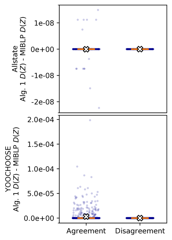
Figure 6: MIBLP vs. Algorithm 1 performance box plots when applied to all 2-item choice sets in Allstate and Yoochoose under MNL. Each point is the difference in $D(Z)$ when MIBLP and Algorithm 1 are run on a choice set, and Xs mark means.

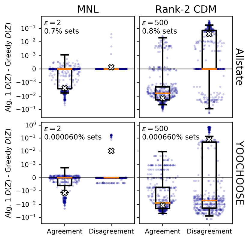
Figure 7: Results of the agreement experiment with 500 choice sets sampled uniformly from each dataset. Compare with Fig. 4 in the main text. Again, Algorithm 1 has better mean performance in all cases. The larger values of $\varepsilon$ result in slightly worse performance on the margins than in Fig. 4, but also fewer sets computed.

C.3 Choice sets sampled from data

We repeated the all-pairs agreement experiment with 500 choice sets of size up to 5 sampled uniformly from each dataset, allowing us to evaluate the performance of Algorithm 1 on realistic choice sets. We limited the size of sampled choice sets since the CDM version of Algorithm 1 scales poorly with $|C|$ (see Section B.1). For this version of the experiment, we fixed larger values of $\varepsilon$ (2 for MNL, 500 for CDM) to handle larger choice sets and to keep running time down. Again, Algorithm 1 has better mean performance in every case (Fig. 7), showing that it performs well on real choice sets.

Appendix D A note on ethical considerations

Influencing the preferences of decision-makers has the potential for malicious applications, so it is important to address the ethical context of this work.

Any problem with positive social applications (e.g., Agreement: encouraging consensus, Promotion: promoting environmentally-friendly transportation options, Disagreement: increasing diversity of opinions) has the potential to be used for ill. This should not prevent us from seeking methods to acheive these positive ends, but we should certainly be cognizant of the possibility of unintended applications. In a different vein, understanding when a group is susceptible to undesired interventions (or detecting such interventions) makes problems like Disagreement worth studying from an adversarial perspective. Along these lines, our hardness results are encouraging since optimal malicious interventions are difficult.

Finally, we note that all of the theoretical problems we study presuppose access to choice data from which preferences can be learned and the ability to influence choice sets. Any entity which has both of these (such as an online retailer, a government deciding transportation policy, etc.) already has significant power to influence choosers. If such an entity had malicious intent, then near-optimal Disagreement solutions would be the least of our concerns.

To summarize, these problems are worth studying because of (1) their purely theoretical value in furthering the field of discrete choice, (2) their potential for positive applications, (3) insight into the potential for harmful manipulation by an adversary, and (4) the minimal additional risk from undesired use of our methods.

References

- Amir et al. (2015) Amir, O., Grosz, B. J., Gajos, K. Z., Swenson, S. M., and Sanders, L. M. From care plans to care coordination: Opportunities for computer support of teamwork in complex healthcare. In Proceedings of the 33rd Annual ACM Conference on Human Factors in Computing Systems, pp. 1419–1428. ACM, 2015.
- Ammar et al. (2014) Ammar, A., Oh, S., Shah, D., and Voloch, L. F. What’s your choice?: learning the mixed multi-nomial. In ACM SIGMETRICS Performance Evaluation Review, pp. 565–566. ACM, 2014.
- Ben-Shimon et al. (2015) Ben-Shimon, D., Tsikinovsky, A., Friedmann, M., Shapira, B., Rokach, L., and Hoerle, J. RecSys challenge 2015 and the YOOCHOOSE dataset. In Proceedings of the 9th ACM Conference on Recommender Systems, pp. 357–358, 2015.
- Benson et al. (2016) Benson, A. R., Kumar, R., and Tomkins, A. On the relevance of irrelevant alternatives. In Proceedings of the 25th International Conference on World Wide Web, pp. 963–973. International World Wide Web Conferences Steering Committee, 2016.
- Benson et al. (2018) Benson, A. R., Kumar, R., and Tomkins, A. A discrete choice model for subset selection. In Proceedings of the Eleventh ACM International Conference on Web Search and Data Mining, pp. 37–45. ACM, 2018.
- Bower & Balzano (2020) Bower, A. and Balzano, L. Preference modeling with context-dependent salient features. In Proceedings of the 37th International Coference on International Conference on Machine Learning, 2020.
- Chen & Joachims (2016) Chen, S. and Joachims, T. Predicting matchups and preferences in context. In Proceedings of the 22nd ACM SIGKDD International Conference on Knowledge Discovery and Data Mining, pp. 775–784. ACM, 2016.
- Chen et al. (2018) Chen, X., Lijffijt, J., and De Bie, T. Quantifying and minimizing risk of conflict in social networks. In Proceedings of the 24th ACM SIGKDD International Conference on Knowledge Discovery & Data Mining, pp. 1197–1205. ACM, 2018.
- Chierichetti et al. (2018a) Chierichetti, F., Kumar, R., and Tomkins, A. Discrete choice, permutations, and reconstruction. In Proceedings of the Twenty-Ninth Annual ACM-SIAM Symposium on Discrete Algorithms, pp. 576–586. SIAM, 2018a.
- Chierichetti et al. (2018b) Chierichetti, F., Kumar, R., and Tomkins, A. Learning a mixture of two multinomial logits. In International Conference on Machine Learning, pp. 960–968, 2018b.
- Cormen et al. (2001) Cormen, T. H., Leiserson, C. E., Rivest, R. L., and Stein, C. Introduction to Algorithms. MIT Press, 2001.
- Davis et al. (2014) Davis, J. M., Gallego, G., and Topaloglu, H. Assortment optimization under variants of the nested logit model. Operations Research, 62(2):250–273, 2014.
- Easley & Kleinberg (2010) Easley, D. and Kleinberg, J. Networks, Crowds, and Markets. Cambridge University Press, 2010.
- Fader & McAlister (1990) Fader, P. S. and McAlister, L. An elimination by aspects model of consumer response to promotion calibrated on UPC scanner data. Journal of Marketing Research, 27(3):322–332, 1990.
- Gallego & Topaloglu (2014) Gallego, G. and Topaloglu, H. Constrained assortment optimization for the nested logit model. Management Science, 60(10):2583–2601, 2014.
- Garimella et al. (2017) Garimella, K., De Francisci Morales, G., Gionis, A., and Mathioudakis, M. Reducing controversy by connecting opposing views. In Proceedings of the Tenth ACM International Conference on Web Search and Data Mining, pp. 81–90. ACM, 2017.
- Graells-Garrido et al. (2014) Graells-Garrido, E., Lalmas, M., and Quercia, D. People of opposing views can share common interests. In Proceedings of the 23rd International Conference on World Wide Web, pp. 281–282. ACM, 2014.
- Hanley et al. (1998) Hanley, N., Wright, R. E., and Adamowicz, V. Using choice experiments to value the environment. Environmental and Resource Economics, 11(3-4):413–428, 1998.
- Hązła et al. (2017) Hązła, J., Jadbabaie, A., Mossel, E., and Rahimian, M. A. Bayesian decision making in groups is hard. arXiv:1705.04770, 2017.
- Hązła et al. (2019) Hązła, J., Jadbabaie, A., Mossel, E., and Rahimian, M. A. Reasoning in Bayesian opinion exchange networks is -hard. In Proceedings of the Thirty-Second Conference on Learning Theory, pp. 1614–1648, 2019.
- Huber et al. (1982) Huber, J., Payne, J. W., and Puto, C. Adding asymmetrically dominated alternatives: Violations of regularity and the similarity hypothesis. Journal of Consumer Research, 9(1):90–98, 1982.
- Ieong et al. (2012) Ieong, S., Mishra, N., and Sheffet, O. Predicting preference flips in commerce search. In Proceedings of the 29th International Coference on International Conference on Machine Learning, pp. 1795–1802. Omnipress, 2012.
- Kaggle (2014) Kaggle. Allstate purchase prediction challenge. https://www.kaggle.com/c/allstate-purchase-prediction-challenge, 2014.
- Kallus & Udell (2016) Kallus, N. and Udell, M. Revealed preference at scale: Learning personalized preferences from assortment choices. In Proceedings of the 2016 ACM Conference on Economics and Computation, pp. 821–837. ACM, 2016.
- Karp (1972) Karp, R. M. Reducibility among combinatorial problems. In Complexity of Computer Computations, pp. 85–103. Springer, 1972.
- Kingma & Ba (2015) Kingma, D. P. and Ba, J. Adam: A method for stochastic optimization. In International Conference on Learning Representations, 2015.
- Kleinberg et al. (2017) Kleinberg, J., Mullainathan, S., and Ugander, J. Comparison-based choices. In Proceedings of the 2017 ACM Conference on Economics and Computation, pp. 127–144. ACM, 2017.
- Koppelman & Bhat (2006) Koppelman, F. S. and Bhat, C. A self instructing course in mode choice modeling: Multinomial and nested logit models, 2006.
- Liao & Fu (2014) Liao, Q. V. and Fu, W.-T. Can you hear me now?: mitigating the echo chamber effect by source position indicators. In Proceedings of the 17th ACM Conference on Computer Supported Cooperative Work & Social Computing, pp. 184–196. ACM, 2014.
- Lu et al. (2012) Lu, L., Yuan, Y. C., and McLeod, P. L. Twenty-five years of hidden profiles in group decision making: A meta-analysis. Personality and Social Psychology Review, 16(1):54–75, 2012.
- Luce (1959) Luce, R. D. Individual Choice Behavior. Wiley, 1959.
- Makhijani & Ugander (2019) Makhijani, R. and Ugander, J. Parametric models for intransitivity in pairwise rankings. In The World Wide Web Conference, pp. 3056–3062. ACM, 2019.
- Matakos et al. (2017) Matakos, A., Terzi, E., and Tsaparas, P. Measuring and moderating opinion polarization in social networks. Data Mining and Knowledge Discovery, 31(5):1480–1505, 2017.
- Maystre & Grossglauser (2015) Maystre, L. and Grossglauser, M. Fast and accurate inference of Plackett–Luce models. In Advances in Neural Information Processing Systems, pp. 172–180, 2015.
- McFadden (1974) McFadden, D. Conditional logit analysis of qualitative choice behavior. In Zarembka, P. (ed.), Frontiers in Econometrics, pp. 105–142. Academic Press, 1974.
- McFadden (1978) McFadden, D. Modeling the choice of residential location. Transportation Research Record, 1978.
- McFadden & Train (2000) McFadden, D. and Train, K. Mixed MNL models for discrete response. Journal of Applied Econometrics, 15(5):447–470, 2000.
- Munson et al. (2013) Munson, S. A., Lee, S. Y., and Resnick, P. Encouraging reading of diverse political viewpoints with a browser widget. In Seventh International AAAI Conference on Weblogs and Social Media, 2013.
- Musco et al. (2018) Musco, C., Musco, C., and Tsourakakis, C. E. Minimizing polarization and disagreement in social networks. In Proceedings of the 2018 World Wide Web Conference, pp. 369–378. International World Wide Web Conferences Steering Committee, 2018.
- Oh & Shah (2014) Oh, S. and Shah, D. Learning mixed multinomial logit model from ordinal data. In Advances in Neural Information Processing Systems, pp. 595–603, 2014.
- Oh et al. (2015) Oh, S., Thekumparampil, K. K., and Xu, J. Collaboratively learning preferences from ordinal data. In Advances in Neural Information Processing Systems, pp. 1909–1917, 2015.
- Overgoor et al. (2019) Overgoor, J., Benson, A., and Ugander, J. Choosing to grow a graph: modeling network formation as discrete choice. In The World Wide Web Conference, pp. 1409–1420, 2019.
- Paszke et al. (2019) Paszke, A., Gross, S., Massa, F., Lerer, A., Bradbury, J., Chanan, G., Killeen, T., Lin, Z., Gimelshein, N., Antiga, L., et al. PyTorch: An imperative style, high-performance deep learning library. In Advances in Neural Information Processing Systems, pp. 8024–8035, 2019.
- Pfannschmidt et al. (2019) Pfannschmidt, K., Gupta, P., and Hüllermeier, E. Learning choice functions: Concepts and architectures. arXiv:1901.10860, 2019.
- Ragain & Ugander (2016) Ragain, S. and Ugander, J. Pairwise choice Markov chains. In Advances in Neural Information Processing Systems, pp. 3198–3206, 2016.
- Reddi et al. (2018) Reddi, S. J., Kale, S., and Kumar, S. On the convergence of Adam and beyond. In International Conference on Learning Representations, 2018.
- Rosenberg et al. (2020) Rosenberg, M., Perlroth, N., and Sanger, D. E. ‘Chaos is the point’: Russian hackers and trolls grow stealthier in 2020, 2020. URL https://www.nytimes.com/2020/01/10/us/politics/russia-hacking-disinformation-election.html.
- Rosenfeld et al. (2020) Rosenfeld, N., Oshiba, K., and Singer, Y. Predicting choice with set-dependent aggregation. In Proceedings of the 37th International Coference on International Conference on Machine Learning, 2020.
- Rusmevichientong et al. (2010) Rusmevichientong, P., Shen, Z.-J. M., and Shmoys, D. B. Dynamic assortment optimization with a multinomial logit choice model and capacity constraint. Operations Research, 58(6):1666–1680, 2010.
- Rusmevichientong et al. (2014) Rusmevichientong, P., Shmoys, D., Tong, C., and Topaloglu, H. Assortment optimization under the multinomial logit model with random choice parameters. Production and Operations Management, 23(11):2023–2039, 2014.
- Seshadri & Ugander (2019) Seshadri, A. and Ugander, J. Fundamental limits of testing the independence of irrelevant alternatives in discrete choice. In Proceedings of the 2019 ACM Conference on Economics and Computation, pp. 65–66, 2019.
- Seshadri et al. (2019) Seshadri, A., Peysakhovich, A., and Ugander, J. Discovering context effects from raw choice data. In International Conference on Machine Learning, pp. 5660–5669, 2019.
- Shafir et al. (1993) Shafir, E., Simonson, I., and Tversky, A. Reason-based choice. Cognition, 49(1-2):11–36, 1993.
- Simonson (1989) Simonson, I. Choice based on reasons: The case of attraction and compromise effects. Journal of Consumer Research, 16(2):158–174, 1989.
- Simonson & Tversky (1992) Simonson, I. and Tversky, A. Choice in context: Tradeoff contrast and extremeness aversion. Journal of Marketing Research, 29(3):281–295, 1992.
- Stasser & Titus (1985) Stasser, G. and Titus, W. Pooling of unshared information in group decision making: Biased information sampling during discussion. Journal of Personality and Social Psychology, 48(6):1467, 1985.
- Talluri & Van Ryzin (2004) Talluri, K. and Van Ryzin, G. Revenue management under a general discrete choice model of consumer behavior. Management Science, 50(1):15–33, 2004.
- Train (2009) Train, K. E. Discrete Choice Methods with Simulation. Cambridge University Press, 2009.
- Trueblood et al. (2013) Trueblood, J. S., Brown, S. D., Heathcote, A., and Busemeyer, J. R. Not just for consumers: Context effects are fundamental to decision making. Psychological Science, 24(6):901–908, 2013.
- Tversky (1972) Tversky, A. Elimination by aspects: A theory of choice. Psychological Review, 79(4):281, 1972.
- Tversky & Kahneman (1981) Tversky, A. and Kahneman, D. The framing of decisions and the psychology of choice. Science, 211(4481):453–458, 1981.
- Tversky & Simonson (1993) Tversky, A. and Simonson, I. Context-dependent preferences. Management Science, 39(10):1179–1189, 1993.
- Zhao & Xia (2019) Zhao, Z. and Xia, L. Learning mixtures of Plackett-Luce models from structured partial orders. In Advances in Neural Information Processing Systems, pp. 10143–10153, 2019.
- Zhao et al. (2016) Zhao, Z., Piech, P., and Xia, L. Learning mixtures of Plackett-Luce models. In International Conference on Machine Learning, pp. 2906–2914, 2016.