Superposition of FLRW Universes

Abstract

We show that (1) the Einstein field equations with a perfect fluid source admit a nonlinear superposition of two distinct homogenous Friedman-Lemaitre-Robertson-Walker (FLRW) metrics as a solution, (2) the superposed solution is an inhomogeneous geometry in general, (3) it reduces to a homogeneous one in the two asymptotes which are the early and the late stages of the universe as described by two different FLRW metrics, (4) the solution possesses a scale factor inversion symmetry and (5) the solution implies two kinds of topology changes: one during the time evolution of the superposed universe and the other occurring in the asymptotic region of space.

1 Introduction

An exact solution of the Einstein-perfect fluid system, representing an inhomogeneous cosmological model and admitting various interpretations, was recently rediscovered in [1] by the method of separation of variables. This solution is a subcase of the Kustaanheimo-Qvist class [2], and coincides with the other previously found solutions. See [2] and [3, 4] for the classification and interpretations of the previously found inhomogeneous cosmological solutions. One of the possible interpretations is that it is a generalization of the McVittie solution representing a black hole immersed in a FLRW universe [4, 7, 6, 8]. In this work we propose a different interpretation of our solution. The inhomogeneous cosmological model of [1] is a nonlinear superposition of generically two distinct FLRW universes with different spatial curvatures. Nonlinear superposition in general relativity has been studied in the context of Bäcklund transformations [9, 10, 11, 12] for spacetimes that possess two Killing vector fields. Here we give a novel example of a nonlinear superposition in general relativity. The FLRW phases show up in the early and late stages of the universe. Since each FLRW metric has a different spatial curvature, then in the early and late eras of the universe the spatial curvatures are different in general and a topology change is possible. The superposed model has a scale factor inversion symmetry akin to the scale factory duality symmetry observed earlier in string cosmology [13].

The layout of the paper is as follows. We first recapitulate the field equations of the inhomogeneous model in Section 2. In Section 3, we introduce a solution to the field equations possessing the scale factor inversion symmetry. In Section 4, we give two distinct interpretations of the obtained solution. We mainly discuss the second interpretation: superposition of two FLRW universes. In Section 5, we address two examples and discuss the features of our solution in the context of Big Bang and cyclic cosmological models [14, 15, 16]. Section 6 is devoted to our conclusions.

2 Matter-coupled field equations

We consider the spherically symmetric metric in isotropic coordinates

$$ds^{2}=-a^{2}(t,r)dt^{2}+c^{4}(t,r)\left(dr^{2}+r^{2}\,d\theta^{2}+r^{2}\,\sin^{2}\theta\,d\phi^{2}\right),$$ (2.1)

where $a(t,r)$ and $c(t,r)$ are generic differentiable functions of time $t$ and radial coordinate $r$. In [1], it was proven that the Einstein-perfect fluid field equations for $\dot{c}(t,r)\neq 0$ reduce to

$$2rcc^{\prime\prime}-6r{c^{\prime}}^{2}-2cc^{\prime}-h(r)=0,$$ (2.2)

$$a=2q(t)\,\frac{\dot{c}}{c},$$ (2.3)

where $h(r)$ is an arbitrary function of $r$ and $q(t)$ is an arbitrary function of $t$; the fluid velocity is given as $u_{\mu}=a\delta^{0}_{\mu}$. Here a dot and a prime denote differentiations with respect to $t$ and $r$, respectively. The energy density $\rho(t,r)$ and the pressure $p(t,r)$, respectively read as

$$8\pi\rho(t,r)=\frac{3}{q^{2}}-\frac{2}{rc^{6}}\left(6r{c^{\prime}}^{2}+6cc^{\prime}+h\right)-\Lambda,$$ (2.4)

$$8\pi p(t,r)=-\frac{3}{q^{2}}+\frac{1}{rq^{3}c{{}^{6}}\dot{c}}\,{\big{(}}2q^{3}\,(-r{c^{\prime}}^{2}\dot{c}+rcc^{\prime}\dot{c}^{\prime}+cc^{\prime}\dot{c}+c^{2}\dot{c}^{\prime})+rc^{7}\dot{q}{\big{)}}+\Lambda,$$ (2.5)

where $\Lambda$ is the cosmological constant. In [1], we discussed that if the metric functions $c(t,r)$ and $a(t,r)$ vanish on some surfaces then either $p$ or $\rho$ diverges, and hence the Ricci scalar $R=8\pi(\rho-3p)+4\Lambda$ diverges. These surfaces are defined as $\Sigma_{1}=\{(t,r)\in U|c(t,r)=0\}$ and $\Sigma_{2}=\{(t,r)\in U|a(t,r)=0\}$ where $U$ is a part of spacetime and $0<t<\infty,~{}r\geq 0$. In particular, the surface $\Sigma_{2}$ represents namely the cosmological singularities [17] or sudden cosmological singularities [18, 19, 20].

3 A solution to the field equations possessing the scale factor inversion symmetry

In [1], it was shown that

$$c(t,r)=\frac{\sqrt{R(t)}}{\sqrt{c_{0}+c_{1}r^{2}}}+\frac{\gamma}{\sqrt{R(t)}}\frac{1}{\sqrt{c_{2}+c_{3}r^{2}}},$$ (3.1)

is a solution to the ordinary nonlinear differential equation (2.2) with arbitrary constants $c_{0}$, $c_{1}$, $c_{2}$, $c_{3}$ and $\gamma$; and $R(t)$ is an at least twice differentiable function. For this solution, $h(r)$ is given by

$$h(r)=\frac{6\gamma(c_{0}\,c_{3}-c_{1}\,c_{2})^{2}r^{3}}{(c_{0}+c_{1}r^{2})^{\frac{5}{2}}(c_{2}+c_{3}r^{2})^{\frac{5}{2}}},$$ (3.2)

and furthermore choosing $q(t)=R(t)/\dot{R}(t)$, the lapse function reads as

$$a(t,r)=\frac{1-\frac{\gamma}{R(t)}\,\sqrt{\frac{c_{0}+c_{1}r^{2}}{c_{2}+c_{3}\,r^{2}}}}{1+\frac{\gamma}{R(t)}\,\sqrt{\frac{c_{0}+c_{1}r^{2}}{c_{2}+c_{3}r^{2}}}}.$$ (3.3)

Hence, the spacetime metric reads as

$$ds^{2}=-\left(\frac{1-\frac{\gamma}{R(t)}\,\sqrt{\frac{c_{0}+c_{1}r^{2}}{c_{2}+c_{3}\,r^{2}}}}{1+\frac{\gamma}{R(t)}\,\sqrt{\frac{c_{0}+c_{1}r^{2}}{c_{2}+c_{3}r^{2}}}}\right)^{2}dt^{2}$$

$$~{}~{}~{}~{}~{}~{}~{}~{}+\left(\frac{\sqrt{R(t)}}{\sqrt{c_{0}+c_{1}r^{2}}}+\frac{\gamma}{\sqrt{R(t)}}\frac{1}{\sqrt{c_{2}+c_{3}r^{2}}}\right)^{4}\left(dr^{2}+r^{2}\,d\theta^{2}+r^{2}\,\sin^{2}\theta\,d\phi^{2}\right).$$ (3.4)

Substituting (3.1) in (2.4) and (2.5), one can find the asymptotic form when $R(t)\to 0$ and keeping the leading orders, $\rho(t,r)$ and $p(t,r)$ become homogeneous and reduce to

$$8\pi\rho(t)\to 3\frac{{\dot{R}}^{2}}{R^{2}}+\frac{12c_{2}c_{3}R^{2}}{\gamma^{4}}-\Lambda,$$ (3.5)

$$8\pi p(t)\to 2\frac{{\ddot{R}}}{R}-5\frac{{\dot{R}}^{2}}{R^{2}}-\frac{4c_{2}c_{3}R^{2}}{\gamma^{4}}+\Lambda.$$ (3.6)

Similarly, $\rho(t,r)$ and $p(t,r)$ also become asymptotically homogeneous as $R(t)\to\infty$ and read as

$$8\pi\rho(t)\to 3\frac{{\dot{R}}^{2}}{R^{2}}+\frac{12c_{0}c_{1}}{R^{2}}-\Lambda,$$ (3.7)

$$8\pi p(t)\to-2\frac{{\ddot{R}}}{R}-\frac{{\dot{R}}^{2}}{R^{2}}-\frac{4c_{0}c_{1}}{R^{2}}+\Lambda.$$ (3.8)

Observe that the metric, i.e (3.1) and (3.3), is invariant under the scale factor inversion, as $R\to\gamma^{2}/R$, $c_{0}\leftrightarrow c_{2}$ and $c_{1}\leftrightarrow c_{3}$. This symmetry is akin to the scale factor duality symmetry in string cosmology [13]. This inversion symmetry can also be observed in the field equations: under this symmetry, the pair of equations (3.5) and (3.6) go to (3.7) and (3.8) and vice versa.

4 Interpretations of the solution

4.1 A generalized McVittie metric

Without losing any generality, one can choose the arbitrary constants $c_{0},c_{1},c_{2},c_{3}$ and $\gamma$ in such a way that the function $c(t,r)$ becomes

$$c(t,r)=\frac{\sqrt{R(t)}}{\sqrt{\mu+r^{2}}}+\frac{M}{2\sqrt{R(t)}}\frac{1}{\sqrt{1+kr^{2}}},$$ (4.1)

with three constants $M,k$ and $\mu$ representing the mass, spatial curvature of the background FLRW universe and the reduction parameter, respectively and $R(t)$ is the same function as in (3.1) up to a multiplicative constant. Letting $\mu=0$, the solution reduces to the uncharged Vaidya-Shah and the McVittie solution [5, 6], see also [3]. The McVittie solution can be interpreted as a black hole in a positively curved FLRW universe [7, 8]. Next we shall give another interpretation of this metric.

4.2 Superposition of two FLRW universes

One can arrange the constants $c_{0},c_{1},c_{2}$ and $c_{3}$ in (3.1) so that $c(t,r)$ takes the form

$$c(t,r)=\frac{\sqrt{R(t)}}{\sqrt{1+k_{1}r^{2}}}+\frac{\gamma}{\sqrt{R(t)}}\frac{1}{\sqrt{1+k_{2}r^{2}}},$$ (4.2)

where $k_{1}$, $k_{2}$ and $\gamma$ are arbitrary constants and and $R(t)$ is the same function as in (3.1) up to a multiplicative constant.

To show that the two FLRW metrics are nonlinearly superposed, we need to use the FLRW metric in the isotropic coordinates which reads

$$ds^{2}=-dt^{2}+\frac{R^{2}(t)}{(1+kr^{2})^{2}}\left(dr^{2}+r^{2}\,d\Omega^{2}\right),$$ (4.3)

where $R(t)$ is the scale factor and $k$ is 1/4 of the curvature constant of 3-space (lets call it $k_{*}$); and after making the coordinate $r$ unitless, $k_{*}$ can take the values $\pm 1$ and $0$. To discuss that our new solution represents the superposition of two FLRW universes, we consider the following two different FLRW universes in the isotropic coordinates $(t,r,\theta,\phi)$.

${\bf FLRW_{1}}$:

The metric for this case is given by

$$ds^{2}=-dt^{2}+c_{1}^{4}(t,r)\left(dr^{2}+r^{2}\,d\Omega^{2}\right),$$ (4.4)

where

$$c_{1}(t,r)=\frac{\sqrt{R(t)}}{\sqrt{1+k_{1}r^{2}}}.$$ (4.5)

This metric represents a FLRW universe with the scale factor $R(t)$ and the spatial curvature $k_{*}=4k_{1}$. The homogeneous matter density and pressure profiles for this case read as

$$8\pi\rho_{1}(t) = 3\frac{\dot{R}^{2}}{R^{2}}+3\frac{4k_{1}}{R^{2}}-\Lambda,$$ (4.6)

$$8\pi p_{1}(t) = -2\frac{\ddot{R}}{R}-\frac{\dot{R}^{2}}{R^{2}}-\frac{4k_{1}}{R^{2}}+\Lambda.$$ (4.7)

${\bf FLRW_{2}}$:

The metric for this case is given by

$$ds^{2}=-dt^{2}+c_{2}^{4}(t,r)\left(dr^{2}+r^{2}\,d\Omega^{2}\right),$$ (4.8)

where

$$c_{2}(t,r)=\frac{1}{\sqrt{R(t)}}\frac{1}{\sqrt{1+k_{2}r^{2}}}.$$ (4.9)

Then it represents a FLRW metric with the scale factor $R^{-1}(t)$ and the spatial curvature $k_{*}=4k_{2}$. Here, the matter density and pressure profiles are

$$8\pi\rho_{2}(t) = 3\frac{\dot{R}^{2}}{R^{2}}+12k_{2}R^{2}-\Lambda,$$ (4.10)

$$8\pi p_{2}(t) = 2\frac{\ddot{R}}{R}-5\frac{\dot{R}^{2}}{R^{2}}-4k_{2}R^{2}+\Lambda.$$ (4.11)

Now, regarding the above two cases, we have the following theorem indicating the second novel interpretation of the general solution (3.1) which we mainly discuss below.

Theorem: The linear superposition of $c_{1}(t,r)$ and $c_{2}(t,r)$, i.e. $c(t,r)=c_{1}(t,r)+\gamma c_{2}(t,r)$, with $c_{1}(t,r)$ and $c_{2}(t,r)$ given in (4.5) and (4.9) solves the Einstein field equations (2.2), (2.3), (2.4) and (2.5). Here, $\gamma$ is an arbitrary constant. Then, this represents a nonlinear superposition of two particular solutions (4.2) for which each part is generically a distinct FLRW universe with different spatial curvatures $k_{1}$ and $k_{2}$. If $k_{1}=k_{2}=k$, this general solution reduces to a single FLRW solution with the spatial curvature $k_{*}=4k$.

The model has a Big Bang singularity if $R\to 0$ as $t\to 0$ without further assumption on the energy density and pressure, this is the only constraint on the function $R$. Hence, each choice of $R$ generates a different cosmological model. For instance, assuming the scale factor to be $R(t)=R_{0}\left(e^{\lambda t}-1\right)^{n}$ where $R_{0}$, $\lambda$ and $n$ are positive constants, then from (3.5) and (3.6), one finds $\rho(t)\to\infty$ and $p(t)\to-\infty$ as $t\to 0$, respectively. In the limit $t\to\infty$, $R(t)\to\infty$ and from (3.7) and (3.8), one finds $\rho(t)\to 3n^{2}\lambda^{2}-\Lambda$ and $p(t)\to-3n^{2}\lambda^{2}+\Lambda$, respectively, which corresponds to a (anti)de Sitter space. In this case, the universe starts from a Big Bang and evolves to a pure (anti)de Sitter phase at late times.

Three consequences of the above theorem are as follows: $(i)$ the exact solution unifies two different homogeneous FLRW solutions in a single superposed solution which generally is inhomogeneous, $(ii)$ regarding (3.5)-(3.8), and (4.6), (4.7), (4.10) and (4.11), the universe is approximately FLRW₂ as $R(t)\to 0$ and approximately FLRW₁ as $R(t)\to\infty$, see the item $(iv)$ in the next section for an expanding universe for more detail. Then the solution represents a phase transition from FLRW₂ to FLRW₁ with possibly a topology change: If we denote the state of the universe with the FLRW parameters as $(R,k)$ where $R$ is scale factor and $k$ is the normalized curvature of 3-space. According to our model, during the time evolution, the universe undergoes a change of state from $(1/R,k_{2})$ to a state $(R,k_{1})$. In other words, the universe starts with a state $(1/R,k_{2})$ and ends with a different state $(R,k_{1})$. We call this change of state as a “phase transition”, and (iii) there exists a scale factor inversion symmetry in the metric as $R\to\gamma^{2}/R$ and $k_{1}\leftrightarrow k_{2}$. Under this symmetry, FLRW${}_{2}\leftrightarrow$ FLRW₁.

Let us expound on the difference of the early and late eras (as $R\to 0$ and $R\to\infty$) of the universe as different FLRW universes. We can normalize only one of the parameters $k_{1}$ or $k_{2}$ by scaling the coordinate $r$. By such a scaling $k_{1}$, $k_{2}$ and $r$ become unitless. If the beginning of the universe is FLRW₂ with a normalized $k_{2}$ and ends as FLRW₁ with spatial curvature $k_{1}$, we have two possibilities, either sign ($k_{1}$) $=$ sign ($k_{2}$) (two universes having the same topology) and sign ($k_{1}$) $\neq$ sign ($k_{2}$) indicating a change of topology, see the item $(iv)$ in the next section for an expanding universe for more detail. In these asymptotic stages, the universe is approximately homogeneous.

In the following section, we elaborate on the properties of the solution for $k_{1}\neq k_{2}$ with two specific cosmological scenarios.

5 Two specific cosmological scenarios

5.1 Expanding universe scenario

For an ever expanding universe with $R(t)\to 0$ as $t\to 0$ and $R(t)\to\infty$ as $t\to\infty$, or a universe with a minimum size $R_{min}~{}(R_{min}\ll 1$) for $t\to 0$ and a maximum size $R_{max}~{}(R_{max}\gg 1$) for $t\to\infty$, we note the following points.

$(i)$

In the early era ($t\to 0$), $c_{2}(t,r)$ dominates in $c(t,r)$. Then, the universe is effectively FLRW₂ and hence becomes homogeneous according to the matter density and pressure given by (4.10) and (4.11), respectively. See the upper plot in Figure 1 for $k_{1}\geq 0$ and $k_{2}>0$.

$(ii)$

In the intermediate era ($0<t<\infty$), both $c_{1}(t,r)$ and $c_{2}(t,r)$ are effective and hence we have a mixture of FLRW₁ and FLRW₂ universes which indeed is an inhomogeneous universe according to the matter density and pressure given by (2.4) and (2.5), respectively (inhomogeneity can also be seen from any of the non-vanishing curvature invariants such as the Ricci scalar which has position dependence). In this case, cosmological inhomogeneities emerge and contribute to the formation of structures in the universe. See Figure 1 for $k_{1}\geq 0$ and $k_{2}>0$ where the plots A and C represent initial and final homogeneous FLRW universe while the plot B indicates a mixed inhomogeneous universe. The dots in the plot B depict symbolically the inhomogeneities in the mixed phase.

$(iii)$

In the late times ($t\to\infty$), $c_{1}(t,r)$ dominates in $c(t,r)$. Therefore, the universe tends effectively to FLRW₁ and hence becomes homogeneous according to (4.6) and (4.7). See the upper plot in Figure 1 for $k_{1}\geq 0$ and $k_{2}>0$.

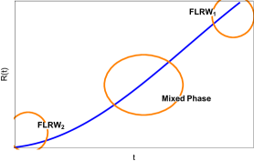
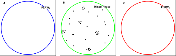
Figure 1: The upper plot represents two different initial and final FLRW universes. The plots A and C represent two different initial and final homogeneous universes while the plot B denotes growing inhomogeneities in the intermediate mixed phase.

$(iv)$

An important consequence of the phase transition between FLRW₂ and FLRW₁ is the topology change in the universe. Since FLRW₂ dominating at early times and FLRW₁ dominating at late times have different spatial curvatures in general, the universe may undergo a topology change from $k_{2}$ to $k_{1}$ during its evolution. For this topological transition, one realizes the following two points.

$1.$

If $k_{1}\geq 0$ and $k_{2}>0$ (or $k_{1}>0$ and $k_{2}\geq 0)$, hence $r\in[0,\infty)$. This case represents the topology change from a closed universe to another flat or closed universe (or vice versa). To observe this topology change, considering $k_{1}\geq 0$ and $k_{2}>0$ in (4.2), we have

$$c(t,r)=\frac{\sqrt{R(t)}}{\sqrt{1+k_{1}r^{2}}}+\frac{\gamma}{\sqrt{R(t)}}\frac{1}{\sqrt{1+k_{2}r^{2}}}.$$ (5.1)

The dominant term in $c(t,r)$ at the asymptotic limit $t\to 0$ and thus $R(t)\to 0$ is the second term with the topology $k_{2}>0$. As time progresses toward the late times, i.e as $t\to\infty$ and thus $R(t)\to\infty$, the first term in (5.1) with the topology $k_{1}\geq 0$ dominates and consequently a change of topology occurs.

$2.$

If $k_{1}\geq 0$ and $k_{2}<0$ or ($k_{1}<0$ and $k_{2}\geq 0$). This case represents a topology change from a spatially open to a flat or closed universe (or vice versa). To observe the topology change in this case, we have

$$c(t,r)=\frac{\sqrt{R(t)}}{\sqrt{1+k_{1}r^{2}}}+\frac{\gamma}{\sqrt{R(t)}}\frac{1}{\sqrt{1-|k_{2}|r^{2}}}.$$ (5.2)

Here, there is a restriction on the coordinate patch as $r\in[0,\frac{1}{\sqrt{|k_{2}|}})$. If $k_{1}=0$, in the asymptotic limit $t\to 0$ and hence $R(t)\to 0$, regardless of whatever $r$ is, the second term in (5.2) dominates. Then, at the early time asymptotic state, the topology is $k_{2}<0$. At the late times, there are two possibilities as $(i)$ in the region $0\leq r\ll\frac{1}{\sqrt{|k_{2}|}}$, as $t\to\infty$ and $R(t)\to\infty$, the first term in (2) dominates and a topology change occurs in time. In this region, the universe starts with the open topology $k_{2}<0$ and evolves toward the state with a flat topology $k_{1}=0$, and $(ii)$ in the asymptotic region, i.e. $r\to\frac{1}{\sqrt{|k_{2}|}}$, the second term survives in the limit $t\to\infty$ and $R(t)\to\infty$. Thus, both the terms in (5.2) can be effective that preserves the inhomogeneity at the asymptotic region. For this case, the topological structure of the asymptotic region can be more complicated than the previous cases and it may be different than both of the $k_{1}$ and $k_{2}$. It is interesting that here the topologies for the internal and asymptotic regions of spacetime can be different which implies another kind of topology change. A similar topology change occur also for $k_{1}<0$ and $k_{2}\geq 0$. In particular, the case $k_{1}<0$ and $k_{2}>0$ represents the topology change of the spacetime akin to the "bag of gold" geometry of Wheeler [21].

A Particular Example: Initially inflating and finally accelerating expanding universe scenario

Considering the scale factor $R(t)=R_{0}\left(e^{\sqrt{\frac{\Lambda}{3}}t}-1\right)$, one observes that in the early universe as $R(t)\to 0$, FLRW₂ (4.8) dominates in the superposition. Then, the evolution of the universe is governed by (4.10) and (4.11). According to (4.10) and (4.11), we have $\rho_{2}(t)\to\infty$ and $p_{2}(t)\to-\infty$ as $t\to 0$, respectively. The first represents the initial singularity in the matter sector while the latter represents a self driven inflation in the early times. It the late times, as $t\to\infty$, $R(t)\to R_{0}e^{\sqrt{\frac{\Lambda}{3}}t}$, FLRW₁ (4.8) is dominant in the superposition and the universe evolves according to (4.6) and (4.7) to an accelerating expanding a pure de Sitter phase, i.e. $\rho_{1}(t)\to 0$ and $p_{1}(t)\to 0$ as $t\to\infty$. Then, one observes an interesting property in this exact solution to the Einstein field equations. Indeed, this solution provides a scenario including the early time inflation, inhomogeneous structure formation in the intermediate era, and the late time accelerating expansion in a unified model possessing a possible topology change. In the intermediate phase where both FLRW₁ and FLRW₂ contribute effectively to the evolution of the universe, the inhomogeneities emerge. This possibility cannot be achieved in the usual standard FLRW cosmology with only time dependent field equations. One may argue about the physical nature of the solution by addressing the matter density, pressure and energy conditions. In Figure 2, we have plotted the density $\rho(t,r)$ and pressure $p(t,r)$ in (2.4) and (2.5), respectively, as well as $\sigma(t,r)=\rho+p$ for some typical values of the parameters. It is seen that for a superposed universe undergoing a topology change from a closed to flat topology with the scale factor $R(t)=R_{0}\left(e^{\sqrt{\frac{\Lambda}{3}}t}-1\right)$, there are regions where the density remains positive and pressure and $\sigma$ are negative. The negativeness of $\sigma$ represents the violation of weak energy condition that is consistent with the expanding nature of the cosmos in the context of this solution.

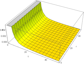
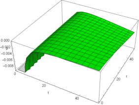
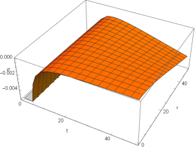
Figure 2: The evolution of the density $\rho(t,r)$, pressure $p(t,r)$ and $\sigma(t,r)=\rho+p$, respectively, for the parameter values $k_{1}=0,\,k_{2}=1,\,\gamma=1,\,R_{0}=1,\,\sqrt{\Lambda/3}=0.0001$, and $R(t)=R_{0}\left(e^{\sqrt{\frac{\Lambda}{3}}t}-1\right)$.

5.2 Cyclic universe scenarios

There are various cyclic universe scenarios, as exemplified in [14, 15, 16]. The old cyclic scenario is based on the possibility that the scale factor $R(t)$ of the universe oscillates at regularly spaced intervals of time between maximum and minimum values [14]. Considering such a scale factor, the superposed universe may undergo a topology change during each of its expansion and contraction phases between those minimum and maximum values of the scale factor $R(t)$, see Figure 3. As the scale factor reaches its minimum and maximum values, the universe becomes approximately homogeneous FLRW₂ and FLRW₁, respectively, and it is in the mixed phase between these extremum points where inhomogeneities emerge.

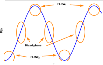
Figure 3: The evolution of a cyclic universe undergoing a topology change during the oscillation between subsequent global maximum and minimum values of its scale factor $R(t)$.

Another possible type of cyclic universe scenario was proposed recently by Ijjas and Steinhardt [15]. In this model, instead of the scale factor $R(t)$, the Hubble parameter $H(t)=\dot{R}(t)/R(t)$ oscillates periodically during the evolution of the universe. In the context of this model, the scale factor $R(t)$ increases substantially during each cosmological era and then undergoes an ultra-slow contraction phase at the end of each cycle. Then, the next cycle of the universe begins with a non-singular bounce. Figure 4 represents a typical plot of this type of cyclic universe scenario. In the first cycle, from $t_{0}$ to $t_{2}$, the universe expands from FLRW₂ at $t_{0}$ with the spatial curvature $k_{2}$ to FLRW₁ at the local maximum of $R(t)$ at $t_{1}$ with the spatial curvature of $k_{1}$. Then, it contracts between $t_{1}$ to $t_{2}$ and recover its previous curvature $k_{2}$ of the FLRW₂ state provided that $R_{2}\ll R_{1}$. In both the expansion and contraction phases, the universe becomes inhomogeneous in between the local maximum and minimum values of the scale factor. One also notes that by flattening the contraction phases, i.e. in the second cycle where $R_{3}\sim R_{4}$, the universe keeps its topology in the contraction phase as in the past local maximum point but still evolves inhomogeneously toward the non-singular bouncing point.

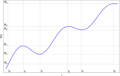
Figure 4: The evolution of a cyclic universe undergoing a topology change in transition through the local maximum and minimum values of a typical scale factor $R(t)=e^{\lambda t}J^{2}_{0}(t)+4$ where $J_{0}$ is the zeroth order Bessel function and we have set the dimensionless parameter $\lambda=0.009$.

As a final remark, let us note that although in Penrose’s conformal cyclic cosmological picture [16] there is no contraction phase, since in each aeon the universe is ever expanding ($R(t_{f})\gg R(t_{i})$ where $i$ and $f$ denote the initial and final states of an arbitrary aeon) the universe undergoes a change of spatial curvature from $k_{2}$ to $k_{1}$ during the evolution of each aeon. This requires a sudden change of spatial curvature and possibly topology change at the transition point from the past aeon to the present aeon from $k_{1}$ to $k_{2}$. This sudden transition point corresponds to the Big Bang of the present aeon. However, since the metric of the past aeon at its null infinity and the metric of the present aeon at its Big Bang surface are conformally related, occurrence of such a sudden topology change is forbidden in the conformal cyclic cosmology picture.

6 Conclusions

A summary of what we propose in this work is as follows: (1) we give a new example of nonlinear superposition in general relativity. This is a superposition of two different homogenous FLRW universes yielding an inhomogeneous cosmological model. (2) The metric is invariant under the scale factor inversion. (3) If the scale factor $R$ is zero in the beginning of the universe and goes to infinity as $t\to\infty$ then the universe starts approximately as a FLRW universe and ends as a different FLRW universe. (4) During such a phase transition the spatial curvature of 3-space changes in both magnitude and sign. If the sign changes then the topology of the 3-space also changes but if the sign remains intact, then the spatial curvature of the 3-space either increases or decreases.

References

- [1] M. Gürses and Y. Heydarzade, New Classes of Spherically Symmetric, Inhomogeneous Cosmological Models, Phys. Rev. D 100, 064048 (2019).
- [2] P. Kustaanheimo and B. Qvist, Societas Scientiarum Fennicae Commentationes Physico-Mathematicae XIII no. 16, 1 (1948), A. Krasinski, Editor’s Note: A Note on Some General Solutions of the Einstein Field Equations in a Spherically Symmetric World, paper reprinted in Gen. Relativ. Gravit. 30, 663 (1998); V. S. Brezhnev, Problemy teorii gravitatsii i elementarnykh chastits (Problems of Gravitation Theory and Elementary Particle Theory), 1st edition, Edited by K. P. Stanyukovich and G. A. Sokolnik. Atomizdat, Moskva, 158 (1966); V. S. Brezhnev, D. Ivanenko, and V. N. Frolov, Izv. VUZ Fiz. 9 no. 6, 119 (1966); E. N. Glass and B. Mashhoon, On a spherical star system with a collapsed core, Astrophys. J. 205, 570 (1976); N. Chakravarty, S. B. Dutta Choudhury and A. Banerjee, Nonstatic Spherically Symmetric Solutions for a Perfect Fluid in General Relativity, Austral. J. Phys. 29, 113 (1976); H. Knutsen, Regular exact models for a nonstatic gas sphere in general relativity, Gen. Rel. Grav. 17, 1121 (1985); H. Knutsen, Exact model for a gaseous regular bouncing sphere in general relativity, Int. J. Theor. Phys. 26, 895 (1987).
- [3] A. Krasinski, Inhomogeneous Cosmological Models (Cambridge University Press, Cambridge, England 1997).
- [4] K. Bolejko, M.-N. Cellerier and A. Krasinski, Inhomogeneous cosmological cosmological models: Exact solutions and their applications, Class. Qunatum Gravity 28, 164002 (2011).
- [5] G.C. McVittie, The mass-particle in an expanding universe, Mon. Not. R. Atrop. Soc. 93, 325 (1933).
- [6] P. C. Vaidya and Y. P. Shah, The gravitational field of a charged particle embedded in an expanding universe, Curr. Sci. 36, 120 (1967); Y. P. Shah and P. C. Vaidya, Gravitational field of a charged particle embedded in a homogeneous universe, Tensor 19, 191 (1968); P. C. Vaidya, The Kerr metric in cosmological background, Pramana 8, 512 (1977).
- [7] V. Faraoni, Evolving Black Hole Horizons in General Relativity and Alternative Gravity, Galaxies 1, 114-179 (2018).
- [8] N. Kaloper, M. Kleban, and D. Martin, McVittie’s legacy: Black holes in expanding universe, Phys. Rev. D 81, 104044 (2010); K. Lake and M. Abdelqader, More on McVittie’s legacy: A Schwarzschild-de Sitter black hole and white hole embedded in an asymptotically cosmology, Phys. Rev. D 84, 044045 (2011).
- [9] F. J. Chinea, New Bäcklund Transformations and Superposition Principle for Gravitational Fields with Symmetries, Phys. Rev. Lett. 50, 221 (1983).
- [10] F. J. Chinea, Vector Bäcklund Transformations and Associated Superposition Principle, in Solutions of Einstein’s Equations; Techniques and Results, Edited by C. Hoensalears and W. Dietz, Lecture Notes in Physics, No. 205, pp. 55-67, Springer, Berlin, (1984).
- [11] M. Gürses, Gravitational One Solitons, Phys. Rev. Lett. 51, 1810 (1983).
- [12] M. Gürses, Inverse Scattering, Differetial Geometry, Einstein Maxwell 2N Solitons and Gravitational One Soliton Bäcklund Transformations in Solutions of Einstein’s Equations; Techniques and Results, Edited by C. Hoensalears and W. Dietz , Lecture Notes in Physics, No. 205, pp. 199-234, Springer, Berlin, (1984).
- [13] N. Turok, P. Bhattacharjee, Stretching cosmic strings, Physical Review D, 29 (8), 1557 (1984); H.J. De Vega and N. Sanchez, Phys. Lett. B 197, 322 (1987), A new approach to string quantization in curved spacetimes; G. Veneziano, Scale factor duality for classical and quantum strings, Phys. Lett. B 265, 287 (1991); M. Gasperini and G. Veneziano, The pre-big bang scenario in string cosmology, Phys. Rept. 373, 1 (2003).
- [14] A. Friedmann, On the curvature of space Z. Phys. 10, 377 (1922); R.C. Tolman and M. Ward, On the behavior of non-static models of the universe when the cosmological term is omitted, Phys. Rev. 39, 835 (1932).
- [15] A. Ijjas and P. Steinhardt, A new kind of cyclic universe, Phys. Lett. B 795, 666 (2019).
- [16] R. Penrose, The basic ideas of conformal cyclic cosmology, AIP Conference Proceedings 11, 1446, 1 (2012); R. Penrose, On the gravitization of quantum mechanics 2: Conformal cyclic cosmology, Foundations of Physics, 44(8), 873 (2014); V.G. Gurzadyan and R. Penrose, On CCC-predicted concentric low-variance circles in the CMB sky, The European Physical Journal Plus 128, 22 (2013); V.G. Gurzadyan and R. Penrose, CCC and the Fermi paradox, The European Physical Journal Plus 131, 11 (2016); R. Penrose, The Big Bang and its Dark-Matter Content: Whence, Whither and Wherefore, Found. Phys. 48, 1177 (2018).
- [17] R. Penrose, Singularities in Cosmology, Confrontation of cosmological theories with Observational Data, M. S. Langair (Ed.), 563 (1974).
- [18] J. D. Barrow, S. Cotsakis, and A. Tsokaros, A general sudden cosmological singularity, Class. Quantum Gravity, 27, 165017 (2010).
- [19] J. D. Barrow and S. Cotsakis, Geodesics at sudden singularities, Phys. Rev. D 88, 067301 (2013).
- [20] K. Lake, Sudden future singularities in FLRW cosmologies, Class. Quantum Gravity 21, L 129 (2004).
- [21] J. A. Wheeler, in Les Houches Summer Shcool of Theoretical Physics: Relativity, Groups and Topology, Gordon and Breach Science Publishers, New York (1964).