Limit theorems for loop soup random variables

Abstract

This article deals with limit theorems for certain loop variables for loop soups whose intensity approaches infinity. We first consider random walk loop soups on finite graphs and obtain a central limit theorem when the loop variable is the sum over all loops of the integral of each loop against a given one-form on the graph. An extension of this result to the noncommutative case of loop holonomies is also discussed. As an application of the first result, we derive a central limit theorem for windings of loops around the faces of a planar graphs. More precisely, we show that the winding field generated by a random walk loop soup, when appropriately normalized, has a Gaussian limit as the loop soup intensity tends to $\infty$, and we give an explicit formula for the covariance kernel of the limiting field. We also derive a Spitzer-type law for windings of the Brownian loop soup, i.e., we show that the total winding around a point of all loops of diameter larger than $\delta$, when multiplied by $1/\log\delta$, converges in distribution to a Cauchy random variable as $\delta\to 0$.

1 Introduction

Windings of Brownian paths have been of interest since Spitzer’s classic result [Spi58] on their asymptotic behavior which states that, if $\theta(t)$ is the winding angle of a planar Brownian path about a point, then $2(\log t)^{-1}\theta(t)$ converges weakly to a Cauchy random variable as $t\rightarrow\infty$. The probability mass function for windings of any planar Brownian loop was computed in [Yor80] (see also [LJ18]), and similar results for random walks were obtained in [SY11]. Windings of simple random walks on the square lattice were more recently studied in [Bud17, Bud18].

Symanzik, in his seminal work on Euclidean quantum field theories [Sym69], introduced a representation of a Euclidean field as a “gas” of (interacting) random paths. The noninteracting case gives rise to a Poissonian ensemble of Brownian loops, independently introduced by Lawler and Werner [LW04] who called it the Brownian loop soup. Its discrete version, the random walk loop soup was introduced in [LF07].

Integrals over one-forms for loops ensembles, which are generalizations of windings, were considered in [LJ11, Chapter-6]. Various topological aspects of loop soups, such as homotopy and homology, were studied in [LJ19]. In [CGK16], the n-point functions of fields constructed taking the exponential of the winding numbers of loops from a Brownian loop soups are considered. The fields themselves are, a priori, only well-defined when a cutoff that removes small loops is applied, but the n-point functions are shown to converge to conformally covariant functions when the cutoff is sent to zero. A discrete version of these winding fields, based on the random walk loop soup, was considered in [BCL18]. In that paper, the n-point functions of these discrete winding fields are shown to converge, in the scaling limit, to the continuum n-point functions studied in [CGK16]. The same paper contains a result showing that, for a certain range of parameters, the cutoff fields considered in [CGK16] converge to random generalized functions with finite second moments when the cutoff is sent to zero. A similar result was established later in [LJ18] using a different normalization and a different proof.

In this article, we focus mainly on loop ensembles on graphs (see [LJ11] for an introduction and various results on this topic), except for Section 4, which deals with windings of the Brownian loop soup. In Section 2, we establish a central limit theorem for random variables that are essentially sums of integrals of a one-form over loops of a random walk loop soup, as the intensity of the loop soup tends to infinity. In Section 3 we apply the results of Section 2 to the winding field generated by a random walk loop soup on a finite graph and on the infinite square lattice. Finally, in Section 5, we discuss an extension of this results of Section 2 to the noncommutative case of loop holonomies.

2 A central limit theorem for loop variables

Let $\mathcal{G}=(X,E)$ be a finite connected graph and, for any vertices $x,y\in X$, let $d(x,y)$ denote the graph distance between $x$ and $y$ and $d_{x}$ the degree of $x$. The transition matrix $P$ for the random walk on the graph $\mathcal{G}$ with killing function $\kappa:X\rightarrow[0,\infty)$ is given by

$$P_{xy}=\begin{cases}\frac{1}{\kappa_{x}+d_{x}}&\text{ if }d(x,y)=1,\\ 0&\text{ otherwise.}\end{cases}$$ (1)

Let $G=(I-P)^{-1}$ denote the Green’s function corresponding to $P$. $G$ is well defined as long as $\kappa$ is not identically zero.

We call a sequence $\{x_{0},x_{1},\dots,x_{n},x_{n+1}\}$ of vertices of $\mathcal{G}$ with $d(x_{i},x_{i+1})=1$ for every $i=0,\dots,n$ and with $x_{n+1}=x_{0}$ a rooted loop with root $x_{0}$ and denote it by $\gamma_{r}$. To each $\gamma_{r}$ we associate a weight $w_{r}(\gamma_{r})=\frac{1}{n+1}P_{x_{0}x_{1}}\dots P_{x_{n}x_{0}}$. For a rooted loop $\gamma_{r}=\{x_{i}\}$, we interpret the index $i$ as time and define an unrooted loop as an equivalence class of rooted loops in which two rooted loops belong to the same class if they are the same up to a time translation. To an unrooted loop $\gamma$ we associate a weight $\mu(\gamma)=\sum_{\gamma_{r}\in\gamma}w_{r}(\gamma_{r})$. The random walk loop soup $\mathcal{L}^{\lambda}$ with intensity $\lambda>0$ is a Poissonian collection of unrooted loops with intensity measure $\lambda\mu$.

A one-form on $\mathcal{G}$ is a skew-symmetric matrix $A$ with entries $A_{xy}=-A_{yx}$ if $d(x,y)=1$ and $A_{xy}=0$ otherwise. A special case of $A$ is illustrated in Figure 1. For any (rooted/unrooted) loop $\gamma=\{x_{0},x_{1},\dots,x_{n},x_{0}\}$, denote

$$\int\limits_{\gamma}A=A_{x_{0},x_{1}}+A_{x_{1},x_{2}}+\dots+A_{x_{n},x_{0}}.$$

Given a one-form $A$ and a parameter $\beta\in{\mathbb{R}}$, we define a ‘perturbed transition matrix’ $P^{\beta}$ with entries

$$P_{xy}^{\beta}=\begin{cases}\frac{e^{i\beta A_{xy}}}{\kappa_{x}+d_{x}}&\text{ if }d(x,y)=1,\\ 0&\text{ otherwise.}\end{cases}$$ (2)

Note that $P^{\beta}=P$ when $\beta=0$.

Our aim is to derive a central limit theorem for the loop soup random variable

$$\int\limits_{\mathcal{L}^{\lambda}}A=\sum\limits_{\gamma\in\mathcal{L}^{\lambda}}{\int\limits_{\gamma}A}$$

as the intensity $\lambda$ of the loop soup increases to infinity. The key to prove such a result is the following representation of the characteristic function of $\int\limits_{\mathcal{L}^{\lambda}}A$.

Lemma 1.

With the above notation, assuming that $\kappa$ is not identically zero, we have that

$$\mathbb{E}_{\mathcal{L}^{\lambda}}\left[e^{\left(i\beta\int\limits_{\mathcal{L}^{\lambda}}A\right)}\right]=\left(\frac{\det(I-P^{\beta})}{\det(I-P)}\right)^{-\lambda}.$$

Proof.

Note that $\det(I-P^{\beta})^{\lambda}$ is well defined and can be written as $e^{\lambda\log\det(I-P^{\beta})}=e^{\lambda\operatorname{Tr}\log(I-P^{\beta})}$. Since $\kappa$ is not identically $0$, the spectral radius of $P^{\beta}$ is strictly less than $1$, which implies that

$$-\log(I-P^{\beta})=\sum\limits_{k=1}^{\infty}\frac{(P^{\beta})^{k}}{k},$$

where the series in the above expression is convergent.

The weight of all loops of length $k\geq 2$ is given by $\frac{1}{k}\operatorname{Tr}(P^{k})$. Therefore the measure of all loops of arbitrary length is

$$\sum\limits_{k=2}^{\infty}\frac{1}{k}\operatorname{Tr}(P^{k})=-\operatorname{Tr}\log(I-P)=-\log\det(I-P).$$

Similarly, we have

$$\int e^{i\beta\int\limits_{\gamma}A}d\mu(\gamma)=\sum\limits_{k=2}^{\infty}\frac{1}{k}\operatorname{Tr}((P^{\beta})^{k})=-\log\det(I-P^{\beta}).$$

Therefore, invoking Campbell’s theorem for point processes, we have that

$$\mathbb{E}_{\mathcal{L}^{\lambda}}\left[e^{\left(i\beta\sum\limits_{\gamma\in\mathcal{L}^{\lambda}}{\int\limits_{\gamma}A}\right)}\right]=e^{\left(\lambda\int[\exp{(i\beta\int\limits_{\gamma}A)}-1]d\mu(\gamma)\right)} =\frac{\det(I-P^{\beta})^{-\lambda}}{\det(I-P)^{-\lambda}},$$

which concludes the proof. ∎

A way to interpret the lemma, which also provides an alternative proof, is to notice that $\det(I-P)^{-\lambda}$ is the partition function $Z_{\lambda}$ of the random walk loop soup on $\mathcal{G}$ with transition matrix $P$ and intensity $\lambda$, while $\det(I-P^{\beta})^{-\lambda}$ is the partition function $Z_{\lambda}^{\beta}$ of a modified random walk loop soup on $\mathcal{G}$ whose transition matrix is given by $P^{\beta}$. The expectation in Lemma 1 is given by $1/Z_{\lambda}=\det(I-P)^{\lambda}$ times the sum over all loop soup configurations $\mathcal{L}^{\lambda}$ of $\exp{\left(i\beta\sum\limits_{\gamma\in\mathcal{L}^{\lambda}}{\int\limits_{\gamma}A}\right)}$ times the weight of $\mathcal{L}^{\lambda}$. The factor $\exp{\left(i\beta\sum\limits_{\gamma\in\mathcal{L}^{\lambda}}{\int\limits_{\gamma}A}\right)}$ can be absorbed into the weight of $\mathcal{L}^{\lambda}$ to produce a modified weight corresponding to a loop soup with transition matrix $P^{\beta}$. Therefore the sum mentioned above gives the partition function $Z_{\lambda}^{\beta}=\det(I-P^{\beta})^{-\lambda}$. Other interpretations of the quantity in Lemma 1 will be discussed in the next section, after the proof of Lemma 2.

To state our next result, we introduce the Hadamard and wedge matrix product operations denoted by $\odot$ and $\wedge$, respectively. For any two matrices U and V of same size, the Hardamard product between them (denoted $U\odot V$) is given by the matrix (of the same size as $U$ and $V$) whose entries are the products of the corresponding entries in $U$ and $V$. The following is the only property of matrix wedge products that will be used in this article: If $\lambda_{1},\dots,\lambda_{n}$ are the eigenvalues of an $n\times n$ matrix $U$, then $\operatorname{Tr}(U^{\wedge k})=\sum\limits_{i_{1}<\dots<i_{k}}\lambda_{i_{1}}\dots\lambda_{i_{k}}$ for all $k\leq n$. Recall also that $G=(I-P)^{-1}$ denotes the Green’s function corresponding to $P$, which is well defined as long as the killing function $\kappa$ is not identically zero.

Theorem 1.

With the above notation, assuming that $\kappa$ is not identically zero, the distribution of the random variable $\frac{1}{\sqrt{\lambda}}\int\limits_{\mathcal{L}^{\lambda}}A=\frac{1}{\sqrt{\lambda}}\sum\limits_{\gamma\in\mathcal{L}^{\lambda}}{\int\limits_{\gamma}A}$ tends to a Gaussian distribution as $\lambda\to\infty$. More precisely,

$$\lim\limits_{\lambda\rightarrow\infty}\mathbb{E}_{\mathcal{L}^{\lambda}}\left[e^{\left(i\frac{s}{\sqrt{\lambda}}\int\limits_{\mathcal{L}^{\lambda}}A\right)}\right]=\exp{\Big{[}-\frac{s^{2}}{2}\Big{(}\operatorname{Tr}\big{(}(P\odot A^{\odot 2})G\big{)}-\operatorname{Tr}\big{(}(P\odot A)G(P\odot A)G\big{)}\Big{)}\Big{]}}.$$

Proof.

Let $E^{\beta}=P-P^{\beta}$, then

$$E_{xy}^{\beta}=\begin{cases}\frac{1-e^{i\beta A_{xy}}}{\kappa_{x}+d_{x}}&\text{ if }d(x,y)=1,\\ 0&\text{ otherwise.}\end{cases}$$

Invoking Lemma 1, we have that

$$\mathbb{E}_{\mathcal{L}^{\lambda}}\left[e^{\left(i\beta\sum\limits_{\gamma\in\mathcal{L}^{\lambda}}\int\limits_{\gamma}A\right)}\right] = \left(\frac{\det(I-P^{\beta})}{\det(I-P)}\right)^{-\lambda}$$

$$= \left(\frac{\det(I-P+E^{\beta})}{\det(I-P)}\right)^{-\lambda},$$

$$= \left(\det(I-P)^{-1}(I-P+E^{\beta})\right)^{-\lambda},$$

$$= \left(\det(I+(I-P)^{-1}E^{\beta})\right)^{-\lambda},$$

$$= \left(\det(I+GE^{\beta})\right)^{-\lambda}.$$

Let $M$ be a square matrix of dimension $n$ and $\|M\|$ denote the operator norm of $M$. Then,

$$\det(I+M) =1+\operatorname{Tr}(M)+\operatorname{Tr}(M\wedge M)+\dots+\operatorname{Tr}(M^{\wedge n})$$ (3)

and

$$|\operatorname{Tr}(M^{\wedge k})| \leq{n\choose k}\|M\|^{k}.$$ (4)

Using this, we can write

$$\left(\det(I+GE^{\beta})\right)^{-\lambda}=(1+\operatorname{Tr}(GE^{\beta})+\operatorname{Tr}(GE^{\beta}\wedge GE^{\beta})+O(\beta^{3}\|A\|^{3}))^{-\lambda},$$

which leads to

$$\lim\limits_{\begin{subarray}{c}\lambda\rightarrow\infty\end{subarray}}\mathbb{E}_{\mathcal{L}^{\lambda}}\Big{[}\exp{\Big{(}i\frac{s}{\sqrt{\lambda}}\sum\limits_{\gamma\in\mathcal{L}^{\lambda}}\int\limits_{\gamma}A\Big{)}}\Big{]}$$ (5)

$$=\lim\limits_{\begin{subarray}{c}\lambda\rightarrow\infty\end{subarray}}\left(1+\operatorname{Tr}(GE^{\frac{s}{\sqrt{\lambda}}})+\operatorname{Tr}(GE^{\frac{s}{\sqrt{\lambda}}}\wedge GE^{\frac{s}{\sqrt{\lambda}}})+O\left(\lambda^{\frac{-3}{2}}\right)\right)^{-\lambda}$$ (6)

$$=\lim\limits_{\begin{subarray}{c}\lambda\rightarrow\infty\end{subarray}}\exp{\left(-\lambda\log\left(1+\operatorname{Tr}(GE^{\frac{s}{\sqrt{\lambda}}})+\operatorname{Tr}(GE^{\frac{s}{\sqrt{\lambda}}}\wedge GE^{\frac{s}{\sqrt{\lambda}}})+O\left(\lambda^{\frac{-3}{2}}\right)\right)\right)}.$$ (7)

To preceed, note that $\operatorname{Tr}(GE^{\beta}\wedge GE^{\beta})=\frac{1}{2}(\operatorname{Tr}^{2}(GE^{\beta})-\operatorname{Tr}(GE^{\beta}GE^{\beta}))$. Moreover, using the identities $G_{xy}P_{yx}=G_{yx}P_{xy}$ and $A_{xy}=-A_{yx}$ several times, one gets

$$\operatorname{Tr}(GE^{\beta}) =\sum\limits_{x\thicksim y}G_{xy}E^{\beta}_{yx}$$ (8)

$$=\frac{1}{2}\sum\limits_{x\thicksim y}(G_{xy}E^{\beta}_{yx}+G_{yx}E^{\beta}_{xy}),$$ (9)

$$=\frac{1}{2}\sum\limits_{x\thicksim y}G_{xy}P_{yx}(1-e^{i\beta A_{yx}})+G_{yx}P_{xy}(1-e^{i\beta A_{xy}}),$$ (10)

$$=\sum\limits_{x\thicksim y}G_{xy}P_{yx}(1-\cos(\beta A_{yx})).$$ (11)

Therefore,

$$\operatorname{Tr}(GE^{\frac{s}{\sqrt{\lambda}}A}) =\frac{s^{2}}{2\lambda}\sum\limits_{x\thicksim y}G_{xy}P_{yx}A_{yx}^{2}+O\left(\frac{1}{\lambda^{\frac{3}{2}}}\|A\|^{3}\right)$$ (12)

$$=\frac{s^{2}}{2\lambda}\operatorname{Tr}(G(P\odot A^{\odot 2}))+O\left(\frac{1}{\lambda^{\frac{3}{2}}}\|A\|^{3}\right).$$ (13)

Similarly,

$$\operatorname{Tr}(GE^{\beta}GE^{\beta}) =\sum\limits_{\begin{subarray}{c}x_{0},x_{1},x_{2},x_{3}\\ x_{0}\thicksim x_{1};x_{2}\thicksim x_{3}\end{subarray}}E^{\beta}_{x_{0},x_{1}}G_{x_{1}x_{2}}E^{\beta}_{x_{2},x_{3}}G_{x_{3}x_{0}},$$ (14)

$$=\sum\limits_{\begin{subarray}{c}x_{0},x_{1},x_{2},x_{3}\\ x_{0}\thicksim x_{1};x_{2}\thicksim x_{3}\end{subarray}}(1-e^{i\beta A_{x_{0}x_{1}}})(1-e^{i\beta A_{x_{2}x_{3}}})P_{x_{0}x_{1}}P_{x_{2}x_{3}}G_{x_{3}x_{0}}G_{x_{1}x_{2}},$$ (15)

$$=\sum\limits_{\begin{subarray}{c}x_{0},x_{1},x_{2},x_{3}\\ x_{0}\thicksim x_{1};x_{2}\thicksim x_{3}\end{subarray}}(i\beta A_{x_{0}x_{1}}+O(\beta^{2}\|A\|^{2}))(i\beta A_{x_{2}x_{3}}+O(\beta^{2}\|A\|^{2}))P_{x_{0}x_{1}}P_{x_{2}x_{3}}G_{x_{3}x_{0}}G_{x_{1}x_{2}},$$ (16)

$$=\sum\limits_{\begin{subarray}{c}x_{0},x_{1},x_{2},x_{3}\\ x_{0}\thicksim x_{1};x_{2}\thicksim x_{3}\end{subarray}}-\beta^{2}A_{x_{0}x_{1}}P_{x_{0}x_{1}}G_{x_{1}x_{2}}A_{x_{2}x_{3}}P_{x_{2}x_{3}}G_{x_{3}x_{0}}+O(\beta^{3}\|A\|^{3}),$$ (17)

$$=-\beta^{2}\operatorname{Tr}[(P\odot A)G(P\odot A)G]+O(\beta^{3}\|A\|^{3}).$$ (18)

Note that the expressions $\operatorname{Tr}(GE^{\frac{1}{\sqrt{\lambda}}})$ and $\operatorname{Tr}(GE^{\frac{1}{\sqrt{\lambda}}}\wedge GE^{\frac{1}{\sqrt{\lambda}}})$ are of the order $\frac{1}{\lambda}$. Using this fact, and expanding the logarithm in power series, the above computations give

$$\lim\limits_{\begin{subarray}{c}\lambda\rightarrow\infty\end{subarray}}-\lambda\log\bigg{(}1+\operatorname{Tr}(GE^{\frac{s}{\sqrt{\lambda}}})+\operatorname{Tr}(GE^{\frac{s}{\sqrt{\lambda}}}\wedge GE^{\frac{1}{\sqrt{\lambda}}})+O\left(\lambda^{\frac{-3}{2}}\right)\bigg{)}$$

$$\quad\quad\quad\quad\quad=\lim\limits_{\begin{subarray}{c}\lambda\rightarrow\infty\end{subarray}}\left(-\frac{s^{2}}{2}\operatorname{Tr}(G(P\odot A^{\odot 2}))-\frac{s^{2}}{2}\operatorname{Tr}[(P\odot A)G(P\odot A)G]+O(\lambda^{\frac{-1}{2}})\right)$$

$$=-\frac{s^{2}}{2}\operatorname{Tr}(G(P\odot A^{\odot 2}))-\frac{s^{2}}{2}\operatorname{Tr}[(P\odot A)G(P\odot A)G],$$

which concludes the proof. ∎

Remark 1.

It may be useful to note the following identity, which holds when $A$ is skew-symmetric and $P$ is symmetric:

$$\frac{1}{2}\sum\limits_{\begin{subarray}{c}x_{0}\thicksim x_{1}\\ x_{2}\thicksim x_{3}\end{subarray}}P_{x_{0}x_{1}}P_{x_{2}x_{3}}A_{x_{0}x_{1}}A_{x_{2}x_{3}}[G_{x_{0}x_{3}}G_{x_{1}x_{2}}-G_{x_{0}x_{2}}G_{x_{1}x_{3}}]=\operatorname{Tr}[(P\odot A)G(P\odot A)G].$$

We will use this identity in the proof of Theorem 2 in the next section.

3 Central limit theorem for the loop soup winding field at high intensity

The winding field generated by a loop soup on a planar graph $\mathcal{G}=(X,E)$ is defined on the faces $f$ of $\mathcal{G}$, which we identify with the vertices of the dual graph $\mathcal{G}^{*}=(X^{*},E^{*})$ (i.e., $f\in X^{*}$). Fix any face $f\in X^{*}$ and let $f_{0}=f,f_{1},\dots,f_{n}$ be a sequence of distinct faces of $\mathcal{G}$ that are nearest-neighbors in $\mathcal{G}^{*}$, with $f_{n}$ the infinite face. The sequence $f_{0},f_{1},\dots,f_{n}$ determines a directed path $p$ from $f$ to the infinite face. Let $e^{p}_{i}$ denote the edge between $f_{i}$ and $f_{i+1}$ oriented in such a way that it crosses $p$ from right to left. We let $\text{cut}(f)$ denote the collection of oriented edges $\{e^{f}_{i}\}_{i=0}^{n-1}$. (See the Figure 1 below for an example.) Note that $\text{cut}(f)$ depends on the choice of $p$, but since all $p$’s connecting $f$ to the infinite face are equivalent for our purposes, we don’t include $p$ in the notation.

Now take an oriented loop $\ell$ in $\mathcal{G}$ and assume that $\ell$ crosses $p$. In this case, we say that $\ell$ crosses $\text{cut}(f)$ and we call the crossing positive if $\ell$ crosses $p$ from right to left and negative otherwise. For an oriented loop $\ell$ in $\mathcal{G}$ and a face $f\in X^{*}$, we define the winding number of $\ell$ about $f$ to be

$$W_{\ell}(f) = \text{cut}(f) \ell$$ number of positive crossings of by

$$-\text{ number of negative crossings of $\text{cut}(f)$ by $\ell$}$$

for any choice of $\text{cut}(f)$. We note that $W_{\ell}(f)$ is well defined because the difference above is independent of the choice of $\text{cut}(f)$. (This is easy to verify and is left as an exercise for the interested reader.)

For a loop soup $\mathcal{L}^{\lambda}$, we define

$$W_{\lambda}=\{W_{\lambda}(f)\}_{f\in\mathcal{G}^{*}}=\Big{\{}\sum_{\ell\in\mathcal{L}^{\lambda}}W_{\ell}(f)\Big{\}}_{f\in\mathcal{G}^{*}}$$ (19)

to be the winding field generated by $\mathcal{L}^{\lambda}$.

Theorem 1 can be used to prove a CLT for the winding field $W_{\lambda}$, when properly normalized, as $\lambda\to\infty$. In order to use Theorem 1, we need a definition and a lemma. For any collection of faces $f_{1},\dots,f_{n}$ of $\mathcal{G}$ and any vector $\bar{t}=(t_{1},\ldots,t_{n})$, define a skew-symmetric matrix $A^{\bar{t}}$ as follows. For each $i=1,\ldots,n$, choose a cut from $f_{i}$ to the infinite face as described above and denote it $\text{cut}(f_{i})$. If $e=(x,y)$ is an edge of $\text{cut}(f_{i})$ with positive orientation set $A^{\bar{t}}_{xy}=t_{i}$; if $e=(x,y)$ is an edge of $\text{cut}(f_{i})$ with negative orientation set $A^{\bar{t}}_{xy}=-t_{i}$; otherwise set $A^{\bar{t}}_{xy}=0$. Note that one can write $A^{\bar{t}}$ as $A^{t_{1}}_{f_{1}}+\ldots+A^{t_{n}}_{f_{n}}$ where $A^{t_{i}}$ is a matrix such that $(A^{t_{i}}_{f_{i}})_{xy}=t_{i}$ if $(x,y)$ is in $\text{cut}(f_{i})$ and has positive orientation, $(A^{t_{i}}_{f_{i}})_{xy}=-t_{i}$ if $(x,y)$ is in $\text{cut}(f_{i})$ and has negative orientation, and $(A^{t_{i}}_{f_{i}})_{xy}=0$ if $(x,y)\notin\text{cut}(f_{i})$.

Lemma 2.

For any collection of faces $f_{1},\dots,f_{n}$ of $\mathcal{G}$, there exists a skew-Hermitian matrix $A^{\overline{t}}$ such that the characteristic function of the random vector $(W_{\lambda}(f_{1}),\ldots,W_{\lambda}(f_{n}))$ is given by

$$\mathbb{E}_{\mathcal{L}^{\lambda}}[e^{i\beta(t_{1}W_{\lambda}(f_{1})+\dots+t_{n}W_{\lambda}(f_{n}))}]=\mathbb{E}_{\mathcal{L}^{\lambda}}\left[e^{\left(i\beta\sum\limits_{\gamma\in\mathcal{L}^{\lambda}}{\int\limits_{\gamma}A^{\overline{t}}}\right)}\right].$$

Proof.

Using the matrices $A^{\bar{t}}$ describe above, the result follows immediately from the definition of winding number. ∎

The quantity in the lemma has several interpretations. Besides being the characteristic function of the random vector $(W_{\lambda}(f_{1}),\ldots,W_{\lambda}(f_{n}))$, it can be seen as the $n$-point function of a winding field of the type studied in [BCL18] (see also [CGK16] for a continuum version). Moreover, by an application of Lemma 1,

$$\mathbb{E}_{\mathcal{L}^{\lambda}}[e^{i(t_{1}W_{\lambda}(f_{1})+\dots+t_{n}W_{\lambda}(f_{n}))}]=\left(\frac{\det(I-P^{\bar{t}})}{\det(I-P)}\right)^{-\lambda},$$

where

$$P_{xy}^{\bar{t}}=\begin{cases}\frac{e^{iA^{\bar{t}}_{xy}}}{\kappa_{x}+d_{x}}&\text{ if }d(x,y)=1\\ 0&\text{ otherwise}\end{cases}$$ (20)

and $A^{\bar{t}}$ is one of the matrices described above. A standard calculation using Gaussian integrals shows that

$$Z^{\bar{t}}_{GFF}=\Pi_{x\in X}\Big{(}\frac{2\pi}{\kappa_{x}+d_{x}}\Big{)}^{1/2}\det(I-P^{\bar{t}})^{-1/2},$$

where $Z^{\bar{t}}_{GFF}$ is the partition function of the Gaussian Free Field (GFF) on $\mathcal{G}$ with Hamiltonian

$$H^{\bar{t}}(\varphi)=-\frac{1}{2}\sum_{(x,y)\in E}e^{iA^{\bar{t}}_{xy}}\varphi_{x}\varphi_{y}+\frac{1}{2}\sum_{x\in X}(\kappa_{x}+d_{x})\varphi_{x}^{2}.$$ (21)

Hence, $\mathbb{E}_{\mathcal{L}^{\lambda}}[e^{i(t_{1}W_{\lambda}(f_{1})+\dots+t_{n}W_{\lambda}(f_{n}))}]$ can be written as a ratio of partition functions, namely,

$$\mathbb{E}_{\mathcal{L}^{\lambda}}[e^{i(t_{1}W_{\lambda}(f_{1})+\dots+t_{n}W_{\lambda}(f_{n}))}]=\Big{(}\frac{Z^{\bar{t}}_{GFF}}{Z_{GFF}}\Big{)}^{2\lambda},$$

where $Z_{GFF}$ is the partition function of the ‘standard’ GFF obtained from (21) by setting $t_{1}=\ldots=t_{n}=0$.

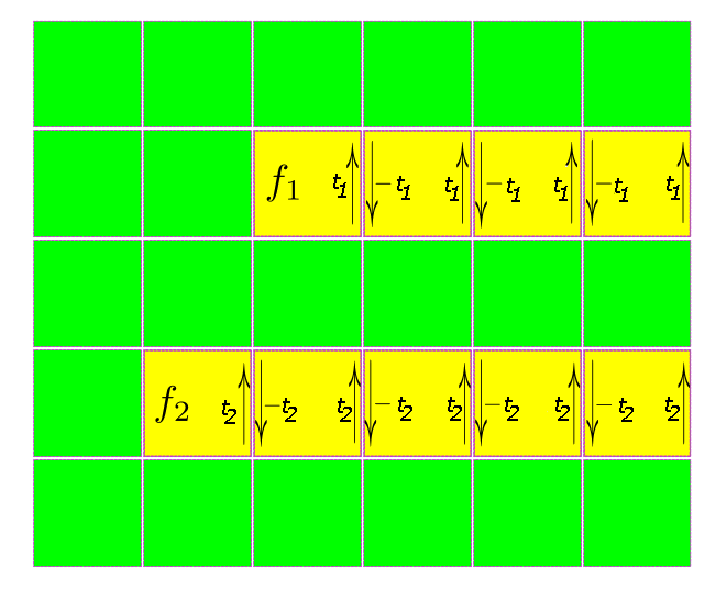
Figure 1: The above figure displays a choice of cuts for faces $f_{1}$ and $f_{2}$ in a rectangular grid graph.

To state the next theorem we need some additional notation. For any directed edge $e\in\text{cut}(f)$, let $e^{-}$ and $e^{+}$ denote the starting and ending vertices of $e$, respectively.

Theorem 2.

Consider a random walk loop soup on a finite graph $\mathcal{G}$ with symmetric transition matrix $P$ and the corresponding winding field $W_{\lambda}$. As $\lambda\rightarrow\infty$, $\frac{1}{\sqrt{\lambda}}W_{\lambda}$ converges to a Gaussian field whose covariance kernel is given by

$$K(f,g)= \sum\limits_{e\in\text{cut}(f)}P_{e^{+}e^{-}}G_{e^{+}e^{-}}\mathds{1}_{f=g}$$ (22)

$$+2\sum\limits_{\begin{subarray}{c}e_{1}\in\text{cut}(f)\\ e_{2}\in\text{cut}(g)\end{subarray}}P_{e_{1}^{+}e_{1}^{-}}P_{e_{2}^{+}e_{2}^{-}}\left(G_{e_{1}^{+}e_{2}^{-}}G_{e_{1}^{-}e_{2}^{+}}-G_{e_{1}^{+}e_{2}^{+}}G_{e_{1}^{-}e_{2}^{-}}\right)\mathds{1}_{f\neq g}.$$ (23)

Proof.

Combining Lemma 2 and Theorem 1 shows that the winding field has a Gaussian limit as $\lambda\to\infty$:

$$\Big{\{}\frac{1}{\sqrt{\lambda}}W_{\lambda}(f):f\text{ is a face of }\mathcal{G}\Big{\}}\xRightarrow[weakly]{\lambda\uparrow\infty}\Big{\{}W(f):f\text{ is a face of }\mathcal{G}\Big{\}}$$

where $W(\cdot)$ is a Gaussian process on the faces of $G$.

Next, we compute the covariance kernel of the limiting Gaussian process. Choose two faces $f$ and $g$ and let $A^{\overline{t}}=A^{t_{1}}_{f}+A^{t_{2}}_{g}$, where $A^{t_{1}}_{f}$ has nonzero entries only along $\text{cut}(f)$ and $A^{t_{2}}_{g}$ has nonzero entries along $\text{cut}(g)$, as described above. Using Theorem 1 we obtain

$$\lim\limits_{\lambda\rightarrow\infty} \log\mathbb{E}_{\mathcal{L}^{\lambda}}[e^{i\frac{1}{\sqrt{\lambda}}(t_{1}W_{\lambda}(f_{1})+t_{2}W_{\lambda}(f_{2}))}]$$ (24)

$$= -\frac{1}{2}\Big{[}\operatorname{Tr}((P\odot(A^{\overline{t}})^{\odot 2})G)+\operatorname{Tr}((P\odot A^{\overline{t}})G(P\odot A^{\overline{t}})G)\Big{]}$$ (25)

$$= -\frac{1}{2}\Big{[}\operatorname{Tr}((P\odot(A^{t_{1}}+A^{t_{2}})^{\odot 2})G)+\operatorname{Tr}((P\odot(A^{t_{1}}+A^{t_{2}}))G(P\odot(A^{t_{1}}+A^{t_{2}})G)\Big{]}$$ (26)

$$= -\frac{1}{2}\Big{[}t_{1}^{2}K(f,f)+t_{2}^{2}K(g,g)-2t_{1}t_{2}K(f,g)\Big{]}.$$ (27)

The variance of $W(f)$ is obtained by setting $t_{1}=t$ and $t_{2}=0$. In this case,

$$K(f,f) =\frac{1}{t^{2}}\Big{[}\operatorname{Tr}((P\odot(A^{t})^{\odot 2})G)+\operatorname{Tr}((P\odot A^{t})G(P\odot A^{t})G)\Big{]}$$ (28)

$$=\sum\limits_{e\in\text{cut}(f)}P_{e^{-}e^{+}}G_{e^{+}e^{-}}+\frac{1}{t^{2}}(\operatorname{Tr}((P\odot A^{t})G(P\odot A^{t})G)).$$ (29)

Since $P$ is assumed to be symmetric, the term $\operatorname{Tr}((P\odot A^{t})G(P\odot A^{t})G)$ vanishes. Therefore,

$$K(f,f)=\sum\limits_{e\in\text{cut}(f)}P_{e^{-}e^{+}}G_{e^{-}e^{+}}.$$

A similarly calculation, with $A^{\overline{t}}=A^{t_{1}}_{f}+A^{t_{2}}_{g}$, where $A^{t_{1}}_{f}$, gives the covariance:

$$K(f,g) = \frac{-1}{2t_{1}t_{2}}\Big{[}\operatorname{Tr}((P\odot(A^{t_{1}}+A^{t_{2}})^{\odot 2})G)+\operatorname{Tr}(P\odot(A^{t_{1}}+A^{t_{2}})G(P\odot(A^{t_{1}}+A^{t_{2}})G))$$

$$\quad-t_{1}^{2}K(f,f)-t_{2}^{2}K(g,g)\Big{]}$$

$$= \frac{-1}{2t_{1}t_{2}}\Big{[}\operatorname{Tr}((P\odot(A^{t_{1}}+A^{t_{2}})^{\odot 2})G)+\operatorname{Tr}(P\odot(A^{t_{1}}+A^{t_{2}})G(P\odot(A^{t_{1}}+A^{t_{2}})G))$$

$$\quad-\operatorname{Tr}((P\odot(A^{t_{1}})^{\odot 2})G)-\operatorname{Tr}((P\odot A^{t_{1}})G(P\odot A^{t_{1}})G)$$

$$\quad-\operatorname{Tr}((P\odot(A^{t_{2}})^{\odot 2})G)-\operatorname{Tr}((P\odot A^{t_{2}})G(P\odot A^{t_{2}})G)\Big{]}$$

$$= \frac{-1}{t_{1}t_{2}}\Big{[}\operatorname{Tr}((P\odot(A^{t_{1}}\odot A^{t_{2}}))G)+\operatorname{Tr}((P\odot A^{t_{1}})G(P\odot A^{t_{2}})G)\Big{]}.$$

Since $P$ is symmetric, $\operatorname{Tr}((P\odot(A^{t_{1}}\odot A^{t_{2}}))G)=0$ and, using Remark 1, we obtain

$$K(f,g)=2\sum\limits_{\begin{subarray}{c}e_{1}\in\text{cut}(f)\\ e_{2}\in\text{cut}(g)\end{subarray}}P_{e_{1}^{+}e_{1}^{-}}P_{e_{2}^{+}e_{2}^{-}}\left(G_{e_{1}^{+}e_{2}^{-}}G_{e_{1}^{-}e_{2}^{+}}-G_{e_{1}^{+}e_{2}^{+}}G_{e_{1}^{-}e_{2}^{-}}\right),$$

which concludes the proof. ∎

Remark 2.

We provide here an alternative, more direct, proof of Theorem 2. For any directed edge $e$, let $e^{-}$ and $e^{+}$ to denote the starting and ending vertices respectively. Moreover, let $N_{e}^{+}$ be the number of positive crossings of $e$ (i.e., from $e^{-}$ to $e^{+}$) by a loop from the loops soup and let $N_{e}^{-}$ be the number of negative crossings of $e$ (i.e., from $e^{+}$ to $e^{-}$) by a loop from the loops soup. The winding number about a face $f$ can be defined as,

$$W_{\lambda}(f)=\sum\limits_{e\in\text{cut}(f)}(N_{e}^{+}-N_{e}^{-}).$$

Therefore the two point function for the winding numbers is given by

$$\mathbb{E}_{\mathcal{L}^{1}}(W_{1}(f)W_{1}(g)) =\mathbb{E}_{\mathcal{L}^{1}}\Big{(}\sum\limits_{\begin{subarray}{c}e_{1}\in\text{cut}(f)\\ e_{2}\in\text{cut}(g)\end{subarray}}(N_{e_{1}}^{+}-N_{e_{1}}^{-})(N_{e_{2}}^{+}-N_{e_{2}}^{-})\Big{)}$$ (30)

$$=\mathbb{E}_{\mathcal{L}^{1}}\Big{(}\sum\limits_{\begin{subarray}{c}e_{1}\in\text{cut}(f)\\ e_{2}\in\text{cut}(g)\end{subarray}}(N_{e_{1}}^{+}N_{e_{2}}^{+}+N_{e_{1}}^{-}N_{e_{2}}^{-}-N_{e_{1}}N_{e_{2}}^{-}-N_{e_{1}}^{-}N_{e_{2}}^{+})\Big{)}$$ (31)

$$=2\sum\limits_{\begin{subarray}{c}e_{1}\in\text{cut}(f)\\ e_{2}\in\text{cut}(g)\end{subarray}}\left(\mathbb{E}_{\mathcal{L}^{1}}(N_{e_{1}}^{+}N_{e_{2}}^{+})-\mathbb{E}_{\mathcal{L}^{1}}(N_{e_{1}}^{+}N_{e_{2}}^{-})\right)$$ (32)

Using this expression and a result from [LJ11] (see [LJ11, Exercise 10, Chapter 2], but note that in [LJ11] the Green’s function is defined to be $[(I-P)^{-1}]_{x,y}/(\kappa_{y}+d_{y})=P_{yx}G_{xy}=P_{xy}G_{xy}$, when $P$ is symmetric), we obtain

$$\mathbb{E}_{\mathcal{L}^{1}} (W_{1}(f)W_{1}(g))$$ (33)

$$=\sum\limits_{\begin{subarray}{c}e_{1}\in\text{cut}(f)\\ e_{2}\in\text{cut}(g)\end{subarray}}\Big{(}P_{e_{2}^{+}e_{2}^{-}}P_{e_{1}^{+}e_{1}^{-}}G_{e_{1}^{+}e_{2}^{-}}G_{e_{2}^{+}e_{1}^{-}}+P_{e_{2}^{-}e_{2}^{+}}P_{e_{1}^{-}e_{1}^{+}}G_{e_{1}^{-}e_{2}^{+}}G_{e_{2}^{-}e_{1}^{+}}$$ (34)

$$\quad\quad\quad-P_{e_{2}^{-}e_{2}^{+}}P_{e_{1}^{+}e_{1}^{-}}G_{e_{1}^{+}e_{2}^{+}}G_{e_{2}^{-}e_{1}^{-}}-P_{e_{2}^{+}e_{2}^{-}}P_{e_{1}^{-}e_{1}^{+}}G_{e_{1}^{-}e_{2}^{-}}G_{e_{2}^{+}e_{1}^{+}}\Big{)}$$ (35)

$$=2\sum\limits_{\begin{subarray}{c}e_{1}\in\text{cut}(f)\\ e_{2}\in\text{cut}(g)\end{subarray}}P_{e_{1}^{+}e_{1}^{-}}P_{e_{2}^{+}e_{2}^{-}}\left(G_{e_{1}^{+}e_{2}^{-}}G_{e_{2}^{+}e_{1}^{-}}-G_{e_{1}^{+}e_{2}^{+}}G_{e_{2}^{-}e_{1}^{-}}\right).$$ (36)

Now take $\lambda=n\in{\mathbb{N}}$ and note that, for any face $f$, $W_{n}(f)$ is distributed like $\sum_{i=1}^{n}W_{1}^{i}(f)$, where $\{W_{1}^{i}(f)\}_{i=1,\ldots,n}$ are $n$ i.i.d. copies of $W_{1}(f)$. Therefore, for any collection of faces $f_{1},\dots,f_{m}$, the central limit theorem implies that, as $\lambda=n\to\infty$, the random vector $\frac{1}{\sqrt{n}}\left(W_{n}(f_{1}),\dots,W_{n}(f_{m})\right)$ converges to a multivariate Gaussian with covariance kernel given by the two-point function $\mathbb{E}_{\mathcal{L}^{1}}(W_{1}(f)W_{1}(g))$ calculated above.

Remark 3.

Theorem 2 can be extended to infinite graphs, as we now explain. For concreteness and simplicity, we focus on the square lattice and consider a random walk loop soup with constant killing function: $\kappa_{x}=\kappa>0$ for all $x\in{\mathbb{Z}}^{2}$. Note that in this case the transition matrix $P$ and the Green’s function $G$ are symmetric. Moreover, contrary to the case $\kappa=0$, the winding field of the random walk loop soup on ${\mathbb{Z}}^{2}$ is well defined when $\kappa>0$. To see this, note that, since the loop soup is a Poisson process, we can bound the expected number of loops intersecting $(-a,0),(b,0)\in{\mathbb{Z}}^{2}$ as follows:

$$\mathbb{E}_{\mathcal{L}^{\lambda}}\big{(}\#\text{ loops joining }(-a,0)\text{ and }(b,0)\big{)} = \lambda\mu\big{(}\gamma:\gamma(-a,0),(b,0)\in\gamma\big{)}$$

$$\leq \lambda\sum_{m\geq 2(a+b)}\Big{(}\frac{4}{\kappa+4}\Big{)}^{m}$$

$$= \frac{\lambda\kappa}{4}\Big{(}1+\frac{\kappa}{4}\Big{)}^{-2(a+b)}.$$

Hence, the expected number of loops winding around the origin is bounded above by $\frac{\lambda\kappa}{4}\sum_{a=1}^{\infty}\sum_{b=1}^{\infty}(1+\kappa/4)^{-2(a+b)}<\infty$ for any $\kappa>0$. This means that, with probability one, the number of loops winding around any vertex is finite. Because of this, one can obtain the winding field on ${\mathbb{Z}}^{2}$ as the weak limit of winding fields in large finite graphs $\mathcal{G}_{n}=[-n,n]^{2}\cap\mathbb{Z}^{2}$ as $n\to\infty$. It is now clear that one can apply the arguments in Remark 2 to the case of the winding field on $\mathbb{Z}^{2}$.

4 A Spitzer-type law for windings of the Brownian loop soup

Spitzer showed [Spi58] that the winding of Brownian motion about a given point up to time $t$, when scaled by $1/(2\log t)$, converges in distribution to a Cauchy random variable as $t\rightarrow\infty$. An analogous result for the simple symmetric random walk on ${\mathbb{Z}}^{2}$ is contained in Theorem 6 of [Bud18]. In this section we prove a similar result for the Brownian loop soup in a bounded domain.

Recall that the Brownian loop soup in a planar domain $D\subset{\mathbb{C}}$ is defined as a Poisson process of loops with intensity measure $\mu^{\text{loop}}$ given by

$$\mu^{\text{loop}}(\cdot)=\int\limits_{D}\int\limits_{0}^{\infty}\frac{1}{2\pi t^{2}}\mu_{\text{BB}}^{z,t}(\cdot)dtdA(z),$$

where $\mu_{\text{BB}}^{z,t}$ is the Brownian Bridge measure of time length $t$ starting at $z$ and $dA$ is the area measure on the complex plane (see [LW04] for a precise definition).

For any $z\in D$, we let $W^{\delta}_{\lambda}(z)$ denote the sum of the winding numbers about $z$ of all Brownian loops contained in $D$ with diameter at least $\delta$ for some $\delta>0$.

Theorem 3.

Consider a bounded domain $D\subset{\mathbb{C}}$. For any $z\in D$, as $\delta\rightarrow 0$, $\frac{W^{\delta}_{\lambda}(z)}{\log\delta}$ converges weakly to a Cauchy random variable with location parameter $0$ and scale parameter $\frac{\lambda}{2\pi}$.

Proof.

Let $d_{z}$ denote the distance between $z$ and the boundary of $D$ and, for $\delta<d_{z}$, let $W^{\delta,d_{z}}_{\lambda}(z)$ denote the sum of the winding numbers about $z$ of all Brownian loops with diameter between $\delta$ and $d_{z}$. Note that, because of the Poissonian nature of the Brownian loop soup, the random variables $W^{\delta,d_{z}}_{\lambda}(z)$ and $W^{d_{z}}_{\lambda}(z)$ are independent.

The key ingredient in the proof is Lemma 3.2 of [CGK16], which states, in our notation, that

$$\mathbb{E}\big{(}e^{i\beta W^{\delta,d_{z}}_{\lambda}(z)}\big{)}=\Big{(}\frac{d_{z}}{\delta}\Big{)}^{-\lambda\frac{\beta(2\pi-\beta)}{4\pi^{2}}}=d_{z}^{-\lambda\frac{\beta(2\pi-\beta)}{4\pi^{2}}}e^{\lambda\frac{\beta(2\pi-\beta)}{4\pi^{2}}\log\delta}$$

when $\beta\in[0,2\pi)$, and that the same expression holds with $\beta$ replaced by $(\beta\mod 2\pi)$ when $\beta\notin[0,2\pi)$. With this result, choosing $\beta=s/\log\delta$, the limit as $\delta\to 0$ of the characteristic function of $\frac{W^{\delta}_{\lambda}(z)}{\log\delta}$ can be computed as follows:

$$\lim_{\delta\to 0}\mathbb{E}\big{(}e^{i\frac{s}{\log\delta}W^{\delta}_{\lambda}(z)}\big{)}=\lim_{\delta\to 0}\mathbb{E}\big{(}e^{i\frac{s}{\log\delta}W^{\delta,d_{z}}_{\lambda}(z)}\big{)}\mathbb{E}\big{(}e^{i\frac{s}{\log\delta}W^{d_{z}}_{\lambda}(z)}\big{)}=e^{-\frac{\lambda}{2\pi}|s|},$$

where the right hand side is the characteristic function of a Cauchy random variable with location parameter $0$ and scale parameter $\frac{\lambda}{2\pi}$. ∎

5 Holonomies of loop ensembles

Theorem 1 can be generalized to loop holonomies. Assume that the transition matrix $P$ introduced at the beginning of Section 2 is symmetric and hence the Green’s function is also symmetric. We consider a connection on the graph $\mathcal{G}$, given by assigning to each oriented edge $(x,y)$ a $d\times d$ unitary matrix $\bf{U}_{xy}$ of the form $U_{xy}=e^{iA_{xy}}$ for some Hermitian matrix $A_{xy}$. For any closed loop $\gamma=\{x_{0},x_{1},\dots,x_{n},x_{0}\}$, we denote

$$\prod\limits_{\gamma}{\bf U=U_{x_{0}x_{1}}U_{x_{1}x_{2}}\dots U_{x_{n}x_{0}}}.$$

We also write $\operatorname{Tr}_{\gamma}\left[{\bf U}\right]$ for $\operatorname{Tr}[{\bf U_{x_{0}x_{1}}}{\bf U_{x_{1}x_{2}}}\dots\bf U_{x_{n}x_{0}}]$, which is well defined as the expression inside $\operatorname{Tr}[\cdot]$ is shift invariant. We will re-do the computations leading to Theorem 1, in this case by invoking block matrices. Note that since ${\bf U}_{xy}={\bf U}_{yx}^{-1}$, we assume ${\bf A}_{xy}=-{\bf A}_{yx}$. Denote the corresponding block matrix whose blocks are ${\bf A_{xy}}$ with ${\bf A}$. Similarly denote $\operatorname{Tr}_{\gamma}\left[e^{i\beta\bf{A}}\right]:=\operatorname{Tr}\left[e^{i\beta{\bf A_{x_{0}x_{1}}}}\dots e^{i\beta{\bf A_{x_{n}x_{0}}}}\right]$. We denote the tensor product between two matrices $A$ and $B$ to be $A\otimes B$ and the Hadamard product to be $A\odot B$.

In this context, the quantity $\exp{\left(i\sum\limits_{\gamma\in\mathcal{L}^{\lambda}}\frac{1}{\sqrt{\lambda}}\int\limits_{\gamma}A\right)}=\prod_{\gamma\in\mathcal{L}^{\lambda}}e^{\frac{i}{\sqrt{\lambda}}\int\limits_{\gamma}A}$ that appears in Theorem 1 will be replaced by $\prod\limits_{\gamma\in\mathcal{L}^{\lambda}}\frac{1}{d}\operatorname{Tr}_{\gamma}\left(e^{i\frac{1}{\sqrt{\lambda}}{\bf A}}\right)$. The expectation of this quantity cannot be interpreted as a characteristic function, but other interpretations such as those discusses after Lemma 1 and Lemma 2 are still available.

The first step towards the main result of this section is the following lemma.

Lemma 3.

With the above notation we have

$$\mathbb{E}_{\mathcal{L}^{\lambda}}\left[\prod\limits_{\gamma\in\mathcal{L}^{\lambda}}\frac{1}{d}\operatorname{Tr}_{\gamma}\left(e^{i\beta\bf{A}}\right)\right]=\left(\frac{\det(I_{nd}-(P\otimes J_{d})\odot\bf{U}_{\beta})}{\det(I_{nd}-P\otimes I_{d})}\right)^{-\lambda},$$

where $(P\otimes J_{d})\odot{\bf U}$ and $P\otimes I_{d}$ are block matrices whose blocks are $P_{ij}{\bf U_{ij}}$ and $P_{ij}I_{d}$ respectively, $J_{d}$ is $d\times d$ matrix whose entries are all $1$ and for any $k$, $I_{k}$ is the $k\times k$ identity matrix.

Proof.

The statement follows from a computation similar to that in the proof of Lemma 1, namely

$$\mathbb{E}_{\mathcal{L}^{\lambda}}\left[\prod\limits_{\gamma\in\mathcal{L}^{\lambda}}\frac{1}{d}\operatorname{Tr}_{\gamma}\left(e^{i\beta\bf{A}}\right)\right] =\frac{\exp(-\lambda\sum\limits_{k=1}^{\infty}\frac{1}{k}\operatorname{Tr}((P\otimes J_{d})\odot{\bf U}_{\beta})^{k})}{\exp(-\lambda\sum\limits_{k=1}^{\infty}\frac{1}{k}\operatorname{Tr}(P\otimes I_{d})^{k})}$$

$$=\frac{e^{\lambda\operatorname{Tr}\log(I-(P\otimes J_{d})\odot{\bf U}_{\beta})}}{e^{\lambda\operatorname{Tr}\log(I-P\otimes I_{d})}}$$

$$=\frac{(\det(I-(P\otimes J_{d})\odot{\bf U}_{\beta}))^{-\lambda}}{(\det(I-P\otimes I_{d}))^{-\lambda}}.$$

For readers interested in more details, we note that a similar computation can be found in [LJ11, Proposition 23]. ∎

We are now ready to state and prove the main result of this section.

Theorem 4.

With the notation above we have

$$\lim\limits_{\lambda\rightarrow\infty}\mathbb{E}_{\mathcal{L}^{\lambda}}\left[\prod\limits_{\gamma\in\mathcal{L}^{\lambda}}\frac{1}{d}\operatorname{Tr}_{\gamma}\left(e^{i\frac{1}{\sqrt{\lambda}}{\bf A}}\right)\right]=$$ (37)

$$\exp{\Big{(}-\frac{1}{2}\Big{[}\sum\limits_{x\thicksim y}G_{xy}P_{xy}\operatorname{Tr}({\bf A}_{xy}^{2})+\sum\limits_{\begin{subarray}{c}x_{0}\thicksim x_{1}\\ x_{2}\thicksim x_{3}\end{subarray}}P_{x_{0}x_{1}}P_{x_{2}x_{3}}\operatorname{Tr}[{\bf A}_{x_{0}x_{1}}{\bf A}_{x_{2}x_{3}}](G_{x_{0}x_{3}}G_{x_{1}x_{2}}-G_{x_{0}x_{2}}G_{x_{1}x_{3}})\Big{]}\Big{)}}.$$ (38)

Proof.

We follow the computation in the proof of Theorem 1. From Lemma 3, defining ${\bf E}^{\beta{\bf A}}=P\otimes{I}_{d}-(P\otimes J_{d})\odot{\bf U}_{\beta}$, we have

$$\mathbb{E}_{\mathcal{L}^{\lambda}}\left[\prod\limits_{\gamma\in\mathcal{L}^{\lambda}}\frac{1}{d}\operatorname{Tr}_{\gamma}\left(e^{i\beta{\bf A}}\right)\right] =\left(\frac{\det(I_{nd}-(P\otimes J_{d})\odot\bf{U}_{\beta})}{\det(I_{nd}-P\otimes I_{d})}\right)^{-\lambda}$$

$$=(\det(I_{nd}+(I_{nd}-P\otimes{I}_{d})^{-1}{\bf E}^{\beta A}))^{-\lambda}.$$

Therefore,

$$\lim\limits_{\lambda\rightarrow\infty}\left(\frac{\det(I_{nd}-(P\otimes J_{d})\odot{\bf U}_{\frac{1}{\sqrt{\lambda}}})}{\det(I_{nd}-P\otimes I_{d})}\right)^{\lambda}$$ (39)

$$=\lim\limits_{\lambda\rightarrow\infty}\bigg{(}1+\operatorname{Tr}((I_{nd}-P\otimes I_{d})^{-1}{\bf E}^{\frac{1}{\sqrt{\lambda}}{\bf A}})$$ (40)

$$\hskip 56.9055pt+\operatorname{Tr}((I_{nd}-P\otimes I_{d})^{-1}{\bf E}^{\frac{1}{\sqrt{\lambda}}{\bf A}}\wedge(I_{nd}-P\otimes I_{d})^{-1}{\bf E}^{\frac{1}{\sqrt{\lambda}}{\bf A}})+O\bigg{(}\frac{1}{\lambda^{\frac{3}{2}}}\|{\bf A}\|^{3}\bigg{)}\bigg{)}^{\lambda}$$ (41)

$$=\lim\limits_{\lambda\rightarrow\infty}\exp{\Big{[}\lambda\Big{(}\operatorname{Tr}\big{(}(I_{nd}-P\otimes I_{d})^{-1}{\bf E}^{\frac{1}{\sqrt{\lambda}}{\bf A}}\big{)}+\operatorname{Tr}\big{(}(I_{nd}-P\otimes I_{d})^{-1}{\bf E}^{\frac{1}{\sqrt{\lambda}}{\bf A}}\wedge(I_{nd}-P\otimes I_{d})^{-1}{\bf E}^{\frac{1}{\sqrt{\lambda}}{\bf A}}\big{)}\Big{)}\Big{]}}.$$ (42)

Note that $(I_{nd}-P\otimes I_{d})^{-1}=((I_{n}-P)\otimes I_{d})^{-1}=G\otimes I_{d}$. Moreover, expanding the traces of block matrices in terms of traces of blocks, we have

$$\operatorname{Tr}((G\otimes I_{d}){\bf E}^{\beta{\bf A}}) =\sum\limits_{x\thicksim y}G_{xy}P_{yx}\operatorname{Tr}(I_{d}-e^{i\beta{\bf A}_{yx}})$$ (43)

$$=-\frac{\beta^{2}}{2}\sum\limits_{x\thicksim y}G_{xy}P_{xy}\operatorname{Tr}({\bf A}_{xy}^{2})+O(\beta^{3}\|{\bf A}\|^{3}_{\infty}).$$ (44)

Similarly,

$$\operatorname{Tr}({\bf E}^{\beta{\bf A}}(G\otimes I_{d}){\bf E}^{\beta{\bf A}}(G\otimes I_{d}))={} \sum\limits_{\begin{subarray}{c}x_{0}\thicksim x_{1}\\ x_{2}\thicksim x_{3}\end{subarray}}\operatorname{Tr}(E^{\beta{\bf A}_{x_{0},x_{1}}}G_{x_{1}x_{2}}E^{\beta{\bf A}_{x_{2},x_{3}}}G_{x_{3}x_{0}}),$$ (45)

$$= \sum\limits_{\begin{subarray}{c}x_{0}\thicksim x_{1}\\ x_{2}\thicksim x_{3}\end{subarray}}\operatorname{Tr}[E^{\beta{\bf A}_{x_{0}x_{1}}}G_{x_{1}x_{2}}E^{\beta{\bf A}_{x_{2}x_{3}}}G_{x_{3}x_{0}}]$$ (46)

$$= \sum\limits_{\begin{subarray}{c}x_{0}\thicksim x_{1}\\ x_{2}\thicksim x_{3}\end{subarray}}\operatorname{Tr}[(I_{d}-e^{i\beta{\bf A}_{x_{0}x_{1}}})(I_{d}-e^{i\beta{\bf A}_{x_{2}x_{3}}})P_{x_{0}x_{1}}P_{x_{2}x_{3}}G_{x_{0}x_{3}}G_{x_{1}x_{2}}]$$ (47)

$$= \sum\limits_{\begin{subarray}{c}x_{0}\thicksim x_{1}\\ x_{2}\thicksim x_{3}\end{subarray}}P_{x_{0}x_{1}}P_{x_{2}x_{3}}\operatorname{Tr}[-\beta^{2}{\bf A}_{x_{0}x_{1}}{\bf A}_{x_{2}x_{3}}G_{x_{0}x_{3}}G_{x_{2}x_{1}}]+O(\beta^{3}\|{\bf A}\|^{3}_{\infty})$$ (48)

$$= -\frac{\beta^{2}}{2}\sum\limits_{\begin{subarray}{c}x_{0}\thicksim x_{1}\\ x_{2}\thicksim x_{3}\end{subarray}}P_{x_{0}x_{1}}P_{x_{2}x_{3}}\operatorname{Tr}[{\bf A}_{x_{0}x_{1}}{\bf A}_{x_{2}x_{3}}](G_{x_{0}x_{3}}G_{x_{1}x_{2}}-G_{x_{0}x_{2}}G_{x_{1}x_{3}})$$ (49)

$$+O(\beta^{3}\|{\bf A}\|^{3}_{\infty}).$$ (50)

Invoking the identity $\operatorname{Tr}\big{(}M\wedge M)=\frac{1}{2}(\operatorname{Tr}(M)^{2}-\operatorname{Tr}(M^{2})\big{)}$ and the computation above, we have that

$$\lim\limits_{\lambda\rightarrow\infty} \log\mathbb{E}_{\mathcal{L}^{\lambda}}\left[\prod\limits_{\gamma\in\mathcal{L}^{\lambda}}\frac{1}{d}\operatorname{Tr}_{\gamma}\left(e^{i\frac{1}{\sqrt{\lambda}}{\bf A}}\right)\right]$$ (51)

$$= -\frac{1}{2}\sum\limits_{x\thicksim y}G_{xy}P_{xy}\operatorname{Tr}({\bf A}_{xy}^{2})$$ (52)

$$-\frac{1}{2}\sum\limits_{\begin{subarray}{c}x_{0}\thicksim x_{1}\\ x_{2}\thicksim x_{3}\end{subarray}}P_{x_{0}x_{1}}P_{x_{2}x_{3}}\operatorname{Tr}[{\bf A}_{x_{0}x_{1}}{\bf A}_{x_{2}x_{3}}](G_{x_{0}x_{3}}G_{x_{1}x_{2}}-G_{x_{0}x_{2}}G_{x_{1}x_{3}}),$$ (53)

which concludes the proof. ∎

Acknowledgments. FC thanks David Brydges for an enlightening discussion during the workshop “Random Structures in High Dimensions” held in June-July 2016 at the Casa Matemática Oaxaca (CMO) in Oaxaca, Mexico.

References

[BCL18]
Tim van de Brug, Federico Camia, and Marcin Lis.
Spin systems from loop soups.
Electron. J. Probab., 23:17 pp., 2018.
[Bud17]
Timothy Budd.
Winding of simple walks on the square lattice.
arXiv preprint arXiv:1709.04042, 2017.
[Bud18]
Timothy Budd.
The peeling process on random planar maps coupled to an o(n) loop
model (with an appendix by linxiao chen).
arXiv preprint arXiv:1809.02012, 2018.
[CGK16]
Federico Camia, Alberto Gandolfi, and Matthew Kleban.
Conformal correlation functions in the brownian loop soup.
Nuclear Physics B, 902:483–507, 2016.
[LF07]
Gregory F. Lawler and José A. Trujillo Ferreras.
Random walk loop soup.
Transactions of the American Mathematical Society,
359(2):767–787, 2007.
[LJ11]
Yves Le Jan.
Markov paths, loops and fields, volume 2026 of Lecture
Notes in Mathematics.
Springer, Heidelberg, 2011.
École d’Été de Probabilités de Saint-Flour.
[LJ19]
Yves Le Jan.
Brownian loops topology.
Potential Analysis, Feb 2019.
[LW04]
Gregory F. Lawler and Wendelin Werner.
The Brownian loop soup.
Probability Theory and Related Fields, 128(4):565–588, Apr
2004.
[Spi58]
Frank Spitzer.
Some theorems concerning -dimensional Brownian motion.
Trans. Amer. Math. Soc., 87:187–197, 1958.
[SY11]
Bruno Schapira and Robert Young.
Windings of planar random walks and averaged Dehn function.
Ann. Inst. H. Poincaré Probab. Statist., 47(1):130–147,
02 2011.
[Sym69]
K Symanzik.
Euclidean quantum field theory, Scuola internazionale di Fisica
“Enrico Fermi”, XLV Corso.
1969.
[Yor80]
Marc Yor.
Loi de l’indice du lacet Brownien, et distribution de
Hartman-Watson.
Zeitschrift für Wahrscheinlichkeitstheorie und Verwandte
Gebiete, 53(1):71–95, Jan 1980.