Fast 3D Indoor Scene Synthesis
with Discrete and Exact Layout Pattern Extraction

Abstract

We present a fast framework for indoor scene synthesis, given a room geometry and a list of objects with learnt priors. Unlike existing data-driven solutions, which often extract priors by co-occurrence analysis and statistical model fitting, our method measures the strengths of spatial relations by tests for complete spatial randomness (CSR), and extracts complex priors based on samples with the ability to accurately represent discrete layout patterns. With the extracted priors, our method achieves both acceleration and plausibility by partitioning input objects into disjoint groups, followed by layout optimization based on the Hausdorff metric. Extensive experiments show that our framework is capable of measuring more reasonable relations among objects and simultaneously generating varied arrangements in seconds.

1 Introduction

3D indoor scene synthesis is thriving in recent years. As demonstrated in [48, 16, 28], automatically synthesizing plausible rooms benefits various applications. With the emergence of various datasets for 3D indoor scenes [38, 23, 49], techniques shift toward data-driven approaches, i.e., modeling priors expressing strategies of layouts of furniture objects. However, inherent difficulties of 3D indoor scene synthesis still exist in various aspects.

First, it is inevitable to deal with furniture layouts parameterized continuously or discretely, which distribute in complex high-dimensional spaces [24]. A few works (e.g., [15, 32, 13, 30]) attempt to simplify layouts into independent cliques or subsets e.g., [13, 32]. However, their underlying metric depends on “co-occurrence”, which is merely counting co-existing frequencies instead of incorporating spatial knowledge. For an example in Figure 2, a high frequency of co-occurrence does not necessarily signify a strong spatial relationship. In other words, scene synthesis purely based on co-occurrence could generate weird outcomes.

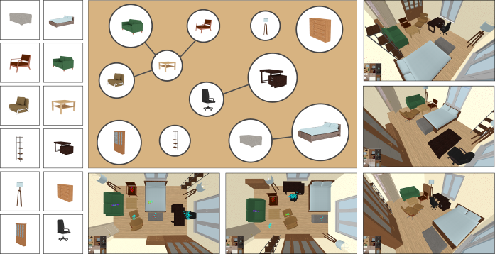
Figure 1: Given a list of objects (Left), we decompose them into disjoint groups (Top-Middle) with coherence for each individual group and freedom among groups. By incorporating discrete templates as priors to guide syntheses, our method generates various plausible layouts in seconds.

Second, due to innumerable strategies of arrangement, it is hard to exhaustively list all possible spatial relations among objects [5, 6, 31, 45, 22] or to mathematically formulate unified and accurate models for them [13, 44, 40, 41]. For example, Chang et al. [5] dictate a specific set of possible relations such as “support”, “right”, “front”, etc, which fundamentally limit the variety of possibly synthesized scenes. To model relations with multiple patterns, a common approach is to fit observed layouts with models. However, “fitting models” could potentially introduce noises and be influenced by noises, especially when the underlying patterns do not satisfy with the assumptions of models, e.g., a commonly used Gaussian mixture model (GMM). Figure 3 shows a failure case of sampling a relative position and an orientation from a GMM of a chair w.r.t a table. We argue that when the observed data is of sufficient size, the correct case inside observations or samples for fitting already offers exact layout strategies with varieties.

To address the above difficulties, in this paper, we propose a method to measure the strength of spatial relations between objects by utilizing tests for complete spatial randomness (CSR) [9]. A test for CSR (Section 4) describes how likely a set of events are generated w.r.t a homogeneous Poisson process. Intuitively, it measures how obvious certain patterns exist in a set of points. Therefore, objects with high measurements tend to be grouped and arranged together. Objects that fail to pass tests for CSR are ignored, even if they have high co-occurrence.

Furthermore, we present an approach for extracting discrete representation of various shapes of layout strategies, incorporating density peak clustering [34]. Finally, we present a framework for automatically synthesizing various arrangements of given objects w.r.t an input room geometry, by partitioning input objects into disjoint groups according to the extracted priors, followed by optimization based on the Hausdorff metric to cope with discrete priors. The entire process can be done in seconds.

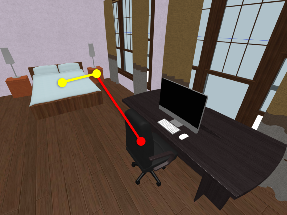
(a) A bedroom.

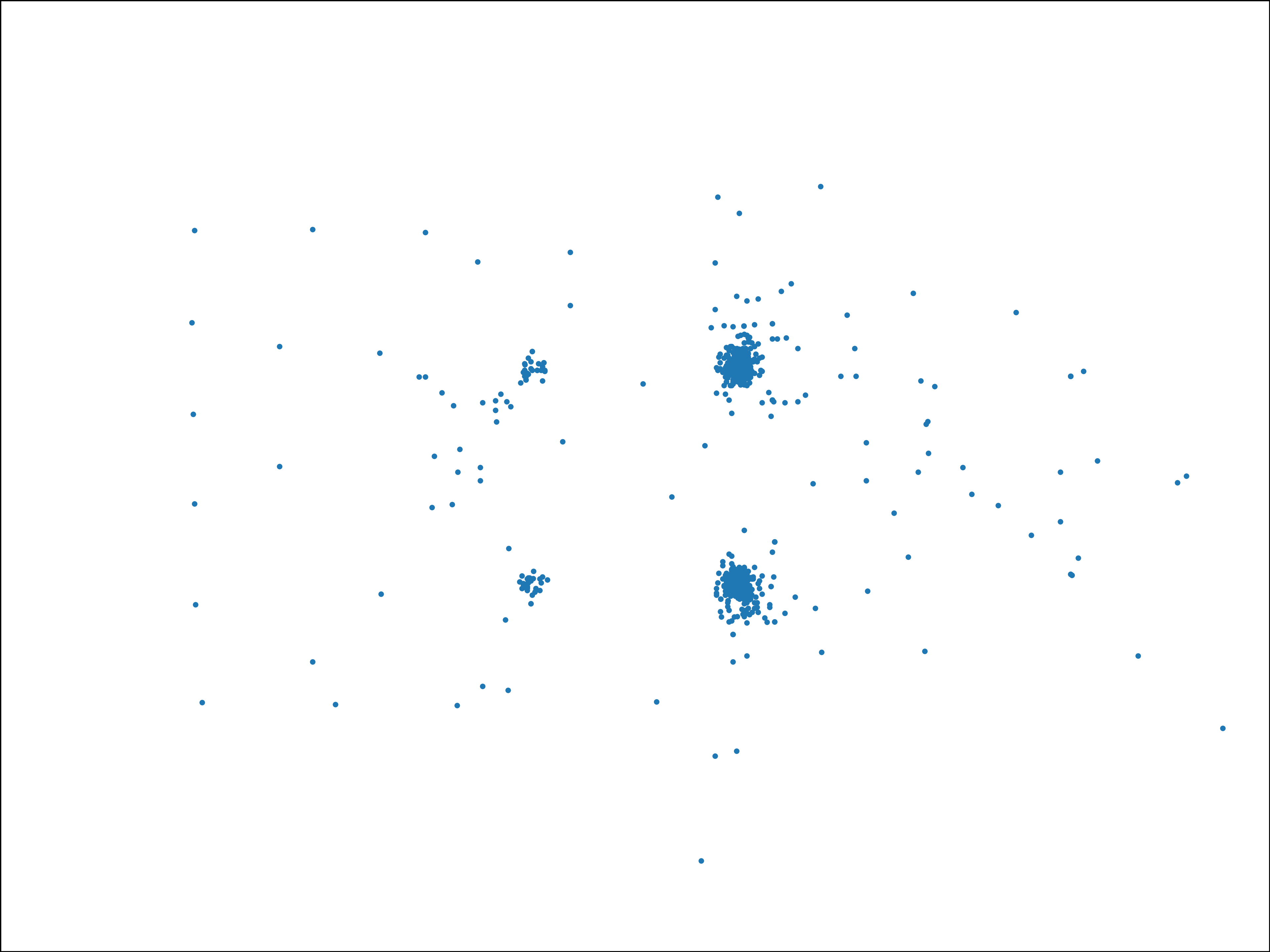
(b) A stand & a bed.

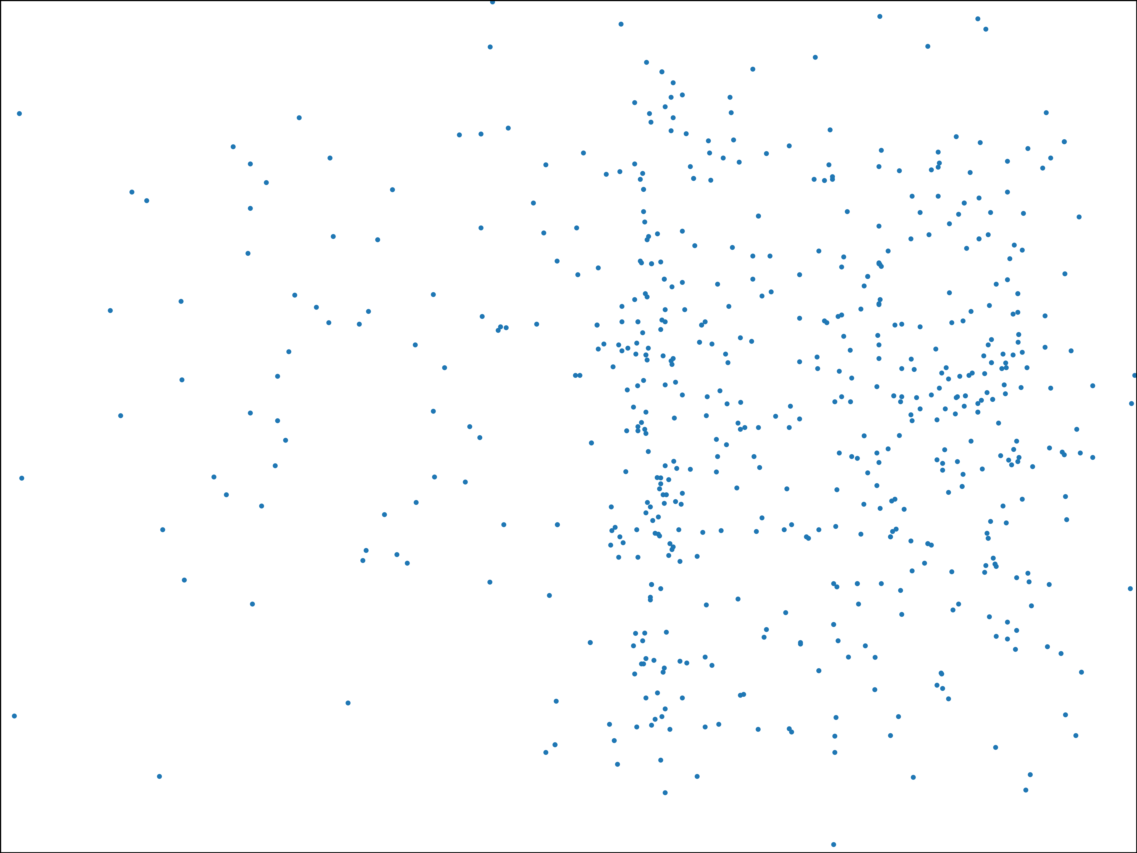
(c) A stand & a chair.

Figure 2: Illustrating the problems of co-occurrence. With similar co-occurrence, two relative positions of two pairs of objects are shown in 2(a). In 2(b), the double bed and the stand are obviously spatial related, while the stand and the chair are distributed randomly.

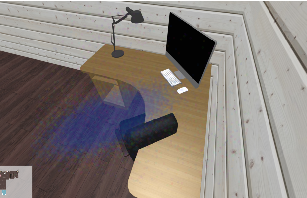
(a) GMM.

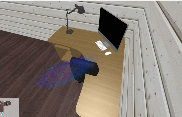
(b) GMM fits ours.

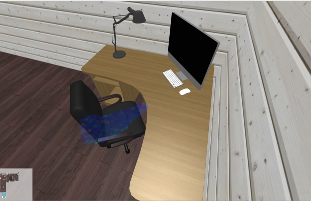
(c) Ours.

Figure 3: Inherent problems of fitting models. Fitting raw data (Left) suffers with noises. GMM fitting our denoised data (Middle) gives a blurred pattern. Ours (Right) successfully places the chair at the right place in a correct orientation.

In sum our work makes the following contributions:

1. We first incorporate tests for complete spatial randomness to measure the strength of spatial relations between objects, which is a more powerful measurement than “co-occurrence”, allowing us to decompose a given list of objects into several disjoint groups. Therefore, unnecessary calculations are reduced whilst the plausibility is increased for indoor scene modeling.

2. We propose to use discrete and exact distributions to represent layout patterns of arbitrary shapes of objects for indoor scene configurations.

3. We introduce a fast indoor scene synthesis framework, which is able to generate diverse arrangements in seconds.

2 Related Works

3D Indoor Scene Synthesis aims at generating appropriate layouts of furniture objects for rooms. Various solutions considering different input settings and tasks have been proposed. For example, [3, 7, 14, 37] generate room layouts based on RGB-D images or 3D scans. Human language [6, 5, 30] and hand-drawn sketches [44] have also been explored as additional inputs to guide scene synthesis. [41, 33, 29] iteratively infer the next objects to rooms. A full review of existing works on indoor scene synthesis is beyond the scope of this paper. Please refer to an insightful survey in [48].

As discussed in Section 1, representations of layout strategies play an important role in 3D indoor scene synthesis. To encode prior knowledge, [45, 31, 42] attempt to quantify interior design rules. The emerging availability of 3D indoor scene datasets enables various data-driven approaches. For example, [40, 6] model spatial relations between objects using semantics such as “left”, “right”, “front”, etc. Gaussian mixture models (GMMs) are adopted by [13, 44, 19] to fit observed distributions of objects. Graph structures are constructed by [32, 15]. As surveyed in [48], [46, 25] model contexts for objects, e.g., average orientations and distances between objects, orientations w.r.t the nearest walls, etc. However, despite the variety of representations, the underlying metrics are still confined to co-occurrence, model fitting or even intuitive semantics, e.g., probabilities of edges are calculated by co-existing frequencies [13, 32].

Our task partially resembles [46] and [42], but takes an automatic approach to extract constraints from existing layouts. We are also inspired by the works of [13] and [43]. However, the former requires exemplar scenes as input, while the latter focuses on re-arrangement of existing scenes. In contrast, we aim to learn general patterns for pairs of objects from existing layout examples for scene synthesis.

Tests for Complete Spatial Randomness (CSR) is a classical topic [11]. Given a series of points distributed on a plane, a test for CSR is typically used to answer how likely the points are placed randomly. Formally, it describes how likely a set of events are generated w.r.t a homogeneous Poisson process (planar Poisson process). Previously, most applications of CSR are confined to ecology [17], e.g., to investigate whether or not a set of observed plants are located with patterns. Rosin [35] is probably the first to bring the concept of CSR into computer vision to handle the problem of how to detect white noises inside images. Typical methods of tests for CSR include using Diggle’s function [9, 20], distance-based methods [11], etc. In this paper, we follow [2] to test CSR by means of angles (Section 4).

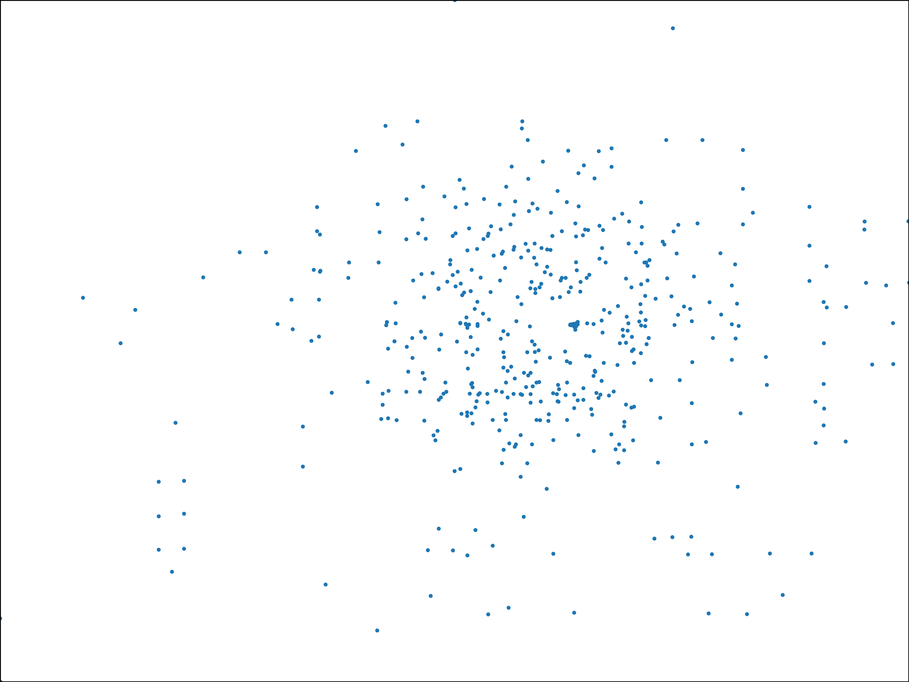
(a) $d^{wa,ct}=1.12$.

(b) $d^{dt,ch}=2.03$.

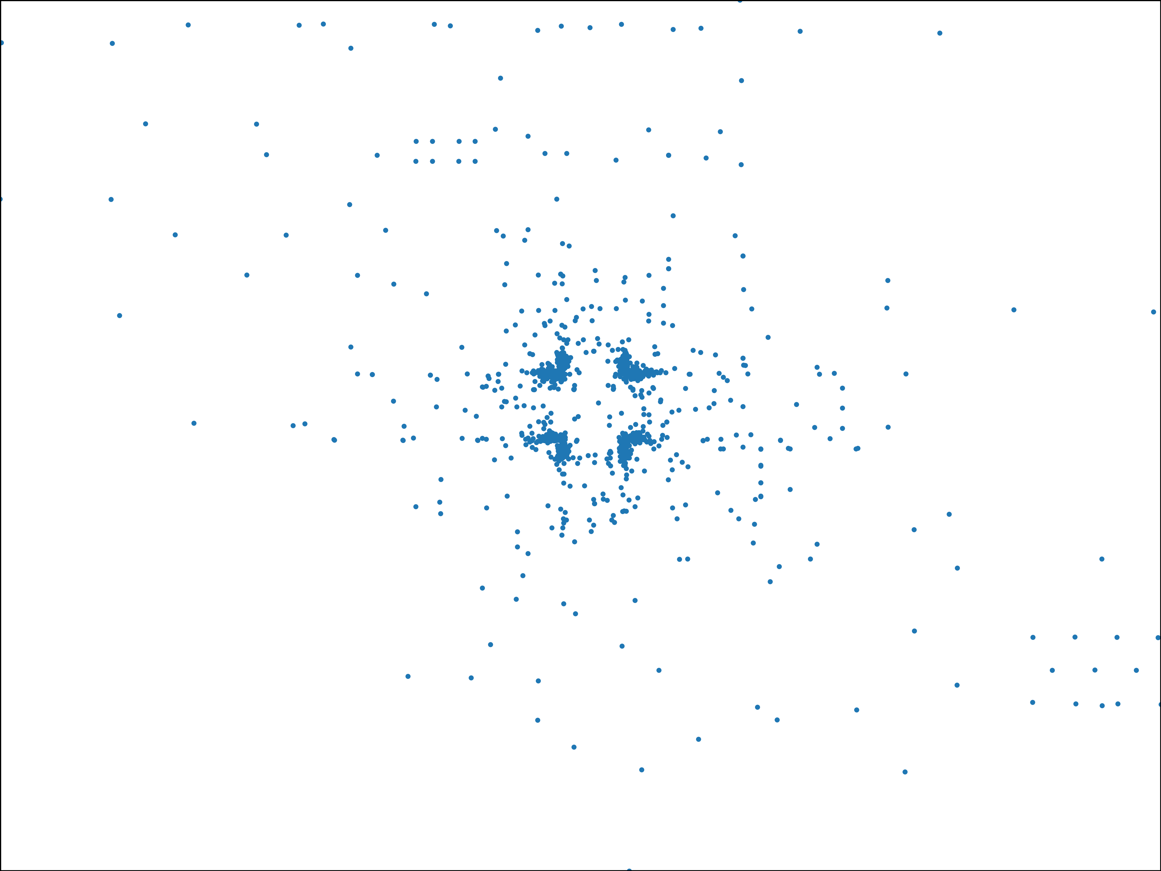
(c) $d^{be,ni}=2.47$.

Figure 4: Several results of tests for CSR. 4(a) plots relative positions between a wardrobe cabinet and a coffee table, 4(b) plots relative positions between a dinning table and a chair, and 4(c) plots relative positions between a bed and a nightstand.

3 Overview

Our pipeline is split into an offline stage and an online stage. In the offline stage, we first learn the spatial strength graph $G_{ss}$ indicating how objects are spatially related with each other (section 4). This is more powerful than counting co-occurrence. We also extract versatile patterns of layout strategies as discrete “templates” and reduce noises within datasets such as SUNCG [38] (Section 5). Given learned priors, an empty room, and a set of user-specified objects, during the online stage, our method first groups spatially coherent objects into groups (e.g., a bed and two night stand, as illustrated in Figure 9(b)). Next, we do an instant arrangement for each group by heuristically using learned templates. Finally, we adjust the overall layout by optimizing a consistent loss function (Section 6).

In formal, the offline input is a multigraph $G_{in}=(V_{in},E_{in})$, which is a direct mathematical representation of original datasets, i.e., each vertex corresponds to an objects and each edge corresponds to a displacement between two objects. A vertex $v_{in}^{i}\in V_{in}$ contains a set of attributes $\{(d_{wall}^{i,\omega},\theta_{wall}^{i,\omega},t_{wall}^{i,\omega})|\omega=1,2,3\dots,\Omega\}$, i.e., the row values of distances, orientations and translations w.r.t its nearest walls.

Centering an object $o_{i}$, the $k$-th edge $e_{in}^{i,j,k}\in E_{in}$ from $v_{in}^{i}$ to $v_{in}^{j}$ is valued by a quadruple $(p_{x}^{i,j,k},p_{y}^{i,j,k},p_{z}^{i,j,k},p_{\theta}^{i,j,k})$ representing the $k$-th relative translation and orientation of $o_{j}$ w.r.t $o_{i}$. And we leverage $E_{in}^{i,j}$ to indicate the set of edges formed from $v_{in}^{i}$ to $v_{in}^{j}$, where $v_{in}^{i}$ is the corresponding vertex in $V_{in}$ of object $o_{i}$.

We construct $G_{in}$ with 2266 vertices, over 2 million edges from more than 520,000 rooms in SUNCG dataset, and measure their strength of spatial relations in Section 4 and extract layout priors in Section 5.

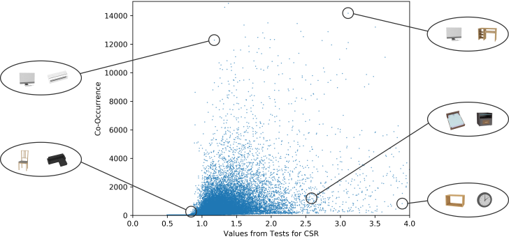
(a)

(b)

Figure 5: 5(a) plots the CSR value and co-occurrence of every pair of objects. Two objects might co-occur in many rooms, while the strength of their spatial relation could be low, vice versa. For example, the bed and the nightstand do have patterns of each other despite their low co-occurrence. 5(b) plots how tests for CSR are able to retain relations which are mistakenly removed by co-occurrence with increasing thresholds set for co-occurrence.

4 Spatial Strength Graph

Before actually extracting a template from datasets for each pair of objects, a question naturally arises: do we require templates for all pairs? As shown in Figure 2, two objects could have very messy layout strategies, with transformations between them rather independent of each other, even though they might have high co-occurrence. This motivates us to learn a spatial strength graph (SSG) so that a multitude of pairs of objects that have low relations of spatial strength are ignored when arranging rooms. This will help us synthesize more plausible scenes but also accelerate the synthesis process.

Formally, an SSG is a weighted graph defined as $G_{ss}=(V_{ss},E_{ss})$, where $G_{ss}$ denotes an entire graph, with $V_{ss}=V_{in}$ representing all objects in the dataset, and $E_{ss}$ is the edges with weight to encode spatial strength between objects. We measure the weights of $E_{ss}$ by equation 1 that is “d-value” [2] within the domain of tests for complete spatial randomness (CSR) [9]:

$$d=\sqrt{m}\sup|F_{c}(\theta)-F_{e}(\theta)|.$$ (1)

$F_{c}$ and $F_{e}$ are respectively cumulative distribution function (CDF) and empirical distribution function (EDF) w.r.t angle $\theta$, which is subject to uniform distribution [2]. $m$ is the number of points formulating the $F_{e}$. For each pair of objects $o_{i}$ and $o_{j}$, the weights $E_{ss}^{i,j}$ is set to $d^{i,j}$ subject to random samples from $E_{in}^{i,j}$ in a ratio of 10%, as suggested in [2] and [10]. As shown in figure 4(a), a wardrobe and a coffee table are spatilly independent, so their d-value is low. Although considerable noises exist in figure 4(b), d-value of a dinning table and a chair is still reasonablly high. Finally, figure 4(c) shows clear patterns between a bed and a nightstand.

Figure 5 suggests the differences between tests for CSR and co-occurrences. In figure 5(a), we plot two measurements for all pairs of objects, where pairs including an air-conditioner typically co-occur frequently but air-conditioners are placed independently to most of other objects. Figure 5(b) illustrates how tests for CSR are able to retain relations mistakenly removed by co-occurrences,

5 Prior Extraction

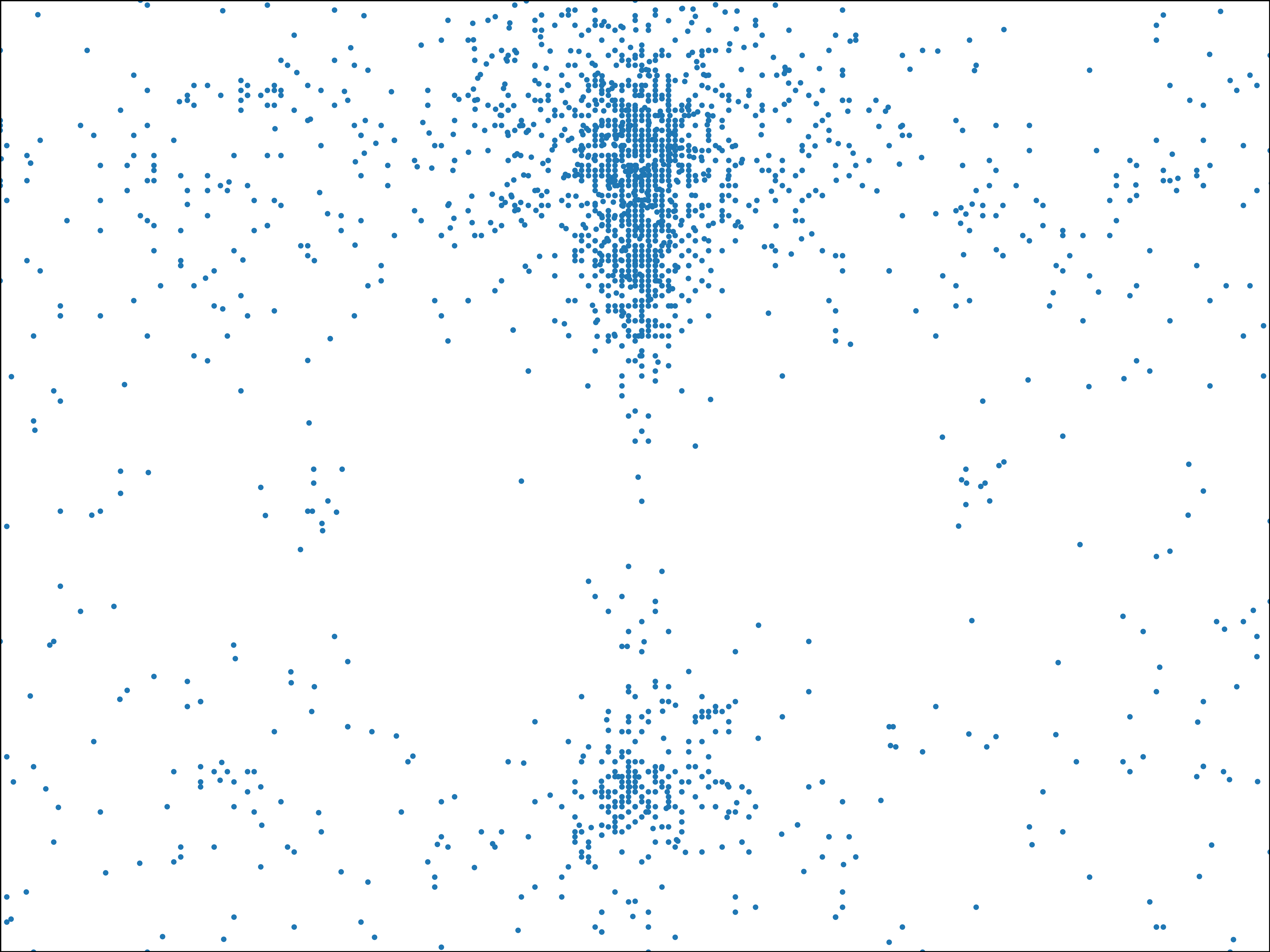
(a) Input.

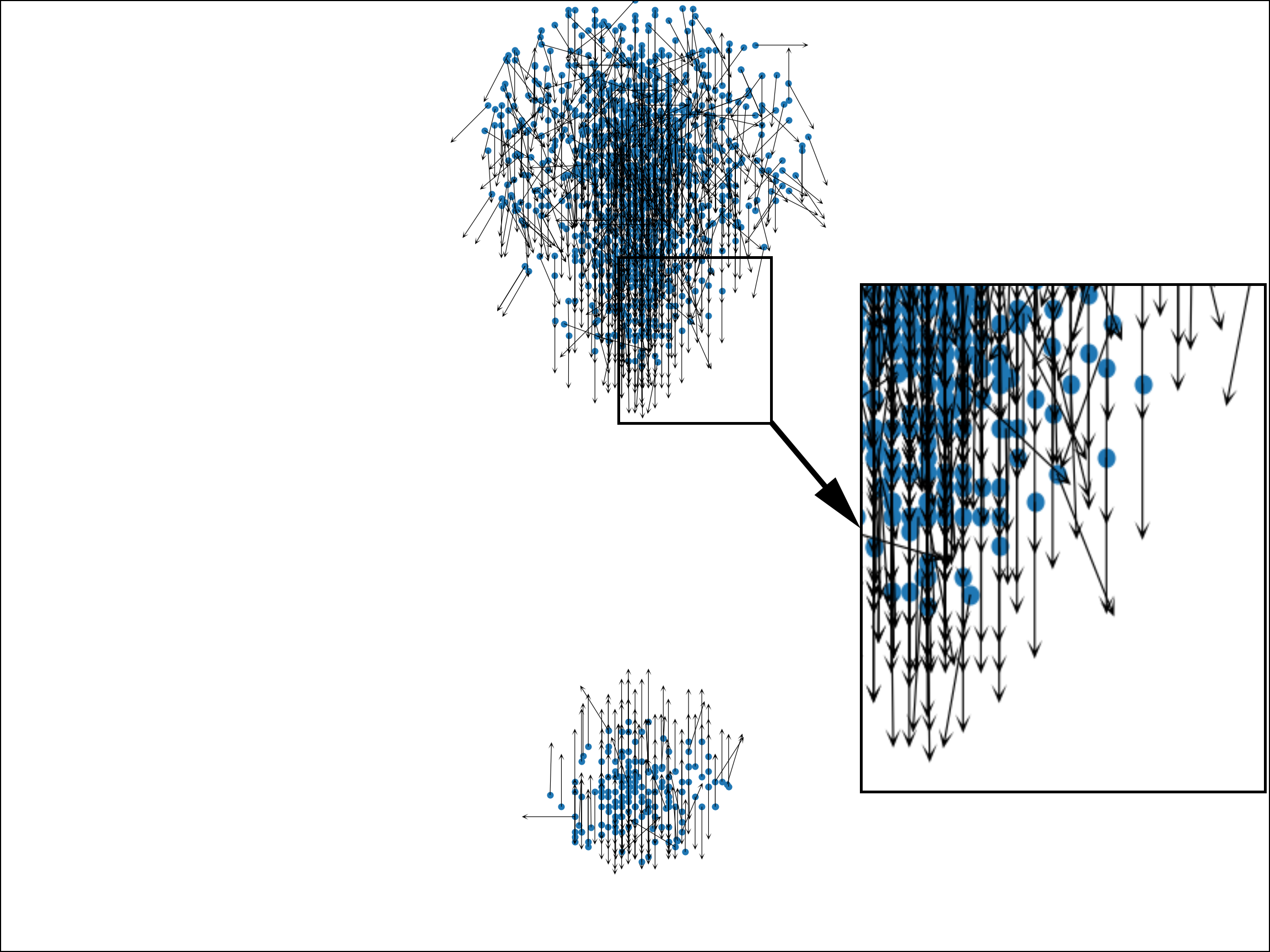
(b) De-noised.

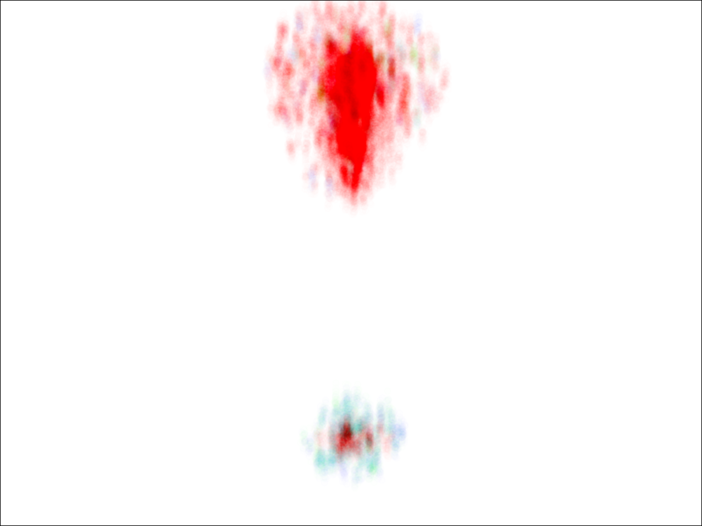
(c) Fitted.

Figure 6: The overall process of prior extraction. 6(a) is the input with considerable noises. 6(b) de-noises the input, which is readily to use in our framework, while 6(c) depicts the further generalization of our templates into fitted models which are applicable for other frameworks such as MCMC

Patterns are priors suggesting how we arrange objects in real life layouts. Figure 6(c) shows a pattern of a laptop w.r.t an office chair. Since relative translations are incorporated, patterns can inherently avoid some unreasonable situations such as collisions. However, it is obvious that we cannot set a unified model for all patterns, since the patterns can have arbitrary shapes. To extract arbitrary-shaped patterns in discrete representations, we adopt the approach in [34], which clusters points according to $\rho$ (equation 2) and $\delta$ (equation 3), where the indicating function $I_{\{d\leq d_{c}\}}$ returns $1$ if $d\leq d_{c}$ and $0$ otherwise.

$$\rho_{k} =\sum_{k^{\prime}}I_{\{d\leq d_{c}\}}(d_{k,k^{\prime}}),d_{c}=d_{(\eta K^{2})},$$ (2)

$$\delta_{k} =\min_{j\mathrel{\mathop{\mathchar 58\relax}}\rho_{k}<\rho_{k^{\prime}}}(d_{k,k^{\prime}}).$$ (3)

Given a set of edges $E^{i,j}_{in}$ from $v^{i}_{in}$ to $v^{j}_{in}$ in $G_{in}$ as shown in Figure 6(a), we first calculate pairwise Euclidean distances between them using translations. For each edge $e^{i,j,k}_{in}$, a $\rho_{k}$ is counted as the number of other edges with distances less than $d_{c}$ to it. Taking $K$ points, $d_{c}$ is the $\eta K^{2}$- greatest value among all pairwise distances with $\eta=0.015$ as suggested by [34]. $\delta_{k}$ represents the minimal distance from a set of $e^{i,j,k^{\prime}}$ with higher $\rho_{k^{\prime}}$ than $\rho_{k}$. As a result, despite arbitrary shapes, merely edges with high $\rho_{k}$ belong to a potential pattern, and each edge with high $\rho_{k}$ and high $\delta{k}$ indexes to a potential pattern, which is analogous to a cluster center in [34]. In contrast, noises tend to have high values of $\delta$ while their local density is distinctly low. As a result, we reduce noises and highlight patterns $E^{i,j}_{p}$, as illustrated in figure 6(b). The rest of accurate patterns form a discrete templates $E_{p}^{i,j}$ are already fully usable to our framework. To incorporate our model in previous works, e.g., MCMC, our priors can be easily fitted to distributions such as using non-parametric kernel density estimation based on Gaussian kernels, as shown in Figures 6(c) and 8.

We also perform similar prior extraction tasks for individual objects with regard to their orientations and distances to the nearest walls where $d_{k,k^{\prime}}$ becomes differences of scalars. In doing so, we keep the values $t_{w},\theta_{w}$ with both high values of $\rho$ and $\delta$ to index the pattern. Then we formulate the translation and rotation priors of walls into both multinomial distribution, and assign them to their corresponding vertices in $G_{in}$.

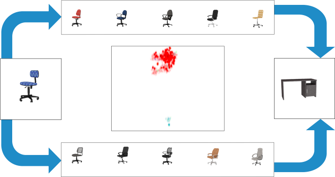
Figure 7: Assigning existing templates to new objects of similar geometry. Given a previously unseen office chair (Left), we achieve the layout strategy of it w.r.t the desk (Right) by merging templates of objects geometrically similar to the chair (Middle).

Next, we further generalize our templates to make them reusable and extensible. We observed that objects with same semantics and similar geometries share layout strategies. As shown in Figure 7, given a new object without the corresponding priors extracted from our datasets, we find its similar models by comparing 3D shapes of models using [21], which uses $s_{shed}^{k}$ to measure the degree of similarity. We select the top-$K$ results $\{(o_{k},s_{shed}^{k})|s_{shed}^{K}=\beta,k=1,2,3,\dots,K\}$ and take the union of the $K$ templates as the template for the new object, where $\beta$ is chosen as $0.1$ according to our experiments.

Figure 8 shows some results of Learnt priors. Similar to the visualization of dense optical flows [12], we apply the system of hue, saturation and value (HSV) to represent orientations, where angles are normalized within $(0,2\pi)$ as hue, probability densities are represented as saturation, and values are all set to $1$. Since height differences for most objects do not vary significantly, we plot the three channels $(p_{x}^{i,j,k},p_{z}^{i,j,k},p_{\theta}^{i,j,k})$ to make it more intuitive.

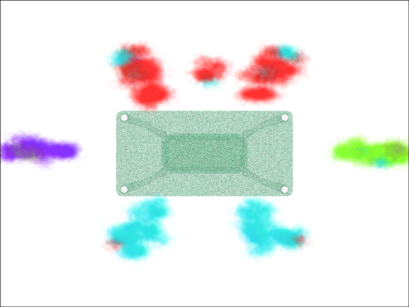
(a) CoffeeTable-Chair

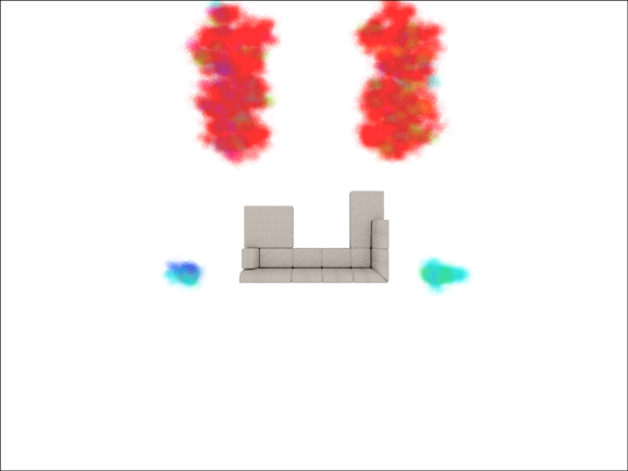
(b) Sofa-Loudspeaker

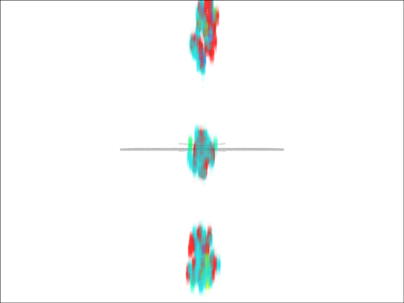
(c) TV-CoffeeTable

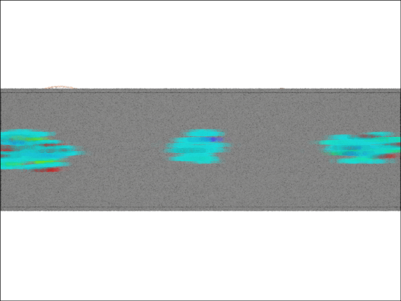
(d) TVStand-PlayStation

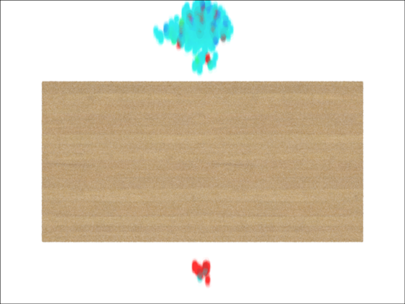
(e) Desk-OfficeChair

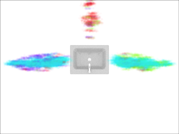
(f) Sink-Toilet

Figure 8: Several results of learnt priors.

6 Scene Synthesis

In this section, we incorporate the learnt SSG and priors to synthesize room layouts. A synthesis process typically includes two steps: a heuristic arrangement, followed by an optimization. Given a set of input objects $\hat{O}$, we first decompose them into several groups according to the SSG, and arrange objects within each group, where relative transformations are immediately indexed by the templates. Finally, we apply a global optimization to satisfy layout strategies of objects in $\hat{O}$.

6.1 Heuristic Layouts with Formulated Groups

We first construct an unweighted graph described by an adjacency matrix $M_{adj}$, whose vertices correspond to input objects $\hat{O}$. Entries of $M_{adj}$ are determined by $G_{ss}$ in Section 4. More specifically, if $d^{u,v}\geq\epsilon$, then we set $M_{adj}^{u,v}=1$, where $\epsilon$ typically equals to $1.628$ as suggested in [2]. After achieving $M_{adj}$, we iteratively construct disjoint groups $g\in Gr$ of objects by finding connected components of the graph represented by $M_{adj}$. Figure 9 shows examples of resulting groups. It is common to see a group containing only one object, such as wardrobe, cabinet or shelf, because their placement usually does not require considering other objects, Such single-object groups greatly ease the following optimization process.

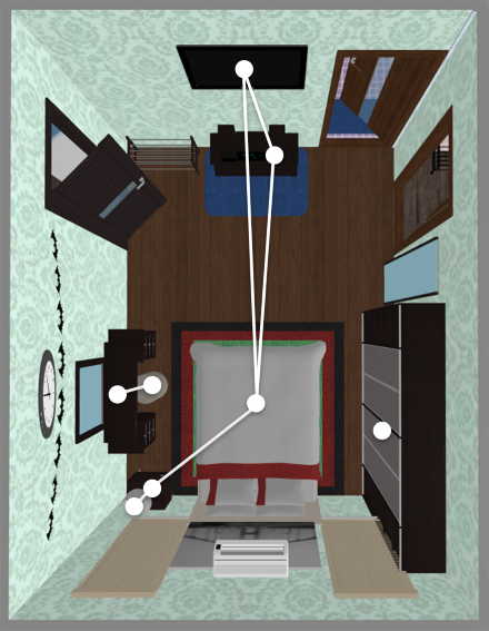
(a) Marked relations.

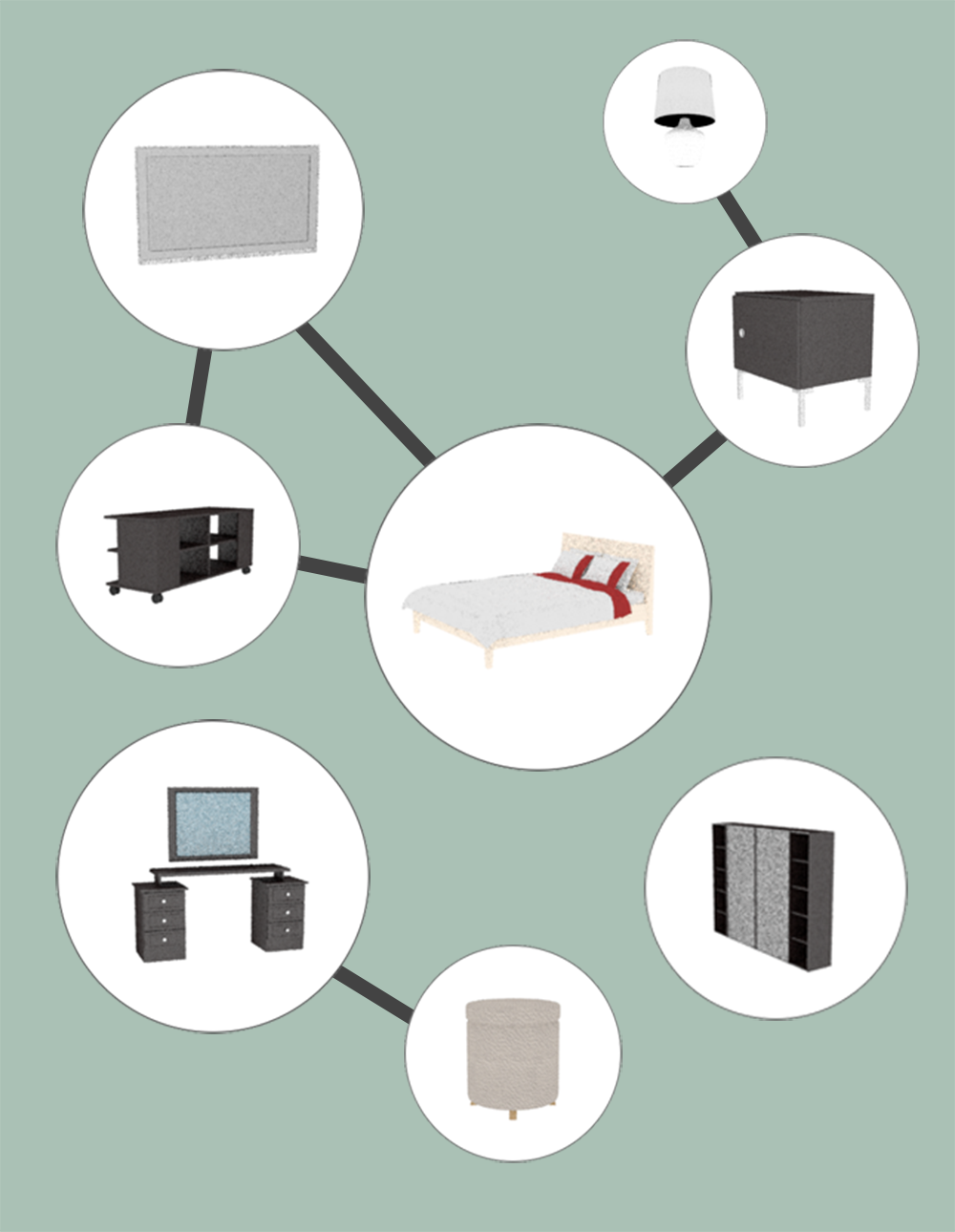
(b) Disjoint graphs.

Figure 9: Formulating functionally coherent groups of objects using tests for CSR.

Based on a given room shape, partitioned groups, and learnt templates, we then generate proposals for pending scenes, i.e., objects are immediately placed and oriented w.r.t their groups and walls. For each group $g\in Gr$, layouts of $g$ are heuristically generated by sampling a posterior probability distribution $\Psi_{G|E_{p}}(g)$ expressed in Equation 4, given templates $E_{p}$ (Section 5).

$$\Psi_{G|E_{p}}(g) =\frac{\alpha(g)\cdot\Phi_{E_{p}|G=g}(E^{\mu}_{p})}{\int\alpha(g)\cdot\Phi_{E_{p}|G=g}(E^{\mu}_{p})dg},$$ (4)

$$=\frac{\alpha(g)\cdot\sum_{\mu}\prod_{\tau\in g}\phi_{E_{p}^{\mu}|T=\tau}(E_{p}^{\mu,t},\tau^{\mu})}{\int\alpha(g)\cdot\Phi_{E_{p}|G=g}(E^{\mu}_{p})dg},$$ (5)

$\alpha(g)$ denotes the probability of each object $\tau\in g$ being the dominant object $\tau^{\mu}$ in $g$. Let $deg(\tau)$ denote the degree of $\tau$ w.r.t $M_{adj}$, which is the number of objects connected with it according to the test for CSR (Section 4), and $dmax=\max_{\tau\in g}deg(\tau)$. The likelihood $\phi_{E_{p}^{\mu}|T=\tau}(\cdot)$ is a multinomial distribution formed by the given template $E_{p}^{\mu,t}$ of $\tau$ w.r.t $\tau^{\mu}$, while it is equal to a constant when $\tau=\tau^{\mu}$.

$$\alpha(g)=\begin{cases}\frac{1}{|\{\tau|\tau\in g,deg(\tau)=dmax\}|}&,\text{ if }deg(\tau^{\mu})=dmax\\ 0&,\text{ otherwise}\end{cases},$$ (6)

When sampling $\Psi_{G|\Theta=\hat{O}}$, we first randomly decide $\tau^{\mu}$ of $g$. Equation 5 implies that $\{\phi_{E_{p}^{\mu}|T=\tau}(\cdot)|\tau\in g\}$ are independent to each other, so transformations of objects are sampled according to their own templates, respectively. In practice, if an object has a relatively low d-value to $\tau^{\mu}$, we further decompose the group and assign a new dominant object to it. In some cases, this heuristic strategy could sample a sufficiently plausible layout even without a further optimization. However, the heuristic strategy may still results in unreasonable conditions such as collision between groups, objects out of room boundaries, etc. Next we show how we adjust objects so that a plausible layout of objects is eventually presented.

6.2 Template Matching

Equation 7 mathematically formalizes template matching, where we are trying to minimize the summation of Hausdorff distances $d_{H}$ between all objects w.r.t their templates. $X^{i}$ indexes the transformation of object $o^{i}$ and $E_{p}$ is a set of sampled transformations in Section 5.

$$X^{*} =\mathop{\arg\min}_{X}L(X,E_{p})$$ (7)

$$=\mathop{\arg\min}_{X}\sum_{i,j}M_{adj}^{i,j}d_{H}(X^{i},E_{p}^{i,j})+Col(X,r),$$ (8)

$d_{H}$ is Hausdorff metric between an element to a set derived by the distance function $d_{h}$ under the space of translation and rotation. The reason for assembling Hausdorff distance is that it directly tackles samples instead of distributions. As illustrated, it is unlikely to mathematically express a unified distribution to model arbitrary layout patterns. In contrast, if we could extract samples of arbitrary shape, Hausdorff metric enables pipelines to skip model fitting and to optimize directly using refined samples.

$$d_{H}(x,S)=\min_{v\in S}d_{h}(x,s),$$ (9)

$$d_{h}(x,s) =\mathinner{\!\left\lVert x_{p}-v_{p}\right\rVert}+\exp(ori(x_{\theta},v_{\theta})),$$ (10)

$$ori(\theta,\theta^{\prime}) =\min(2\pi-\mathinner{\!\left\lvert\theta-\theta^{\prime}\right\rvert},\mathinner{\!\left\lvert\theta-\theta^{\prime}\right\rvert}),$$ (11)

Equation 12 represents the artifacts among objects and between objects and walls, where $p(\chi,k)$ returns the $k$-th rotated point position of the bounding box or the shape of $\chi$. Ideally, if there is no collision and no object out of boundary, $Col(X,r)$ should equal to $0$.

$$Col(X,r) =Col_{wall}(X,r)+Col_{obj}(X)$$

$$=\sum_{i,k}\prod_{r}tR(p(X_{i},k),p(R,r),p(R,r+1))$$

$$+\sum_{i,k,j}\prod_{l}tL(p(X_{i},k),p(X_{j},l),p(X_{j},l+1))$$ (12)

$Col_{wall}$ measures whether or not objects are out of walls, whilst $Col_{obj}$ calculates overlaps among objects. Truncated by $tR(\cdot)$ and $tL(\cdot)$, $\gamma(\cdot)$ represents the “to-left” test of computational geometry [8], such as the utilization in [18]. In addition to given objects, we place extra virtual objects as doors and windows with fixed transformations to avoid blocking them.

$$tR(p_{1},p_{2},p_{3}) =\max(-\gamma(p_{1},p_{2},p_{3}),0)$$ (13)

$$tL(p_{1},p_{2},p_{3}) =\max(\gamma(p_{1},p_{2},p_{3}),0)$$ (14)

Since the underlying metrics are factorized as quadratic terms, we optimize equation 9 utilizing Position-Based Dynamics (PBD) [4], which is also detailed in [42]. Incorporating heuristic approaches, syntheses require $10$ iterations to converge on average after heuristic attempts.

7 Experiments

7.1 Tests for CSR

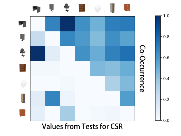
Figure 10: A comparison between values from tests for CSR and co-occurrence.

Figure 10 shows the comparison between using co-occurrence and using tests for CSR to measure the strengths of relations between objects. The results is normalized due to different scales. The upper triangular part depicts co-occurrence and the lower fills results from tests for CSR, which alleviates the unreasonableness caused by co-occurrence. The shelf is weakly related to the computer spatially, but co-occurrence suggests a strong relation.

It is obvious that placing the gray desk is independent of arranging the brown shelf, but they have a high frequency of co-existing in different rooms of various types, which potentially influences overall performances. Applying tests for CSR for them, the pair is decoupled spatially. The same is true of objects preferring independent layout with most of the others, such as the white dryer, the wardrobe and the brown stand.

7.2 Prior Sampling

Figure 11 compares priors of our work with others. Since priors model layouts with high probability of being plausible between objects, we should get likely transformations by sampling them. According to experiments, both [46] and GMM fail if noises exist in datasets, so inputs to all priors are data de-noised by us (section 5). Figure 11 shows the sampled transformations of priors, given de-noised data (section 5).

Red dots denote the centred objects. The top row is priors used by [46], where they average the relative distances and orientations. We disturb their mean distance and orientations by a Gaussian kernel $\kappa\sim\mathcal{N}(0,0.1)$. The middle row is GMM used by [44, 13]. Although we further manually set appropriate thresholds for each pattern in order to reduce potential noises as well as assembling [1] to assist explorations of number of peaks, the results are still confined to elliptical shapes such as figure 11(a), or introduced outliers such as 11(b). The bottom row shows our results. Ours are capable of detecting various layout patterns without introducing outliers. For example, figure 11(c) shows two patterns (four symmetry patterns) between a sofa and a loudspeaker.

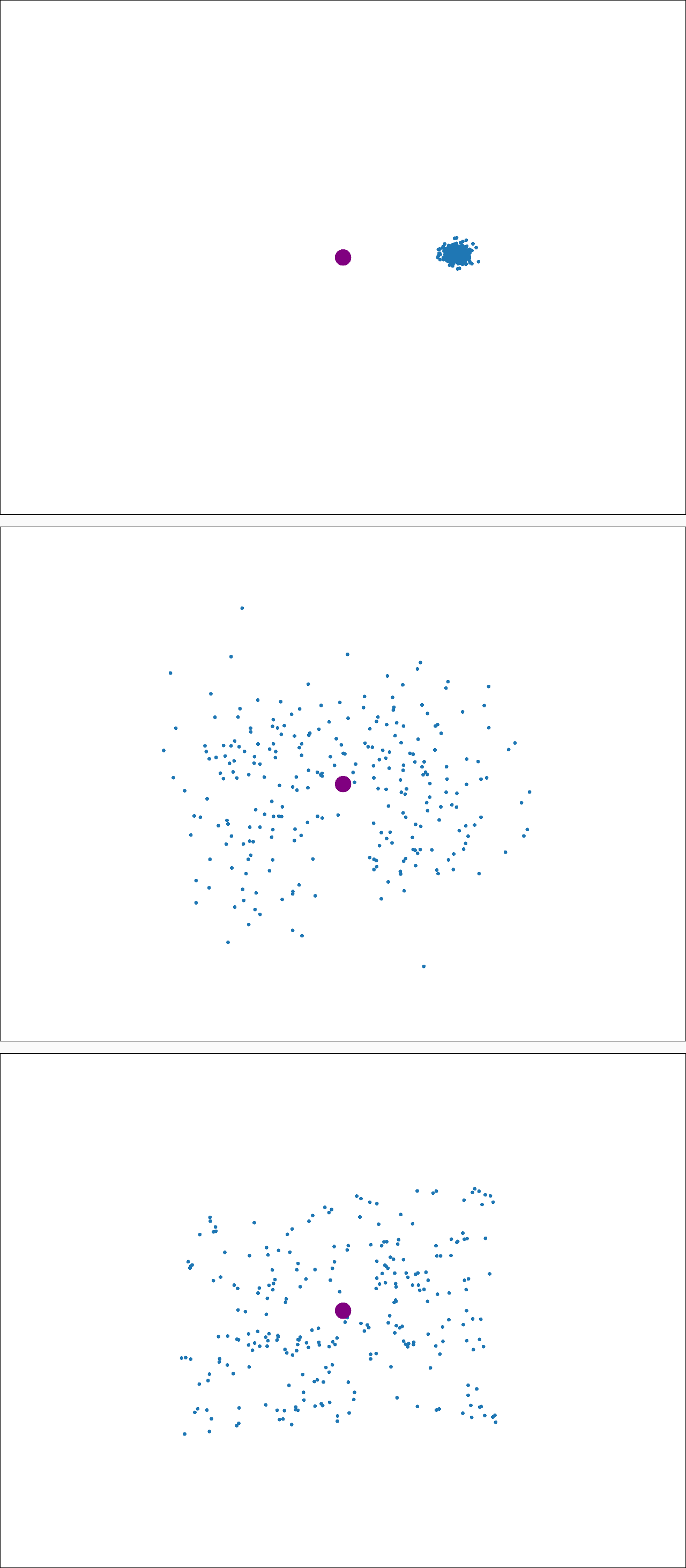
(a) DiningTable-Glass

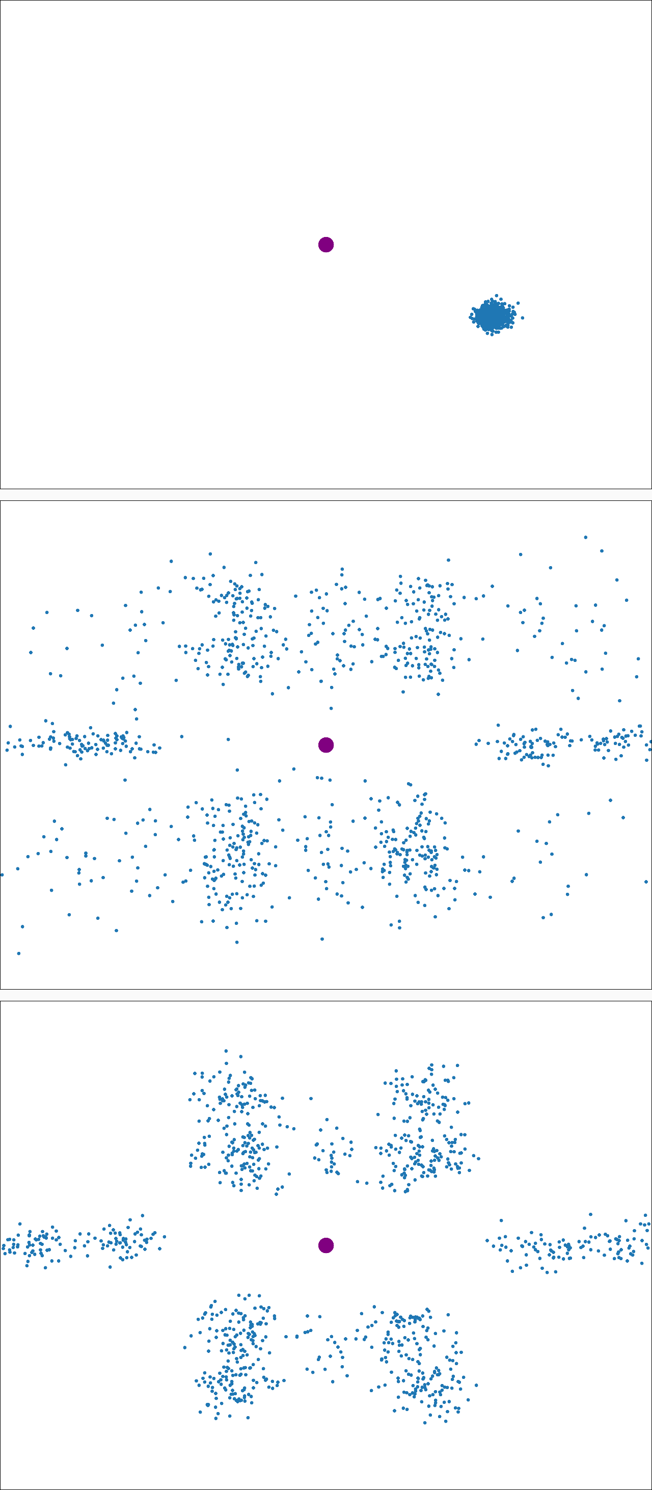
(b) LongTable-Chair

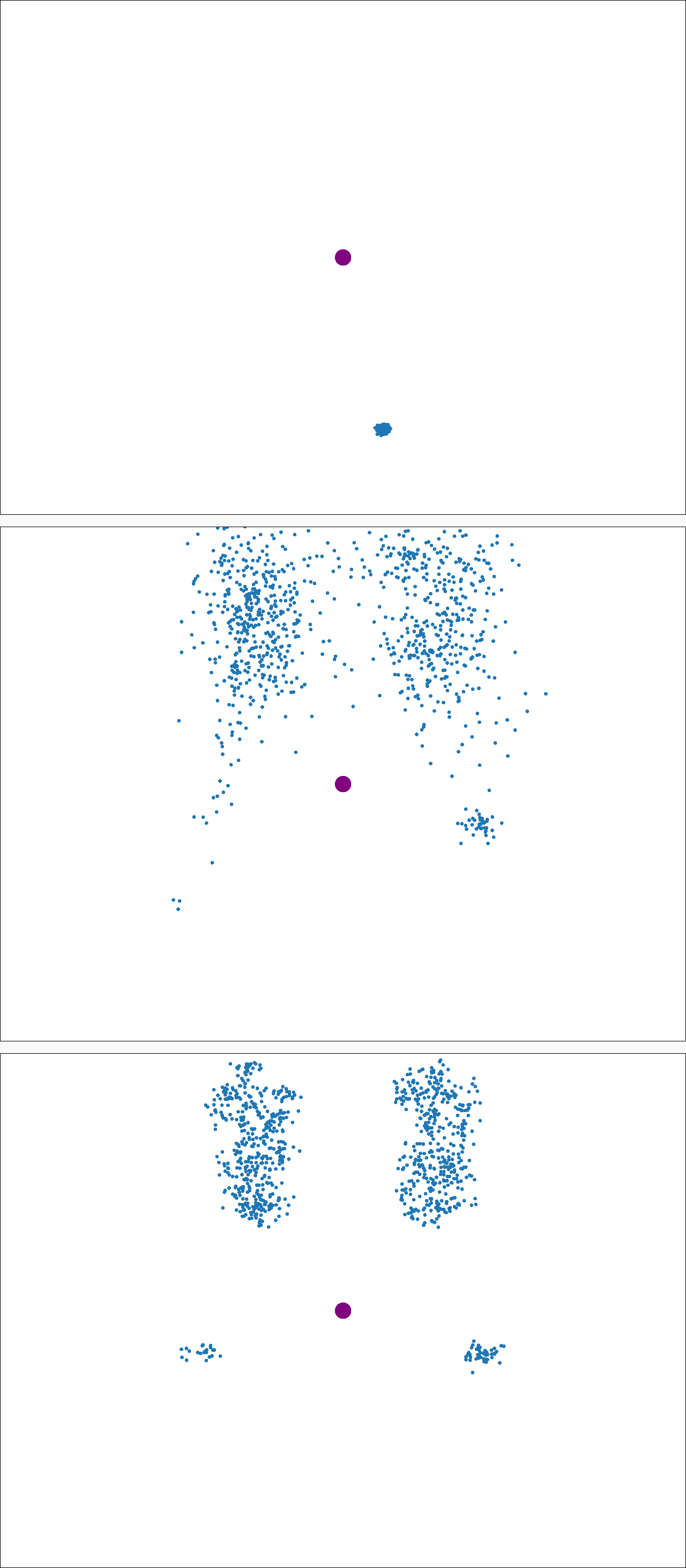
(c) Sofa-Loudspeaker

Figure 11: Sampled transformations from extracted priors between objects, where the former is centred as red dots. Top: Yu et al. [46]. Middle: Xu et al. [44], Fisher el al. [13]. Bottom: Ours.

7.3 Efficiency

Our work achieves acceleration due to the usage of PBD [4] which is verified [42] to be faster than using MCMC. However, our work is different from [42] since ours is data-driven and does not require user input to constraint for each synthesis. In this section, we conduct several experiments to show the achieved efficiency, where examples are chosen from figure 12.

We do heuristic arrangement for both [32] and [46] to speed up their work. The time costs are shown in table 1, where values with “greater-than signs” denote examples requiring more than $20000$ iterations. Experimentally, determining terminations for MCMC is hard and proposal moves are precarious. Because we judge whether or not a proposal is accepted after each iteration, resources are wasted.

Table 1: Time Consumption (sec).

	# Objects	Yu et al. [46]	Qi et al. [32]	Ours
Bedroom	9	$>$299.27s	229.76s	0.28s
Living Room	25	$>$2135.30s	1790.65s	1.88s
Bathroom	8	$>$313.54s	216.20s	0.29s
Hybrid-1	13	$>$714.60s	$>$481.35s	0.64s
Hybrid-2	35	$>$2313.38s	$>$1667.03s	2.31s
Hybrid-3	28	$>$1351.15s	1122.63s	1.24s

7.4 User Study

Table 2: User study: aesthetics.

Data	Bedroom	Living Room	Bathroom	Dinning Room	Balcony	Hall	Garage	Hybrid Room	Total
Ours	2.944	3.292	2.989	3.344	3.344	3.061	3.256	3.317	3.194
Ground Truth	2.911	3.422	3.156	3.589	3.378	2.878	3.511	3.367	3.276

Table 3: User study: evaluations of tests for CSR and co-occurrence.

Metric	Bedroom	Living Room	Bathroom	Dinning Room	Balcony	Hall	Garage	Total
Tests for CSR	93.31%	85.47%	96.67%	92.42%	86.36%	89.47%	76.17%	88.55%
Co-Occurrence	32.26%	43.81%	86.67%	45.76%	23.08%	38.46%	36.84%	43.53%

Results of our work is shown in figure 12. Formulating functional groups using CSR enables us to generate hybrid rooms. Evaluations of 3D indoor scenes are subjective, so we conduct two user studies to evaluate our method. Firstly, aesthetic measures how visually pleasing the generated scenes are, i.e., asking subjects to grade generated layouts shuffled with ground truth. Subjects grade from level-1 (poor) to level-5 (perfect). As listed in table 2, our generated results are comparable to the original layouts. Another user study is conducted to measure how tests for CSR and learnt templates satisfy intuitions of humans. We sort pairwise relations by tests for CSR and co-occurrence respectively. For each sorted list of pairs, we take templates of pairs at a fixed interval $int=120$ from the highest value. Then subjects judge whether or not the presented templates are consistent with real-life layout strategies. Tabulated in table 3, results for co-occurrence contain considerable pairs spatially independent. In total, $63$ scenes and $500$ templates are generated. We invite $97$ subjects from societies and they were merely told to grade layouts and and judge patterns.

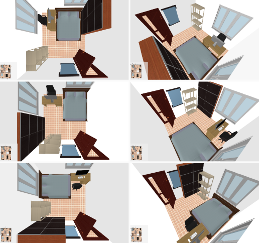
(a) Bedroom

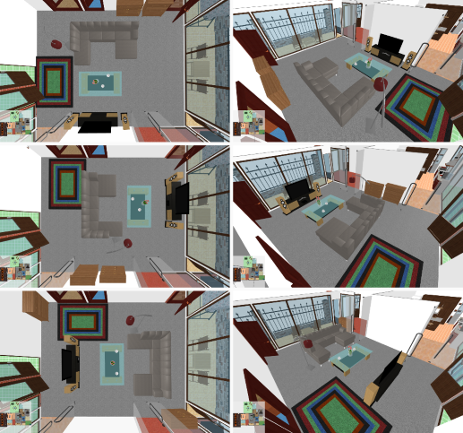
(b) Living Room

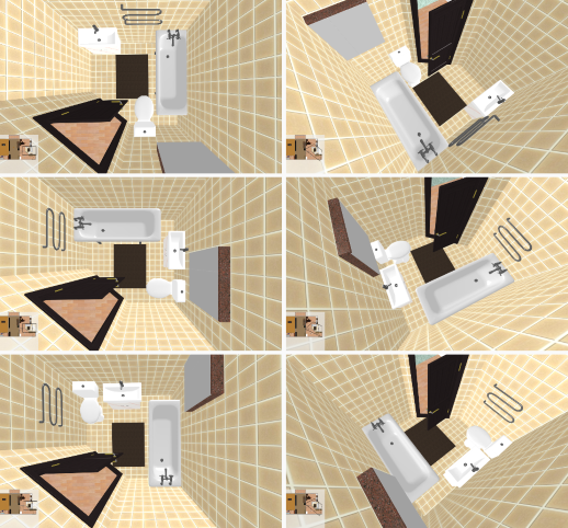
(c) Bathroom

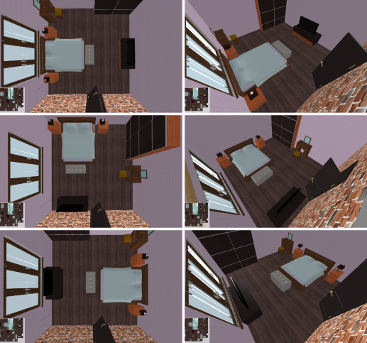
(d) Hybrid Room - 1

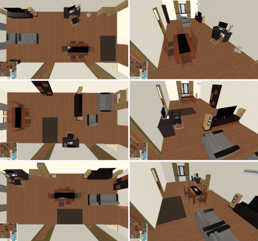
(e) Hybrid Room - 2

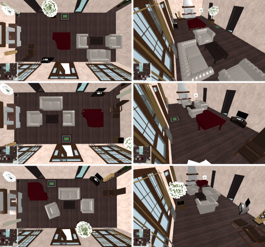
(f) Hybrid Room - 3

Figure 12: Examples of various synthesized results. Each scene is generated with three alternative layouts in top views followed by side views.

8 Conclusion

In this paper, we present a framework for 3D indoor scene synthesis based on analysis of patterns. We experimentally verify the correctness, generalization and effectiveness of it. Our framework is capable of further expansion by easily incorporating object selections such as [32, 26]. Future work includes getting finer comparisons of 3D shapes for generalizing our templates such as 3DMatch [47]. Recently, improvements for density peak clustering are also available [39, 27]. We hope the pipeline, learnt models and synthesized layouts can contribute to automatic room layouts as well as associated domains such as scene understanding [36].

References

- [1] Hirotogu Akaike. Information theory and an extension of the maximum likelihood principle. In Selected papers of hirotugu akaike, pages 199–213. Springer, 1998.
- [2] Renato Assuncao. Testing spatial randomness by means of angles. Biometrics, pages 531–537, 1994.
- [3] Armen Avetisyan, Manuel Dahnert, Angela Dai, Manolis Savva, Angel X Chang, and Matthias Nießner. Scan2cad: Learning cad model alignment in rgb-d scans. arXiv preprint arXiv:1811.11187, 2018.
- [4] Jan Bender, Matthias Müller, Miguel A Otaduy, Matthias Teschner, and Miles Macklin. A survey on position-based simulation methods in computer graphics. In Computer graphics forum, volume 33, pages 228–251. Wiley Online Library, 2014.
- [5] Angel Chang, Will Monroe, Manolis Savva, Christopher Potts, and Christopher D Manning. Text to 3d scene generation with rich lexical grounding. arXiv preprint arXiv:1505.06289, 2015.
- [6] Angel Chang, Manolis Savva, and Christopher D Manning. Learning spatial knowledge for text to 3d scene generation. In Proceedings of the 2014 Conference on Empirical Methods in Natural Language Processing (EMNLP), pages 2028–2038, 2014.
- [7] Kang Chen, Yukun Lai, Yu-Xin Wu, Ralph Robert Martin, and Shi-Min Hu. Automatic semantic modeling of indoor scenes from low-quality rgb-d data using contextual information. ACM Transactions on Graphics, 33(6), 2014.
- [8] Mark De Berg, Marc Van Kreveld, Mark Overmars, and Otfried Schwarzkopf. Computational geometry. In Computational geometry, pages 1–17. Springer, 1997.
- [9] Peter J Diggle. On parameter estimation and goodness-of-fit testing for spatial point patterns. Biometrics, pages 87–101, 1979.
- [10] Peter J Diggle, Julian Besag, and J Timothy Gleaves. Statistical analysis of spatial point patterns by means of distance methods. Biometrics, pages 659–667, 1976.
- [11] Peter J Diggle et al. Statistical analysis of spatial point patterns. Academic press, 1983.
- [12] Gunnar Farnebäck. Two-frame motion estimation based on polynomial expansion. In Scandinavian conference on Image analysis, pages 363–370. Springer, 2003.
- [13] Matthew Fisher, Daniel Ritchie, Manolis Savva, Thomas Funkhouser, and Pat Hanrahan. Example-based synthesis of 3d object arrangements. ACM Transactions on Graphics (TOG), 31(6):135, 2012.
- [14] Matthew Fisher, Manolis Savva, Yangyan Li, Pat Hanrahan, and Matthias Nießner. Activity-centric scene synthesis for functional 3d scene modeling. ACM Transactions on Graphics (TOG), 34(6):179, 2015.
- [15] Qiang Fu, Xiaowu Chen, Xiaotian Wang, Sijia Wen, Bin Zhou, and Hongbo Fu. Adaptive synthesis of indoor scenes via activity-associated object relation graphs. ACM Transactions on Graphics (TOG), 36(6):201, 2017.
- [16] Tobias Germer and Martin Schwarz. Procedural arrangement of furniture for real-time walkthroughs. In Computer Graphics Forum, volume 28, pages 2068–2078. Wiley Online Library, 2009.
- [17] Jacques Gignoux, Camille Duby, and Sébastian Barot. Comparing the performances of diggle’s tests of spatial randomness for small samples with and without edge-effect correction: application to ecological data. Biometrics, 55(1):156–164, 1999.
- [18] Ronald L. Graham. An efficient algorithm for determining the convex hull of a finite planar set. Info. Pro. Lett., 1:132–133, 1972.
- [19] Paul Henderson, Kartic Subr, and Vittorio Ferrari. Automatic generation of constrained furniture layouts. arXiv preprint arXiv:1711.10939, 2017.
- [20] LP Ho and SN Chiu. Testing the complete spatial randomness by diggle’s test without an arbitrary upper limit. Journal of Statistical Computation and Simulation, 76(07):585–591, 2006.
- [21] Yanir Kleiman, Oliver van Kaick, Olga Sorkine-Hornung, and Daniel Cohen-Or. Shed: shape edit distance for fine-grained shape similarity. ACM Transactions on Graphics (TOG), 34(6):235, 2015.
- [22] Manyi Li, Akshay Gadi Patil, Kai Xu, Siddhartha Chaudhuri, Owais Khan, Ariel Shamir, Changhe Tu, Baoquan Chen, Daniel Cohen-Or, and Hao Zhang. Grains: Generative recursive autoencoders for indoor scenes. ACM Transactions on Graphics (TOG), 38(2):12, 2019.
- [23] Wenbin Li, Sajad Saeedi, John McCormac, Ronald Clark, Dimos Tzoumanikas, Qing Ye, Yuzhong Huang, Rui Tang, and Stefan Leutenegger. Interiornet: Mega-scale multi-sensor photo-realistic indoor scenes dataset. In British Machine Vision Conference (BMVC), 2018.
- [24] Yabei Li, Junge Zhang, Yanhua Cheng, Kaiqi Huang, and Tieniu Tan. Df 2 net: Discriminative feature learning and fusion network for rgb-d indoor scene classification. In Thirty-Second AAAI Conference on Artificial Intelligence, 2018.
- [25] Yuan Liang, Fei Xu, Song-Hai Zhang, Yu-Kun Lai, and Taijiang Mu. Knowledge graph construction with structure and parameter learning for indoor scene design. Computational Visual Media, 4(2):123–137, 2018.
- [26] Yuan Liang, Song-Hai Zhang, and Ralph Robert Martin. Automatic data-driven room design generation. In International Workshop on Next Generation Computer Animation Techniques, pages 133–148. Springer, 2017.
- [27] Ruhui Liu, Weiping Huang, Zhengshun Fei, Kai Wang, and Jun Liang. Constraint-based clustering by fast search and find of density peaks. Neurocomputing, 330:223–237, 2019.
- [28] Gloria Hander Lyons. Ten Common Home Decorating Mistakes & How to Avoid Them. Blue Sage Press, 2008.
- [29] Rui Ma, Honghua Li, Changqing Zou, Zicheng Liao, Xin Tong, and Hao Zhang. Action-driven 3d indoor scene evolution. ACM Trans. Graph., 35(6):173–1, 2016.
- [30] Rui Ma, Akshay Gadi Patil, Matthew Fisher, Manyi Li, Sören Pirk, Binh-Son Hua, Sai-Kit Yeung, Xin Tong, Leonidas Guibas, and Hao Zhang. Language-driven synthesis of 3d scenes from scene databases. In SIGGRAPH Asia 2018 Technical Papers, page 212. ACM, 2018.
- [31] Paul Merrell, Eric Schkufza, Zeyang Li, Maneesh Agrawala, and Vladlen Koltun. Interactive furniture layout using interior design guidelines. In ACM transactions on graphics (TOG), volume 30, page 87. ACM, 2011.
- [32] Siyuan Qi, Yixin Zhu, Siyuan Huang, Chenfanfu Jiang, and Song-Chun Zhu. Human-centric indoor scene synthesis using stochastic grammar. In Proceedings of the IEEE Conference on Computer Vision and Pattern Recognition, pages 5899–5908, 2018.
- [33] Daniel Ritchie, Kai Wang, and Yu-an Lin. Fast and flexible indoor scene synthesis via deep convolutional generative models. In Proceedings of the IEEE Conference on Computer Vision and Pattern Recognition, pages 6182–6190, 2019.
- [34] Alex Rodriguez and Alessandro Laio. Clustering by fast search and find of density peaks. Science, 344(6191):1492–1496, 2014.
- [35] Paul Rosin. Thresholding for change detection. In Sixth International Conference on Computer Vision (IEEE Cat. No. 98CH36271), pages 274–279. IEEE, 1998.
- [36] Scott Satkin, Jason Lin, and Martial Hebert. Data-driven scene understanding from 3d models. 2012.
- [37] Tianjia Shao, Weiwei Xu, Kun Zhou, Jingdong Wang, Dongping Li, and Baining Guo. An interactive approach to semantic modeling of indoor scenes with an rgbd camera. ACM Transactions on Graphics (TOG), 31(6):136, 2012.
- [38] Shuran Song, Fisher Yu, Andy Zeng, Angel X Chang, Manolis Savva, and Thomas Funkhouser. Semantic scene completion from a single depth image. Proceedings of 30th IEEE Conference on Computer Vision and Pattern Recognition, 2017.
- [39] Bangyu Tong. Density peak clustering algorithm based on the nearest neighbor. In 3rd International Conference on Mechatronics Engineering and Information Technology (ICMEIT 2019). Atlantis Press, 2019.
- [40] Kai Wang, Yu-An Lin, Ben Weissmann, Manolis Savva, Angel X Chang, and Daniel Ritchie. Planit: Planning and instantiating indoor scenes with relation graph and spatial prior networks. ACM Transactions on Graphics (TOG), 38(4):132, 2019.
- [41] Kai Wang, Manolis Savva, Angel X Chang, and Daniel Ritchie. Deep convolutional priors for indoor scene synthesis. ACM Transactions on Graphics (TOG), 37(4):70, 2018.
- [42] Tomer Weiss, Alan Litteneker, Noah Duncan, Masaki Nakada, Chenfanfu Jiang, Lap-Fai Yu, and Demetri Terzopoulos. Fast and scalable position-based layout synthesis. arXiv preprint arXiv:1809.10526, 2018.
- [43] Hualiang Xie, Wenzhuo Xu, and Bin Wang. Reshuffle-based interior scene synthesis. In Proceedings of the 12th ACM SIGGRAPH International Conference on Virtual-Reality Continuum and Its Applications in Industry, pages 191–198. ACM, 2013.
- [44] Kun Xu, Kang Chen, Hongbo Fu, Wei-Lun Sun, and Shi-Min Hu. Sketch2scene: sketch-based co-retrieval and co-placement of 3d models. ACM Transactions on Graphics (TOG), 32(4):123, 2013.
- [45] Yi-Ting Yeh, Lingfeng Yang, Matthew Watson, Noah D Goodman, and Pat Hanrahan. Synthesizing open worlds with constraints using locally annealed reversible jump mcmc. ACM Transactions on Graphics (TOG), 31(4):56, 2012.
- [46] Lap-Fai Yu, Sai Kit Yeung, Chi-Keung Tang, Demetri Terzopoulos, Tony F Chan, and Stanley Osher. Make it home: automatic optimization of furniture arrangement. ACM Trans. Graph., 30(4):86, 2011.
- [47] Andy Zeng, Shuran Song, Matthias Nießner, Matthew Fisher, Jianxiong Xiao, and Thomas Funkhouser. 3dmatch: Learning local geometric descriptors from rgb-d reconstructions. In CVPR, 2017.
- [48] Song-Hai Zhang, Shao-Kui Zhang, Yuan Liang, and Peter Hall. A survey of 3d indoor scene synthesis. Journal of Computer Science and Technology, 34(3):594, 2019.
- [49] Jia Zheng, Junfei Zhang, Jing Li, Rui Tang, Shenghua Gao, and Zihan Zhou. Structured3d: A large photo-realistic dataset for structured 3d modeling. CoRR, abs/1908.00222, 2019.