Excited State Mean-Field Theory without Automatic Differentiation

Abstract

We present a formulation of excited state mean-field theory in which the derivatives with respect to the wave function parameters needed for wave function optimization (not to be confused with nuclear derivatives) are expressed analytically in terms of a collection of Fock-like matrices. By avoiding the use of automatic differentiation and grouping Fock builds together, we find that the number of times we must access the memory-intensive two-electron integrals can be greatly reduced. Furthermore, the new formulation allows the theory to exploit existing strategies for efficient Fock matrix construction. We demonstrate this advantage explicitly via the shell-pair screening strategy, with which we achieve a cubic overall cost scaling. Using this more efficient implementation, we also examine the theory’s ability to predict charge redistribution during charge transfer excitations. Using coupled cluster as a benchmark, we find that by capturing orbital relaxation effects and avoiding self-interaction errors, excited state mean field theory out-performs other low-cost methods when predicting the charge density changes of charge transfer excitations.

I Introduction

Whether one is talking about light harvesting, Scholes et al. (2011); Refaely-Abramson et al. (2017) photo-catalysts, Stolarczyk et al. (2018); Wang and Domen core spectroscopy, Oosterbaan, White, and Head-Gordon (2018); Vidal et al. (2019); Zheng and Cheng (2019) metal-to-ligand charge transfer,Siefermann et al. (2014); Chábera et al. (2018) or non-adiabatic dynamics,Beck et al. (2000); Tully (2012) reliable predictions of excited state properties are extremely valuable. However, the leading theoretical methods for modeling excited states are fundamentally more approximate than their ground state counterparts due to their reliance on additional approximations. Linear response (LR) methods, for example, assume that the excited state is in some way close to the ground state in state space, leading in practice to a situation in which crucial orbital relaxation effects Ziegler et al. (2009); Subotnik (2011); Park, Krykunov, and Ziegler (2015); Zhao and Neuscamman (2020) are simply absent in configuration interaction singles (CIS) Dreuw and Head-gordon (2005) and time-dependent density functional theory (TDDFT) Dreuw and Head-gordon (2005); Hirata, Head-Gordon, and Bartlett (1999); Burke, Werschnik, and Gross (2005) and only treated in a limited manner in singles and doubles equation-of-motion Coupled Cluster (EOM-CCSD) theory. Krylov (2008) These shortcomings contribute to the difficulties that CIS and TDDFT have with charge transfer (CT) states Subotnik (2011); Zhao and Neuscamman (2020) and to the eV-sized errors that EOM-CCSD often makes for doubly excited states. Watts, Gwaltney, and Bartlett (1996); Zhao and Neuscamman (2016) As these difficulties arise in part from a lack of orbital relaxation following an excitation, the development of excited state methods that have fully-relaxed, excited-state-specific orbitals is strongly desirable.

Towards this end, the recently-introduced excited state mean-field (ESMF) theory Shea and Neuscamman (2018) attempts to provide a minimally-correlated reference state for single excitations in which the orbitals are fully relaxed. In some aspects, ESMF is similar to the $\Delta$SCF approach Bagus (1965); Hsu, Davidson, and Pitzer (1976); Naves de Brito et al. (1991); Besley, Gilbert, and Gill (2009) and the restricted open-shell Kohn Sham (ROKS) approach, Filatov and Shaik (1999); Kowalczyk et al. (2013) but in contrast to these methods it delivers a completely spin-pure wave function by construction and can handle states in which multiple singly-excited configurations are present in a superposition. ESMF is also similar to the restricted active space self-consistent field (RASSCF) method Olsen et al. (1988); Malmqvist, Rendell, and Roos (1990) since both methods optimize orbitals for a set of selected configurations. However, these two approaches have important differences. While RASSCF typically approaches excited states via state-averaging, ESMF is a wholly excited-state-specific method. In addition, while ESMF avoids the need to define an active space, this simplicity comes at a price: it is not appropriate for strongly correlated settings such as conical intersections. Like Hartree-Fock (HF) theory, Szabo and Ostlund (1996); Helgaker, Jøgensen, and Olsen (2000) the energetic accuracy of ESMF itself is limited due to missing correlation effects, which previous work has shown to cause a bias towards underestimating excitation energies. Shea, Gwin, and Neuscamman (2020) Nonetheless, ESMF acts as a powerful starting point for perturbation theory Shea, Gwin, and Neuscamman (2020) and can be used to construct a novel form of density functional theory. Zhao and Neuscamman (2020) The perturbation theory results are particularly exciting, with preliminary testing showing an accuracy competitive with EOM-CCSD. Shea, Gwin, and Neuscamman (2020)

Like $\sigma$-SCF Ye et al. (2017); Ye and Voorhis (2019) and some quantum Monte Carlo approaches to excited states, Umrigar, Wilson, and Wilkins (1988); Zhao and Neuscamman (2016); Shea and Neuscamman (2017); Pineda Flores and Neuscamman (2019) ESMF takes a variational approach to orbital relaxation in which it minimizes a function whose global minimum is the desired excited state. However, unlike these approaches, the generalized variational principle (GVP) that ESMF minimizes is defined in terms of the norm of the energy gradient with respect to wave function parameters such as CI coefficients and orbital rotation matrices,Shea, Gwin, and Neuscamman (2020) and so the optimization requires some information about second derivatives of the energy with respect to the wave function variables. On the bright side, automatic differentiation (AD) via TensorFlow Abadi et al. (2015) or any other general-purpose AD framework can be employed to evaluate the necessary derivatives while maintaining the same Fock-matrix-build cost-scaling of an ESMF energy evaluation. On a less positive note, this approach requires the memory-intensive two-electron integrals (TEIs) to be accessed many times during each evaluation of the GVP’s gradient and makes it difficult to take advantage of acceleration techniques like shell-pair screening, Lambrecht, Doser, and Ochsenfeld (2005) density fitting, Sodt, Subotnik, and Head-Gordon (2006) and tensor hyper contraction. Hohenstein, Parrish, and Martínez (2012); Parrish et al. (2012); Hohenstein et al. (2012) Thus, while AD has been extremely helpful in quickly developing an initial implementation for testing ESMF theory (see Appendix for examples of cumbersome expressions that it allows one to avoid), it severely limits the practical efficiency of the approach. In this study, we develop explicit analytic expressions for the objective function’s gradient with respect to wave function variables that simplify into a collection of nine Fock-like matrix builds that can be carried out together (thus minimizing the number of times the TEIs need to be accessed) and which can benefit straightforwardly from acceleration methods. The result is a dramatic speedup compared to our previous TensorFlow implementation, thus allowing ESMF theory to be used in significantly larger systems. Now, to avoid confusion between the analytic gradients we are discussing with other types of analytic gradients, let us be very clear: there are no nuclear gradients in this study. All of the gradients we investigate are with respect to wave function variables such as configuration coefficients or orbital rotation parameters.

We will begin with a brief review of ESMF theory, including the wave function ansatz and the GVP employed in its optimization. We will then discuss why the TensorFlow implementation of the energy derivatives is inefficient, after which we derive the analytic energy derivative expressions and show how they can be formulated using Fock-builds. Following these theoretical developments, we test the efficiency in two charge-transfer systems and demonstrate a speedup of two orders of magnitude relative to our previous implementation. We then turn to an investigation of charge transfer in a minimally-solvated environment that would not have been possible with the previous AD-based approach to evaluating the GVP derivatives. Encouraged by the results, we round out our results section with additional testing of charge density changes in four other charge transfer examples. Finally, we conclude with a summary and some comments on future directions.

II Theory

II.1 ESMF Method

In ESMF, the wave function ansatz is written as

$$\left|\Psi\right>=e^{\hat{X}}\left(c_{0}\left|\Phi\right>+\sum_{ia}{\sigma_{ia}\hat{a}^{\dagger}_{a\alpha}\hat{a}_{i\alpha}\left|\Phi\right>+\tau_{ia}\hat{a}^{\dagger}_{a\beta}\hat{a}_{i\beta}\left|\Phi\right>}\right)$$ (1)

in which $\left|\Phi\right>$ is the restricted Hartree-Fock determinant, and the coefficients $\sigma_{ia}$ and $\tau_{ia}$ correspond to excitations of an alpha-spin and a beta-spin electron, from the $i$th occupied orbital to the $a$th virtual orbital. The operator $\hat{X}$ is defined as,

$$\hat{X}=\sum_{pq}{X_{pq}\hat{a}_{p}^{\dagger}\hat{a}_{q}}$$ (2)

in which $X$ is an anti-symmetric matrix so that the orbital rotation operator $\hat{U}=\mathrm{exp}(-\hat{X})$ is unitary. Note that this orbital rotation will be state specific, which means that different states’ wave functions will not be strictly orthogonal. While this trait has not prevented ESMF from acting as a powerful reference for perturbation theory Shea, Gwin, and Neuscamman (2020) or from accurately predicting charge density changes (see Section III.4), it can cause some concern, and so we have for the sake of completeness included the overlaps between ground and excited states for the systems we study in the Supplemental Materials. Here, we simply note that these overlaps are quite small.

Although there is an argument to be made that a single open-shell configuration state function should be seen as the minimally correlated reference function for excited states, we choose to include all singly-excited configurations in order to handle states in which two or more of these configurations exist in a superposition, as for example occurs in the low-energy spectrum of N₂. Although such states are technically multi-configurational, they certainly do not require a general-purpose strongly correlated ansatz and indeed are already treated at a qualitatively correct level by CIS. That said, the open shell character of ESMF (in which two electrons correlate their positions so as to not reside in the same spatial orbital simultaneously) does involve more correlation than HF theory and so it is a step further away from a true mean-field theory in which no correlation is present at all.

In the initial development of ESMF theory, Shea and Neuscamman (2018) the ansatz was optimized using the Lagrangian-based objective function,

$$L_{\vec{\lambda}}=W+\vec{\lambda}\cdot\nabla E$$ (3)

in which $W$ was seen as an approximated excited state variational principle whose purpose is to guide the optimization to the energy stationary point associated with a particular excited state and $\vec{\lambda}$ is a set of Lagrange multipliers that ensure that the optimized wave function is indeed an energy stationary point. The approximate variational principle was chosen as

$$W=(\omega-E)^{2}\approx\frac{\left<\Psi\right|(\omega-H)^{2}\left|\Psi\right>}{\left<\Psi|\Psi\right>}$$ (4)

which, although successful in initial testing on small molecules, was found to have multiple shortcomings. First, the target function is not bounded from below with respect to Lagrangian multipliers, making simple quasi-Newton methods difficult to use directly. Instead, the expression $|\nabla L_{\vec{\lambda}}|^{2}$ was minimized, which further increased the computational cost by necessitating an additional layer of automatic differentiation (still the right cost scaling, but now containing components that formally involve triple derivatives of the energy). Further, a more recent study Shea, Gwin, and Neuscamman (2020) found that this approach can show poor numerical conditioning, sometimes requiring hundreds of quasi-Newton iterations to converge.

In order to address these two problems, a finite-difference Newton-Raphson (NR) method was developed for an objective function based not on Lagrange multipliers but instead on a GVP. Shea, Gwin, and Neuscamman (2020)

$$L_{\mu\chi}=\chi\left(\mu\left(\omega-E\right)^{2}+\left(1-\mu\right)|\nabla E|^{2}\right)+(1-\chi)E$$ (5)

Starting with $\chi$ set to 1, $\mu$ is gradually reduced to zero during the optimization so as to ensure convergence to the stationary point with energy closest to $\omega$. Unlike the target function in Equation 3, this approach is bounded from below, allowing both NR and quasi-Newton methods to be employed without the need for an additional layer of AD. In addition, one can switch $\chi$ to 0 close to convergence and rely on stationary-point methods like NR, thus potentially benefiting from even more efficient gradients and such method’s super-linear convergence. In practice, initial testing has shown this approach to be more robust and more efficient than Equation 3 in a variety of systems. Shea, Gwin, and Neuscamman (2020)

II.2 Analytic Derivatives

Even though this new approach improved the optimization’s efficiency, its implementation still relied on AD for the derivatives of both the energy and $L_{\mu\chi}$, which, although convenient, leads to an unnecessarily high prefactor in the method’s cost due to frequent access of the TEIs and the handling of the TEIs as a dense 4-index array without the efficiencies that accelerated Fock-build methods enjoy. In order to address this source of inefficiency, we will now derive explicit expressions for the analytic derivatives of the ESMF energy and objective function and show that they can be formulated as a set of Fock matrix builds. We will focus on the special case of singlet excited states, whose wave function can be written as

$$\begin{split}\left|\Psi\right>&=e^{\hat{X}}\left(c_{0}\left|\Phi\right>+\sum_{ia}{\sigma_{ia}\left(\hat{a}^{\dagger}_{a\alpha}\hat{a}_{i\alpha}+\hat{a}^{\dagger}_{a\beta}\hat{a}_{i\beta}\right)\left|\Phi\right>}\right)\\ &=e^{\hat{X}}\left(c_{0}\left|\Phi\right>+\left|\Psi_{\mathrm{CIS}}\right>\right)\\ \end{split}$$ (6)

in which the alpha and beta electron excitations have the same coefficients and we have grouped the linear combination of singly excited determinants to the CIS ($\left|\Psi_{\mathrm{CIS}}\right>$) wave function. Although the derivation will be based on singlet excited states, a generalization to the triplet case is straightforward.

II.2.1 Notation

Before we derive ESMF energy, target function, and derivatives, we introduce the notations used in our derivations. Orbital index $i$, $j$, $k$ denote occupied orbitals. Index $a$, $b$, $c$ denote virtual orbitals. We use the indices $p$, $q$, $r$, $s$ for general orbitals. We denote the first $N_{o}$ rows of the V matrix as $\bm{\Theta}$, where $N_{o}$ is the total number of occupied orbitals. The last $N_{v}$ rows of V are denoted as the matrix $\bm{\Gamma}$, where $N_{v}$ is the number of virtual orbitals. Similarly, we denote the corresponding blocks of the matrix M (see Table 1) as R and $\bm{\Phi}$.

We define the “generalized” Coulomb, exchange, and Fock matrices as,

$$\begin{split}J[\textbf{D}]_{pq}&=\sum_{rs}{D_{rs}(rs|pq)}\\ K[\textbf{D}]_{pq}&=\sum_{rs}{D_{rs}(pr|qs)}\\ F[\textbf{D}]_{pq}&=2J[D]_{pq}-K[D]_{pq}\\ \end{split}$$ (7)

in which $(rs|pq)$ are the two-electron integrals in the atomic orbital basis in 1122 order, and D is a “generalized” density matrix which is not necessarily symmetric. For a summary of the notation for the scalar and matrix quantities we use, as well as for some matrix operations, see Table 1.

Table 1: Summary of Notation

Description	Notation
One-electron Integrals in AO Basis	G
Two-electron Integrals in AO Basis	$(pq|rs)$
RHF Orbital Coefficients	C
RHF Determinant Coefficient	$c_{0}$
Excited Determinant Coefficients	$\bm{\sigma}$
ESMF Orbital Coefficients	$\textbf{V}=\textbf{U}^{T}\textbf{C}$
$c_{0}$ Lagrangian Multiplier	$\mu_{0}$
$\sigma$ Lagrangian Multiplier	$\bm{\mu}$
$X$ Lagrangian Multiplier	M
Transformed $U$ Lagrangian Multiplier	$\textbf{W}=\textbf{M}^{T}\textbf{C}$
First $N_{o}$ Rows of V	$\bm{\Theta}$
Last $N_{v}$ Rows of V	$\bm{\Gamma}$
First $N_{o}$ Rows of W	R
Last $N_{v}$ Rows of W	$\bm{\Phi}$
General Fock Matrix	$\textbf{F}[\textbf{D}]$
Wave Function Square Norm	$N_{2}=c_{0}^{2}+2\sum_{ia}{c_{ia}^{2}}$
A Matrix	$\bm{\Gamma}^{T}\bm{\sigma}^{T}\bm{\sigma\Gamma}-\bm{\Theta}^{T}\bm{\sigma\sigma}^{T}\bm{\Theta}$
B Matrix	$\bm{\Theta}^{T}\bm{\sigma}^{T}\bm{\sigma\Gamma}-\textbf{R}^{T}\bm{\sigma\sigma}^{T}\bm{\Theta}$
Matrix Trace	$\mathrm{Tr}[\textbf{O}]=\sum_{p}{O_{pp}}$
Matrix Inner Product	$\textbf{O}\cdot\textbf{V}=\sum_{pq}{O_{pq}V_{pq}}$

II.2.2 ESMF Energy

The ESMF energy is computed as

$$\begin{split}E&=\left(c_{0}^{2}\left<\Phi|e^{-\hat{X}}\hat{H}e^{\hat{X}}|\Phi\right>+2c_{0}\left<\Phi|e^{-\hat{X}}\hat{H}e^{\hat{X}}|\Psi_{\mathrm{CIS}}\right>\right.\\ &\left.+\left<\Psi_{\mathrm{CIS}}|e^{-\hat{X}}\hat{H}e^{\hat{X}}|\Psi_{\mathrm{CIS}}\right>\right)/N_{2}\\ \end{split}$$ (8)

By splitting the Hamiltonian into one- and two-body operators, the energy can be formulated as

$$E=\frac{E_{1}+E_{2}}{N_{2}}$$ (9)

The ESMF energy can now be evaluated in the same formalism as CIS energy with rotated molecular orbital coefficients as,

$$\mathrm{\textbf{V}}=\textbf{U}^{T}\textbf{C}$$ (10)

in which the one- and two-body components are

$$\begin{split}E_{1}&=2N_{2}\mathrm{Tr}[\bm{\Theta}\textbf{G}\bm{\Theta}^{T}]+4c_{0}\mathrm{Tr}[\bm{\Theta}\textbf{G}\bm{\Gamma}^{T}\bm{\sigma}^{T}]\\ &+2\mathrm{Tr}[\bm{\sigma\Gamma}\textbf{G}\bm{\Gamma}^{T}\bm{\sigma}^{T}-\bm{\Theta}\textbf{G}\bm{\Theta}^{T}\bm{\sigma\sigma}^{T}]\\ \end{split}$$ (11)

and

$$\begin{split}E_{2}&=N_{2}\textbf{F}[\bm{\Theta}^{T}\bm{\Theta}]\cdot\left(\bm{\Theta}^{T}\bm{\Theta}\right)+4c_{0}\textbf{F}[\bm{\Theta}^{T}\bm{\Theta}]\cdot\left(\bm{\Theta}^{T}\bm{\sigma\Gamma}\right)\\ &+2\textbf{F}[\bm{\Theta}^{T}\bm{\Theta}]\cdot\textbf{A}+2\textbf{F}[\bm{\Theta}^{T}\bm{\sigma\Gamma}]\cdot\left(\bm{\Theta}^{T}\bm{\Theta}\right)\\ \end{split}$$ (12)

respectively. The first terms in the one- and two-body energy expression come from the contribution of the un-excited determinant with rotated orbitals. The second terms are due to the cross terms between excited and un-excited determinants, which are zero in CIS with canonical orbitals due to Brillouin theorem. However, these terms are non-zero in ESMF with rotated canonical orbitals. The last two terms arise from the contributions of purely excited determinants.

These expressions reveal that the most expensive part of the ESMF energy is the construction of two Fock matrices: $\textbf{F}[\bm{\Theta}^{T}\bm{\Theta}]$ and $\textbf{F}[\bm{\Theta}^{T}\bm{\sigma\Gamma}]$. Note that this is different from HF theory, in which only one Fock matrix, $\textbf{F}[\bm{\Theta}^{T}\bm{\Theta}]$, is needed to evaluate the energy. In fact, we note that if we set $\bm{\sigma}=\textbf{0}$ and $\textbf{U}=\textbf{I}$ then the ESMF energy becomes,

$$E=2Tr[\textbf{PG}]+F[\textbf{P}]\cdot\textbf{P}$$ (13)

in which $P_{rs}=\sum_{i}{C_{ri}C_{si}}$. one would immediately realize that this is the HF energy expression.

II.2.3 Derivatives of Lagrangian-based Objective Function

Starting from the energy, we have derived the first derivatives $\partial E/\partial c_{0}$, $\partial E/\partial\bm{\sigma}$, $\partial E/\partial\bm{\Theta}$, and $\partial E/\partial\bm{\Gamma}$, detailed expressions for which can be found in the Appendix. Note that these derivatives require the construction of one additional Fock matrix, $\textbf{F}[\textbf{A}]$, in addition to the two required for the energy itself. In this subsection, we use these components to find the analytic derivatives of the Lagrangian-based objective function of Equation 3. Once we have these derivatives in hand, we will see in the next subsection how they can be modified to produce analytic derivatives of the newer GVP-based objective function of Equation 5. Note that, as the derivation of the different variables’ derivatives is very similar, we will often work in terms of derivatives with respect to a generic wave function variable $x$, which could be either a configuration coefficient from Equation 1 or an element of the $\bm{X}$ matrix from Equation 2.

We first expand the Lagrange multiplier dot product as

$$L_{\vec{\lambda}}=W+\mu_{0}\frac{\partial E}{\partial c_{0}}+\sum_{ia}{\mu_{ia}\frac{\partial E}{\partial\sigma_{ia}}}+\sum_{pq}{M_{pq}\frac{\partial E}{\partial X_{pq}}}$$ (14)

and note that the derivative of $W$ with respect to any variable $x$ is simple once the energy first derivatives have been evaluated.

$$\frac{\partial W}{\partial x}=-2\left(\omega-E\right)\frac{\partial E}{\partial x}$$ (15)

Noting that the remaining part of $L$ can be written in terms of the auxiliary quantities $L_{1}$, $L_{2}$, and $L_{3}$ (defined in the Appendix), the objective function becomes

$$\begin{split}L&=W+\left(\mu_{0}L_{1}-2\mu_{0}Ec_{0}\right)/N_{2}\\ &+\left(L_{2}-4E\sum_{ia}{\sigma_{ia}\mu_{ia}}\right)/N_{2}+L_{3}/N_{2}.\end{split}$$ (16)

Inspecting the definition of $L_{3}$, we find that this approach requires two additional Fock builds: $\textbf{F}[\textbf{R}^{T}\bm{\Theta}]$ and $\textbf{F}[\textbf{R}^{T}\bm{\sigma\Gamma}]$, bringing us to five total Fock builds for this approach to constructing the energy, its derivatives, and $L$.

Although we again relegate the details to the Appendix, we find that evaluating the derivatives of $L_{1}$, $L_{2}$, and $L_{3}$ with respect to $c_{0}$, $\bm{\sigma}$, $\bm{\Theta}$, and $\bm{\Gamma}$ requires another four Fock builds: $\textbf{F}[\bm{\Theta}^{T}\bm{\mu\Gamma}]$, $\textbf{F}[\bm{\Theta}^{T}\bm{\sigma\Phi}]$, $\textbf{F}[\bm{\Theta}^{T}\bm{\mu\sigma}^{T}\bm{\Theta}]$, and $\textbf{F}[\textbf{B}]$. Thus, after constructing a total of nine Fock-like matrices, the evaluation of the derivatives of $L$ with respect to all of the ESMF wave function variables amounts to an inexpensive (relative to the Fock builds) collection of operations on matrices whose dimensions are no worse than the number of orbitals.

We have so far derived derivatives with respect to the elements of V, but the actual orbital rotation parameters are the elements of X. To get all the way to derivatives with respect to X, we first transform the derivatives with respect to V to the derivatives with respect to U through the following way,

$$\frac{\partial E}{\partial\textbf{U}}=\textbf{C}\frac{\partial E}{\partial\textbf{V}^{T}}$$ (17)

In order to get derivatives with respect to X, there are at least two possible routes. On the one hand, AD (e.g. via TensorFlow) can be used to complete the last step in a reverse-accumulation approach, in which the values for $\partial E/\partial\bm{U}$ that we have calculated via our analytic expression are fed in to reverse accumulation through the matrix exponential function. On the other hand, if we wish to strictly avoid AD (although for this part of the evaluation there is not such a clear efficiency case for doing so) we can instead redefine our orbital rotation matrix as

$$\bm{U}\rightarrow\bm{\tilde{U}}\exp(-\bm{X})$$ (18)

where after each optimization step we reset $\bm{X}$ to zero by absorbing its rotation into $\bm{\tilde{U}}$ and then exploiting the simple relationship $\exp(\bm{X})=\bm{1}+\bm{X}$. Either way, once we have evaluated the energy derivatives with respect to $\bm{U}$, converting them to derivatives with respect to $\bm{X}$ is inexpensive compared to the Fock builds.

II.2.4 Derivatives of GVP-based Objective Function

We now turn to the derivatives of the GVP-based objective function in Equation 5 with respect to some wave function variable $x$.

$$\begin{split}\frac{\partial L_{\mu\chi}}{\partial x}&=\chi\left(-2\mu\left(\omega-E\right)\frac{\partial E}{\partial x}+2\left(1-\mu\right)\sum_{y}{\frac{\partial E}{\partial y}\frac{\partial^{2}E}{\partial x\partial y}}\right)\\ &+\left(1-\chi\right)\frac{\partial E}{\partial x}\\ \end{split}$$ (19)

Now, compare this expression to the derivatives of $L_{\vec{\lambda}}$.

$$\begin{split}\frac{\partial L_{\vec{\lambda}}}{\partial x}&=-2\left(\omega-W\right)\frac{\partial E}{\partial x}+\sum_{y}{\lambda_{y}\frac{\partial^{2}E}{\partial x\partial y}}\end{split}$$ (20)

If we first evaluate the energy derivatives, which requires three Fock builds, we can replace the Lagrange multipliers in Eq. (20) with these energy derivatives, at which point the approach discussed above for evaluating the derivatives of $L_{\vec{\lambda}}$ can be used for evaluating the term inside the large parentheses in Eq. (19). Thus, as for the Lagrange multiplier objective function, the GVP objective function’s derivatives can be evaluated at the cost of nine Fock builds (the three already done for the energy derivatives plus the remaining six).

II.3 Shell-Pair Screening

In total, our analytic evaluation of the derivatives needed for ESMF optimization requires building nine Fock matrices.
                1.   $\textbf{F}[\bm{\Theta}^{T}\bm{\Theta}]$             6.   $\textbf{F}[\bm{\Theta}^{T}\bm{\mu\Gamma}]$                 2.   $\textbf{F}[\bm{\Theta}^{T}\bm{\sigma\Gamma}]$             7.   $\textbf{F}[\bm{\Theta}^{T}\bm{\sigma\Phi}]$                 3.   $\textbf{F}[\textbf{A}]$             8.   $\textbf{F}[\bm{\Theta}^{T}\bm{\mu\sigma}^{T}\bm{\Theta}]$                 4.   $\textbf{F}[\textbf{R}^{T}\bm{\Theta}]$             9.   $\textbf{F}[\textbf{B}]$                 5.   $\textbf{F}[\textbf{R}^{T}\bm{\sigma\Gamma}]$
Although this ensures that ESMF has the same asymptotic cost scaling as HF theory, it is clearly going to suffer from a higher prefactor. How to mitigate this extra cost? In this study, we employ the shell-pair screening approach to Fock matrix construction, both because it exploits sparsity in the TEIs in larger systems and because it allows us to easily group Fock builds together in order to minimize the number of times the sparse TEIs must be accessed. The shell-pair screening algorithm can be summarized as follows. At the beginning of an ESMF optimization we loop over all four indices of the two-electron integrals $\left(p,q,r,s\right)$, and for each index pair $\left(p,q\right)$, find the $\left(r,s\right)$ index pair that maximizes the absolute value of integral $|\left(pq|rs\right)|$. The shell pair $\left(p,q\right)$ is discarded unless $\max_{r,s}|\left(pq|rs\right)|$ is above a certain threshold, which in this work we set to 10^-9 a.u., small enough so that we achieve direct agreement with results from our older TensorFlow-based implementation. After this screening, Fock builds proceed according to Eq. (7) by looping over the retained shell pairs. Crucially, multiple Fock matrices can be constructed during a single loop through the TEIs. As the TEIs still take up a lot of memory even after screening, it is more cache efficient to evaluate multiple fock matrices at once. Thus, when using the Lagrange multiplier objective function, we evaluate all nine Fock matrices during a single loop over the shell pairs. For the GVP objective function derivatives, we require two loops through the shell pairs, the first to evaluate the first three matrices and the second to evaluate the other six, which in that case depend on the first three due to the Lagrange multiplier values having been set equal to the energy derivatives. Finally, note that we have implemented a simple approach to shared-memory parallelism by threading the loop over shell pairs.

III Results

III.1 Computational Details

All of the ESMF results are obtained via our own software, which extracts one- and two-electron integrals from PySCF.Sun et al. (2018) The DFT, TDDFT, CIS, ROHF, and CCSD results were obtained from QChem.Shao et al. (2015) We use the VESTAMomma and Izumi (2011) software to plot the density difference between ground and excited state. The molecular geometries can be found in the Supplemental Materials.

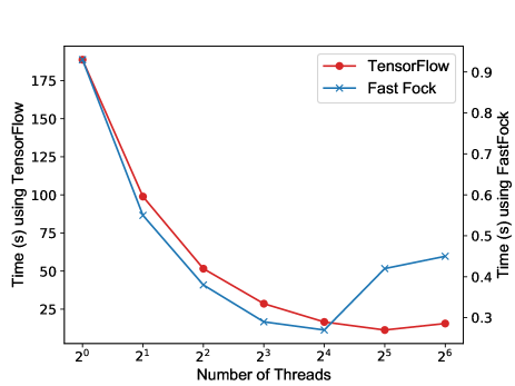
Figure 1: Time taken to evaluate the 24 Lagrangian gradients required for inverting the Hessian during the first finite-difference NR iteration of the Cl^--H₂O optimization.

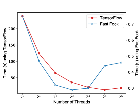
Figure 2: Time taken to evaluate the 22 Lagrangian gradients required for inverting the Hessian during the first finite-difference NR iteration of the NH₃-F₂ optimization.

III.2 Efficiency Gain and Cost Scaling

Here we compare the cost of two example ESMF optimizations when performed with our group’s previous AD-based implementation (denoted here as TensorFlow) with the new implementation based on analytic expressions and shell-pair screening (denoted here as FastFock). Working in the cc-pVDZ basis, Dunning (1988) we optimize the lowest singlet charged transfer excited states of the Cl^--H₂O dimer and the NH₃-F₂ dimer, both of which have been studied before. Zhao and Truhlar (2006); Zhao and Neuscamman (2020); Majumdar, Kim, and Kim (2000) The optimization uses the finite-difference NR approach, Shea, Gwin, and Neuscamman (2020) in which the NR linear equation is solved via the generalized minimal residual method (GMRES), with the Hessian-vector multiplication evaluated via a simple finite difference formula involving gradients of the objective function. In Figures 1 and 2, we compare the amount of time that the two implementations took to solve the linear equation for each optimization’s first NR step. Although we would clearly need to work with larger systems for our simple multi-threading approach to saturate the 32 cores on the processor, we see a roughly 100-fold increase in speed in both cases when running 16 threads (be careful to note the different left and right axes). When run in serial, the new implementation is 202 and 314 times faster than the TensorFlow implementation for the two different systems.

We now illustrate the origin of the efficiency of our new ESMF implementation by comparing the performance of the 5 different ESMF implementation options described in Table 2. These five implementations differ in programming language/framework, how they conduct differentiation, and whether shell-pair screening is performed. Option 1 is our old TensorFlow ESMF implementation and option 5 is our new FastFock implementation. Option 2-4 connect option 1 with option 5 by changing one variable at a time. We compare the amount of time each implementation took to evaluate the same 22 Lagrangian gradients in Figure 2.

Table 2: Comparison of how long five different ESMF implementations took to evaluate the Lagrangian gradients in Figure 2. The “Fock Build” column indicates which language the bottleneck Fock-build step is implemented in.

Option	Differentation	Fock Build	Shell-Pair Screening	Time (s)
1	Automatic	TensorFlow	No	35.64
2	Analytic	TensorFlow	No	3.41
3	Analytic	NumPy	No	3.69
4	Analytic	C	No	0.33
5	Analytic	C	Yes	0.35

As shown in the Table, by merely changing automatic differentiation to analytic differentiation but maintaining the TensorFlow framework, we already see a 10-fold speed-up in terms of the gradient evaluation. Such an acceleration shows the benefits of deriving analytic derivatives and collecting all the Fock-like matrices, since doing so allows us to drastically reduce the number of times we must access the memory-intensive two-electron integrals. Another 10-fold speed-up is achieved by moving the Fock build implementation from Python to C. In the final row, we see that this system is too small to benefit from shell-pair screening, and so we now turn our attention to larger cases in which this benefit can be realized.

In order to show the cost scaling of our method, in Figure 3 we plot the time taken to evaluate one Lagrangian gradient as a function of the number of orbitals in a NH₃-(H₂O)_n system. The structure is obtained by first putting water molecules around NH₃ randomly and then performing geometry optimizations in a 6-31G^∗ basis with MP2. As more water molecules are added, we find that the implementation’s cost scaling is roughly $O(N^{3})$. This is expected, as although the shell-pair screening can greatly reduce the cost of the Fock builds, the remaining matrix-matrix multiplications involved in forming our derivatives should give an $N^{3}$ scaling.

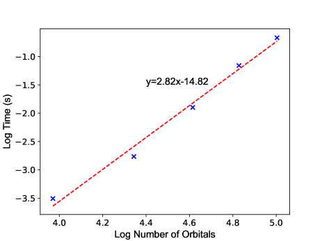
Figure 3: A log-log plot of the time taken to evaluate one Lagrangian gradient as a function of the number of atomic orbitals for the NH₃-(H₂O)_n system with varying numbers of water molecules. 8 OpenMP threads were used.

Table 3: Excitation energies (eV) for the TensorFlow and FastFock implementations, demonstrating that the shell-pair screening within the latter has not affected the energetics.

System	TensorFlow	Fast Fock
Cl--H2O	4.7195	4.7195
NH3-F2	4.5367	4.5367

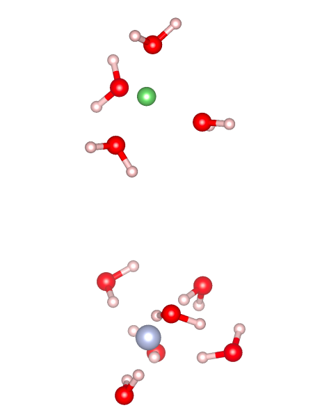
Figure 4: The geometry of the minimally-solvated charge transfer system, in which a Li atom surrounded by four water molecules can be seen above a F atom surrounded by six water molecules. The geometry was determined by two MP2 optimizations in the 6-31G^∗ basis, Petersson et al. (1988) one for the positively-charged Li cluster in isolation and one for the negatively-charged F cluster in isolation. The two clusters were then arranged one atop the other such that the Li and F atoms were 8.05$\mathring{A}$ apart. See Supplemental Materials for the atomic coordinates.

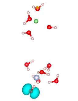
(a) CIS

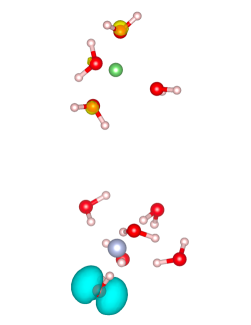
(b) TDDFT

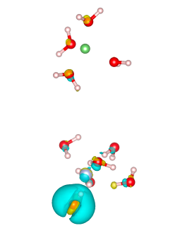
(c) ESMF

Figure 5: Isosurface plots for the charge density changes following the charge transfer excitation that moves an electron from the lower F cluster to the upper Li cluster, with blue surfaces showing charge depletion relative to the ground state and yellow surfaces showing charge accumulation. We compare the results using CIS, TDDFT, and ESMF in Figure 5(a), 5(b), and 5(c). TDDFT employed the $\omega$B97X functional. Note that the primary orbital on the Li cluster that accepts the transferred electron is very diffuse, and so at the isosurface value that makes charge-relaxation effects visible in the lower cluster the charge accumulation on the Li cluster is not visible. See the Supplemental Materials for a plot with an isosurface value that makes the Li cluster charge accumulation more clear.

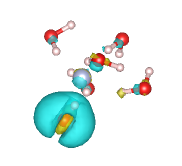
(a) ROHF

(b) UKS

(c) ESMF

Figure 6: As for Figure 5, but showing ROHF and UKS ground-state charge density differences between the neutral and negatively charged F cluster when modeled in isolation alongside ESMF’s charge density differences when it treats the charge transfer state in the full two-cluster system. We compare the results using ROHF, UKS, and ESMF in Figure 6(a), 6(b), and 6(c). UKS employed the $\omega$B97X functional.

Finally, in order to verify that the gain we obtained in efficiency does not come with a loss in accuracy from the shell-pair screening, we show the predicted excitation energies of Cl^--H₂O and NH₃-F₂ in Table 3. We found that the predictions match to better than 10^-4eV between the two implementations, indicating that there was no meaningful accuracy loss at the screening threshold we employed.

III.3 Minimally-solvated charge transfer

Table 4: Differences in atomic Mulliken charges for atoms in the lower cluster between the excited (lower cluster neutral) and ground (lower cluster negatively charged) states. For UKS, ROHF, and IP/EA-EOM-CCSD, we report the results for the corresponding charge states of the lower cluster in isolation (see text). DFT methods used the $\omega$B97X functional.

Method	F	O	H	H	O	H	H	O	H	H	O	H	H	O	H	H	O	H	H
CIS	0.01	0.01	0.00	0.00	0.00	0.00	0.00	0.00	0.00	0.00	0.96	0.01	0.01	0.00	0.00	0.00	0.00	0.00	0.00
TDDFT	0.01	0.00	0.00	0.00	0.00	0.00	0.00	0.00	0.00	0.00	0.96	0.01	0.01	0.00	0.00	0.00	0.00	0.00	0.00
UKS	0.06	0.04	0.00	0.02	0.11	0.01	0.03	0.10	0.03	-0.01	0.38	0.06	0.05	0.03	-0.01	0.01	0.08	0.01	0.03
ROKS	0.03	0.14	0.02	0.03	0.09	0.00	0.02	0.07	0.03	-0.01	0.32	0.06	0.05	0.04	-0.01	0.01	0.06	0.00	0.02
ROHF	0.01	0.02	-0.01	0.02	0.02	-0.02	0.01	0.02	0.03	-0.03	0.72	0.10	0.09	0.02	-0.01	0.01	0.02	-0.02	0.01
ESMF	0.01	0.03	-0.01	0.02	0.02	-0.02	0.01	0.01	0.03	-0.04	0.71	0.11	0.09	0.03	-0.01	0.00	0.02	-0.02	0.01
CCSD	0.02	0.01	-0.01	0.01	0.01	-0.01	0.00	0.01	0.01	-0.02	0.78	0.09	0.08	0.01	-0.01	0.00	0.01	-0.01	0.00

With these efficiency improvements in hand, we are able to make an initial investigation of ESMF’s predictions for how charge transfers in a minimally solvated environment. To this purpose, we study the system shown in Figure 4, in which a Li atom and a F atom are each surrounded by a small collection of water molecules. Although the geometry optimizations used a different basis (see figure), all subsequent calculations were performed in the cc-pVDZ orbital basis. When the two clusters are simulated as a single system with ground state methods, the F and Li clusters carry negative and positive net charges, respectively. Our purpose here is to investigate the predictions that various excited state methods make for how the charge density changes in the (lowest-energy singlet) charge transfer excitation that returns both clusters to charge neutrality.

As seen in Figure 5, the charge density changes predicted by ESMF differ noticeably from those of CIS and $\omega$B97X-based Chai and Head-Gordon (2008) TDDFT. Although all three methods (and all others tested, see below) agree that the transferred electron comes from a lone pair on the lower-left water molecule, ESMF also displays two types of significant orbital-relaxation effects that CIS and TDDFT fail to capture. First, electron density in the OH bonds on the affected water molecule is seen to shift towards the oxygen atom, showing a net charge depletion on the hydrogen atoms and some net charge accumulation close to the oxygen atom’s center. Second, the other water molecules show a polarization of their electron densities in response to the newly created hole on the lower-left water. As seen in Table 4, these relaxation effects create changes in the Mulliken populations for ESMF that differ significantly from those shown by CIS and TDDFT, both of which predict only significant changes to the lower-left oxygen atom.

Table 5: Comparison of excitation energies (eV) for the Li-F system’s charge transfer excitation. See text for details of the the CCSD approach.

Method	Excitation Energy
CIS	8.82
TDDFT/$\omega$B97X	6.12
ESMF	5.92
CCSD	6.64

At this point, we take advantage of the fact that the two clusters are well separated in order to perform IP/EA-EOM-CCSDSinha et al. (1988); Stanton and Gauss (1994); Nooijen and Barlett (1995) on the separate clusters in isolation in order to produce a high-level benchmark on what types of charge-relaxation effects other methods should display. As seen in Table 4, the coupled cluster predictions for the Mulliken population changes on both the lower-left water and the other water molecules agree reasonably well with the ESMF predictions while disagreeing with the CIS and TDDFT predictions. In particular, CIS and TDDFT fail to predict the significant relaxation near the lower-left water’s hydrogen atoms as well as the degree to which the charge densities on the other water molecules shift in response to the newly created hole. To verify that these errors are due to the additional approximations (namely a lack of secondary orbital relaxation) associated with CIS and TDDFT as excited state linear-response methods, we have also performed ground state restricted open-shell HF (ROHF) and $\omega$B97X-based unrestricted Kohn-Sham (UKS) calculations on the anionic and neutral lower cluster in isolation. As seen in Figure 6 and Table 4, these methods both display significant relaxation effects upon creation of the hole on the lower-left water, as should be expected of self-consistent field methods upon the removal of an electron. However, the ROHF and UKS predictions are quite different from each other, with the latter incorrectly delocalizing the hole across all of the water molecules in the lower cluster in a clear display of the difficulties posed by DFT’s self-interaction error, which is known to over-stabilize delocalized states. Lundberg and Siegbahn (2005); Cohen, Mori-Sánchez, and Yang (2008) ROHF, ESMF, and coupled cluster, in contrast, are by construction free of self-interaction errors and keep the hole localized on the lower-left water molecule, with the other water molecules showing much smaller net population changes while still correctly shifting their electron clouds to re-polarize after the creation of the hole. Note especially that the ROHF and ESMF results are in close agreement, which is not surprising given that the spin-purity offered by ESMF has only a very small energetic effect in this type of long-range charge transfer excitation. The same logic explains why the ROKS results are very similar to those of UKS, displaying the same clear signs of self-interaction-induced over-delocalization.

As a final note in this system, we remind the reader that ESMF, like HF, should not be expected to deliver highly accurate energetics as it neglects weak correlation effects. For the cluster under study, excitation energy estimates for different methods are shown in Table 5. Note that due to the large system size, we did not pursue a direct EOM-CCSD calculation in the full system. Instead, we created an estimate of the coupled cluster excitation energy via the expression

$$\Delta E=\mathrm{[EA]_{upper}}-\mathrm{[IP]_{lower}}+1/R$$ (21)

in which $\mathrm{[EA]_{upper}}$ is the electron affinity of the upper cluster in isolation and $\mathrm{[IP]_{lower}}$ is the ionization potential of the lower cluster in isolation, as predicted by IP/EA-EOM-CCSD. The $1/R$ term is used to estimate the Coulomb attraction of the two charged clusters in ground state, with $R$ computed as the distance between Li and F. As we have seen in many other systems, Shea, Gwin, and Neuscamman (2020) ESMF appears to underestimate the excitation energy. To reach quantitative energetics, a correlation correction such as the one provided by ESMP2 Shea, Gwin, and Neuscamman (2020) is clearly in order. While the current formulation and implementation of that theory is too expensive to use in a system of this size, work exploring more affordable formulations is ongoing.

III.4 More Charge Density Tests

Table 6: Differences in atomic Mulliken populations for atoms between the excited and ground states of NaCl. DFT methods used the $\omega$B97X functional.

Method	Na	Cl	total error
CIS	-0.93	0.93	0.41
TDDFT	-0.93	0.93	0.39
ROKS	-0.57	0.57	0.31
ESMF	-0.69	0.69	0.08
EOM-CCSD	-0.73	0.73	N/A

In light of ESMF’s success in predicting charge density changes in the previous section, we now turn our attention to how accurately the method predicts charge density changes in four additional charge transfer excitations. We examine charge transfer excitations in the NaCl molecule, the Cl^--(H₂O)₃ system, the C₂H₄-C₂F₄ dimer, and the aminophenol molecule. In these excitations, the charge flow is from Cl to Na, from Cl^- to H₂O, from C₂H₄ to C₂F₄, and from aminophenol’s OH and NH₂ groups to its benzene ring. Note that we provide the molecular structures and Cartesian coordinates of these test systems in the Supplemental Materials.

Tables 6, 7, 8, and 9 show how well ESMF, TDDFT, CIS, ROKS, and CIS do at predicting charge density differences in comparison to EOM-CCSD. Note that we use standard EOM-CCSD here on the full systems, as they are small enough for this to be practical, and that in some cases we use $\Delta$SCF instead of ROKS due to QChem’s current limitation of ROKS to HOMO/LUMO excitations. As their charge densities should be the same, we use the ROKS and $\Delta$SCF labels interchangeably in this section. We find that ESMF is consistently more accurate in these predictions than either CIS or TDDFT. When comparing ESMF and ROKS, we find that in three systems — Cl^--(H₂O)₃, C₂H₄-C₂F₄, and aminophenol — these methods’ accuracies are similar. However, for the charge density changes in NaCl and in the solvated charge transfer example of the previous section, ESMF is substantially more accurate than ROKS. The poorer performance of CIS and TDDFT can largely be explained by their inability to relax the orbitals not directly involved in the excitation. ROKS, on the other hand, does contain these types of relaxations through its $\Delta$SCF approach, but in some cases self-interaction error causes it to significantly overestimate the delocalization of the hole. We emphasize that we have employed a range-separated hybrid functional ($\omega$B97X) for TDDFT and ROKS in order to maximize their ability to deal successfully with charge transfer. Nonetheless, we find that ESMF is more reliable for predicting how the charge density changes in these charge transfer excitations.

IV Conclusion

We have presented explicit analytic expressions for the derivatives required for ESMF wave function optimization. Although these expressions are somewhat long winded, the upshot is that the necessary derivatives can be evaluated through nine Fock matrix builds and a collection of (much less expensive) single-particle matrix operations. This formulation allows ESMF to immediately benefit from methods that improve the efficiency of Fock builds, a situation we have exploited via the shell-pair screening strategy in order to construct a thread-parallel ESMF implementation that is multiple orders of magnitude faster than the previous implementation, which relied on automatic differentiation. We then applied our method to study a Li-F charge transfer system in which these atoms were surrounded by minimal water solvation shells. By comparing against IP/EA-EOM-CCSD, we found that ESMF’s predictions for how the charge transfer excitation changes the electron cloud were qualitatively more accurate than the predictions of CIS, TDDFT, UKS, or ROKS. In particular, ESMF correctly captured post-excitation orbital relaxation effects and, by virtue of being free of self-interaction errors, did not erroneously delocalize the hole.

Looking forward, these findings point to multiple priorities for further research. First, by giving ESMF access to larger systems, they make the development of an $N^{5}$-scaling post-ESMF perturbation theory (as opposed to the $N^{7}$-scaling of the existing Shea and Neuscamman (2018) version) even more pressing. Happily, a path forward in this direction has been found and will be published soon. Clune, Shea, and Neuscamman Second, we would expect the recently-introduced density functional extension to ESMF to show similar efficiency improvements upon development of Fock-build-based analytic gradients. Finally, in light of the efficiency offered by the successful generalization of the geometric direct minimization method to excited state orbital optimization, Hait and Head-Gordon (2019) it seems likely that employing our new analytic gradients in a custom-tailored quasi-Newton method would lead to further efficiency gains.

V Supplemental Material

See supplementary material for the molecular geometries, Cartesian coordinates, and overlap integrals between ground and excited states.

Table 7: Differences in atomic Mulliken populations for atoms between the excited and ground states of Cl^--(H₂O)₃. DFT methods used the $\omega$B97X functional.

Method	Cl	O	H	H	O	H	H	O	H	H	total error
CIS	0.86	0.04	-0.21	-0.09	0.07	-0.11	-0.24	0.04	-0.26	-0.09	0.32
TDDFT	0.88	0.01	-0.18	-0.13	0.04	-0.14	-0.19	0.02	-0.19	-0.13	0.25
ROKS	0.78	0.07	-0.21	-0.12	0.08	-0.12	-0.19	0.09	-0.24	-0.13	0.17
ESMF	0.85	0.06	-0.19	-0.14	0.07	-0.15	-0.21	0.08	-0.24	-0.15	0.16
EOM-CCSD	0.80	0.06	-0.18	-0.13	0.08	-0.14	-0.20	0.06	-0.21	-0.13	N/A

Table 8: Differences in atomic Mulliken populations for atoms between the excited and ground states of C₂H₄-C₂F₄. DFT methods used the $\omega$B97X functional.

Method	C	C	H	H	H	H	C	C	F	F	F	F	total error
CIS	0.49	0.49	0.00	0.00	0.00	0.00	-0.46	-0.46	-0.02	-0.02	-0.02	-0.02	1.30
TDDFT	0.49	0.49	0.00	0.00	0.00	0.00	-0.44	-0.44	-0.03	-0.03	-0.03	-0.03	1.19
ROKS	0.22	0.22	0.16	0.13	0.16	0.13	-0.28	-0.28	-0.10	-0.12	-0.10	-0.12	0.52
ESMF	0.24	0.24	0.15	0.12	0.15	0.12	-0.28	-0.28	-0.10	-0.12	-0.10	-0.12	0.45
EOM-CCSD	0.30	0.30	0.11	0.09	0.11	0.09	-0.33	-0.33	-0.08	-0.09	-0.08	-0.09	N/A

Table 9: Differences in atomic Mulliken populations for atoms between the excited and ground states of aminophenol. DFT methods used the $\omega$B97X functional.

Method	H	C	C	H	C	O	C	H	C	H	C	N	H	H	H	total error
CIS	-0.00	-0.10	-0.14	-0.00	0.10	0.05	-0.13	0.00	-0.07	0.00	0.12	0.12	0.00	0.00	0.00	0.57
TDDFT	-0.00	-0.11	-0.14	-0.00	0.11	0.09	-0.13	0.00	-0.09	0.00	0.07	0.19	0.00	0.00	0.00	0.60
ROKS	-0.02	-0.04	-0.06	-0.02	0.05	0.04	-0.06	-0.02	-0.03	-0.02	0.00	0.11	0.01	0.03	0.03	0.13
ESMF	-0.01	-0.04	-0.07	-0.02	0.07	0.03	-0.07	-0.02	-0.03	-0.01	0.00	0.11	0.01	0.03	0.03	0.18
EOM-CCSD	-0.01	-0.05	-0.06	-0.01	0.03	0.05	-0.05	-0.01	-0.04	-0.01	0.00	0.12	0.01	0.02	0.02	N/A

We provide the analytic expression of ESMF energy and target function derivatives in this section. Although the final results look tedious, the derivation is trivial as the ESMF energy and target function only involve matrix trace and products. Here we take the derivative of the first term in $E_{1}$ and $E_{2}$ with respect to $\Theta_{kp}$ for example,

$$\begin{split}&\frac{\partial}{\partial\Theta_{kp}}\left(2N_{2}\mathrm{Tr}[\bm{\Theta}\textbf{G}\bm{\Theta}^{T}]\right)\\ &=\frac{\partial}{\partial\Theta_{kp}}\left(2N_{2}\sum_{i}{[\bm{\Theta}\textbf{G}\bm{\Theta}]_{ii}}\right)\\ &=\frac{\partial}{\partial\Theta_{kp}}\left(2N_{2}\sum_{i}{\sum_{rs}{\Theta_{ir}G_{rs}\Theta_{is}}}\right)\\ &=2N_{2}\sum_{i}{\sum_{rs}{\Theta_{ir}G_{rs}\delta_{ki}\delta_{ps}}}+2N_{2}\sum_{i}{\sum_{rs}{\delta_{ki}\delta_{rp}G_{rs}\Theta_{is}}}\\ &=2N_{2}\sum_{r}{\Theta_{kr}G_{rp}}+2N_{2}\sum_{r}{G_{ps}\Theta_{ks}}\\ &=4N_{2}\left(\bm{\Theta}\textbf{G}\right)_{kp}\\ \end{split}$$ (22)

$$\begin{split}&\frac{\partial}{\partial\Theta_{kp}}\left(N_{2}\textbf{F}[\bm{\Theta}^{T}\bm{\Theta}]\cdot\left(\bm{\Theta}^{T}\bm{\Theta}\right)\right)\\ &=\frac{\partial}{\partial\Theta_{kp}}\left(N_{2}\sum_{rs}{\textbf{F}[\bm{\Theta}^{T}\bm{\Theta}]_{rs}\left(\bm{\Theta}^{T}\bm{\Theta}\right)_{rs}}\right)\\ &=N_{2}\sum_{rs}{\frac{\textbf{F}[\bm{\Theta}^{T}\bm{\Theta}]_{rs}}{\Theta_{kp}}\left(\bm{\Theta}^{T}\bm{\Theta}\right)_{rs}}+N_{2}\sum_{rs}{\textbf{F}[\bm{\Theta}^{T}\bm{\Theta}]_{rs}\frac{\left(\bm{\Theta}^{T}\bm{\Theta}\right)_{rs}}{\Theta_{kp}}}\end{split}$$ (23)

The derivative of the Fock matrix is

$$\begin{split}&\frac{\partial\textbf{F}[\bm{\Theta}^{T}\bm{\Theta}]_{rs}}{\partial\Theta_{kp}}\\ &=\frac{\partial}{\partial\Theta_{kp}}\left(2\textbf{J}[\bm{\Theta}^{T}\bm{\Theta}]_{rs}-\textbf{K}[\bm{\Theta}^{T}\bm{\Theta}]_{rs}\right)\\ &=2\sum_{v}{\Theta_{kv}(pv|rs)}+2\sum_{u}{\Theta_{ku}(pu|rs)}\\ &-\sum_{v}{\Theta_{kv}(rp|sv)}-\sum_{u}{\Theta_{ku}(ru|sp)}\\ \end{split}$$ (24)

Plugging this into the first term of Equation 22, we obtained

$$\begin{split}&N_{2}\sum_{rs}{\frac{\textbf{F}[\bm{\Theta}^{T}\bm{\Theta}]_{rs}}{\Theta_{kp}}\left(\bm{\Theta}^{T}\bm{\Theta}\right)_{rs}}\\ &=N_{2}\sum_{rs}{\left(\bm{\Theta}^{T}\bm{\Theta}\right)_{rs}[2\sum_{v}{\Theta_{kv}(pv|rs)}+2\sum_{u}{\Theta_{ku}(pu|rs)}]}\\ &-N_{2}\sum_{rs}{\left(\bm{\Theta}^{T}\bm{\Theta}\right)_{rs}[\sum_{v}{\Theta_{kv}(rp|sv)}+\sum_{u}{\Theta_{ku}(ru|sp)}]}\\ &=N_{2}\sum_{v}{\Theta_{kv}\textbf{F}[\bm{\Theta}^{T}\bm{\Theta}]_{pv}}+N_{2}\sum_{u}{\Theta_{ku}\textbf{F}[\bm{\Theta}^{T}\bm{\Theta}]_{pu}}\\ &=2N_{2}\left(\bm{\Theta}\textbf{F}[\bm{\Theta}^{T}\bm{\Theta}]\right)_{kp}\end{split}$$

The second term of Equation 22 is

$$\begin{split}&N_{2}\sum_{rs}{\textbf{F}[\bm{\Theta}^{T}\bm{\Theta}]_{rs}\frac{\left(\bm{\Theta}^{T}\bm{\Theta}\right)_{rs}}{\Theta_{kp}}}\\ &\sum_{rs}{\textbf{F}[\bm{\Theta}^{T}\bm{\Theta}]_{rs}\sum_{i}{\delta_{ki}\delta_{pr}\Theta_{is}}}+\sum_{rs}{\textbf{F}[\bm{\Theta}^{T}\bm{\Theta}]_{rs}\sum_{i}{\Theta_{ir}\delta_{ki}\delta_{ps}}}\\ &=2N_{2}\left(\bm{\Theta}\textbf{F}[\bm{\Theta}^{T}\bm{\Theta}]\right)_{kp}\\ \end{split}$$ (25)

Putting these together, we obtain

$$\frac{\partial}{\partial\Theta_{kp}}\left(N_{2}\textbf{F}[\bm{\Theta}^{T}\bm{\Theta}]\cdot\left(\bm{\Theta}^{T}\bm{\Theta}\right)\right)=4N_{2}\left(\bm{\Theta}\textbf{F}[\bm{\Theta}^{T}\bm{\Theta}]\right)_{kp}$$ (26)

The other terms of the energy and objective function derivatives could be computed in similar ways, and their expression are as follows.

The derivative with respect to $c_{0}$ is,

$$\begin{split}\frac{\partial E}{\partial c_{0}}&=\left(4c_{0}\mathrm{Tr}[\bm{\Theta}\textbf{ G}\bm{\Theta}^{T}]+4\mathrm{Tr}[\bm{\Theta}\textbf{G}\bm{\Gamma}^{T}\bm{\sigma}^{T}]\right.\\ &\left.+2c_{0}\textbf{F}[\bm{\Theta}^{T}\bm{\Theta}]\cdot\left(\bm{\Theta}^{T}\bm{\Theta}\right)+4\textbf{F}[\bm{\Theta}^{T}\bm{\Theta}]\cdot\left(\bm{\Theta}^{T}\bm{\sigma\Gamma}\right)\right)/N_{2}\\ &-2c_{0}E/N_{2}\\ \end{split}$$ (27)

The derivative with respect to $\sigma_{jb}$ is,

$$\begin{split}\frac{\partial E}{\partial\sigma_{jb}}&=\left(4c_{0}\left(\bm{\Theta}\textbf{G}\bm{\Gamma}^{T}\right)_{jb}+4\left(\bm{\sigma\Gamma}\textbf{G}\bm{\Gamma}^{T}\right)_{jb}\right.\\ &-4\left(\bm{\Theta}\textbf{G}\bm{\Theta}^{T}\bm{\sigma}\right)_{jb}+8\mathrm{Tr}[\bm{\Theta}\textbf{G}\bm{\Theta}^{T}]\sigma_{jb}\\ &+4c_{0}\left(\bm{\Theta}\textbf{F}[\bm{\Theta}^{T}\bm{\Theta}]\bm{\Gamma}^{T}\right)_{jb}+4\left(\bm{\sigma\Gamma}\textbf{F}[\bm{\Theta}^{T}\bm{\Theta}]\bm{\Gamma}^{T}\right)_{jb}\\ &-4\left(\bm{\Theta}\textbf{F}[\bm{\Theta}^{T}\bm{\Theta}]\bm{\Theta}^{T}\bm{\sigma}\right)_{jb}+4\left(\bm{\Theta}\textbf{F}[\bm{\Theta}^{T}\bm{\sigma\Gamma}]\bm{\Gamma}^{T}\right)_{jb}\\ &\left.+4\sum_{pq}{\left(\textbf{F}[\bm{\Theta}^{T}\bm{\Theta}]\bm{\Theta}^{T}\bm{\Theta}\right)_{pq}}\sigma_{jb}\right)/N_{2}\\ &-4E\sigma_{jb}/N_{2}\\ \end{split}$$ (28)

The derivative with respect to $\Theta_{kp}$ is,

$$\begin{split}\frac{\partial E}{\partial\Theta_{kp}}&=\left(4N_{2}\left(\bm{\Theta}\textbf{G}\right)_{kp}+4c_{0}\left(\bm{\sigma\Gamma}\textbf{G}\right)_{kp}\right.\\ &-4\left(\bm{\sigma\sigma}^{T}\bm{\Theta}\textbf{G}\right)_{kp}+4N_{2}\left(\bm{\Theta}\textbf{F}[\bm{\Theta}^{T}\bm{\Theta}]\right)_{kp}\\ &+4c_{0}\left(\bm{\sigma\Gamma}\textbf{F}[\bm{\Theta}^{T}\bm{\sigma\Gamma}]\right)_{kp}\\ &+4c_{0}\left(\bm{\Theta}\left(\textbf{F}[\bm{\Theta}^{T}\bm{\sigma\Gamma}]-F[\bm{\Theta}^{T}\bm{\sigma\Gamma}]^{T}\right)\right)_{kp}\\ &+2\left(\bm{\Theta}\left(\textbf{F}[\textbf{A}]-\textbf{F}[\textbf{A}]^{T}\right)\right)_{kp}-4\left(\bm{\sigma\sigma}^{T}\bm{\Theta}\textbf{F}[\bm{\Theta}^{T}\bm{\Theta}]\right)_{kp}\\ &\left.+4\left(\bm{\sigma\Gamma}\textbf{F}[\bm{\Theta}^{T}\bm{\sigma\Gamma}]\right)_{kp}/N_{2}\right)\\ \end{split}$$ (29)

The derivative with respect to $\Gamma_{cp}$ is,

$$\begin{split}\frac{\partial E}{\partial\Gamma_{cp}}&=\left(4c_{0}\left(\bm{\sigma}^{T}\bm{\Theta}\textbf{G}\right)_{cp}+4\left(\bm{\sigma}^{T}\bm{\sigma\Gamma}\textbf{G}\right)_{cp}\right.\\ &+4c_{0}\left(\bm{\sigma}^{T}\bm{\Theta}\textbf{F}[\bm{\Theta}^{T}\bm{\Theta}]\right)_{cp}+4\left(\bm{\sigma}^{T}\bm{\sigma\Gamma}\textbf{F}[\bm{\Theta}^{T}\bm{\Theta}]\right)_{cp}\\ &\left.+4\left(\bm{\sigma}^{T}\bm{\Theta}\textbf{F}[\bm{\Theta}^{T}\bm{\sigma\Gamma}]\right)_{cp}\right)\\ \end{split}$$ (30)

Let us now define different pieces of L,

$$\begin{split}L_{1}&=4c_{0}\mathrm{Tr}[\bm{\Theta}\textbf{G}\bm{\Theta}^{T}]+4\mathrm{Tr}[\bm{\Theta}\textbf{G}\bm{\Gamma}^{T}\bm{\sigma}^{T}]\\ &+2c_{0}F[\bm{\Theta}^{T}\bm{\Theta}]\cdot\left(\bm{\Theta}^{T}\bm{\Theta}\right)+4\textbf{F}[\bm{\Theta}^{T}\bm{\Theta}]\cdot\left(\bm{\Theta}^{T}\bm{\sigma\Gamma}\right)\\ L_{2}&=4c_{0}\mathrm{Tr}[\bm{\Theta}\textbf{G}\bm{\Gamma}^{T}\bm{\mu}^{T}]+4\mathrm{Tr}[\bm{\sigma\Gamma}\textbf{G}\bm{\Gamma}^{T}\bm{\mu}^{T}]\\ &-2\mathrm{Tr}[\bm{\Theta}\textbf{G}\bm{\Theta}^{T}\bm{\sigma\mu}^{T}+\bm{\Theta}\textbf{G}\bm{\Theta}^{T}\bm{\mu\sigma}^{T}]+8\bm{\sigma}\cdot\bm{\mu}\mathrm{Tr}[\bm{\Theta}\textbf{G}\bm{\Theta}^{T}]\\ &+4c_{0}\textbf{F}[\bm{\Theta}^{T}\bm{\Theta}]\cdot\left(\bm{\Theta}^{T}\bm{\mu\Gamma}\right)\\ &+2\textbf{F}[\bm{\Theta}^{T}\bm{\Theta}]\cdot\left(\bm{\Gamma}^{T}\bm{\sigma}^{T}\bm{\mu\Gamma}+\bm{\Gamma}^{T}\bm{\mu}^{T}\bm{\sigma\Gamma}-\bm{\Theta}^{T}\bm{\mu\sigma}^{T}\bm{\Theta}-\bm{\Theta}^{T}\bm{\sigma\mu}^{T}\bm{\Theta}\right)\\ &+4\left(\bm{\sigma}\cdot\bm{\mu}\right)\left(\textbf{F}[\bm{\Theta}^{T}\bm{\Theta}]\cdot\left(\bm{\Theta}^{T}\bm{\Theta}\right)\right)+4\textbf{F}[\bm{\Theta}^{T}\bm{\sigma\Gamma}]\cdot\left(\bm{\Theta}^{T}\bm{\sigma\Gamma}\right)\\ L_{3}&=4N_{2}\mathrm{Tr}[\textbf{RG}\bm{\Theta}^{T}]+4c_{0}\mathrm{Tr}[\textbf{RG}\bm{\Gamma}^{T}\bm{\sigma}^{T}]\\ &-2\mathrm{Tr}[\textbf{RG}\bm{\Theta}^{T}\bm{\sigma\sigma}^{T}+\bm{\Theta}\textbf{GR}^{T}\bm{\sigma\sigma}^{T}]\\ &+2N_{2}\left(\textbf{F}[\textbf{R}^{T}\bm{\Theta}]+\textbf{F}[\textbf{R}^{T}\bm{\Theta}]^{T}\right)\cdot\left(\bm{\Theta}^{T}\bm{\Theta}\right)\\ &+4c_{0}\left(\textbf{F}[\textbf{R}^{T}\bm{\Theta}]+\textbf{F}[\textbf{R}^{T}\bm{\Theta}]^{T}\right)\cdot\left(\bm{\Theta}^{T}\bm{\sigma\Gamma}\right)\\ &+4c_{0}\textbf{F}[\bm{\Theta}^{T}\bm{\Theta}]\cdot\left(\textbf{R}^{T}\bm{\sigma\Gamma}\right)\\ &+2\left(\textbf{F}[\textbf{R}^{T}\bm{\Theta}]+\textbf{F}[\textbf{R}^{T}\bm{\Theta}]^{T}\right)\cdot\textbf{A}\\ &-2\textbf{F}[\bm{\Theta}^{T}\bm{\Theta}]\cdot\left(\textbf{R}^{T}\bm{\sigma\sigma}^{T}\bm{\Theta}+\left(\textbf{R}^{T}\bm{\sigma\sigma}^{T}\bm{\Theta}\right)^{T}\right)\\ &+4\textbf{F}[\textbf{R}^{T}\bm{\sigma\Gamma}]\cdot\left(\bm{\Theta}^{T}\bm{\sigma\Gamma}\right)\\ &+4c_{0}\mathrm{Tr}[\bm{\Theta}\textbf{G}\bm{\Phi}^{T}\bm{\sigma}^{T}]+2\mathrm{Tr}[\bm{\sigma\Gamma}\textbf{G}\bm{\Phi}^{T}\bm{\sigma}^{T}+\left(\bm{\sigma\Gamma}\textbf{G}\bm{\Phi}^{T}\bm{\sigma}^{T}\right)^{T}]\\ &+4c_{0}\textbf{F}[\bm{\Theta}^{T}\bm{\Theta}]\cdot\left(\bm{\Theta}^{T}\bm{\sigma\Phi}\right)\\ &+2\textbf{F}[\bm{\Theta}^{T}\bm{\Theta}]\cdot\left(\bm{\Phi}^{T}\bm{\sigma}^{T}\bm{\sigma\Gamma}+\left(\bm{\Phi}^{T}\bm{\sigma}^{T}\bm{\sigma\Gamma}\right)^{T}\right)\\ &+4\textbf{F}[\bm{\Theta}^{T}\bm{\sigma\Gamma}]\cdot\left(\bm{\Theta}^{T}\bm{\sigma\Phi}\right)\end{split}$$ (31)

The derivatives of $L_{1}$, $L_{2}$, and $L_{3}$ with respect to $c_{0}$ are,

$$\begin{split}\frac{\partial L_{1}}{\partial c_{0}}&=4\mathrm{Tr}[\bm{\Theta}\textbf{G}\bm{\Theta}^{T}]+2\textbf{F}[\bm{\Theta}^{T}\bm{\Theta}]\cdot\left(\bm{\Theta}^{T}\bm{\Theta}\right)\\ \frac{\partial L_{2}}{\partial c_{0}}&=4\mathrm{Tr}[\bm{\Theta}\textbf{G}\bm{\Gamma}^{T}\bm{\mu}^{T}]+4F[\bm{\Theta}^{T}\bm{\Theta}]\cdot\left(\bm{\Theta}^{T}\bm{\mu\Gamma}\right)\\ \frac{\partial L_{3}}{\partial c_{0}}&=8c_{0}\mathrm{Tr}[\textbf{RG}\bm{\Theta}^{T}]+4\mathrm{Tr}[\textbf{RG}\bm{\Gamma}^{T}\bm{\sigma}^{T}]\\ &+4c_{0}\left(\textbf{F}[\textbf{R}^{T}\bm{\Theta}]+\textbf{F}[\textbf{R}^{T}\bm{\Theta}]^{T}\right)\cdot\left(\bm{\Theta}^{T}\bm{\sigma\Gamma}\right)\\ &+4\textbf{F}[\bm{\Theta}^{T}\bm{\Theta}]\cdot\left(\textbf{R}^{T}\bm{\sigma\Gamma}\right)\\ &+4\mathrm{Tr}[\bm{\Theta}\textbf{G}\bm{\Phi}^{T}\bm{\sigma}^{T}]+4\textbf{F}[\bm{\Theta}^{T}\bm{\Theta}]\cdot\left(\bm{\Theta}^{T}\bm{\sigma\Phi}\right)\end{split}$$ (32)

in which no new Fock build is needed.

The derivatives of $L_{1}$, $L_{2}$, and $L_{3}$ with respect to $\sigma_{jb}$ are,

$$\begin{split}\frac{\partial L_{1}}{\partial\sigma_{jb}}&=4\left(\bm{\Theta}\textbf{G}\bm{\Gamma}^{T}\right)_{jb}+4\left(\bm{\Theta}\textbf{F}[\bm{\Theta}^{T}\bm{\Theta}]\bm{\Gamma}^{T}\right)_{jb}\\ \frac{\partial L_{2}}{\partial\sigma_{jb}}&=4\left(\bm{\Gamma}\textbf{G}\bm{\Gamma}^{T}\bm{\mu}^{T}\right)^{T}_{jb}-4\left(\bm{\Theta}\textbf{G}\bm{\Theta}^{T}\bm{\mu}\right)_{jb}+8\mathrm{Tr}[\bm{\Theta}\textbf{G}\bm{\Theta}^{T}]\mu_{jb}\\ &+2\left(\bm{\mu\Gamma}\left(\textbf{F}[\bm{\Theta}^{T}\bm{\Theta}]+\textbf{F}[\bm{\Theta}^{T}\bm{\Theta}]^{T}\right)\bm{\Gamma}^{T}\right)_{jb}\\ &-2\left(\bm{\Theta}\left(\textbf{F}[\bm{\Theta}^{T}\bm{\Theta}]+\textbf{F}[\bm{\Theta}^{T}\bm{\Theta}]^{T}\right)\bm{\Theta}^{T}\bm{\mu}\right)_{jb}\\ &+4\textbf{F}[\bm{\Theta}^{T}\bm{\Theta}]\cdot\left(\bm{\Theta}^{T}\bm{\Theta}\right)\mu_{jb}+4\left(\bm{\Theta}\textbf{F}[\bm{\Theta}^{T}\bm{\mu\Gamma}]\bm{\Gamma}^{T}\right)_{jb}\\ \frac{\partial L_{3}}{\partial\sigma_{jb}}&=4c_{0}\left(\textbf{RG}\bm{\Gamma}^{T}\right)_{jb}-4\left(\textbf{RG}\bm{\Theta}^{T}\bm{\sigma}\right)_{jb}+16\mathrm{Tr}[\textbf{RG}\bm{\Theta}^{T}]\sigma_{jb}\\ &+4c_{0}\left(\bm{\Theta}\left(\textbf{F}[\textbf{R}^{T}\bm{\Theta}]+\textbf{F}[\textbf{R}^{T}\bm{\Theta}]^{T}\right)\bm{\Gamma}^{T}\right)_{jb}\\ &+4\left(\bm{\sigma\Gamma}\left(\textbf{F}[\textbf{R}^{T}\bm{\Theta}]+\textbf{F}[\textbf{R}^{T}\bm{\Theta}]^{T}\right)\bm{\Gamma}^{T}\right)_{jb}\\ &-4\left(\bm{\Theta}\left(\textbf{F}[\textbf{R}^{T}\bm{\Theta}]+\textbf{F}[\textbf{R}^{T}\bm{\Theta}]^{T}\right)\bm{\Theta}^{T}\bm{\sigma}\right)_{jb}\\ &+4c_{0}\left(\textbf{RF}[\bm{\Theta}^{T}\bm{\Theta}]\bm{\Gamma}^{T}\right)_{jb}\\ &-2\left(\textbf{R}\left(\textbf{F}[\bm{\Theta}^{T}\bm{\Theta}]+\textbf{F}[\bm{\Theta}^{T}\bm{\Theta}]^{T}\right)\bm{\Theta}^{T}\bm{\sigma}\right)_{jb}\\ &-2\left(\bm{\Theta}\left(\textbf{F}[\bm{\Theta}^{T}\bm{\Theta}]+\textbf{F}[\bm{\Theta}^{T}\bm{\Theta}]^{T}\right)\textbf{R}^{T}\bm{\sigma}\right)_{jb}\\ &+4\left(\textbf{RF}[\bm{\Theta}^{T}\bm{\sigma\Gamma}]\textbf{U}^{T}\right)_{jb}+4\left(\bm{\Theta}\textbf{F}[\textbf{R}^{T}\bm{\sigma\Gamma}]\bm{\Gamma}^{T}\right)_{jb}\\ &+8F[\Theta^{T}\Theta]\cdot\left(R^{T}\Theta+\theta R^{T}\right)\sigma_{jb}\\ &+4c_{0}\left(\Phi G\Theta^{T}\right)^{T}_{jb}+4\left(\Phi G\Gamma^{T}\sigma^{T}\right)^{T}_{jb}+4\left(\Gamma G\Phi^{T}\sigma^{T}\right)^{T}_{jb}\\ &+4c_{0}\left(\Theta F[\Theta^{T}\Theta]\Phi^{T}\right)_{jb}\\ &+2\left(\sigma\Phi\left(F[\Theta^{T}\Theta]+F[\Theta^{T}\Theta]^{T}\right)\Gamma^{T}\right)_{jb}\\ &+2\left(\sigma\Gamma\left(F[\Theta^{T}\Theta]+F[\Theta^{T}\Theta]^{T}\right)\Phi^{T}\right)_{jb}\\ &+4\left(\Theta\left(F[\Theta^{T}\sigma\Gamma]+F[\Theta^{T}\sigma\Gamma]^{T}\right)\Phi^{T}\right)_{jb}\\ &+4\left(\Theta\left(F[\Theta^{T}\sigma\Phi]+F[\Theta^{T}\sigma\Phi]^{T}\right)\Gamma^{T}\right)_{jb}\\ \end{split}$$ (33)

The derivatives of $L_{1}$, $L_{2}$, and $L_{3}$ with respect to $\Theta_{kp}$ are,

$$\begin{split}\frac{\partial L_{1}}{\partial\Theta_{kp}}&=8c_{0}\left(\Theta G\right)_{kp}+4\left(\sigma\Gamma G\right)_{kp}\\ &+8c_{0}\left(\Theta F[\Theta^{T}\Theta]\right)_{kp}+4\left(\sigma\Gamma F[\Theta^{T}\Theta]\right)_{kp}\\ &+4\left(\Theta\left(F[\Theta^{T}\sigma\Gamma]+F[\Theta^{T}\sigma\Gamma]^{T}\right)\right)_{kp}\\ \frac{\partial L_{2}}{\partial\Theta_{kp}}&=4c_{0}\left(\mu\Gamma G\right)_{kp}-4\left(\mu\sigma^{T}\Theta G\right)_{kp}+16\sigma\cdot\mu\left(\Theta G\right)_{kp}\\ &+4c_{0}\left(\mu\Gamma F[\Theta^{T}\Theta]^{T}\right)_{kp}\\ &+4c_{0}\left(\Theta\left(F[\Theta^{T}\mu\Gamma]+F[\Theta^{T}\mu\Gamma]^{T}\right)\right)_{kp}\\ &-4\left(\Theta\left(F[\Theta^{T}\mu\sigma^{T}\Theta]+F[\Theta^{T}\mu\sigma^{T}\Theta]^{T}\right)\right)_{kp}\\ &-2\left(\left(\mu\sigma^{T}\Theta+\sigma\mu^{T}\Theta\right)\left(F[\Theta^{T}\Theta]+F[\Theta^{T}\Theta]^{T}\right)\right)_{kp}\\ &+8\sigma\cdot\mu\left(\Theta\left(F[\Theta^{T}\Theta]+F[\Theta^{T}\Theta]^{T}\right)\right)_{kp}\\ &+4\left(\mu\Gamma F[\Theta^{T}\sigma\Gamma]^{T}\right)_{kp}+4\left(\sigma\Gamma F[\Theta^{T}\mu\Gamma]^{T}\right)_{kp}\\ \frac{\partial L_{3}}{\partial\Theta_{kp}}&=4N_{2}\left(RG\right)_{kp}-4\left(\sigma\sigma^{T}RG\right)_{kp}\\ &+2N_{2}\left(R\left(F[\Theta^{T}\Theta]+F[\Theta^{T}\Theta]^{T}\right)\right)_{kp}\\ &+4N_{2}\left(\Theta\left(F[R^{T}\Theta]+F[R^{T}\Theta]^{T}\right)\right)_{kp}\\ &+4c_{0}\left(R\left(F[\Theta^{T}\sigma\Gamma]+F[\Theta^{T}\sigma\Gamma]^{T}\right)\right)_{kp}\\ &+4c_{0}\left(\sigma\Gamma\left(F[R^{T}\Theta]+F[R^{T}\Theta]^{T}\right)\right)_{kp}\\ &+4c_{0}\left(\Theta\left(F[R^{T}\sigma\Gamma]+F[R^{T}\sigma\Gamma]^{T}\right)\right)_{kp}\\ &+4c_{0}\left(\Theta\left(F[\Theta^{T}\sigma\Phi]+F[\Theta^{T}\sigma\Phi]^{T}\right)\right)_{kp}\\ &+4c_{0}\left(\sigma\Phi F[\Theta^{T}\Theta]\right)_{kp}+2\left(R\left(F[A]+F[A]^{T}\right)\right)_{kp}\\ &-4\left(\sigma\sigma^{T}\Theta\left(F[R^{T}\Theta]+F[R^{T}\Theta]^{T}\right)\right)_{kp}\\ &+4\left(\Theta\left(F[B]+F[B]^{T}\right)\right)_{kp}\\ &-2\left(\sigma\sigma^{T}R\left(F[\Theta^{T}\Theta]+F[\Theta^{T}\Theta]^{T}\right)\right)_{kp}\\ &+4\left(\sigma\Gamma F[R^{T}\sigma\Gamma]^{T}\right)_{kp}\\ &+4\left(\sigma\Phi F[\Theta^{T}\sigma\Gamma]^{T}\right)_{kp}\\ &+4\left(\sigma\Gamma F[\Theta^{T}\sigma\Phi]^{T}\right)_{kp}\\ \end{split}$$ (34)

The derivatives of $L_{1}$, $L_{2}$, and $L_{3}$ with respect to $\Gamma_{cp}$ are,

$$\begin{split}\frac{\partial L_{1}}{\partial\Gamma_{cp}}&=4\left(\sigma^{T}\Theta G\right)_{cp}+4\left(\sigma^{T}\Theta F[\Theta^{T}\Theta]\right)_{cp}\\ \frac{\partial L_{2}}{\partial\Gamma_{cp}}&=4c_{0}\left(\mu\Gamma G\right)_{cp}-4\left(\mu\sigma^{T}\Theta G\right)_{cp}\\ &+4\left(\sigma^{T}\mu\Gamma G\right)_{cp}+4c_{0}\left(\mu^{T}\Theta F[\Theta^{T}\Theta]\right)_{cp}\\ &+2\left(\sigma^{T}\mu\Gamma\left(F[\Theta^{T}\Theta]+F[\Theta^{T}\Theta]^{T}\right)\right)_{cp}\\ &+2\left(\mu^{T}\sigma\Gamma\left(F[\Theta^{T}\Theta]+F[\Theta^{T}\Theta]^{T}\right)\right)_{cp}\\ &+4\left(\sigma^{T}\Theta F[\Theta^{T}\mu\Gamma]\right)_{cp}+4\left(\mu^{T}\Theta F[\Theta^{T}\sigma\Gamma]\right)_{cp}\\ \frac{\partial L_{3}}{\partial\Gamma_{cp}}&=4c_{0}\left(\sigma^{T}RG\right)_{cp}+4\left(\sigma^{T}\sigma\Phi G\right)_{cp}\\ &+4c_{0}\left(\sigma^{T}\Theta\left(F[R^{T}\Theta]+F[R^{T}\Theta]^{T}\right)\right)_{cp}\\ &+4\left(\sigma^{T}\sigma\Gamma\left(F[R^{T}\Theta]+F[R^{T}\Theta]^{T}\right)\right)_{cp}\\ &+4c_{0}\left(\sigma^{T}RF[\Theta^{T}\Theta]\right)_{cp}\\ &+4\left(\sigma^{T}RF[\Theta^{T}\sigma\Gamma]\right)_{cp}\\ &+4\left(\sigma^{T}\Theta F[R^{T}\sigma\Gamma]\right)_{cp}\\ &+2\left(\sigma^{T}\sigma\Phi\left(F[\Theta^{T}\Theta]+F[\Theta^{T}\Theta]^{T}\right)\right)_{cp}\\ &+4\left(\sigma^{T}\Theta F[\Theta^{T}\sigma\Phi]\right)_{cp}\\ \end{split}$$ (35)