All-order momentum correlations of three ultracold bosonic atoms confined in triple-well traps: Signatures of emergent many-body quantum phase transitions and analogies with three-photon quantum-optics interference

Abstract

All-order momentum correlation functions associated with the time-of-flight spectroscopy of three spinless ultracold bosonic interacting neutral atoms confined in a linear three-well optical trap are presented. The underlying Hamiltonian employed for the interacting atoms is an augmented three-site Hubbard model. Our investigations target matter-wave interference of massive particles, aiming at the establishment of experimental protocols for characterizing the quantum states of trapped attractively or repulsively interacting ultracold particles, with variable interaction strength. The manifested advantages and deep physical insights that can be gained through the employment of the results of our study for a comprehensive understanding of the nature of the quantum states of interacting many-particle systems, via analysis of the all-order (that is 1st, 2nd and 3rd) momentum correlation functions for three bosonic atoms in a three well confinement, are illustrated and discussed in the context of time-of-flight inteferometric interrogations of the interaction-strength-induced emergent quantum phase transition from the Mott insulating phase to the superfluid one. Furthermore, we discuss that our inteferometric interrogations establish strong analogies with the quantum-optics interference of three photons, including the aspects of genuine three-photon interference, which are focal to explorations targeting the development and implementation of quantum information applications and quantum computing.

I Introduction

Theoretical and experimental access to many-body correlations is essential in elucidating the properties and underlying physics of strongly interacting systems cira12 ; garc14 . In the framework of ultracold atoms, the quantum correlations in momentum space associated with bosonic or fermionic neutral atoms trapped in optical tweezers (with a finite number $N$ of particles prei19 ; berg19 ; bech20 ) or in extended optical lattices (with control of the 1D, 2D, or 3D dimensionality grei02 ; gerb05 ; gerb05.2 ; clem18 ; clem19 ) are currently attracting significant experimental attention, empowered bech20 ; prei19 ; berg19 ; clem18 ; clem19 ; hodg17 by advances in single-atom-resolved detection methods ott16 .

In this paper, we derive explicit analytic expressions for the 3rd-, 2nd-, and 1st-order momentum correlations of 3 ultracold bosonic atoms trapped in an optical trap of 3 wells in a linear arrangement (denoted as 3b-3w). Compared to the case of 2 particles in 2 wells (2p-2w) bran17 ; bran18 ; yann19.1 ; yann19.2 , a complete Hubbard-model treatment of momentum correlations (as a function of the interparticle interaction) for the 3b-3w case increases the complexity and effort involved, by an order of magnitude, because of the larger Hilbert space and the larger number of states, i.e., a total of 10 states instead of 4, including the excited states which are long-lived joch15 for trapped ultracold atoms. Therefore, demonstrating that this complexity of the theoretical treatment can be handled in an efficient manner through the use of algebraic computer languages constitutes an important step toward the implementation of the bottom-up approach for simulating many-body physics with ultracold atoms. In this respect, the statement above parallels earlier observations that three-particle entanglement extends two-particle entanglement in a nontrivial way zeil99 ; cira00 ; yann19.3 .

Compared to the standard numerical treatments galle15 ; rave17 ; shib72 ; call87 ; dago94 of the Hubbard model, the advantage of our algebraic treatment is the ability to produce in closed analytic form cosinusoidal/sinusoidal expressions of the many-body wave function and the associated momentum correlations of all orders; see for example Eqs. (44), (46), and (51), which codify the main results of our paper. Due to recent experimental advances in tunability and control of a system of a few ultracold atoms trapped in finite optical lattices (referred to also as optical tweezers), such momentum correlations can be measured directly in time-of-flight experiments berg19 ; prei19 ; bech20 and their experimental cosinusoidal diffraction patterns are revealing direct analogies with the quantum optics of massless photons bran18 ; yann19.1 ; prei19 .

In this context, this paper aims at researchers actively engaged in experimental and theoretical investigations of the properties of (finite) quantum few-body systems, as well as those aiming to understand many-body quantum systems through bottom-up hierarchical modeling of trapped finite ultracold-atom assemblies with deterministically controllable increased size and complexity; see, e.g., Refs. kauf14 ; kauf18 ; berg19 ; prei19 ; bech20 ; joch15 ; sowi16 ; zinn14 . Indeed, we target researchers in these fields by providing finger-print characteristics to aid the design, diagnostics, and interpretation of experiments, as well as by giving benchmark results note9 for comparisons with future theoretical treatments. We foresee these as important merits that will contribute to future impact of our work.

In addition, the availability of the complete analytic set of momentum correlations enabled us to reveal and explore two major physical aspects of the 3b-3w ultracold-atom system, namely: (i) Signatures of an emergent quantum phase transition note7 , from a Superfuid phase to a Mott-insulator phase – here the designation ’emergent’ is used to indicate the gradual emergence of a phase transition in a finite system as the system size is increased to infinity note7 , alternatively termed as ’inter-phase crossover’ – and (ii) Analogies between the interference properties of three trapped ultracold atom systems with quantum-optics three-photon interference. These aspects are elaborated in some detail immediately below.

(i) Signatures of emergent Superfluid to Mott transition: The sharp superfluid-to-Mott transition has been observed in extended optical lattices with trapped ultracold bosonic alkali atoms (⁸⁷Rb) grei02 , as well as with excited ⁴He^∗ bosonic atoms clem18 . In these experiments, after a time-of-flight (TOF) expansion, the single-particle momentum (spm) density (1st-order momentum correlation) was recorded. An oscillating spm-density provides a hallmark of a superfluid phase, associated with a maximum uncertainty regarding a particle’s site occupation; this happens for the non-interacting case when the particles are fully delocalized. On the other hand, a featureless spm-density is the hallmark of being deeply in the Mott-insulator phase when all particles are fully localized on the lattice sites exhibiting no fluctuations in the site occupancies.

Here, we show that the 1st-order momentum correlations for the 3b-3w system vary smoothly, alternating as a function of the Hubbard ${\cal U}$ between a featureless profile and that resulting from the sum of two cosine terms; such profile alternations may provide signatures of an emerging superfluid to Mott-insulator phase crossing. The periods of the cosine terms depend on the inverse of the lattice constant $d$ and its double $2d$ ($d$ being the nearest-neighbor interwell distance). We note that for extended lattices only the $\cos(dk)$ term has been theoretically specified gerb05.2 ; seng05 ; triv09 with perturbative $1/{\cal U}$ approaches, and that our non-perturbative results suggest that all cosine terms with all possible interwell distances in the argument should in general contribute.

Furthermore, we show that the correspondence between the featureless profiles and the interaction strength is not a one-to-one correspondence. Indeed, we show that a featureless spm-density can correspond to different strengths of the interaction, depending on the sign of the interaction (repulsive versus attractive) and the precise Hubbard state under consideration (ground state or one of the excited states). For a unique characterization of a phase regime, both the 2nd-order and the 3rd-order momentum correlations beyond the spm-density are required.

(ii) Analogies with quantum-optics three-photon interference: Recent experimental prei19 ; berg19 ; lege04 ; gerr15.1 ; gerr15.2 ; tamm18.1 ; tamm19 and theoretical bran17 ; bran18 ; bonn18 ; tamm18.2 ; yann19.1 ; yann19.2 ; yann19.3 advances have ushered a new research direction regarding investigations of higher-order quantum interference resolved at the level of the intrinsic microscopic variables that constitute the single-particle wave packet of the interfering particles. These intrinsic variables are pairwise conjugated; they are the single-particle momenta ($k$’s) and mutual distances ($d$’s) for massive localized particles prei19 ; berg19 ; bran17 ; bran18 ; bonn18 ; yann19.1 ; yann19.2 ; yann19.3 and the frequencies ($\omega$’s) and relative time delays ($\tau$’s) for massless photons lege04 ; gerr15.1 ; gerr15.2 ; tamm18.1 ; tamm18.2 ; tamm19 .

For the case of two fermionic or bosonic ultracold atoms, we investigated in Ref. yann19.1 this correspondence in detail and we proceeded to establish a complete analogy between the cosinusoidal patterns (with arguments $\propto kd$ or $\propto\omega\tau$) of the second-order $(k_{1},k_{2})$ correlation maps for the two trapped atoms (determined experimentally through TOF measurements prei19 ; berg19 ) with the landscapes of the two-photon ($\omega_{1},\omega_{2})$ interferograms gerr15.1 ; gerr15.2 ; tamm19 . In addition, we demonstrated that the Hong-Ou-Mandel (HOM) hom87 single-occupancy coincidence probability at the detectors, $P_{11}$ (which relates to the celebrated HOM dip for total destructive interference, i.e., when $P_{11}=0$), corresponds to a double integral over the momentum variables $(k_{1},k_{2})$ of a specific term contributing to the full correlation map, in full analogy with the treatment of the optical ($\omega_{1},\omega_{2})$ interferograms in Ref. gerr15.1 . Due to this summation over the intrinsic momentum (or frequency for photons) variables, the information contained in the HOM dip is limited compared to the full correlation map. Precise analogs of the original optical HOM dip (with $P_{11}$ varying as a function of relative time delay or separation between particles) have also been experimentally realized using the interference of massive particles, i.e., two colliding electrons taru98 ; jonc12 ; bocq13 or two colliding ⁴He atoms lope15 . For the case of two ultracold atoms trapped in two optical tweezers, analogs of the $P_{11}$ coincidence probability can be determined via in situ measurements, as a function of the time evolution of the system kauf14 ; yann19.1 or the interparticle interaction bran18 ; yann19.1 .

In this paper, we establish for the 3b-3w case the full range of analogies between the TOF spectroscopy note3 , as well as the in-situ measurements, of localized massive particles and the multi-photon interference in linear optical networks agar15 ; tamm18.1 ; tamm18.2 ; tamm19 , paying attention in particular to the mutual interparticle interactions which are absent for photons. These analogies encompass extensions of the 2p-2w analogies mentioned above, i.e., correlation maps dependent on three momentum variables $(k_{1},k_{2},k_{3})$ for massive particles versus interferograms with three frequency variables $(\omega_{1},\omega_{2},\omega_{3})$ for massless photons, and the HOM $P_{111}$ coincidence probability for three particles versus that for three photons. Most importantly, however, these analogies include highly nontrivial aspects beyond the reach of two-photon (or two-particle) and one-photon (or one-particle) interferences, such as genuine three-photon interference agne17 ; mens17 which cannot be determined from the knowledge solely of the lower two-photon and one-photon interferences.

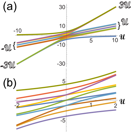
Figure 1: Spectrum of the ten bosonic eigenvalues in Eq. (9) as a function of ${\cal U}$ (horizontal axis). (a) This frame (with the extended $-10\leq{\cal U}\leq 10$ scale) illustrates the convergence to the three values of zero [ground state (${\cal U}>0$) or highest excited state (${\cal U}<0$)], $\pm|{\cal U}|$ (six excited states), and $\pm 3|{\cal U}|$ (ground state and two excited states for ${\cal U}<0$). (b) A more detailed view in the range $-2\leq{\cal U}\leq 2$. Taking into consideration the three energy crossings at ${\cal U}=0$, the corresponding eigenstates are labeled in ascending energy order as $i=1$, $2$, $3r(4l)$, $4r(3l)$, $5r(6l)$, $6r(5l)$, $7r(8l)$, $8r(7l)$, $9$, $10$, where “$r$” means “right” for the region of positive ${\cal U}$ and “$l$” means “left” for the region of negative ${\cal U}$.

I.1 Plan of paper

Following the introductory section where we defined the aims of this work, we introduce in Sec. II the linear three-site Hubbard model and its analytic solution for three spinless ultracold bosonic atoms. We display the spectrum of the ten bosonic eigenvalues of the Hubbard model for both attractive and repulsive interatomic interactions (Fig. 1), and discuss in detail: (1) the infinite repulsive or attractive interaction limit, and (2) the non-interacting limit. In Sec. III we outline the general definition and relations pertaining to higher-order correlations in momentum space.

In the following several sections we give explicit analytic results and graphical illustrations pertaining to momentum correlation functions of the various orders, starting from the third-order, since the lower-order are obtained from the third-order one by integration over the unresolved momentum variables [see, e.g., Eq. (45) for the second-order momentum correlation]. The third-order momentum correlations for 3 bosons in 3 wells, with explicit discussion of the infinite-interaction (repulsive or attractive) limit is given in Sec. IV (see Fig. 2), followed by explicit results for the non-interacting limit in Sec. V. Sec. VI is devoted to a presentation and discussion of results for the third-order momentum correlations for 3 bosons in 3 wells as a function of the strength of the inter-atom interaction over the whole range, from highly attractive to highly repulsive (see momentum correlation maps in Fig. 4). Next we discuss in Sec. VII the second-order momentum correlation as a function of the interparticle interaction; see momentum correlation maps for the whole interaction range in Fig. 6.

The first-order momentum correlation, obtained via integration of the second-order one over the momentum of one of the atoms, is discussed as a function of inter-atom interaction strength in Sec. VIII, with a graphic illustration in Fig. 8 for the first-excited state of 3 bosons in 3 wells, illustrating transition as a function of interaction strength from localized to superfluid behavior. Sec. IX is devoted to a detailed study of the quantum phase transition from localized to superfluid behavior, as deduced from inspection of the first-order correlation function for the ground state of 3 bosons in 3 wells (Fig. 9, top row), and further elucidated and elaborated with the use of second-order (Fig. 9, middle row), and third-order (Fig. 9, bottom row) momentum correlation maps. Further discussion of the quantum phase transition through analysis of site occupancies and their fluctuations for the ground and first-excited states as a function of the interparticle interactions, illuminating the connection between the quantum phase-transition from superfluid (phase coherent) to localized (incoherent) states, and the phase-number (site occupancy) uncertainty principle, is illustrated in Fig. 10.

Sec. X expounds on analogies with three-photon interference in quantum optics, including genuine three-photon interference. We summarize the contents of the paper in Sec. XI, closing with a comment concerning the expected relevance of the all-order momentum-space correlations for the 3 bosons in 3 wells as an alternative route to exploration with massive particles of aspects pertaining to the boson sampling problem aaar13 and its extensions, which are serving as a major topic (see, e.g., Refs. tamm15 ; tamm15.1 ; tich14 ; lain14 ; wals19 ) in quantum-optics investigations as an intermediate step towards the implementation of a quantum computer.

Appendix A and Appendix B complement Sec. II.1 and Sec. II.2, respectively, by listing the Hubbard eigenvectors of the remaining eight excited states not discussed in the main text (where, as above-mentioned, we focus on the ground and first-excited states). In addition, regarding again the remaining eight excited states not discussed in the main text, Appendix C and Appendix D complement Sec. IV and Sec. V, respectively, by listing the corresponding three-body wave functions. Specifically, Appendices A and C focus on the limit of infinite repulsive or attractive interaction, whereas Appendices B and D focus on the noninteracting case. The last three appendices give details of the all-order correlation functions as a function of the interaction strength for the remaining eight states not discussed in the main text.

II The linear three-site Hubbard model and its analytic solution for three spinless ultracold bosonic atoms

Numerical solutions for small Hubbard clusters are readily available in the literature. Here we present a compact analytic exposition for all the 10 eigenvalues and eigenstates of the linear three-bosons/three-site Hubbard Hamiltonian. Such analytic solutions, involving both the ground and excited states, are needed to further obtain the characteristic cosinusoidal or sinusoidal expressions for the associated third-, second-, and first-order momentum correlations.

The following ten primitive kets form a basis that spans the many-body Hilbert space of three spinless bosonic atoms distributed over three trapping wells:

$$\begin{split}&1\rightarrow\ket{111},\\ &2\rightarrow\ket{210},\;3\rightarrow\ket{201},\;4\rightarrow\ket{120},\\ &5\rightarrow\ket{021},\;6\rightarrow\ket{102},\;7\rightarrow\ket{012},\\ &8\rightarrow\ket{300},\;9\rightarrow\ket{030},\;10\rightarrow\ket{003}.\end{split}$$ (1)

The kets used above are of a general notation $|n_{1},n_{2},n_{3}\rangle$, where $n_{i}$ (with $i=1,2,3$) denotes the particle occupancy at the $i$th well. We note that there is only one primitive ket (No. 1) with all three wells being singly-occupied. The case of doubly-occupied wells is represented by 6 primitives kets (Nos. 2$-$7). Finally, there are 3 primitive kets (Nos. 8$-$10) that represent triply-occupied wells.

The Bose-Hubbard Hamiltonian for 3 spinless bosons trapped in 3 wells in a linear arrangement is given by

$$H_{B}=-J(\hat{b}^{\dagger}_{1}\hat{b}_{2}+\hat{b}^{\dagger}_{2}\hat{b}_{3}+h.c.)+\frac{U}{2}\sum_{i=1}^{3}n_{i}(n_{i}-1),$$ (2)

where $n_{i}=\hat{b}^{\dagger}_{i}\hat{b}_{i}$ is the occupation operator per site. $J$ is the hopping (tunneling) parameter and the Hubbard $U$ can be positive (repulsive interaction), vanishing (noninteracting), or negative (attractive interaction).

Using the capabilities of the SNEG sneg program in conjunction with the MATHEMATICA math18 algebraic language, one can write the following matrix Hamiltonian for the spinless three-boson Hubbard problem:

$$\begin{split}H_{b}=\left(\begin{array}[]{cccccccccc}0&0&-\sqrt{2}J&-\sqrt{2}J&-\sqrt{2}J&-\sqrt{2}J&0&0&0&0\\ 0&U&-J&-2J&0&0&0&-\sqrt{3}J&0&0\\ -\sqrt{2}J&-J&U&0&0&0&0&0&0&0\\ -\sqrt{2}J&-2J&0&U&0&0&0&0&-\sqrt{3}J&0\\ -\sqrt{2}J&0&0&0&U&0&-2J&0&-\sqrt{3}J&0\\ -\sqrt{2}J&0&0&0&0&U&-J&0&0&0\\ 0&0&0&0&-2J&-J&U&0&0&-\sqrt{3}J\\ 0&-\sqrt{3}J&0&0&0&0&0&3U&0&0\\ 0&0&0&-\sqrt{3}J&-\sqrt{3}J&0&0&0&3U&0\\ 0&0&0&0&0&0&-\sqrt{3}J&0&0&3U\\ \end{array}\right)\end{split}$$ (3)

The eigenvalues (in units of $J$) of the bosonic matrix Hamiltonian in Eq. (3) are:

$$\begin{array}[]{ll}E_{1}=\;{{}^{6}{\cal R}}^{b}_{1}&\;\;\;\;\;\;E_{6}=\;{{}^{3}{\cal R}}^{b}_{2}\;({\cal U})\\ E_{2}=\;{{}^{3}{\cal R}}^{b}_{1}&\;\;\;\;\;\;E_{7}=\;{{}^{6}{\cal R}}^{b}_{4}\\ E_{3}=\;{{}^{6}{\cal R}}^{b}_{2}&\;\;\;\;\;\;E_{8}=\;{{}^{6}{\cal R}}^{b}_{5}\\ E_{4}=\;{{}^{6}{\cal R}}^{b}_{3}&\;\;\;\;\;\;E_{9}=\;{{}^{3}{\cal R}}^{b}_{3}\\ E_{5}=\;{\cal U}\;({{}^{3}{\cal R}}^{b}_{2})&\;\;\;\;\;\;E_{10}=\;{{}^{6}{\cal R}}^{b}_{6},\end{array}$$ (9)

where ${\cal U}=U/J$. For $E_{5}$ and $E_{6}$, the quantities without parentheses apply for ${\cal U}>0$ and those within parentheses for ${\cal U}<0$. The expressions for the remaining eigenvalues apply for any ${\cal U}$, negative or positive. ${{}^{6}{\cal R}}^{b}_{i}$, $i=1,\ldots,6$ denote in ascending order (for any ${\cal U}$, negative or positive) the six real roots of the sixth-order polynomial

$$\begin{split}P^{b}_{6}(x)=&x^{6}-9{\cal U}x^{5}+(30{\cal U}^{2}-22)x^{4}\\ &+(144{\cal U}-46{\cal U}^{3})x^{3}+(76-314{\cal U}^{2}+33{\cal U}^{4})x^{2}-(252{\cal U}-264{\cal U}^{3}+9{\cal U}^{5})x-(72-180{\cal U}^{2}+72{\cal U}^{4}),\end{split}$$ (10)

and ${{}^{3}{\cal R}}^{b}_{i}$, $i=1,2,3$ denote in ascending order (for any ${\cal U}$, negative or positive) the three real roots of the third-order polynomial

$$P^{b}_{3}(x)=x^{3}-5{\cal U}x^{2}+(7{\cal U}^{2}-8)x+18{\cal U}-3{\cal U}^{3}.$$ (11)

Table 1:

Correspondence of the energy eigenvalues of the Hubbard matrix Hamiltonian [Eq. (3)] at the double degeneracies at ${\cal U}=0$; see Fig. 1. $E_{3}({\cal U}>0)$ $\Longleftrightarrow$ $E_{4}({\cal U}<0)$ $E_{4}({\cal U}>0)$ $\Longleftrightarrow$ $E_{3}({\cal U}<0)$ $E_{5}({\cal U}>0)$ $\Longleftrightarrow$ $E_{6}({\cal U}<0)$ $E_{6}({\cal U}>0)$ $\Longleftrightarrow$ $E_{5}({\cal U}<0)$ $E_{7}({\cal U}>0)$ $\Longleftrightarrow$ $E_{8}({\cal U}<0)$ $E_{8}({\cal U}>0)$ $\Longleftrightarrow$ $E_{7}({\cal U}<0)$

At ${\cal U}=0$, a smooth crossing of eigenvalues implies the correspondence displayed in TABLE 1, associated with the double degeneracies $E_{3}({\cal U}=0)=E_{4}({\cal U}=0)$, $E_{5}({\cal U}=0)=E_{6}({\cal U}=0)$, and $E_{7}({\cal U}=0)=E_{8}({\cal U}=0)$. These remarks are reflected in the choice of online colors (or shading in the print grayscale version) for the ${\cal U}>0$ and ${\cal U}<0$ segments of the curves in Fig. 1, where the bosonic eigenvalues listed in Eq. (9) are plotted as a function of ${\cal U}$. Note further that the ordering between $E_{4}$ and $E_{5}$ is interchanged for $|{\cal U}|\geq 3\sqrt{2}=4.24264$ [not visible in Fig. 1(a) due to the scale of the figure]. In the following, the corresponding Hubbard eigenstates are labeled in ascending energy order as $i=1$, $2$, $3r(4l)$, $4r(3l)$, $5r(6l)$, $6r(5l)$, $7r(8l)$, $8r(7l)$, $9$, $10$, where “$r$” means “right” for the region of positive ${\cal U}$ and “$l$” means “left” for the region of negative ${\cal U}$.

The 10 normalized eigenvectors $\phi^{b}_{i}({\cal U})$, with $i=1,\ldots,10$, of the bosonic matrix Hamiltonian in Eq. (3) have the general form

$$\begin{split}\phi&{}^{b}_{i}({\cal U})=\\ \{&{\bf c}_{111}({\cal U}),{\bf c}_{210}({\cal U}),{\bf c}_{201}({\cal U}),{\bf c}_{120}({\cal U}),{\bf c}_{021}({\cal U}),\\ &{\bf c}_{102}({\cal U}),{\bf c}_{012}({\cal U}),{\bf c}_{300}({\cal U}),{\bf c}_{030}({\cal U}),{\bf c}_{003}({\cal U})\}.\end{split}$$ (12)

Because the algebraic expressions for the ${\bf c}_{ijk}$’s for an arbitrary ${\cal U}$ are very long and complicated, we explicitly list in this paper the Hubbard eigenvectors only for the characteristic limits of infinite repulsive and attractive interaction (${\cal U}\rightarrow\pm\infty$) and for the non-interacting case (${\cal U}=0$). Specifically, for the reader’s convenience, we list in the main text only the Hubbard eigenvectors for the ground- and first-excited states; see Sec. II.1 and Sec. II.2. The eigenvectors for the remaining 8 excited states are given in Appendix A (for ${\cal U}\rightarrow\pm\infty$) and Appendix B (for ${\cal U}=0$).

II.1 The infinite repulsive or attractive interaction (${\cal U}\rightarrow\pm\infty$) limit

For large values of $|{\cal U}|$ (${\cal U}\rightarrow\pm\infty$), the ten bosonic eigenvalues in Eq. (9) (in units of $J$) are well approximated by the simpler expressions:

$$\begin{split}E_{1}^{+\infty}(E_{10}^{-\infty})=&\;-8/{\cal U}+20/{\cal U}^{3}\\ E_{2}^{+\infty}(E_{9}^{-\infty})=&\;{\cal U}\mp\sqrt{5}-3/(4{\cal U})\\ E_{3}^{+\infty}(E_{8}^{-\infty})=&\;{\cal U}\mp\sqrt{5}+33/(20{\cal U})\\ E_{4}^{+\infty}(E_{7}^{-\infty})=&\;{\cal U}+1/(5{\cal U})\\ E_{5}^{+\infty}(E_{6}^{-\infty})=&\;{\cal U}\\ E_{6}^{+\infty}(E_{5}^{-\infty})=&\;{\cal U}\pm\sqrt{5}-3/(4{\cal U})\\ E_{7}^{+\infty}(E_{4}^{-\infty})=&\;{\cal U}\pm\sqrt{5}+33/(20{\cal U})\\ E_{8}^{+\infty}(E_{3}^{-\infty})=&\;3{\cal U}+3/(2{\cal U})-9/(4{\cal U}^{3})\\ E_{9}^{+\infty}(E_{2}^{-\infty})=&\;3{\cal U}+3/(2{\cal U})+3/(4{\cal U}^{3})\\ E_{10}^{+\infty}(E_{1}^{-\infty})=&\;3{\cal U}+3/{\cal U}+7/(2{\cal U}^{3}),\end{split}$$ (13)

where symbols $E_{i}^{+\infty}$ without a parenthesis and the upper signs in $\mp$ and $\pm$ refer to the positive limit ${\cal U}\rightarrow+\infty$, and those ($E_{i}^{-\infty}$) within a parenthesis and the lower signs in $\mp$ and $\pm$ refer to the negative limit ${\cal U}\rightarrow-\infty$.

From the above, one sees that for large $\pm|{\cal U}|$ the bosonic eigenvalues are organized in three groups: a high-energy (low-energy) group of three eigenvalues around $\pm 3|{\cal U}|$ (triply occupied sites, see below), a middle-energy group of six eigenvalues around $\pm|{\cal U}|$ (doubly occupied sites, see below), and a single negative and lowest (positive and highest) eigenvalue approaching zero (singly occupied sites, see below). Fig. 1 illustrates this behavior.

The corresponding eigenvectors at ${\cal U}\rightarrow+\infty$ and ${\cal U}\rightarrow-\infty$ for the ground and first-excited states are given by

$$\begin{split}\phi^{b,+\infty}_{1}&=\{1,0,0,0,0,0,0,0,0,0\}\\ \phi^{b,-\infty}_{1}&=\{0,0,0,0,0,0,0,0,1,0\}\end{split}$$ (14)

$$\begin{split}\phi^{b,+\infty}_{2}&=\left\{0,-\frac{1}{2},-\frac{1}{2\sqrt{5}},-\frac{1}{\sqrt{5}},\frac{1}{\sqrt{5}},\frac{1}{2\sqrt{5}},\frac{1}{2},0,0,0\right\}\\ \phi^{b,-\infty}_{2}&=\{0,0,0,0,0,0,0,-\frac{1}{\sqrt{2}},0,\frac{1}{\sqrt{2}}\}\end{split}$$ (15)

The eigevectors for the remaining 8 excited states are listed in Appendix A. Note that the eigenvectors in Eqs. (14) and (15) and in Appendix A are grouped in pairs ($+\infty$, $-\infty$), which are displayed using a common equation number

The eigenvectors at ${\cal U}\rightarrow+\infty$ and ${\cal U}\rightarrow-\infty$ are pairwise related as follows:

$$\begin{array}[]{ll}\phi^{b,+\infty}_{1}=-\phi^{b,-\infty}_{10}&\;\;\;\;\;\;\phi^{b,+\infty}_{6}=-\phi^{b,-\infty}_{9}\\ \phi^{b,+\infty}_{2}=-\phi^{b,-\infty}_{5}&\;\;\;\;\;\;\phi^{b,+\infty}_{7}=-\phi^{b,-\infty}_{8}\\ \phi^{b,+\infty}_{3}=-\phi^{b,-\infty}_{4}&\;\;\;\;\;\;\phi^{b,+\infty}_{8}=\phi^{b,-\infty}_{3}\\ \phi^{b,+\infty}_{4}=\phi^{b,-\infty}_{7}&\;\;\;\;\;\;\phi^{b,+\infty}_{9}=\phi^{b,-\infty}_{2}\\ \phi^{b,+\infty}_{5}=\phi^{b,-\infty}_{6}&\;\;\;\;\;\;\phi^{b,+\infty}_{10}=\phi^{b,-\infty}_{1}\end{array}.$$ (21)

The pairs in Eq. (21) correspond to states with the same absolute eigenvalues $|E_{i}^{+\infty}|$ and $|E_{j}^{-\infty}|$ (with $i,j=1,\ldots,10$) given in Eq. (13).

II.2 The noninteracting (${\cal U}=0$) limit

When ${\cal U}=0$, the polynomial-root eigenvalues listed in Eq. (9) simplify to

$$\begin{array}[]{ll}E_{1}=\;-3\sqrt{2}&\;\;\;\;\;\;E_{6}=\;0\\ E_{2}=\;-2\sqrt{2}&\;\;\;\;\;\;E_{7}=\;\sqrt{2}\\ E_{3}=\;-\sqrt{2}&\;\;\;\;\;\;E_{8}=\;\sqrt{2}\\ E_{4}=\;-\sqrt{2}&\;\;\;\;\;\;E_{9}=\;2\sqrt{2}\\ E_{5}=\;0&\;\;\;\;\;\;E_{10}=\;3\sqrt{2}\end{array},$$ (27)

The ${\cal U}=0$ Hubbard ground-state eigenvector is given by

$$\begin{split}\phi_{1}^{b,{\cal U}=0}=\left\{\frac{\sqrt{3}}{4},\frac{\sqrt{\frac{3}{2}}}{4},\frac{\sqrt{3}}{8},\frac{\sqrt{3}}{4},\frac{\sqrt{3}}{4},\frac{\sqrt{3}}{8},\frac{\sqrt{\frac{3}{2}}}{4},\frac{1}{8},\frac{1}{2\sqrt{2}},\frac{1}{8}\right\}\end{split}$$ (28)

whereas the first-excited state is represented by the eigenvector

$$\begin{split}&\phi_{2}^{b,{\cal U}=0}=\\ &\left\{0,-\frac{1}{2},-\frac{1}{4\sqrt{2}},-\frac{1}{2\sqrt{2}},\frac{1}{2\sqrt{2}},\frac{1}{4\sqrt{2}},\frac{1}{2},-\frac{\sqrt{\frac{3}{2}}}{4},0,\frac{\sqrt{\frac{3}{2}}}{4}\right\}.\end{split}$$ (29)

The eigenvectors for the remaining 8 excited states are listed in Appendix B.

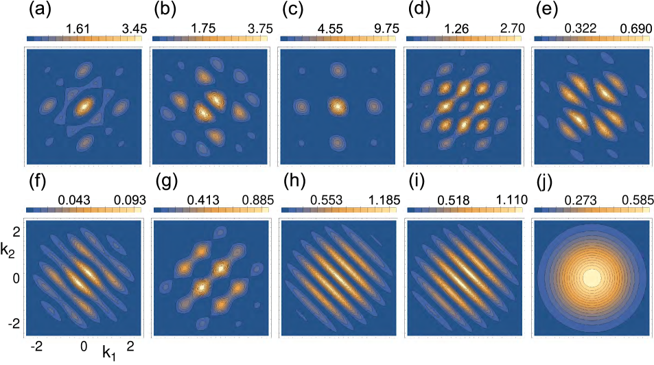
Figure 2: Cuts ($k_{3}=0$) of 3rd-order momentum correlation maps, ${}^{3}{\cal G}_{i}^{b,+\infty}=\Phi_{i}^{b,+\infty}\Phi_{i}^{b,+\infty,*}$, corresponding to the momentum-space wave functions for three bosons in three wells [see Eqs. (38)-(39) and Eqs. (83)-(90), top lines]. (a) Ground state ($i=1$). (b) First-excited sate ($i=2$). (c) Second-excited sate ($i=3$). (d) Third-excited sate ($i=4$). (e) Fourth-excited sate ($i=5$). (f) Fifth-excited sate ($i=6$). (g) Sixth-excited sate ($i=7$). (h) Seventh-excited sate ($i=8$). (i) Eighth-excited sate ($i=9$). (j) Ninth-excited sate ($i=10$). The choice of parameters is: interwell distance $d=3.8$ $\mu$m and spectral width of single-particle distribution in momentum space [see Eq. (35)] being the inverse of $s=0.5$ $\mu$m. The correlation functions ${}^{3}{\cal G}_{i}^{b,+\infty}(k_{1},k_{2},k_{3}=0)$ (map landscapes) are given in units of $\mu$m³ according to the color bars on top of each panel, and the momenta $k_{1}$ and $k_{2}$ are in units of 1/$\mu$m. The value of the plotted correlation functions was multiplied by a factor of 10 to achieve better contrast for the map features. 3rd-order momentum correlation maps for the infinite attractive limit are not explicitly plotted due to the equalities between pairs of the Hubbard eigenvectors at ${\cal U}\rightarrow-\infty$ and ${\cal U}\rightarrow+\infty$; see Eq. (21) for the detailed association of states.

III Higher-order correlations in momentum space: Outline of general definitions

To motivate our discussion about momentum-space correlation functions, it is convenient to recall that, usually, a configuration-interaction (CI) calculation (or other exact diagonalization schemes used for solution of the microscopic many-body Hamiltonian) yields a many-body wave function expressed in position coordinates. Then the $N$th-order real space density, $\rho(x_{1},x_{1}^{\prime},x_{2},x_{2}^{\prime},...,x_{N},x_{N}^{\prime})$, for an $N$-particle system is defined as the product of the many-body wave function $\Psi(x_{1},x_{2},\ldots,x_{N})$ and its complex conjugate $\Psi^{*}(x_{1}^{\prime},x_{2}^{\prime},\ldots,x_{N}^{\prime})$ lowd55 . The $i$th-order density function (with $i\leq N$) is defined as an integral over $\rho$ taken over the coordinates $x_{i+1},\ldots,x_{N}$ of $N-i$ particles, i.e.,

$$\begin{split}&\rho_{i}(x_{1},x_{1}^{\prime},x_{2},x_{2}^{\prime},\ldots,x_{i},x_{i}^{\prime})=\\ &\int dx_{i+1}\dots dx_{N}\rho(x_{1},x_{1}^{\prime},..,x_{i},x_{i}^{\prime},x_{i+1},x_{i+1},...x_{N},x_{N}).\end{split}$$ (30)

To obtain the $i$th-order real space correlation, one simply sets the prime coordinates in Eq. (30) to be equal to the corresponding unprimed ones,

$${}^{i}{\cal G}(x_{1},x_{2},...,x_{i})=\rho_{i}(x_{1},x_{1},x_{2},x_{2},...,x_{i},x_{i}).$$ (31)

Knowing the real-space density, one can obtain the corresponding higher-order momentum correlations through a Fourier transform bran17 ; bran18 ; yann19.1 ; alvi12

$$\begin{split}&{}^{i}{\cal G}(k_{1},k_{2},\ldots,k_{i})=\\ &\frac{1}{4\pi^{2}}\int e^{ik_{1}(x_{1}-x_{1}^{\prime})}e^{ik_{2}(x_{2}-x_{2}^{\prime})}\ldots e^{ik_{i}(x_{i}-x_{i}^{\prime})}\\ &\times\rho_{i}(x_{1},x_{1}^{\prime},x_{2},x_{2}^{\prime},\ldots,x_{i},x_{i}^{\prime})dx_{1}dx_{1}^{\prime}dx_{2}dx_{2}^{\prime}\ldots dx_{i}dx_{i}^{\prime},\end{split}$$ (32)

In this paper, we obtain directly an expression for the momentum-space $N$-body wave function corresponding to the Hubbard model Hamiltonian. This circumvents the need for the above Fourier-transform. Instead, consistent with the Fourier-transform relation [Eq. (32) above], the highest-order $N$th-order momentum correlation function is given by the modulus square

$${}^{N}{\cal G}(k_{1},k_{2},...,k_{N})=|\Phi(k_{1},k_{2},...,k_{N})|^{2},$$ (33)

and, successively, any lower $(N-i)$th-order (with $i=1,\ldots,N-1$) momentum correlation is obtained through an integration of the higher $(N-i+1)$th-order correlation over the $k_{N-i+1}$ momentum.

IV Third-order momentum correlations for 3 bosons in 3 wells: The infinite-interaction limit (${\cal U}\rightarrow\pm\infty$)

To derive the all-order momentum correlations, we augment the finite-site Hubbard model as follows: Each boson in any of the three wells is represented by a single-particle localized orbital having the form of a displaced Gaussian function bran17 ; bran18 ; yann19.1 ; yann19.3 , which in the real configuration space has the form

$$\psi_{j}(x)=\frac{1}{(2\pi)^{1/4}\sqrt{s}}\exp\left[-\frac{(x-d_{j})^{2}}{4s^{2}}\right].$$ (34)

In Eq. (34), $d_{j}$ ($j=1,2,3$) denotes the position of each of the three wells and $2s$ is the width of the Gaussian function in real configuration space. In this way, the structure (interwell distances) and the spatial profile of the orbitals of the trapped particles enter in the augmented Hubbard model. In momentum space, the corresponding orbital $\psi_{j}(k)$ is given by the Fourier transform of $\psi_{j}(x)$, namely, $\psi_{j}(k)=(1/\sqrt{2\pi})\int_{-\infty}^{\infty}\psi_{j}(x)\exp(ikx)dx$. Performing this Fourier transform, one finds

$$\psi_{j}(k)=\frac{2^{1/4}\sqrt{s}}{\pi^{1/4}}e^{-k^{2}s^{2}}e^{id_{j}k}.$$ (35)

Naturally the spectral witdth of the orbital’s profile in the momentum space is $1/s$.

In using orbitals localized on each well, our treatment of the augmented Hubbard trimer is similar to Coulson’s treatment of the Hydrogen molecule coul41 . In broader terms, our use of localized orbitals (atomic orbitals) belongs to the general methodology in chemistry known as LCAO-MO (linear combination of atomic orbitals $-$ molecular orbitals szabobook ; wiki2 ).

We stress that the cosinusoidal/sinusoidal dependencies of the momentum correlations derived here [and their coefficients ${\cal C}$’s, ${\cal B}$’s, and ${\cal A}$’s; see Eqs. (44), (46), and (51) below] do not depend on the precise profile of the atomic orbital, as noted already in Ref. coul41 , where the general symbol $\mathfrak{A}(k)$ was used for the Fourier transform of $\psi_{0}(x)$ at $d_{0}=0$. For the Hydrogen molecule an obvious choice is a Slater-type orbital (see Eqs. (35) and (36) in Ref. coul41 ). The reason behind this behavior is the so-called shift property shifttt of the Fourier transform, which applies to a displaced profile (centered at $d_{j}\neq 0$); it states that

$$\mathfrak{F}[\psi_{j}(x)]=\mathfrak{F}[\psi_{0}(x)]\exp(ikd_{j})=\mathfrak{A}(k)\exp(ikd_{j}),$$ (36)

where $\mathfrak{F}$ denotes the Fourier-transform operation shifttt . The Fourier-transformed profile $\mathfrak{A}(k)$ at the initial site factors out in all expressions of the momentum correlations. The Gaussian profile (also used in aforementioned experimental publications prei19 ; berg19 ; bech20 ; bonn18 ) in our paper was used for convenience; it is an obvious approximation for the lowest single-particle level in a deep potential note5 approaching a harmonic trap in the framework of experiments on neutral ultracold atoms note6 .

For a discussion of the comparison, for the entire range of interatomic interactions, ${\cal U}$, between exact microscopic diagonalization of the Hamiltonian (configuration interaction, CI) calculations, results of the augmented Hubbard-model, and measurements from trapped ultracold-atoms experiments, see Ref. note8 .

With the help of the single-boson orbitals in Eq. (35), each basis ket in Eq. (1) can be mapped onto a wave function of the three single-particle momenta $k_{1}$, $k_{2}$, and $k_{3}$. For each ket, this wave function naturally is a permanent built from the three bosonic orbitals. For a general eigenvector solution of the Hubbard Hamiltonian, the corresponding wave function $\Phi^{b}_{i}(k_{1},k_{2},k_{3})$ (with $i=1,\ldots,10$) in momentum space is a sum over such permanents, and the associated third-order correlation function is simply the modulus square, i.e.,

$${}^{3}{\cal G}^{b}_{i}(k_{1},k_{2},k_{3})=|\Phi^{b}_{i}(k_{1},k_{2},k_{3})|^{2}.$$ (37)

Because the expressions for the third-order correlations can become very long and cumbersome, for bookkeeping purposes, we found advantageous to display and characterize instead the three-body wave functions $\Phi^{b}_{i}(k_{1},k_{2},k_{3})$ themselves. Then the associated third-order correlations can be calculated using Eq. (37).

Below, in Eqs. (38)-(39), we list without commentary the momentum-space wave functions, $\Phi^{b,\pm\infty}_{1}(k_{1},k_{2},k_{3})$ and $\Phi^{b,\pm\infty}_{2}(k_{1},k_{2},k_{3})$, associated with the Hubbard eigenvectors, $\phi^{b,\pm\infty}_{1}$ and $\phi^{b,\pm\infty}_{2}$, respectively [see Eqs. (14)-(15)], at the limits of infinite repulsive or attractive strength (i.e., for ${\cal U}\rightarrow\pm\infty$). The commentary integrating these wave functions into the broader scheme of their evolution as a function of any interaction strength $-\infty<{\cal U}<+\infty$ is left for Sec. VI below. The three-body wave functions for the remaining 8 excited states are listed in Appendix C. Note that the wave functions in Eqs. (38) and (39) below and in Appendix C are grouped in pairs ($+\infty$, $-\infty$), which are displayed using a common equation number

Assuming that the wells are linearly placed at $d_{1}=-d$, $d_{2}=0$, and $d_{3}=d$, these momentum-space wave functions at ${\cal U}\rightarrow\pm\infty$ are as follows:

$$\begin{split}\Phi^{b,+\infty}_{1}(k_{1},k_{2},k_{3})&=\frac{2\times 2^{1/4}}{\sqrt{3}\pi^{3/4}}s^{3/2}e^{-(k_{1}^{2}+k_{2}^{2}+k_{3}^{2})s^{2}}[\cos(d(k_{1}-k_{2}))+\cos(d(k_{1}-k_{3}))+\cos(d(k_{2}-k_{3}))],\\ \Phi^{b,-\infty}_{1}(k_{1},k_{2},k_{3})&=\left(\frac{2}{\pi}\right)^{3/4}s^{3/2}e^{-(k_{1}^{2}+k_{2}^{2}+k_{3}^{2})s^{2}}.\end{split}$$ (38)

$$\begin{split}\Phi^{b,+\infty}_{2}(&k_{1},k_{2},k_{3})=\frac{i2^{3/4}}{5\sqrt{3}\pi^{3/4}}s^{3/2}e^{-(k_{1}^{2}+k_{2}^{2}+k_{3}^{2})s^{2}}\\ &\times\left[\sqrt{5}\sin(d(-k_{1}+k_{2}+k_{3}))+\sqrt{5}\sin(d(k_{1}+k_{2}-k_{3}))\right.+\sqrt{5}\sin(d(k_{1}-k_{2}+k_{3}))\\ &\;\;+5\sin(d(k_{1}+k_{2}))+5\sin(d(k_{1}+k_{3}))+5\sin(d(k_{2}+k_{3}))+2\sqrt{5}\sin(dk_{1})\left.+2\sqrt{5}\sin(dk_{2})+2\sqrt{5}\sin(dk_{3})\right],\\ \Phi^{b,-\infty}_{2}(&k_{1},k_{2},k_{3})=\frac{2i2^{1/4}}{\pi^{3/4}}s^{3/2}e^{-(k_{1}^{2}+k_{2}^{2}+k_{3}^{2})s^{2}}\sin(d(k_{1}+k_{2}+k_{3})).\end{split}$$ (39)

Plots for the corresponding 3rd-order momentum correlations ${}^{3}{\cal G}^{b,+\infty}_{i}(k_{1},k_{2},k_{3})$, with $i=1,\ldots,10$ [see Eq. (37)], are presented in Fig. 2. We note that we do not explicitly plot the 3rd-order momentum correlations for the limit of infinite attraction (${\cal U}\rightarrow-\infty$) because ${}^{3}{\cal G}^{b,-\infty}_{i}(k_{1},k_{2},k_{3})=^{3}{\cal G}^{b,+\infty}_{j}(k_{1},k_{2},k_{3})$ for the pairs $(i=1,j=10)$, $(i=2,j=9)$, $(i=3,j=8)$, $(i=4,j=3)$, $(i=5,j=2)$, $(i=6,j=5)$, $(i=7,j=4)$, $(i=8,j=7)$, $(i=9,j=6)$, and $(i=10,j=1)$ due to the equalities between eigenvectors listed in Eq. (21).

Explicit expression for the third-order correlation ${}^{3}{\cal G}^{b,+\infty}_{1}(k_{1},k_{2},k_{3})$. Because of the special role played by the ground state $\phi^{b,+\infty}_{1}=\ket{111}$ at infinite repulsion, we explicitly list below the corresponding third-order correlation function, i.e.,

$$\begin{split}&{}^{3}{\cal G}^{b,+\infty}_{1}(k_{1},k_{2},k_{3})=|\Phi^{b,+\infty}_{1}(k_{1},k_{2},k_{3})|^{2}=\\ &\frac{2\sqrt{2}}{3\pi^{3/2}}s^{3}e^{-2s^{2}(k_{1}^{2}+k_{2}^{2}+k_{3}^{2})}\big{\{}3+2\cos(d(k_{1}+k_{2}-2k_{3}))\\ &+2\cos(d(k_{2}+k_{3}-2k_{1}))+2\cos(d(k_{1}+k_{3}-2k_{2}))\\ &+\cos(2d(k_{1}-k_{2}))+2\cos(d(k_{1}-k_{2}))\\ &+\cos(2d(k_{1}-k_{3}))+2\cos(d(k_{1}-k_{3}))\\ &+\cos(2d(k_{2}-k_{3}))+2\cos(d(k_{2}-k_{3}))\big{\}}.\end{split}$$ (40)

It is worth noting that the expression (40) above for 3 bosons is similar to the third-order correlation for the triplet states (with total spin $S=3/2$ and spin projections $S_{z}=3/2$ or $S_{z}=1/2$) for 3-fermions trapped in 3 wells, except that in the fermionic case the sign in front of the cosine terms with only 2 momenta in the cosine argument is negative; see Refs. yann19.3 ; prei19

V Third-order momentum correlations for 3 bosons in 3 wells: The non-interacting limit ${\cal U}=0$

Assuming that the wells are linearly placed at $d_{1}=-d$, $d_{2}=0$, and $d_{3}=d$, the noninteracting ground-state three-boson wave function in momentum space is given by

$$\begin{split}&\frac{(2\pi)^{3/4}}{s^{3/2}}e^{(k_{1}^{2}+k_{2}^{2}+k_{3}^{2})s^{2}}\Phi_{1}^{b,{\cal U}=0}(k_{1},k_{2},k_{3})=1+2\sqrt{2}\cos(d{k_{1}})\cos(d{k_{2}})\cos(d{k_{3}})\\ &+2\cos(d{k_{1}})\cos(d{k_{2}})+2\cos(d{k_{1}})\cos(d{k_{3}})+\sqrt{2}\cos(d{k_{1}})+2\cos(d{k_{2}})\cos(d{k_{3}})+\sqrt{2}\cos(d{k_{2}})+\sqrt{2}\cos(d{k_{3}})\end{split}$$ (41)

The above takes also the form of the general expression (44) below, i.e.,

$$\begin{split}&\frac{(2\pi)^{3/4}}{s^{3/2}}e^{(k_{1}^{2}+k_{2}^{2}+k_{3}^{2})s^{2}}\Phi_{1}^{b,{\cal U}=0}(k_{1},k_{2},k_{3})=1+\sqrt{2}\big{(}\cos(dk_{1})+\cos(dk_{2})+\cos(dk_{3})\big{)}\\ &+\cos[d(k_{1}-k_{2})]+\cos[d(k_{1}-k_{3})]+\cos[d(k_{2}-k_{3})]+\cos[d(k_{1}+k_{2})]+\cos[d(k_{1}+k_{3})]+\cos[d(k_{2}+k_{3})]\\ &+\frac{1}{\sqrt{2}}\big{(}\cos[d(k_{1}+k_{2}-k_{3})]+\cos[d(k_{1}-k_{2}+k_{3})]+\cos[d(-k_{1}+k_{2}+k_{3})]+\cos[d(k_{1}+k_{2}+k_{3})]\big{)}\end{split}$$ (42)

For the first-excited state, the three-boson noninteracting wave function in momentum space at ${\cal U}=0$ was found to be

$$\begin{split}&\frac{-i(2\pi)^{3/4}\sqrt{3}}{s^{3/2}}e^{(k_{1}^{2}+k_{2}^{2}+k_{3}^{2})s^{2}}\Phi_{2}^{b,{\cal U}=0}(k_{1},k_{2},k_{3})=2\big{(}\sin(dk_{1})+\sin(dk_{2})+\sin(dk_{3})\big{)}\\ &+2\sqrt{2}\big{(}\sin[d(k_{1}+k_{2})]+\sin[d(k_{1}+k_{3})]+\sin[d(k_{2}+k_{3})]\big{)}\\ &+\sin[d(k_{1}-k_{2}+k_{3})]+\sin[d(-k_{1}+k_{2}+k_{3})]+\sin[d(k_{1}+k_{2}-k_{3})]+3\sin[d(k_{1}+k_{2}+k_{3})].\end{split}$$ (43)

The noninteracting three-body wave functions for the remaining 8 excited states are listed in Appendix D.

VI Third-order momentum correlations for 3 bosons in 3 wells as a function of the strength of the interaction ${\cal U}$

The general cosinusoidal (or sinusoidal) expression of third-order correlations is too cumbersome and lengthy to be displayed in print in a paper. Instead, as mentioned earlier, we give here the general expression for the three-boson wave function $\Phi_{i}^{b}(k_{1},k_{2},k_{3})$ (with $i=1,\ldots,10$) calculated in the momentum space. Then the third-order momentum correlations are obtained simply as the modulus square of this wave function [see Eq. (37)].

Using MATHEMATICA, we found that the general cosinusoidal (or sinusoidal) expression of the three-body wave function has the form:

$$\begin{split}&\Phi_{j}^{b}(k_{1},k_{2},k_{3})=p^{j}s^{3/2}e^{-(k_{1}^{2}+k_{2}^{2}+k_{3}^{2})s^{2}}\\ &\times\{{\cal C}_{0}^{j}+{\cal C}_{1}^{j}({\cal F}(dk_{1})+{\cal F}(dk_{2})+{\cal F}(dk_{3}))\\ &+{\cal C}_{1-1}^{j}({\cal F}[d(k_{1}-k_{2})]+{\cal F}[d(k_{1}-k_{3})]+{\cal F}[d(k_{2}-k_{3})])\\ &+{\cal C}_{1+1}^{j}({\cal F}[d(k_{1}+k_{2})]+{\cal F}[d(k_{1}+k_{3})]+{\cal F}[d(k_{2}+k_{3})])\\ &+{\cal C}_{1+1-1}^{j}({\cal F}[d(k_{1}+k_{2}-k_{3})]+{\cal F}[d(k_{1}-k_{2}+k_{3})]\\ &+{\cal F}[d(-k_{1}+k_{2}+k_{3})])+{\cal C}_{1+1+1}^{j}{\cal F}[d(k_{1}+k_{2}+k_{3})]\},\end{split}$$ (44)

where $p^{j}=1$ and ${\cal F}$ stands for “$\cos$” for the states $j=1,3r(4l),4r(3l),7r(8l),8r(7l),10$; $p^{j}=i$ (here $i^{2}=-1$; it is not an index) and ${\cal F}$ stands for “$\sin$” for the remaining states $j=2,5r(6l),6r(5l),9$. The ${\cal C}_{0}$ coefficient denotes an ${\cal F}$-independent term. The subscripts $1$, $1\pm 1$, and $1+1\pm 1$ in the other ${\cal C}$ coefficients reflect the number of terms in the argument of the ${\cal F}$ functions and the sign in front of each of them (without consideration of any ordering of the $k_{1}$, $k_{2}$, and $k_{3}$ momentum variables).

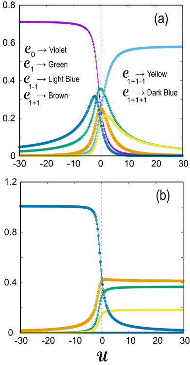
Figure 3: The six different ${\cal C}$-coefficients (dimensionless) [see Eq. (44)] for the 2 lowest-in-energy eigenstates of 3 bosons trapped in 3 linearly arranged wells as a function of ${\cal U}$ (dimensionless). (a) Ground state ($i=1$). (b) First-excited state ($i=2$). See text for a detailed description. For a description of the remaining eight excited states, see Appendix E. The choice of online colors is as follows: ${\cal C}_{0}\rightarrow$ Violet, ${\cal C}_{1}\rightarrow$ Green, ${\cal C}_{1-1}\rightarrow$ Light Blue, ${\cal C}_{1+1}\rightarrow$ Brown, ${\cal C}_{1+1-1}\rightarrow$ Yellow, ${\cal C}_{1+1+1}\rightarrow$ Dark Blue. For the print grayscale version, the positioning (referred to as #$n$, with $n=1,2,3,\dots$) of the curves from top to bottom at the point ${\cal U}=-6$ is as follows: (a) ${\cal C}_{0}\rightarrow$ #1, ${\cal C}_{1}\rightarrow$ #3, ${\cal C}_{1-1}\rightarrow$ #5, ${\cal C}_{1+1}\rightarrow$ #4, ${\cal C}_{1+1-1}\rightarrow$ #6, ${\cal C}_{1+1+1}\rightarrow$ #2 and (b) ${\cal C}_{0}=0$, ${\cal C}_{1}\rightarrow$ #3, ${\cal C}_{1-1}=0$, ${\cal C}_{1+1}\rightarrow$ #2, ${\cal C}_{1+1-1}\rightarrow$ #4, ${\cal C}_{1+1+1}\rightarrow$ #1.

In general, there are 14 cosinusoidal (or sinusoidal) terms and 6 distinct ${\cal U}$-dependent coefficients ${\cal C}$’s for a given state in expression (44). We note that ${\cal C}_{0}\equiv 0$ and ${\cal C}_{1-1}\equiv 0$ for any ${\cal U}$ for all the states of the second group above for which ${\cal F}\equiv\sin$. The ${\cal C}$-coefficients for the 2 lowest-in-energy eigenstates are plotted in Fig. 3 as a function of ${\cal U}$. The corresponding explicit numerical values can be found in a data file included in the supplemental material supp .

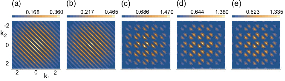
Figure 4: Cuts ($k_{3}=0$) of 3rd-order momentum correlation maps for the first-excited state of 3 bosons in 3 wells [see Eqs. (37) and (44) with $i=2$]. (a) ${\cal U}=-200$. (b) ${\cal U}=-10$. (c) ${\cal U}=0$. (d) ${\cal U}=10$. (e) ${\cal U}=200$. The choice of parameters is: interwell distance $d=7$ $\mu$m and spectral width of single-particle distribution in momentum space [see Eq. (35)] being the inverse of $s=0.35$ $\mu$m. The correlation functions ${}^{3}{\cal G}_{i}^{b}(k_{1},k_{2},k_{3}=0)$ (map landscapes) are given in units of $\mu$m³ according to the color bars on top of each panel, and the momenta $k_{1}$ and $k_{2}$ are in units of 1/$\mu$m. The value of the plotted correlation functions was multiplied by a factor of 10 to achieve better contrast for the map features.

Table 2: The 9 distinct coefficients at ${\cal U}=0$ present in Eq. (46) in the case of the ground state.

${\cal B}^{1,{\cal U}=0}_{0}$	${\cal B}^{1,{\cal U}=0}_{1}$	${\cal B}^{1,{\cal U}=0}_{2}$	${\cal B}^{1,{\cal U}=0}_{1-1}$	${\cal B}^{1,{\cal U}=0}_{2-2}$	${\cal B}^{1,{\cal U}=0}_{2-1}$	${\cal B}^{1,{\cal U}=0}_{1+1}$	${\cal B}^{1,{\cal U}=0}_{2+2}$	${\cal B}^{1,{\cal U}=0}_{2+1}$
$2/\pi=$	$2\sqrt{2}/\pi=$	$1/\pi=$	$2/\pi=$	$1/(4\pi)=$	$1/(\sqrt{2}\pi)=$	$2/\pi=$	$1/(4\pi)=$	$1/(\sqrt{2}\pi)=$
$0.63662$	$0.90032$	$0.31831$	$0.63662$	$0.07958$	$0.22508$	$0.63662$	$0.07958$	$0.22508$

The ground state (state denoted as $i=1$ for $-\infty<{\cal U}<+\infty$): For ${\cal U}\rightarrow-\infty$, it is seen from the panel (a) in Fig. 3 that only the constant coefficient ${\cal C}^{1,-\infty}_{0}=(2/\pi)^{3/4}=0.7127$ survives in expression (44); the ground-state in momentum space is given by the second expression in Eq. (38). It is a simple Gaussian distribution associated with a Bose-Einstein condensate, reflecting the fact that all three bosons are localized in the middle well and occupy the same orbital; the corresponding Hubbard eigenvector is given by $\phi^{b,-\infty}_{1}$ [second line in Eq. (14)] which contains only a single component from the primitive kets listed in Eq. (1), i.e., the basis ket No. 9 $\rightarrow|030\rangle$.

For ${\cal U}=0$, all 6 coefficients, ${\cal C}^{1,{\cal U}=0}$’s, are present, and their numerical values from the frame (a) in Fig. 3 agree with the corresponding algebraic expressions for $\Phi_{1}^{b,{\cal U}=0}(k_{1},k_{2},k_{3})$ in Eq. (42).

For ${\cal U}\rightarrow+\infty$, only the coefficient ${\cal C}^{1,+\infty}_{1-1}=2\times 2^{1/4}/(\sqrt{3}\pi^{3/4})=0.5819$ survives in expression (44); see again panel (a) in Fig. 3. The ground-state in momentum space comprises three cosinusoidal terms and is given by the first expression in Eq. (38). This form corresponds to the Hubbard eigenvector $\phi^{b,+\infty}_{1}$ [first line in Eq. (14)] which contains only a single component from the primitive kets listed in Eq. (1), i.e., the basis ket No. 1 $\rightarrow|111\rangle$.

As mentioned earlier, the primitive ket $|111\rangle$ represents a case where all three wells are singly occupied. Thus it enables a direct mapping to quantum-optics investigations of the frequency-resolved interference of three temporally distinguishable photons prepared in three separate fibers (tritter) tamm19 [recall the analogies yann19.1 : particle momentum ($k$) $\leftrightarrow$ photon frequency ($\omega/c$) and interwell distance ($d$) $\leftrightarrow$ time-delay between single photons ($\tau c$)].

The first excited state (state denoted as $i=2$ for $-\infty<{\cal U}<+\infty$): For ${\cal U}\rightarrow-\infty$ only the coefficient ${{\cal C}}^{2,-\infty}_{1+1+1}=2\times 2^{1/4}/\pi^{3/4}=1.0079$ survives in expression (44) [see frame (b) in Fig. 3]; the corresponding state, $\phi^{b,-\infty}_{2}$ [second line in Eq. (15)], is a NOON state of the form $(-|300\rangle+|003\rangle)/\sqrt{2}$, and the corresponding wave function in momentum space is given by the second expression in Eq. (39), which includes a single sin term only.

For ${\cal U}=0$, four coefficients are present, namely ${{\cal C}}^{2,{\cal U}=0}_{1}$, ${{\cal C}}^{2,{\cal U}=0}_{1+1}$, ${{\cal C}}^{2,{\cal U}=0}_{1+1-1}$, and ${{\cal C}}^{2,{\cal U}=0}_{1+1+1}$. Their numerical values from frame (b) in Fig. 3 agree with the corresponding algebraic expressions for $\Phi_{2}^{b,{\cal U}=0}(k_{1},k_{2},k_{3})$ in Eq. (43).

For ${\cal U}\rightarrow+\infty$ only three coefficients, ${{\cal C}}^{2,+\infty}_{1}=2\times 2^{3/4}/(\sqrt{15}\pi^{3/4})=0.3680$, ${{\cal C}}^{2,+\infty}_{1+1}=2^{3/4}/(\sqrt{3}\pi^{3/4})=0.4115$, and ${{\cal C}}^{2,+\infty}_{1+1-1}=2^{3/4}/(\sqrt{15}\pi^{3/4})=0.1840$, survive in expression (44) [see frame (b) in Fig. 3]; the corresponding state, $\phi^{b,+\infty}_{2}$ [first line in Eq. (15)] consists of all 6 primitive kets [see Eq. (1)] representing exclusively doubly-occupied wells, and the corresponding wave function in momentum space has 9 sinusoidal terms and is given by the first expression in Eq. (39).

In the main text of this paper, we restrict the ${\cal U}$-evolution of the ${\cal C}({\cal U})$’s coefficients in Eq. (44) to the two lowest-in-energy states. Indeed the ground state and the first excited state are the natural candidates for initial experiments. For example, for the case of two and three ultracold fermions (⁶Li atoms), see Ref. berg19 and Ref. prei19 , respectively; for recent experiments focused on the ground state of large bosonic Hubbard systems, see Refs. grei02 and gerb05.2 (⁸⁷Rb atoms) and Ref. clem18 ; clem19 (⁴He^∗ atoms). In the case of trapped ultracold atoms other excited states are in principle accessible. Thus in anticipation of future experimental activity, we complete in Appendix E the description of the details of the ${\cal U}$-evolution of the ${\cal C}({\cal U})$’s for the remaining eight excited states.

Fig. 4 illustrates visually for the first-excited state ($i=2$) the ${\cal U}$-evolution of the third-order correlation maps described by expressions (37) and (44) when $i=1$. The maps for 5 characteristic values of ${\cal U}$ are plotted, namely, ${\cal U}=-200$, $-10$, $0$, $10$, and $200$. Corresponding illustrations for the ground state are left for Sec. IX.

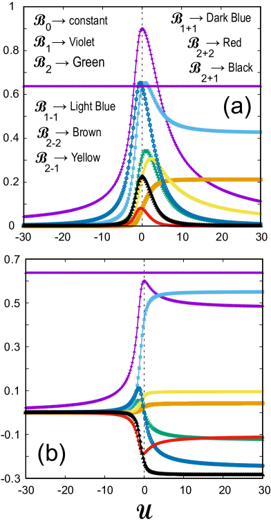
Figure 5: The ${\cal B}$-coefficients (dimensionless) [see Eq. (46)] for the 2 lowest-in-energy eigenstates of 3 bosons trapped in 3 linearly arranged wells as a function of the interaction strength ${\cal U}$ (dimensionless). (a) ground state ($i=1$). (b) First-excited state ($i=2$). See text for a detailed description. The choice of online colors is as follows: ${\cal B}_{0}\rightarrow$ Constant (Violet), ${\cal B}_{1}\rightarrow$ Second Violet, ${\cal B}_{2}\rightarrow$ Green, ${\cal B}_{1-1}\rightarrow$ Light Blue, ${\cal B}_{2-2}\rightarrow$ Brown, ${\cal B}_{2-1}\rightarrow$ Yellow, ${\cal B}_{1+1}\rightarrow$ Dark Blue, ${\cal B}_{2+2}\rightarrow$ Red, ${\cal B}_{2+1}\rightarrow$ Black. For the print grayscale version, the positioning (referred to as #$n$, with $n=1,2,3,\dots$) of the curves from top to bottom at the point ${\cal U}=+2$ is as follows: (a) ${\cal B}_{0}{\rm(constant)}\rightarrow$ #3, ${\cal B}_{1}\rightarrow$ #1, ${\cal B}_{2}\rightarrow$ #5, ${\cal B}_{1-1}\rightarrow$ #2, ${\cal B}_{2-2}\rightarrow$ #8, ${\cal B}_{2-1}\rightarrow$ #6, ${\cal B}_{1+1}\rightarrow$ #4, ${\cal B}_{2+2}\rightarrow$ #9, ${\cal B}_{2+1}\rightarrow$ #7 and (b) ${\cal B}_{0}{\rm(constant)}\rightarrow$ #1, ${\cal B}_{1}\rightarrow$ #2, ${\cal B}_{2}\rightarrow$ #6, ${\cal B}_{1-1}\rightarrow$ #3, ${\cal B}_{2-2}\rightarrow$ #5, ${\cal B}_{2-1}\rightarrow$ #4, ${\cal B}_{1+1}\rightarrow$ #7, ${\cal B}_{2+2}\rightarrow$ #8, ${\cal B}_{2+1}\rightarrow$ #9. For a description of the remaining eight excited states, see Appendix F.

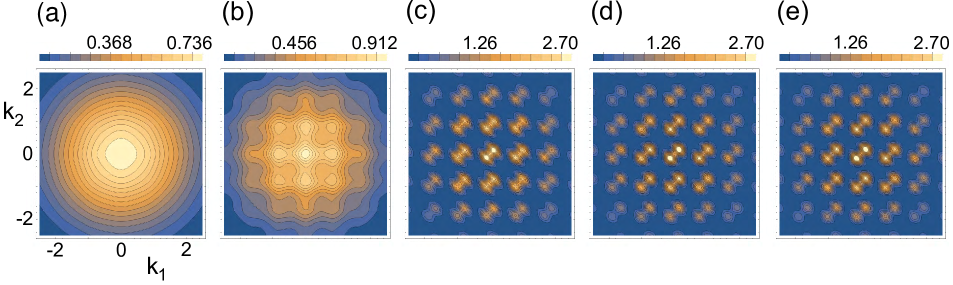
Figure 6: 2nd-order momentum correlation maps for the first-excited state of 3 bosons in 3 wells [see Eq. (46) with $i=2$]. (a) ${\cal U}=-200$. (b) ${\cal U}=-10$. (c) ${\cal U}=0$. (d) ${\cal U}=10$. (e) ${\cal U}=200$. The choice of parameters is: interwell distance $d=7$ $\mu$m and spectral width of single-particle distribution in momentum space [see Eq. (35)] being the inverse of $s=0.35$ $\mu$m. The correlation functions ${}^{2}{\cal G}_{i}^{b}(k_{1},k_{2})$ (map landscapes) are given in units of $\mu$m² according to the color bars on top of each panel, and the momenta $k_{1}$ and $k_{2}$ are in units of 1/$\mu$m. The value of the plotted correlation functions was multiplied by a factor of 10 to achieve better contrast for the map features.

Table 3: The 7 distinct coefficients at ${\cal U}=0$ present in Eq. (46) in the case of the 1st-excited state.

${\cal B}^{2,{\cal U}=0}_{0}$	${\cal B}^{2,{\cal U}=0}_{1}$	${\cal B}^{2,{\cal U}=0}_{2}$	${\cal B}^{2,{\cal U}=0}_{1-1}$	${\cal B}^{2,{\cal U}=0}_{2-2}$	${\cal B}^{2,{\cal U}=0}_{2-1}$	${\cal B}^{2,{\cal U}=0}_{1+1}$	${\cal B}^{2,{\cal U}=0}_{2+2}$	${\cal B}^{2,{\cal U}=0}_{2+1}$
$2/\pi=$	$4\sqrt{2}/\pi=$	0	$4/(3\pi)=$	$1/(12\pi)=$	$1/(3\sqrt{2}\pi)=$	0	$-7/(12\pi)=$	$-1/(\sqrt{2}\pi)=$
$0.63662$	$0.60021$		$0.42441$	$0.026526$	$0.075026$		$-0.185681$	$-0.22508$

Table 4: The 9 distinct coefficients at ${\cal U}\rightarrow+\infty$ present in Eq. (46) in the case of the 1st-excited state.

${\cal B}^{2,+\infty}_{0}$	${\cal B}^{2,+\infty}_{1}$	${\cal B}^{2,+\infty}_{2}$	${\cal B}^{2,+\infty}_{1-1}$	${\cal B}^{2,+\infty}_{2-2}$	${\cal B}^{2,+\infty}_{2-1}$	${\cal B}^{2,+\infty}_{1+1}$	${\cal B}^{2,+\infty}_{2+2}$	${\cal B}^{2,+\infty}_{2+1}$
$2/\pi$	$2\sqrt{5}/(3\pi)$	$-2/(5\pi)$	$26/(15\pi)$	$2/(15\pi)$	$2/(3\sqrt{5})$	$-4/(5\pi)$	$-1/(3\pi)$	$-2/(\sqrt{5}\pi)$

VII Second-order momentum correlations for 3 bosons in 3 wells as a function of the strength of the interaction ${\cal U}$

The second-order correlations are obtained through an integration of the third-order ones over the third momentum variable $k_{3}$, i.e.,

$${}^{2}{\cal G}_{i}^{b}(k_{1},k_{2})=\int^{\infty}_{-\infty}\;{}^{3}{\cal G}_{i}^{b}(k_{1},k_{2},k_{3})dk_{3},$$ (45)

with $i=1,\ldots,10$.

Using MATHEMATICA and neglecting the terms that vanish as $e^{-\gamma d^{2}/s^{2}}$ (for arbitrary $\gamma>0$ and $d^{2}/s^{2}>>1$), we found that the second-order correlations are given by the following general expression

$$\begin{split}&{}^{2}{\cal G}_{i}^{b}(k_{1},k_{2})=s^{2}e^{-2(k_{1}^{2}+k_{2}^{2})s^{2}}\\ &\times\{{\cal B}_{0}^{i}+{\cal B}_{1}^{i}(\cos(dk_{1})+\cos(dk_{2}))\\ &+{\cal B}_{2}^{i}(\cos(2dk_{1})+\cos(2dk_{2}))\\ &+{\cal B}_{1-1}^{i}\cos[d(k_{1}-k_{2})]+{\cal B}_{2-2}^{i}\cos[2d(k_{1}-k_{2})]\\ &+{\cal B}_{2-1}^{i}(\cos[d(k_{1}-2k_{2})]+\cos[d(2k_{1}-k_{2})])\\ &+{\cal B}_{1+1}^{i}\cos[d(k_{1}+k_{2})]+{\cal B}_{2+2}^{i}\cos[2d(k_{1}+k_{2})]\\ &+{\cal B}_{2+1}^{i}(\cos[d(k_{1}+2k_{2})]+\cos[d(2k_{1}+k_{2})])\}.\end{split}$$ (46)

The ${\cal B}_{0}$ coefficient denotes a $\cos$-independent term. The subscripts $1$, $2$, $1\pm 1$, $2\pm 1$, and $2\pm 2$ in the other ${\cal B}$ coefficients reflect the number of terms in the argument of the $\cos$ functions (one or two) and the factor of $\pm 1$ or $\pm 2$ in front of $k_{1}$ or $k_{2}$ (without consideration of any ordering of $k_{1}$ and $k_{2}$).

Including the constant term, there are 13 sinusoidal terms, but only 9 distinct coefficients in Eq. (46). The first coefficient above is a constant, i.e., ${\cal B}^{i}_{0}=2/\pi\approx 0.63662$ for all ten eigenstates. The remaining 8 ${\cal B}$-coefficients in Eq. (46) are ${\cal U}$-dependent. These ${\cal U}$-dependent ${\cal B}$-coefficients for the 2 lowest-in-energy eigenstates are plotted in Fig. 5 as a function of ${\cal U}$. The corresponding explicit numerical values can be found in a data file included in the supplemental material supp . Note that expression (46) has a total of 13 different cosine terms.

The ground state (state denoted as $i=1$ for $-\infty<{\cal U}<+\infty$): For ${\cal U}\rightarrow-\infty$ only the constant term, ${\cal B}^{1}_{0}$ survives; see the frame (a) in Fig. 5. The ground state is the triply occupied middle well [see the Hubbard eigenvector in the second line of Eq. (14)]. In this case, the second-order correlation function is

$${}^{2}{\cal G}_{1}^{b,-\infty}(k_{1},k_{2})=\frac{2}{\pi}s^{2}e^{-2(k_{1}^{2}+k_{2}^{2})s^{2}}.$$ (47)

In the noninteracting case (${\cal U}=0$), for which the Hubbard eigenvector is given by Eq. (28), all 13 cosinusoidal terms and 9 distinct coefficients (listed in TABLE 2) are present in Eq. (46), in agreement with frame (a) of Fig. 5.

For ${\cal U}\rightarrow+\infty$, three terms survive, including the constant one; see frame (a) in Fig. 5. In this case, the ground state is that of all three wells being singly occupied. In this case, the second-order correlation function acquires a simple expression

$$\begin{split}{}^{2}{\cal G}_{1}^{b,+\infty}&(k_{1},k_{2})=\frac{2}{3\pi}s^{2}e^{-2(k_{1}^{2}+k_{2}^{2})s^{2}}\{3\\ &+2\cos[d(k_{1}-k_{2})]+\cos[2d(k_{1}-k_{2})]\}.\end{split}$$ (48)

It is interesting to note that the second-order correlation function for three fermions with parallel spins trapped in three wells in the limit ${\cal U}\rightarrow+\infty$ is given by the same expression as that in Eq. (48), but with the 2 and 1 coefficients in front of the $\cos[d(k_{1}-k_{2})]$ and $\cos[2d(k_{1}-k_{2})]$ terms being replaced by their negatives, $-2$ and $-1$, respectively (see Eq. (9) and TABLE I (row for $i=3$) in Ref. yann19.3 ). This naturally is a reflection of the different quantum statistics between bosons and fermions.

Fig. 6 illustrates for the first-excited state the ${\cal U}$-evolution of the second-order correlation maps described by expression (46) when $i=2$. The maps for 5 specific values of ${\cal U}$ are plotted, namely, ${\cal U}=-200$, $-10$, $0$, $10$, and $200$.

The first excited state (state denoted as $i=2$ for $-\infty<{\cal U}<+\infty$): For ${\cal U}\rightarrow-\infty$ only the constant term, ${\cal B}^{2}_{0}=2/\pi$, survives; the corresponding state is a NOON state of the form $(-|300\rangle+|003\rangle)/\sqrt{2}$. In this case, the second-order correlation function is again

$${}^{2}{\cal G}_{2}^{b,-\infty}(k_{1},k_{2})=\frac{2}{\pi}s^{2}e^{-2(k_{1}^{2}+k_{2}^{2})s^{2}}.$$ (49)

In the noninteracting case (${\cal U}=0$), for which the Hubbard eigenvector is given by Eq. (29), 10 cosinusoidal terms and 7 distinct coefficients (listed in TABLE 3) are present in Eq. (46), in agreement with frame (b) of Fig. 5.

For ${\cal U}\rightarrow+\infty$, all 13 sinusoidal terms survive in expression (46); the corresponding state is given by the first expression in Eq. (15). For this case, we give the 9 distinct coefficients in TABLE 4.

These results are in agreement with the ${\cal U}$-dependence portrayed in frame (b) of Fig. 5.

For a description of the remaining eight excited states, see Appendix F.

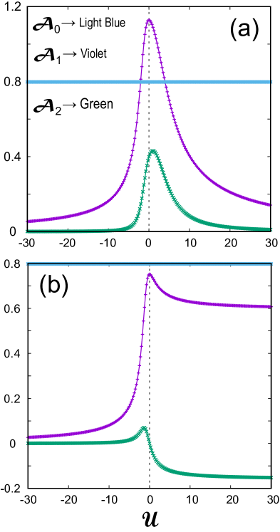
Figure 7: The ${\cal A}$-coefficients (dimensionless) [see Eq. (51)] for the 2 lowest-in-energy eigenstates of 3 bosons trapped in 3 linear wells as a function of the interaction strength ${\cal U}$ (dimensionless). (a) ground state ($i=1$). (b) First-excited state ($i=2$). See text for a detailed description. The choice of online colors is as follows: ${\cal A}_{0}\rightarrow$ Constant (Light Blue), ${\cal A}_{1}\rightarrow$ Violet, ${\cal A}_{2}\rightarrow$ Green. For the print grayscale version, excluding the top constant ${\cal A}_{0}$ horizontal line, the positioning of the two remaining curves in both frames is: ${\cal A}_{1}\rightarrow$ upper curve, ${\cal A}_{2}\rightarrow$ lower curve. For a description of the remaining eight excited states, see Appendix G.

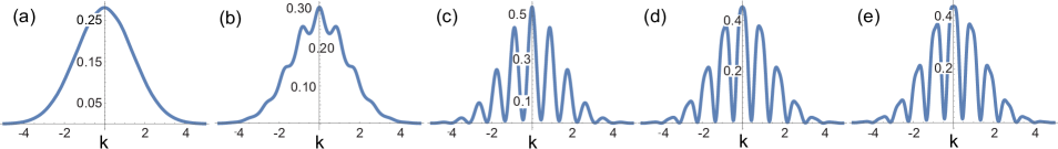
Figure 8: 1st-order momentum correlation plots for the first-excited state of 3 bosons in 3 wells. From left to right: (a) ${\cal U}=-200$, (b) ${\cal U}=-10$, (c) ${\cal U}=0$, (d) ${\cal U}=10$, and (e) ${\cal U}=200$ [see Eq. (51) with $i=2$]. The correlation functions ${}^{1}{\cal G}_{i}^{b}(k)$ (vertical axes) are given in units of $\mu$m, and the momenta $k$ are in units of 1/$\mu$m. The choice of parameters is: interwell distance $d=7$ $\mu$m and width of single-particle distribution in momentum space [see Eq. (35)] being the inverse of $s=0.35$ $\mu$m.

VIII First-order momentum correlations for 3 bosons in 3 wells as a function of the strength of the interaction ${\cal U}$

The first-order correlations are obtained through an integration of the second-order ones [see Eq. (46)] over the second momentum variable $k_{2}$, i.e.,

$${}^{1}{\cal G}_{i}^{b}(k)=\int^{\infty}_{-\infty}\;{}^{2}{\cal G}_{i}^{b}(k,k_{2})dk_{2},$$ (50)

with $i=1,\ldots,10$.

Exploiting the computational abilities of MATHEMATICA and neglecting terms that vanish as $e^{-\gamma d^{2}/s^{2}}$ (for arbitrary $\gamma>0$ and $d^{2}/s^{2}>>1$), one can find that the first-order correlations are given by the following general expression

$${}^{1}{\cal G}_{i}^{b}(k)=se^{-2k^{2}s^{2}}\{{\cal A}^{i}_{0}+{\cal A}^{i}_{1}\cos(dk)+{\cal A}^{i}_{2}\cos(2dk)\}.$$ (51)

${\cal A}^{i}_{0}=\sqrt{2/\pi}\approx 0.797885$ above is ${\cal U}$-independent for all ten eigenstates. The remaining two coefficients in Eq. (51), ${\cal A}^{i}_{1}$ and ${\cal A}^{i}_{2}$ are ${\cal U}$-dependent for 9 out of the ten eigenstates. These ${\cal U}$-dependent ${\cal A}$-coefficients for the 2 lowest-in-energy eigenstates are plotted as a function of ${\cal U}$ in Fig. 7. The corresponding explicit numerical values can be found in a data file included in the supplemental material supp .

The ground state (state denoted as $i=1$ for $-\infty<{\cal U}<+\infty$): For ${\cal U}\rightarrow-\infty$, it is seen from frame (a) in Fig. 7 that only the constant coefficient ${\cal A}^{1}_{0}$ survives in expression (51), i.e., the first-order correlation (single-particle density) in momentum space is devoid of any oscillatory structure, being given simply by a Gaussian distribution function,

$${}^{1}{\cal G}_{1}^{b,-\infty}(k)=\sqrt{\frac{2}{\pi}}se^{-2k^{2}s^{2}}.$$ (52)

This structureless distribution corresponds to a photonic triple-slit experiment where Young’s youn04 “which way” question, related to the source of the particle detected with a time-of-flight measurement, can be answered with a 100% certainty as being one single well (zero quantum fluctuations in the single-particle occupation number per site). Indeed, the corresponding ground-state Hubbard eigenvector is given by $\phi^{b,-\infty}_{1}$ [second line in Eq. (14)] which contains only one triply-occupied component from the primitive kets listed in Eq. (1), i.e., the basis ket No. 9 $\rightarrow|030\rangle$.

For the non-interacting case (${\cal U}=0$), all 3 coefficients survive [see frame (a) in Fig. 7]; specifically one has:

$${}^{1}{\cal G}_{1}^{b,{\cal U}=0}(k)=\sqrt{\frac{2}{\pi}}se^{-2k^{2}s^{2}}\{1+\sqrt{2}\cos(dk)+\frac{1}{2}\cos(2dk)\}.$$ (53)

Expression (53) exhibits a highly oscillatory interference pattern. It corresponds to the ground state given by the Hubbard eigenvector in Eq. (28), which is often described as a bosonic superfluid. Indeed the quantum fluctuations in the single-particle occupation number per site are strongest and the single-particle bosonic orbitals are maximally delocalized over all three sites.

For ${\cal U}\rightarrow+\infty$, it is seen from frame (a) in Fig. 7 that again only the ${\cal U}$-independent coefficient ${\cal A}^{1}_{0}$ survives in expression (51), i.e., the first-order correlation (single-particle density) in momentum space is devoid of any oscillatory structure, being given simply by a Gaussian distribution function like in Eq. (52), i.e.,

$${}^{1}{\cal G}_{1}^{b,+\infty}(k)={{}^{1}{\cal G}}_{1}^{b,-\infty}(k).$$ (54)

Again, this structureless distribution corresponds to a photonic triple-slit experiment where Young’s youn04 “which way” question, related to the source of the particle detected with a time-of-flight measurement, can be answered with a 100% certainty as being one single well (zero quantum fluctuations in the single-particle occupation number per site). Indeed, the corresponding ground-state Hubbard eigenvector is given by $\phi^{b,+\infty}_{1}$ [first line in Eq. (14)] which contains only the singly-occupied component from the primitive kets listed in Eq. (1), i.e., the basis ket No. 1 $\rightarrow|111\rangle$. The implications of the above results encoded in Eqs. (52), (53), and (54) regarding phase transitions will be discussed below in Sec. IX.

The first excited state (state denoted as $i=2$ for $-\infty<{\cal U}<+\infty$): For ${\cal U}\rightarrow-\infty$, it is seen from frame (b) in Fig. 7 that only the constant coefficient ${\cal A}^{1}_{0}$ survives in expression (51), i.e., the first-order correlation (single-particle density) in momentum space is devoid of any oscillatory structure, being given simply by a Gaussian distribution function,

$${}^{1}{\cal G}_{2}^{b,-\infty}(k)=\sqrt{\frac{2}{\pi}}se^{-2k^{2}s^{2}}.$$ (55)

In this case, this structureless distribution does not correspond to zero quantum fluctuations in the single-particle occupation number per site (see detailed discussion in Sec. IX below). Indeed, the corresponding Hubbard eigenvector is given by $\phi^{b,-\infty}_{2}$ [second line in Eq. (15)] which is a NOON state spread over two sites. i.e., it is a superposition of the two basis kets No. 8 $\rightarrow|300\rangle$ and No. 10 $\rightarrow|003\rangle$.

For the non-interacting case (${\cal U}=0$), 2 coefficients survive [see frame (b) in Fig. 7]; specifically one has:

$${}^{1}{\cal G}_{2}^{b,{\cal U}=0}(k)=\sqrt{\frac{2}{\pi}}se^{-2k^{2}s^{2}}\{1+\frac{2\sqrt{2}}{3}\cos(dk)\}.$$ (56)

Expression (56) exhibits a highly oscillatory interference pattern. It corresponds to the state given by the Hubbard eigenvector in Eq. (29).

For ${\cal U}\rightarrow+\infty$, all 3 coefficients survive [see frame (b) in Fig. 7], one of them being negative; specifically one has:

$${}^{1}{\cal G}_{2}^{b,+\infty}(k)=\sqrt{\frac{2}{\pi}}se^{-2k^{2}s^{2}}\{1+\frac{\sqrt{5}}{3}\cos(dk)-\frac{1}{5}\cos(2dk)\}.$$ (57)

Expression (57) exhibits a highly oscillatory interference pattern. It corresponds to the state given by the Hubbard eigenvector in the first line of Eq. (15), which consists exclusively of double-single occupancy components [basis kets No. 2 to No. 7; see Eq. (1)]

Fig. 8 illustrates for the first-excited state the ${\cal U}$-evolution of the first-order correlations described by expression (51) when $i=2$. The cases for 5 characteristic values of ${\cal U}$ are plotted, namely, ${\cal U}=-200$, $-10$, $0$, $10$, and $200$.

For a description of the remaining eight excited states, see Appendix G.

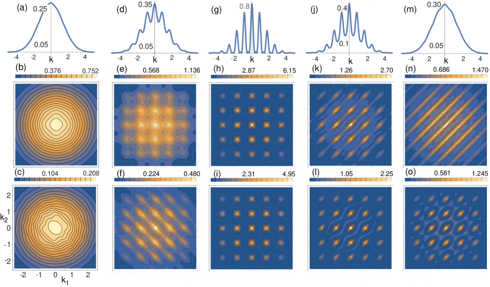
Figure 9: Momentum correlation plots and maps for the ground state of 3 bosons in 3 wells. Top row (a,d,g,j,m): 1st-order correlations ${}^{1}{\cal G}_{i}^{b}(k)$ (vertical axes) in units of $\mu$m. Middle row (b,e,h,k,n): 2nd-order correlations ${}^{2}{\cal G}_{i}^{b}(k_{1},k_{2})$ in units of $\mu$m² according to the color bars on top of each panel. Bottom row (c,f,i,l,o): 3rd-order (cuts at $k_{3}=0$) correlations ${}^{3}{\cal G}_{i}^{b}(k_{1},k_{2},k_{3}=0)$ in units of $\mu$m³ according to the color bars on top of each panel. The momenta $k$, $k_{1}$, and $k_{2}$ are in units of 1/$\mu$m. From left to right column: ${\cal U}=-200$, $-10$, $0$, $10$, and $300$ [see Eqs. (51) and (46) with $i=1$, as well as Eqs. (37) and (44) with $i=1$]. The choice of parameters is: interwell distance $d=7$ $\mu$m and spectral width of single-particle distribution in momentum space [see Eq. (35)] being the inverse of $s=0.35$ $\mu$m. The value of the plotted correlation functions in the bottom two rows was multiplied by a factor of 10 to achieve better contrast for the map features.

IX Signatures of emergent quantum phase transitions

The system of 3 bosons in 3 wells is a building block of bulk-size systems containing a large number of bosons (e.g., ⁸⁷Rb or ⁴He^∗ atoms) in 3D, 2D, and 1D optical lattices. Such bulk-like systems have been available already for some time and several physical aspects of them have been explored experimentally grei02 ; gerb05 ; gerb05.2 ; clem18 ; clem19 ; bloc05 , accompanied by theoretical studies seng05 ; triv09 . In particular, of direct interest to this paper are the observations, obtained through time-of-flight measurements, of the superfluid to Mott insulator phase transition grei02 ; gerb05 ; gerb05.2 ; clem18 ; clem19 (in 3D lattices), and of the second-order particle interference bloc05 (in 1D lattices) in analogy with a quantal extension of Hanburry Brown-Twiss-type optical interference.

The detailed algebraic analysis of all-order correlations presented earlier for the system of 3 bosons in 3 wells provides the tools for exploring these major physical aspects (quantum phase transitions and quantum-optics analogies) in the context of a finite-size system. In this respect, it is a first step towards the deciphering of the evolution of these aspects as the system size increases from a few particles to the thermodynamic limit. In this section, we analyze the signatures for quantum phase transitions that appear already in the case of a finite system as small as 3 bosons.

We begin by collecting in a single figure (Fig. 9) and for the ground state of the 3 bosons-3 wells systems all three levels of correlations as a function of the interaction strength ${\cal U}$ (with ${\cal U}=-200$, $-10$, 0, 10, and 300). For large ${\cal U}$ (${\cal U}=300$, describing very strong repulsive interparticle interaction), the system’s ground-state Hubbard eigenvector is very close to the single ket No. 1 $\rightarrow|111\rangle$ [see $\phi_{1}^{b,+\infty}$ in Eq. (14)] which describes exclusively singly-occupied sites. For 3 bosons in 3 wells, the state $|111\rangle$ is the analog of the Mott insulator phase, familiar from bulk systems. The associated three-body wave function is well approximated by the permanent $\Phi^{b,+\infty}_{1}(k_{1},k_{2},k_{3})$ [see Eq. (38)] formed from the three localized orbitals $\psi_{j}(k)$ in Eq. (35).

A crucial observation is that the corresponding single-particle momentum density (first-order correlation) portrayed in frame (m) of Fig. 9 (in top row) is structureless and devoid of any oscillatory pattern, in contrast to fully developed oscillations present in the single-particle density of the non-interacting ground state [see frame (g) in top row of Fig. 9]. As was the case with the bulk systems, this structureless pattern in the first-order correlation can thus be used as a signature of the Mott insulator even in the case of a small system.

In analogy with the interpretation for bulk systems, the appearance of oscillations in the non-interacting case can be associated with the spreading of the single-particle orbitals over all the three sites (three wells). Namely, for ${\cal U}=0$, the lowest energy single-particle wave function of the tight-binding Hamiltonian (in matrix representation)

$$H_{b,{\rm TB}}^{\rm sp}=-J\left(\begin{array}[]{ccc}0&1&0\\ 1&0&1\\ 0&1&0\\ \end{array}\right)$$ (61)

is a molecular orbital which is expressed as a coherent linear superposition of all three localized atomic orbitals $\psi_{j}(k)$ [with $j=1,2,3$, see Eq. (35)], namely

$$\begin{split}\psi_{\rm MO}(k)&=\frac{\psi_{1}(k)}{2}+\frac{\psi_{2}(k)}{\sqrt{2}}+\frac{\psi_{3}(k)}{2}\\ &=\frac{2^{1/4}\sqrt{s}}{\pi^{1/4}}e^{-k^{2}s^{2}}\left(\frac{e^{-idk}}{2}+\frac{1}{\sqrt{2}}+\frac{e^{idk}}{2}\right).\end{split}$$ (62)

Then the three-body wave function is constructed by triply occupying this molecular orbital, i.e., it is given by the Bose-Einstein-condensate product

$$\Phi^{b,{\cal U}=0}_{1}(k_{1},k_{2},k_{3})=\psi_{\rm MO}(k_{1})\psi_{\rm MO}(k_{2})\psi_{\rm MO}(k_{3}).$$ (63)

Eq. (63) above equals expression (41) derived by us earlier (see Sec. V) as the ${\cal U}=0$ limit of the solution of the Bose-Hubbard Hamiltonian [Eq. (2)], obtained through the matrix representation [Eq. (3)] in the 10-ket basis [Eq. (1)] for the problem of three bosons trapped in three-wells.

Because of the molecular orbital in Eq. (62), which expresses the delocalization of the single-particle wave functions over the whole system, the three-body wave function $\Phi^{b,{\cal U}=0}_{1}(k_{1},k_{2},k_{3})$ can be characterized as describing a superfluid phase in analogy with the bulk case grei02 ; fish89 . The natural difference of course is that in the bulk case the superfluid to Mott-insulator transition happens abruptly at ${\cal U}=z\times 5.8$ fish89 , with $z$ being the number of next neighbors of a lattice site, whereas for the small finite system this transition is not sharp but proceeds continuously as a function of ${\cal U}$. Some steps of this smooth evolution are illustrated in frame (g) (${\cal U}=0$), frame (j) (${\cal U}=10$), and frame (m) (${\cal U}=300$) of Fig. 9 (top row).

Furthermore, another aspect from the bulk studies that is relevant to our 3-boson results is the determination, made deeply in the Mott-insulator region, of a small oscillatory contribution to the single-particle density superimposed on the structureless background gerb05 ; gerb05.2 ; seng05 ; triv09 . This contribution note1 was found to vary as $\propto-2\sum_{\nu=x,y,z}\cos(k_{\nu}d)/{\cal U}$, as obtained via perturbative (or related) approaches around ${\cal U}\rightarrow+\infty$. Our exact algebraic expression for ${}^{1}{\cal G}_{i}^{b}(k)$ [Eq. (51)], which is valid for any ${\cal U}$, contains a second term $\cos(2dk)$ in addition to the $\cos(dk)$ term. Deeply in the Mott-insulator regime, however, there is agreement at the qualitative level between our result and the bulk one, because the coefficient ${\cal A}^{1}_{2}$ vanishes much faster than the coefficient ${\cal A}^{1}_{1}$ as ${\cal U}\rightarrow+\infty$ as is revealed by an inspection of the curves in frame (a) of Fig. 7.

At the non-interacting limit (${\cal U}=0$), however, this second term cannot be neglected [see frame (a) in Fig. 7 and Eq. (53)]. In this limit, its effect is to narrow the width of the cosinusoidal peaks at $k=2\pi j/d$, with $j=0,1,2,\ldots$. From this, one can conjecture yannun that for larger systems with $N$ bosons, all cosine terms of the form $\cos(ndk)$ with $n=1,2,3,\ldots,N-1$ (corresponding to all possible interwell distances) will contribute. The summation of many of such terms will enhance further the shrinking of the width of the main peaks, while it will give a practically vanishing result in the in-between regions. Thus the main peaks will acquire the shape of sharp spikes as was indeed observed grei02 in the bulk systems.

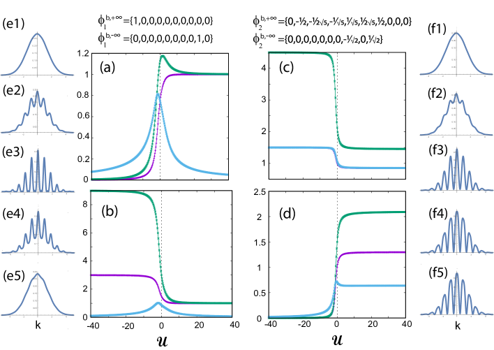
Figure 10: (a,b,c,d) Site occupations (vertical axes, dimensionless) and their fluctuations (vertical axes, dimensionless) for the ground, $\phi_{1}^{b}({\cal U})$ (a,b), and first-excited, $\phi_{2}^{b}({\cal U})$ (c,d), states as a function of the strength ${\cal U}$ of the interaction. Panels (a) and (c) refer to the left site (well), whereas panels (b) and (d) refer to the middle site (well). Violet color (midle curve at ${\cal U}=+40$): site occupations. Green color (upper curve at ${\cal U}=+40$): expectation value of the square of the site number operator. Light blue color (lower curve at ${\cal U}=+40$): standard deviation. Note that the middle and lower curves in frame (c) coincide for all practical purposes. (ex,fx) The first-order correlations for the ground and first-excited states, respectively, for five characteristic values : ${\cal U}=-200$ (x=1) (close to $\rightarrow-\infty$), -10 (x=2), 0 (x=3), 10 (x=4), and 300 (x=5) (close to $\rightarrow+\infty$). The first-order correlations ${}^{1}{\cal G}^{b}(k)$ (vertical axes) are in units of $\mu$m and the momenta $k$ are in units of 1/$\mu$m. The choice of parameters for the correlations is: interwell distance $d=7$ $\mu$m and spectral width of single-particle distribution in momentum space [see Eq. (35)] being the inverse of $s=0.35$ $\mu$m.

In the present paper, we cover the full range of interaction strengths, from infinite attraction (${\cal U}\rightarrow-\infty$) to infinite repulsion (${\cal U}\rightarrow+\infty$). Following the sequence of frames from the third to the first frame in Fig. 9 (top row), it is seen that a structureless single-particle momentum density emerges also in the limit ${\cal U}\rightarrow-\infty$; for intermediate negative values of ${\cal U}$, the weight of the oscillatory pattern decreases gradually as the absolute value $|{\cal U}|$ increases. However, based on our full solution of the 3 bosons-3 wells Hubbard system, it is apparent that this succession (i.e., from the third to the first frame of Fig. 9) does not reflect a transition from a superfluid to a Mott-insulator phase. Indeed, the Hubbard ground-state eigenvector for ${\cal U}\rightarrow-\infty$ is given by $\phi_{1}^{b,-\infty}$ in the second line of Eq. (14), which can properly be characterized as a Bose-Einstein condensate; namely, this ground state consists only of a single basis ket (No. 9 $\rightarrow|030\rangle$) that represents a triply occupied atomic orbital $\psi_{2}(k)$ [see Eq. (35)] located in the middle well.

The caveat from the discussion above is that the first-order correlation does not uniquely characterize the associated many-body state. This is not an uncommon occurrence, as can be also seen from an inspection of Fig. 8, which illustrates a succession of ${}^{1}{\cal G}_{2}^{b}(k)$’s for the first excited state. Indeed, the single-particle momentum density in frame (a) in Fig. 8 (case of ${\cal U}=-200$) is structureless; however, the corresponding Hubbard eigenvector is very well approximated by $\phi_{2}^{b,-\infty}$ in the second line of Eq. (15). Naturally, this eigenvector represents a many-body state that is neither a Mott insulator nor a Bose-Einstein condensate. Rather it represents a $(-|300\rangle+|003\rangle)\sqrt{2}$ NOON state; the family of NOON states are a focal point in quantum-optics investigations oubook ; shihbook .

For a complete characterization of the many-body state under consideration, additional information, beyond the first-order correlations, is needed. A natural candidate to this effect are the maps for the second-order (Sec. VII) and third-order (Sec. VI) correlations investigated earlier. For example, in the case of the structureless single-particle momentum density cases discussed above [i.e., frame (m) in Fig. 9 (top row), frame (a) in Fig. 9 (top row), and frame (a) in Fig. 8], all three corresponding third-order correlation maps are drastically different [compare frame (c) in Fig. 9 (bottom row), frame (o) in Fig. 9 (bottom row), and frame (a) in Fig. 4].

Note that the information provided by second-order correlation maps only is still not sufficient for the full characterization of the underlying many-body state. Indeed, the second-order correlation maps in frame (b) of Fig. 9 (second row) (case of the ground state at ${\cal U}=-200$) is very similar to that in frame (a) of Fig. 6 (case of the first-excited state at ${\cal U}=-200$).

We stress again at this point that Figs. 4, 6, 8, and Fig. 9 illustrate graphically the ability of our methodology to determine all three levels of momentum correlations and their evolution as a function of the interaction strength ${\cal U}$, from the attractive to the repulsive regime, and thus to provide the tools for a complete characterization of the underlying many-body states.

Before leaving this section, we found it worthwhile to explicitly investigate the conjecture that vanishing fluctuations in the site occupations are always associated with a structureless first-order momentum correlation. To this effect, we plot in Fig. 10 the site occupation, $\langle\phi^{b}_{j}({\cal U})|n_{i}|\phi^{b}_{j}({\cal U})\rangle$ [the site number operator $n_{i}=\hat{b}^{\dagger}_{i}\hat{b}_{i}$; see below Eq. (2)], the expectation value of the square of the site number operator, $\langle\phi^{b}_{j}({\cal U})|n_{i}^{2}|\phi^{b}_{j}({\cal U})\rangle$, and the standard deviation, $\sqrt{\langle\phi^{b}_{j}({\cal U})|n_{i}^{2}|\phi^{b}_{j}({\cal U})\rangle-\langle\phi^{b}_{j}({\cal U})|n_{i}|\phi^{b}_{j}({\cal U})\rangle^{2}}$ for the ground ($j=1$) and first-excited ($j=2$) states and for the left $(i=1)$ and middle ($i=2$) sites (wells). As already noted in the introductory section of this paper, the connection between the fluctuations in site-occupation and the appearance of structural patterns (or the lack thereof) in the first-order momentum correlations is a manifestation of the connection between the quantum phase-transition from superfluid (coherent) to localized (incoherent) states, and the quantum uncertainty relation connecting the fluctuations in phase and number (site-occupancy).

From an inspection of the four panels (a,b,c,d) in Fig. 10, one concludes that indeed in all four panels an oscillatory pattern in the single-particle momentum density [see subpanels (e2,e3,e4) and (f2,f3,f4,f5)] is accompanied by a nonvanishing fluctuation in the site occupations. However, a structureless single-particle momentum density is not always associated with a vanishing fluctuation; see the case of the NOON state $\phi^{b,-\infty}_{2}$ [Fig. 10(c)] for which the standard deviation of the left well is 3/2, whereas the corresponding single-particle momentum density [Fig. 10(f1)] is structureless.

Finally, we mention that temperature effects on the quantum phase transitions in bosonic gases trapped in optical lattices have recently attracted some attention (see, e.g., Refs. lu06 ; jin19 ). Our beyond-mean-field theoretical approach can be generalized yannun to account for such effects, but this falls outside the scope of the present paper.

X Analogies with three-photon interference in quantum optics

In this section, we elaborate on the analogies between our results for the system of 3 massive bosons trapped in 3 wells with the three-photon interference in quantum optics, which is an area of frontline research activities spag13 ; tich14 ; agar15 ; agne17 ; mens17 ; tamm18.1 ; tamm18.2 ; tamm19 . Such three-photon interference investigations fall into two major categories: (1) Those that employ a tritter note2 to produce a scattering event between three photons impinging on the input ports of a tritter and which measure coincidence probabilities for the photons exiting the three output ports spag13 ; tich14 ; agar15 ; agne17 ; mens17 . At the abstract theoretical level, the scattering event is described by a unitary scattering matrix. The coincidence probabilities are denoted as $P_{111}$ (one photon in each one of the output ports), $P_{210}$ (two photons in the first port and a single photon in the second port), $P_{300}$ (three photons in the first port), etc…, and they are apparently a direct generalization of the $P_{11}$ and $P_{20}$ coincidence probabilities familiar from the celebrated HOM hom87 two-photon interference experiment. Variations in the $P_{ijk}$, with $i,j,k=0,1,2,3$ and $i+j+k=3$, probabilities are achieved through control of the time delays between photons and other parameters of the tritter. (2) Those that resolve the intrinsic conjugate variables underlying the wave packets of the impinging photons on the tritter (i.e., frequency, $\omega$, and time delay, $\tau$) tamm18.1 ; tamm18.2 ; tamm19 ; for earlier two-photon interference investigations in this category, see Refs. lege04 ; gerr15.1 ; gerr15.2 . This category of experiments produces spectral correlation landscapes as a function of the three frequencies $\omega_{1}$, $\omega_{2}$, and $\omega_{3}$.

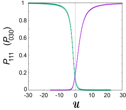
Figure 11: The (dimensionless) Hong-Ou-Mandel-type probabilities $P_{111}$ (violet, right curve) and $P_{030}$ (green, left curve) associated with the Hubbard ground-state vector $\phi^{b}_{1}({\cal U})$ as a function of the interaction strength ${\cal U}$ (dimensionless).

In the case of the 3 bosons in 3 wells, the quantum-optics category (1) above finds an analog to in situ experiments and their theoretical treatments. Indeed, the analogs of the three-photon wave function in the output ports are the vector solutions [stationary or time-dependent (not considered in this paper)] of the Hubbard Hamiltonian matrix in Eq. (3); compare the general form of the Hubbard vector solutions [Eq. (12) in Sec. II] to Eq. (5) for the three-photon output state from a tritter in Ref. agar15 . Control of these Hubbard vector solutions is achieved through variation of the interaction parameter ${\cal U}$ and the choice of a ground or excited state. For example, choosing the ground-state vector, the probability for finding only one boson in each well is given by the modulus square of the ${\cal U}$-dependent coefficient in the Hubbard eigenvector [Eq. (12)] in front of the basis ket No. 1 $\rightarrow|111\rangle$, i.e., $P_{111}({\cal U})=|{\bf c}_{111}({\cal U})|^{2}$; naturally $P_{030}({\cal U})=|{\bf c}_{030}({\cal U})|^{2}$.

In Fig. 11, we plot the $P_{111}({\cal U})$ and $P_{030}({\cal U})$ probabilities associated with the Hubbard ground-state eigenvector $\phi^{b}_{1}({\cal U})$. This figure is reminiscent of Fig. 2 in Ref. spag13 (see also Fig. 3 in Ref. agar15 ). It is interesting to note that the three-photon state $\ket{300}$ (experimentally realized in Ref. spag13 ) is described in quantum optics as a “three-photon bosonic coalescence”, whereas for atomic and molecular physics a description as a micro Bose-Einstein condensate appears to come naturally in mind.

Note, further, that the $P_{ijk}$’s in Ref. spag13 depend on two parameters, instead of a single one. For the case of 3 massive bosons in 3 wells, a second parameter becomes relevant by considering the time evolution of the Hubbard vector solutions yannun ; see Refs. yann19.1 ; kauf14 for the consideration of the time-evolution in the case of 2 massive bosons in 2 wells. Note further that, in quantum optics, two fully overlapping photons are described as perfectly indistinguishable, whereas two non-overlapping photons are described as perfectly distinguishable spag13 ; tich14 . In the context of the present study for 3 massive trapped bosons (which uses the assumption $d^{2}/s^{2}>>1$), an example of the former is the ket No. 9 $\rightarrow|030\rangle$, whereas an example of the latter is the ket No. 1 $\rightarrow|111\rangle$. A double-single occupancy ket, like ket No. 2 $\rightarrow|210\rangle$, can be referred to as a mode with two indistinguishable and one distinguishable bosons tich14 .

The analogy between the two-photon optical HOM formalism and the vector solutions of the Hubbard theoretical modeling for 2 bosons (or 2 fermions) in 2 wells was reported earlier in Refs. bran18 ; yann19.1

Furthermore, in the case of the 3 bosons in 3 wells, the quantum-optics category (2) above finds an analog to time-of-flight experiments and their theoretical treatments. This analogy derives from the following correspondence (revealed in Ref. yann19.1 )

$$\begin{split}k&\longleftrightarrow\omega/c\\ d&\longleftrightarrow\tau c\\ kd&\longleftrightarrow\omega\tau.\end{split}$$ (64)

As was done yann19.1 for the case of 2 massive trapped particles versus two interfering photons, this correspondence can be used to establish a complete analogy between the cosinusoidal patterns of all three orders of momentum correlation functions presented in this paper for 3 massive and trapped bosons (and which can be determined experimentally through time-of-flight measurements prei19 ) with the landscapes tamm18.1 ; tamm19 of the frequency-resolved three-photon interferograms (which are a function of the three photon frequencies, $\omega_{1}$, $\omega_{2}$, and $\omega_{3}$). For example the interferograms in Fig. 3 of Ref. tamm19 are analogous to the map in Fig. 9 [frame (i), bottom row] of the $k_{3}=0$ cut of the third-order momentum correlation associated with 3 non-interacting trapped massive bosons. A difference to keep in mind is that in this paper the interwell distances were taken to be equal, whereas the time delays in Ref. tamm19 are unequal.

Furthermore, Eq. (S1) in the Supplemental Material of Ref. tamm19 which describes the three-photon output wave function at the detectors, $\psi(\omega_{1},\omega_{2},\omega_{3})$, is a permanent of the three single-photon wave functions $\chi_{j}(\omega_{i})=E_{j}(\omega_{i})\exp(-i\omega_{i}t_{j})$, with $i,j=1,2,3$, where $t_{j}$ denotes time instances [corresponding to the position of each well in our single-particle orbitals displayed in Eq. (35)]. As a result, for $E_{1}(\omega_{i})=E_{2}(\omega_{i})=E_{2}(\omega_{i})=E(\omega_{i})$ and $t_{1}=-\tau$, $t_{2}=0$, and $t_{3}=\tau$, it reduces exactly to the form of the three-body wave function $\Phi^{b,+\infty}_{1}(k_{1},k_{2},k_{3})$ [see top line in Eq. (38)] in this paper which is associated with the case of the three singly-occupied wells, i.e., the Hubbard solution at infinite repulsion, $|111\rangle$ (perfectly distinguishable bosons).

A central focus in the recent quantum-optics literature has been the demonstration of genuine three-photon interference agne17 ; mens17 , that is interference effects that cannot be inferred by a knowledge of the one- and two-photon interference patterns. In the language of many-body literature for massive particles, this is equivalent to isolating the connected terms, ${\cal G}_{\rm con}$, in the total third-order correlations by subtracting the disconnected ones, ${\cal G}_{\rm dis}$. Reflecting its name, the disconnected contribution to the total third-order correlation consists of products of the first- and second-order correlations.

For the case of 3 perfectly distinguishable bosons in 3 wells (described by the ket $|111\rangle$), one can observe that the first-order momentum correlation given in Eqs. (54) and (52) does not contain any cosine (or sine) terms, whereas the second-order momentum correlation given in Eq. (48) contains consine terms with two momenta in the cosine arguments. As a result, the connected part of the third-order momentum correlations [see Eq. (40)] is necessarily reflected in the cosine terms having an argument that depends on all three single-particle momenta $k_{1}$, $k_{2}$, and $k_{3}$. Another way to view the above remarks is that the genuine three-body interference involves a total phase $\varphi$ which is the sum of three partial phases $\varphi_{1}$, $\varphi_{2}$, and $\varphi_{3}$, associated with the individual bosons, i.e., $\varphi=\varphi_{1}+\varphi_{2}+\varphi_{3}$. Such a triple phase (referred to also as a triad phase) has been prominent in the quantum-optics literature agne17 ; mens17 regarding genuine three-photon interference.

Specifically, the disconnected part of the third-order correlation for 3 bosons is given by the expression

$$\begin{split}&{}^{3}{\cal G}_{\rm dis}^{b}(k_{1},k_{2},k_{3})=-2{{}^{1}{\cal G}^{b}(k_{1})}{{}^{1}{\cal G}^{b}(k_{2})}{{}^{1}{\cal G}^{b}(k_{3})}+\\ &{{}^{1}{\cal G}^{b}(k_{1})}{{}^{2}{\cal G}^{b}(k_{2},k_{3})}+{{}^{1}{\cal G}^{b}(k_{2})}{{}^{2}{\cal G}^{b}(k_{1},k_{3})}+\\ &{{}^{1}{\cal G}^{b}(k_{3})}{{}^{2}{\cal G}^{b}(k_{1},k_{2})}.\end{split}$$ (65)

We can apply the above expression immediately to the case of the Hubbard ground-state eigenvector $\ket{111}$ (limit of infinite repulsion, 3 perfectly distinguishable bosons), because we have derived explicit algebraic expressions for the corresponding third-order [Eq. (40)], second-order [Eq. (48)], and first-order momentum correlations [Eqs. (54) and (52)]. Indeed one finds for the connected correlation part

$$\begin{split}&{}^{3}{\cal G}_{1,\rm con}^{b,+\infty}(k_{1},k_{2},k_{3})=\\ &{}^{3}{\cal G}_{1}^{b,+\infty}(k_{1},k_{2},k_{3})-^{3}{\cal G}_{1,\rm dis}^{b,+\infty}(k_{1},k_{2},k_{3})=\\ &\frac{4\sqrt{2}}{3\pi^{3/2}}s^{3}e^{-2s^{2}(k_{1}^{2}+k_{2}^{2}+k_{3}^{2})}\big{\{}\cos(d(k_{1}+k_{2}-2k_{3}))\\ &+\cos(d(k_{2}+k_{3}-2k_{1}))+\cos(d(k_{1}+k_{3}-2k_{2}))\big{\}}.\end{split}$$ (66)

It is worth noting that the result in Eq. (66) above for the connected correlation part for 3 perfectly distinguishable bosons in 3 wells coincides with the corresponding result prei19 ; yann19.3 for 3 perfectly distinguishable fully spin polarized fermions in 3 wells.

XI Summary

In this paper, we develop and expand a formalism and a theoretical framework, which, with the use of an algebraic-language computations tool (MATHEMATICA math18 ), allows us to derive explicit analytic expressions for all three orders (third, second, and first) of momentum-space correlations for 3 interacting ultracold bosonic atoms confined in 3 optical wells in a linear geometry. This 3b-3w system was modeled as a three-site Bose-Hubbard Hamiltonian whose 10 eigenvectors were mapped onto first-quantization three-body wave functions in momentum space by: (1) associating the bosons with the Fourier transforms of displaced Gaussian functions centered on each well, and (2) constructing the permanents associated with the basis kets of the Hubbard Hilbert space by using the Fourier transforms of the displaced Gaussians describing the trapped bosons. The 3rd-order momentum-space correlations are the modulus square of such three-body wave functions, and the second- and first-order correlations are derived through successive integrations over the unresolved momentum variables. This methodology applies to all bosonic states with strong note4 or without entanglement, and does not rely on the standard Wick’s factorization scheme, employed in earlier studies (see, e.g., Refs, gome06 ; hodg13 ; schm17 ) of higher-order momentum correlations for expanding or colliding Bose-Einstein condensates of ultracold atoms.

The availability of such explicit analytic correlation functions will greatly assist in the analysis of anticipated future TOF measurements with few ($N>2$) ultracold atoms trapped in optical lattices, following the demonstrated feasibility of determining higher-than-first-order momentum correlation functions via single-particle detection in the case of $N=2$ fermionic ⁶Li atoms berg19 , $N=3$ fully spin-polarized fermionic ⁶Li atoms prei19 , and a large number of bosonic ⁴He^∗ atoms clem19 .

The availability of the complete set of all-order momentum correlations enabled us to reveal and explore in detail two major physical aspects of the 3b-3w ultracold-atom system: (I) That a small system of only 3 bosons exhibits indeed an embryonic behavior akin to an emergent superfluid to Mott transition and (II) That both the in situ and TOF spectroscopies of the 3b-3w system exhibit analogies with the quantum-optics three-photon interference, including the aspects of genuine three-photon interference which cannot be understood from the knowledge of the lower second- and first-order correlations alone agne17 ; mens17 .

The superfluid to Mott-insulator transition in extended optical lattices grei02 ; gerb05 ; gerb05.2 was explored based on the variations in the shape of the first-order momentum correlations. For the 3b-3w system, we reported clear variations of the first-order momentum correlations, from being oscillatory with a period that depends on the inter-well distance, characteristic of a coherent state of a superfluid phase with multiple site occupancies by each of the trapped ultracold bosonic atoms (high site-occupancy uncertainty), to a structureless shape characteristic of localized states, (see below) with low site-occupancy uncertainty and consequent high phase-uncertainty (incoherent phase). Furthermore, we also concluded that the first-order momentum correlations are not sufficient to characterize uniquely the underlying nature of a state of the 3b-3w system. To this effect, knowledge of all three orders of correlations is needed. Indeed, a structureless first-order correlation relates to three different 3b-3w states, i.e., the $|030\rangle$ ground state at ${\cal U}\rightarrow-\infty$ (Bose-Einstein condensate), the $|111\rangle$ ground state at ${\cal U}\rightarrow+\infty$ (Mott insulator), and the $(-|300\rangle+|003\rangle)/\sqrt{2}$ first-excited state at ${\cal U}\rightarrow-\infty$ (NOON state).

Concerning the quantum optics analogies, we established that in situ measurements of the site occupation probabilities as a function of ${\cal U}$, $P_{ijk}({\cal U})$ (with $i,j=1,\ldots,3$), provide analogs of the celebrated HOM coincidence probabilities for three photons at the output ports of a tritter as discussed in Refs. spag13 ; agar15 . We further established that the momentum-space all-order correlations for the 3b-3w system parallel the frequency-resolved interferograms of distinguishable photons as explored in Refs. tamm18.1 ; tamm18.2 ; tamm19 . The analogies with the genuine three-photon interference were established in the framework of the many-body theoretical concepts of disconnected versus connected correlation terms.

To achieve simplicity in this paper, we assumed throughout that the interwell separation is much larger than the width of the single-particle Gaussian function in the real configuration space, i.e., $d^{2}/s^{2}>>1$ (see Sec. IV). This is equivalent to considering localized bosons with vanishing overlaps (distinguishable bosons in different wells) or unity overlaps (indistinguishable bosons in the same well); indeed the overlap of two single-particle wave functions according to Eq. (35) is given by $S=e^{-d^{2}/(8s^{2})}$. Considering cases with small, but finite $S$, which represent partial indistinguishability tich14 , complicates substantially the analytic results yannun .

Finally, we note here that our all-order momentum-space correlations for the 3b-3w system can contribute an alternative way to study and explore with massive particles aspects of the boson sampling problem aaar13 , and in particular its extension to the multiboson correlation sampling tamm15 ; tamm15.1 . We note that boson sampling problems have become a major focus [see, e.g., Refs. tamm15 ; tamm15.1 ; tich14 ; lain14 ; wals19 ] in quantum-optics investigations because they are considered to be an intermediate step on the road towards the implementation of the quantum computer.

XII Acknowledgments

This work has been supported by a grant from the Air Force Office of Scientific Research (AFOSR, USA) under Award No. FA9550-15-1-0519. Calculations were carried out at the GATECH Center for Computational Materials Science.

Appendix A Hubbard eigenvectors: The infinite repulsive or attractive interaction (${\cal U}\rightarrow\pm\infty$) limit for the remaining eight excited states

This Appendix complements Sec. II.1 by listing without commentary the Hubbard eigenvectors of the remaining eight excited states not discussed in the main text.

$$\begin{split}\phi^{b,+\infty}_{3}&=\left\{0,\frac{1}{2},\frac{1}{2\sqrt{5}},\frac{1}{\sqrt{5}},\frac{1}{\sqrt{5}},\frac{1}{2\sqrt{5}},\frac{1}{2},0,0,0\right\}\\ \phi^{b,-\infty}_{3}&=\{0,0,0,0,0,0,0,\frac{1}{\sqrt{2}},0,\frac{1}{\sqrt{2}}\}\end{split}$$ (67)

$$\begin{split}\phi^{b,+\infty}_{4}&=\left\{0,0,\sqrt{\frac{2}{5}},-\frac{1}{\sqrt{10}},-\frac{1}{\sqrt{10}},\sqrt{\frac{2}{5}},0,0,0,0\right\}\\ \phi^{b,-\infty}_{4}&=\left\{0,-\frac{1}{2},-\frac{1}{2\sqrt{5}},-\frac{1}{\sqrt{5}},-\frac{1}{\sqrt{5}},-\frac{1}{2\sqrt{5}},-\frac{1}{2},0,0,0\right\}\end{split}$$ (68)

$$\begin{split}\phi^{b,+\infty}_{5}&=\left\{0,0,-\sqrt{\frac{2}{5}},\frac{1}{\sqrt{10}},-\frac{1}{\sqrt{10}},\sqrt{\frac{2}{5}},0,0,0,0\right\}\\ \phi^{b,-\infty}_{5}&=\left\{0,\frac{1}{2},\frac{1}{2\sqrt{5}},\frac{1}{\sqrt{5}},-\frac{1}{\sqrt{5}},-\frac{1}{2\sqrt{5}},-\frac{1}{2},0,0,0\right\}\end{split}$$ (69)

$$\begin{split}\phi^{b,+\infty}_{6}&=\left\{0,-\frac{1}{2},\frac{1}{2\sqrt{5}},\frac{1}{\sqrt{5}},-\frac{1}{\sqrt{5}},-\frac{1}{2\sqrt{5}},\frac{1}{2},0,0,0\right\}\\ \phi^{b,-\infty}_{6}&=\left\{0,0,-\sqrt{\frac{2}{5}},\frac{1}{\sqrt{10}},-\frac{1}{\sqrt{10}},\sqrt{\frac{2}{5}},0,0,0,0\right\}\end{split}$$ (70)

$$\begin{split}\phi^{b,+\infty}_{7}&=\left\{0,\frac{1}{2},-\frac{1}{2\sqrt{5}},-\frac{1}{\sqrt{5}},-\frac{1}{\sqrt{5}},-\frac{1}{2\sqrt{5}},\frac{1}{2},0,0,0\right\}\\ \phi^{b,-\infty}_{7}&=\left\{0,0,\sqrt{\frac{2}{5}},-\frac{1}{\sqrt{10}},-\frac{1}{\sqrt{10}},\sqrt{\frac{2}{5}},0,0,0,0\right\}\end{split}$$ (71)

$$\begin{split}\phi^{b,+\infty}_{8}&=\left\{0,0,0,0,0,0,0,\frac{1}{\sqrt{2}},0,\frac{1}{\sqrt{2}}\right\}\\ \phi^{b,-\infty}_{8}&=\left\{0,-\frac{1}{2},\frac{1}{2\sqrt{5}},\frac{1}{\sqrt{5}},\frac{1}{\sqrt{5}},\frac{1}{2\sqrt{5}},-\frac{1}{2},0,0,0\right\}\end{split}$$ (72)

$$\begin{split}\phi^{b,+\infty}_{9}&=\left\{0,0,0,0,0,0,0,-\frac{1}{\sqrt{2}},0,\frac{1}{\sqrt{2}}\right\}\\ \phi^{b,-\infty}_{9}&=\left\{0,\frac{1}{2},-\frac{1}{2\sqrt{5}},-\frac{1}{\sqrt{5}},\frac{1}{\sqrt{5}},\frac{1}{2\sqrt{5}},-\frac{1}{2},0,0,0\right\}\\ \end{split}$$ (73)

$$\begin{split}\phi^{b,+\infty}_{10}&=\{0,0,0,0,0,0,0,0,1,0\}\\ \phi^{b,-\infty}_{10}&=\{-1,0,0,0,0,0,0,0,0,0\}\end{split}$$ (74)

Appendix B Hubbard eigenvectors: The noninteracting (${\cal U}=0$) limit for the remaining eight excited states

Because of the three pairwise degeneracies [see Eq. (27)], care must be used when determining the six eigenvectors 3, 4, 5, 6, 7, and 8 at ${\cal U}=0$. The proper Hubbard eigenvectors listed below were determined by taking the limit ${\cal U}\rightarrow 0+$. For the eigenvectors No. 3, 4, 7, and 8, the associated algebraic formulas are lengthy, and as a result we give below the numerical expressions of these eigenvectors. Eigenvector No. 5 is ${\cal U}$-independent.

$$\begin{split}&\phi_{3r(4l)}^{b,{\cal U}=0}=\\ &\{-0.553362,0.189903,-0.419079,0.142399,0.142399,\\ &-0.419079,0.189903,0.232583,0.348804,0.232583\},\end{split}$$ (75)

$$\begin{split}&\phi_{4r(3l)}^{b,{\cal U}=0}=\\ &\{-0.079316,0.346679,0.165823,-0.205481,-0.205481,\\ &0.165823,0.346679,0.424594,-0.503325,0.424594\},\end{split}$$ (76)

$$\begin{split}&\phi_{5r(6l)}^{b,{\cal U}=0}=\phi_{5}^{b,+\infty}=\phi_{6}^{b,-\infty},\end{split}$$ (77)

$$\begin{split}&\phi_{6r(5l)}^{b,{\cal U}=0}=\\ &\left\{0,0,\frac{\sqrt{\frac{3}{5}}}{4},\frac{\sqrt{\frac{3}{5}}}{2},-\frac{\sqrt{\frac{3}{5}}}{2},-\frac{\sqrt{\frac{3}{5}}}{4},0,-\frac{\sqrt{5}}{4},0,\frac{\sqrt{5}}{4}\right\},\end{split}$$ (78)

$$\begin{split}&\phi_{7r(8l)}^{b,{\cal U}=0}=\\ &\{0.553362,-0.189903,-0.419079,0.142399,0.142399,\\ &-0.419079,-0.189903,0.232583,-0.348804,0.232583\},\end{split}$$ (79)

$$\begin{split}&\phi_{8r(7l)}^{b,{\cal U}=0}=\\ &\{0.079316,-0.346679,0.165823,-0.205481,-0.205481,\\ &0.165823,-0.346679,0.424594,0.503325,0.424594\},\end{split}$$ (80)

Finally, the remaining two eigenvectors No. 9 and No. 10 are given by,

$$\begin{split}&\phi_{9}^{b,{\cal U}=0}=\\ &\left\{0,\frac{1}{2},-\frac{1}{4\sqrt{2}},-\frac{1}{2\sqrt{2}},\frac{1}{2\sqrt{2}},\frac{1}{4\sqrt{2}},-\frac{1}{2},-\frac{\sqrt{\frac{3}{2}}}{4},0,\frac{\sqrt{\frac{3}{2}}}{4}\right\},\end{split}$$ (81)

and

$$\begin{split}&\phi_{10}^{b,{\cal U}=0}=\\ &\left\{-\frac{\sqrt{3}}{4},-\frac{\sqrt{\frac{3}{2}}}{4},\frac{\sqrt{3}}{8},\frac{\sqrt{3}}{4},\frac{\sqrt{3}}{4},\frac{\sqrt{3}}{8},-\frac{\sqrt{\frac{3}{2}}}{4},\frac{1}{8},-\frac{1}{2\sqrt{2}},\frac{1}{8}\right\}.\end{split}$$ (82)

Appendix C Third-order momentum correlations for 3 bosons in 3 wells: The infinite-interaction limit (${\cal U}\rightarrow\pm\infty$) for the remaining eight states

This Appendix complements Sec. IV by listing without commentary the momentum-space wave functions, $\Phi^{b,\pm\infty}_{i}(k_{1},k_{2},k_{3})$ (with $i=3,\ldots,10$), associated with the corresponding Hubbard eigenvectors, $\phi^{b,\pm\infty}_{i}$ [see Eqs. (67)-(74)], at the limits of infinite repulsive or attractive strength (i.e., for ${\cal U}\rightarrow\pm\infty$). The commentary integrating these wave functions into the broader scheme of their evolution as a function of any interaction strength $-\infty<{\cal U}<+\infty$ is left for Appendix E.

$$\begin{split}\Phi^{b,+\infty}_{3}(&k_{1},k_{2},k_{3})=\frac{2^{3/4}}{5\sqrt{3}\pi^{3/4}}s^{3/2}e^{-(k_{1}^{2}+k_{2}^{2}+k_{3}^{2})s^{2}}\\ &\times\left[\sqrt{5}\cos(d(-k_{1}+k_{2}+k_{3}))+\sqrt{5}\cos(d(k_{1}+k_{2}-k_{3}))\right.+\sqrt{5}\cos(d(k_{1}-k_{2}+k_{3}))\\ &\;\;+5\cos(d(k_{1}+k_{2}))+5\cos(d(k_{1}+k_{3}))+5\cos(d(k_{2}+k_{3}))+2\sqrt{5}\cos(dk_{1})\left.+2\sqrt{5}\cos(dk_{2})+2\sqrt{5}\cos(dk_{3})\right],\\ \Phi^{b,-\infty}_{3}(&k_{1},k_{2},k_{3})=\frac{2\times 2^{1/4}}{\pi^{3/4}}s^{3/2}e^{-(k_{1}^{2}+k_{2}^{2}+k_{3}^{2})s^{2}}\cos(d(k_{1}+k_{2}+k_{3})).\end{split}$$ (83)

$$\begin{split}\Phi^{b,+\infty}_{4}(&k_{1},k_{2},k_{3})=-\frac{2\times 2^{1/4}}{\sqrt{15}\pi^{3/4}}s^{3/2}e^{-(k_{1}^{2}+k_{2}^{2}+k_{3}^{2})s^{2}}\\ &\times\left[\cos(dk_{1})+\cos(dk_{2})+\cos(dk_{3})-2\cos(d(-k_{1}+k_{2}+k_{3}))-2\cos(d(k_{1}-k_{2}+k_{3})-2\cos(d(k_{1}+k_{2}-k_{3})]\right],\\ \Phi^{b,-\infty}_{4}(&k_{1},k_{2},k_{3})=-\frac{2^{3/4}}{5\sqrt{3}\pi^{3/4}}s^{3/2}e^{-(k_{1}^{2}+k_{2}^{2}+k_{3}^{2})s^{2}}\\ &\times\left[\sqrt{5}\cos(d(-k_{1}+k_{2}+k_{3}))+\sqrt{5}\cos(d(k_{1}+k_{2}-k_{3}))\right.+\sqrt{5}\cos(d(k_{1}-k_{2}+k_{3}))\\ &\;\;+5\cos(d(k_{1}+k_{2}))+5\cos(d(k_{1}+k_{3}))+5\cos(d(k_{2}+k_{3}))+2\sqrt{5}\cos(dk_{1})\left.+2\sqrt{5}\cos(dk_{2})+2\sqrt{5}\cos(dk_{3})\right].\end{split}$$ (84)

$$\begin{split}\Phi^{b,+\infty}_{5}(&k_{1},k_{2},k_{3})=-\frac{i2\times 2^{1/4}}{\sqrt{15}\pi^{3/4}}s^{3/2}e^{-(k_{1}^{2}+k_{2}^{2}+k_{3}^{2})s^{2}}\\ &\times\left[\sin(dk_{1})+\sin(dk_{2})+\sin(dk_{3})-2\sin(d(-k_{1}+k_{2}+k_{3}))-2\sin(d(k_{1}-k_{2}+k_{3}))-2\sin(d(k_{1}+k_{2}-k_{3}))\right],\\ \Phi^{b,-\infty}_{5}(&k_{1},k_{2},k_{3})=-\frac{i2^{3/4}}{5\sqrt{3}\pi^{3/4}}s^{3/2}e^{-(k_{1}^{2}+k_{2}^{2}+k_{3}^{2})s^{2}}\\ &\times\left[\sqrt{5}\sin(d(-k_{1}+k_{2}+k_{3}))+\sqrt{5}\sin(d(k_{1}+k_{2}-k_{3}))\right.+\sqrt{5}\sin(d(k_{1}-k_{2}+k_{3}))\\ &\;\;+5\sin(d(k_{1}+k_{2}))+5\sin(d(k_{1}+k_{3}))+5\sin(d(k_{2}+k_{3}))+2\sqrt{5}\sin(dk_{1})\left.+2\sqrt{5}\sin(dk_{2})+2\sqrt{5}\sin(dk_{3})\right].\end{split}$$ (85)

$$\begin{split}\Phi^{b,+\infty}_{6}(&k_{1},k_{2},k_{3})=-\frac{i2^{3/4}}{5\sqrt{3}\pi^{3/4}}s^{3/2}e^{-(k_{1}^{2}+k_{2}^{2}+k_{3}^{2})s^{2}}\\ &\times\left[\sqrt{5}\sin(d(-k_{1}+k_{2}+k_{3}))+\sqrt{5}\sin(d(k_{1}+k_{2}-k_{3}))\right.+\sqrt{5}\sin(d(k_{1}-k_{2}+k_{3}))\\ &\;\;-5\sin(d(k_{1}+k_{2}))-5\sin(d(k_{1}+k_{3}))-5\sin(d(k_{2}+k_{3}))+2\sqrt{5}\sin(dk_{1})\left.+2\sqrt{5}\sin(dk_{2})+2\sqrt{5}\sin(dk_{3})\right],\\ \Phi^{b,-\infty}_{6}(&k_{1},k_{2},k_{3})=-\frac{i2\times 2^{1/4}}{\sqrt{15}\pi^{3/4}}s^{3/2}e^{-(k_{1}^{2}+k_{2}^{2}+k_{3}^{2})s^{2}}\\ &\times\left[\sin(dk_{1})+\sin(dk_{2})+\sin(dk_{3})-2\sin(d(-k_{1}+k_{2}+k_{3}))-2\sin(d(k_{1}-k_{2}+k_{3}))-2\sin(d(k_{1}+k_{2}-k_{3}))\right].\end{split}$$ (86)

$$\begin{split}\Phi^{b,+\infty}_{7}(&k_{1},k_{2},k_{3})=-\frac{2^{3/4}}{5\sqrt{3}\pi^{3/4}}s^{3/2}e^{-(k_{1}^{2}+k_{2}^{2}+k_{3}^{2})s^{2}}\\ &\times\left[\sqrt{5}\cos(d(-k_{1}+k_{2}+k_{3}))+\sqrt{5}\cos(d(k_{1}+k_{2}-k_{3}))\right.+\sqrt{5}\cos(d(k_{1}-k_{2}+k_{3}))\\ &\;\;-5\cos(d(k_{1}+k_{2}))-5\cos(d(k_{1}+k_{3}))-5\cos(d(k_{2}+k_{3}))+2\sqrt{5}\cos(dk_{1})\left.+2\sqrt{5}\cos(dk_{2})+2\sqrt{5}\cos(dk_{3})\right],\\ \Phi^{b,-\infty}_{7}(&k_{1},k_{2},k_{3})=-\frac{2\times 2^{1/4}}{\sqrt{15}\pi^{3/4}}s^{3/2}e^{-(k_{1}^{2}+k_{2}^{2}+k_{3}^{2})s^{2}}\\ &\times\left[\cos(dk_{1})+\cos(dk_{2})+\cos(dk_{3})-2\cos(d(-k_{1}+k_{2}+k_{3}))-2\cos(d(k_{1}-k_{2}+k_{3}))-2\cos(d(k_{1}+k_{2}-k_{3}))\right].\end{split}$$ (87)

$$\begin{split}\Phi^{b,+\infty}_{8}(&k_{1},k_{2},k_{3})=\frac{2\times 2^{1/4}}{\pi^{3/4}}s^{3/2}e^{-(k_{1}^{2}+k_{2}^{2}+k_{3}^{2})s^{2}}\cos(d(k_{1}+k_{2}+k_{3})),\\ \Phi^{b,-\infty}_{8}(&k_{1},k_{2},k_{3})=\frac{2^{3/4}}{5\sqrt{3}\pi^{3/4}}s^{3/2}e^{-(k_{1}^{2}+k_{2}^{2}+k_{3}^{2})s^{2}}\\ &\times\left[\sqrt{5}\cos(d(-k_{1}+k_{2}+k_{3}))+\sqrt{5}\cos(d(k_{1}+k_{2}-k_{3}))\right.+\sqrt{5}\cos(d(k_{1}-k_{2}+k_{3}))\\ &\;\;-5\cos(d(k_{1}+k_{2}))-5\cos(d(k_{1}+k_{3}))-5\cos(d(k_{2}+k_{3}))+2\sqrt{5}\cos(dk_{1})\left.+2\sqrt{5}\cos(dk_{2})+2\sqrt{5}\cos(dk_{3})\right].\end{split}$$ (88)

$$\begin{split}\Phi^{b,+\infty}_{9}(&k_{1},k_{2},k_{3})=\frac{2i2^{1/4}}{\pi^{3/4}}s^{3/2}e^{-(k_{1}^{2}+k_{2}^{2}+k_{3}^{2})s^{2}}\sin(d(k_{1}+k_{2}+k_{3})),\\ \Phi^{b,-\infty}_{9}(&k_{1},k_{2},k_{3})=\frac{i2^{3/4}}{5\sqrt{3}\pi^{3/4}}s^{3/2}e^{-(k_{1}^{2}+k_{2}^{2}+k_{3}^{2})s^{2}}\\ &\times\left[\sqrt{5}\sin(d(-k_{1}+k_{2}+k_{3}))+\sqrt{5}\sin(d(k_{1}+k_{2}-k_{3}))\right.+\sqrt{5}\sin(d(k_{1}-k_{2}+k_{3}))\\ &\;\;-5\sin(d(k_{1}+k_{2}))-5\sin(d(k_{1}+k_{3}))-5\sin(d(k_{2}+k_{3}))+2\sqrt{5}\sin(dk_{1})\left.+2\sqrt{5}\sin(dk_{2})+2\sqrt{5}\sin(dk_{3})\right].\end{split}$$ (89)

$$\begin{split}\Phi^{b,+\infty}_{10}(&k_{1},k_{2},k_{3})=-\left(\frac{2}{\pi}\right)^{3/4}s^{3/2}e^{-(k_{1}^{2}+k_{2}^{2}+k_{3}^{2})s^{2}},\\ \Phi^{b,-\infty}_{10}(&k_{1},k_{2},k_{3})=-\frac{2\times 2^{1/4}}{\sqrt{3}\pi^{3/4}}s^{3/2}e^{-(k_{1}^{2}+k_{2}^{2}+k_{3}^{2})s^{2}}[\cos(d(k_{1}-k_{2}))+\cos(d(k_{1}-k_{3}))+\cos(d(k_{2}-k_{3}))].\end{split}$$ (90)

Appendix D Third-order momentum correlations for 3 bosons in 3 wells: The non-interacting limit ${\cal U}=0$ for the remaining eight states

This Appendix complements Sec. V by listing without commentary the momentum-space three-body wave functions for the remaining 8 excited states, that is:

$$\begin{split}&s^{-3/2}e^{(k_{1}^{2}+k_{2}^{2}+k_{3}^{2})s^{2}}\Phi_{3r(4l)}^{b,{\cal U}=0}(k_{1},k_{2},k_{3})=0.248595+0.117189\big{(}\cos(dk_{1})+\cos(dk_{2})+\cos(dk_{3})\big{)}\\ &-0.322013\big{(}\cos[d(k_{1}-k_{2})]+\cos[d(k_{1}-k_{3})]+\cos[d(k_{2}-k_{3})]\big{)}\\ &+0.156283\big{(}\cos[d(k_{1}+k_{2})]+\cos[d(k_{1}+k_{3})]+\cos[d(k_{2}+k_{3})]\big{)}\\ &-0.344886\big{(}\cos[d(k_{1}-k_{2}+k_{3})]+\cos[d(k_{1}-k_{2}-k_{3})]+\cos[d(k_{1}+k_{2}-k_{3})]\big{)}+0.331527\cos[d(k_{1}+k_{2}+k_{3})],\end{split}$$ (91)

$$\begin{split}&s^{-3/2}e^{(k_{1}^{2}+k_{2}^{2}+k_{3}^{2})s^{2}}\Phi_{4r(3l)}^{b,{\cal U}=0}(k_{1},k_{2},k_{3})=-0.358722-0.169103\big{(}\cos(dk_{1})+\cos(dk_{2})+\cos(dk_{3})\big{)}\\ &-0.0461557\big{(}\cos[d(k_{1}-k_{2})]+\cos[d(k_{1}-k_{3})]+\cos[d(k_{2}-k_{3})]\big{)}\\ &+0.285304\big{(}\cos[d(k_{1}+k_{2})]+\cos[d(k_{1}+k_{3})]+\cos[d(k_{2}+k_{3})]\big{)}\\ &+0.136466\big{(}\cos[d(k_{1}-k_{2}+k_{3})]+\cos[d(k_{1}-k_{2}-k_{3})]+\cos[d(k_{1}+k_{2}-k_{3})]\big{)}+0.605221\cos[d(k_{1}+k_{2}+k_{3})],\end{split}$$ (92)

$$\begin{split}\Phi_{5r(6l)}^{b,{\cal U}=0}(k_{1},k_{2},k_{3})=\Phi_{5}^{b,+\infty}(k_{1},k_{2},k_{3})=\Phi_{6}^{b,-\infty}(k_{1},k_{2},k_{3}),\end{split}$$ (93)

$$\begin{split}&\frac{-i2^{1/4}\sqrt{5}\pi^{3/4}}{s^{3/2}}e^{(k_{1}^{2}+k_{2}^{2}+k_{3}^{2})s^{2}}\Phi_{6r(5l)}^{b,{\cal U}=0}(k_{1},k_{2},k_{3})=2\big{(}\sin(dk_{1})+\sin(dk_{2})+\sin(dk_{3})\big{)}\\ &+\sin[d(k_{1}-k_{2}+k_{3})]+\sin[d(-k_{1}+k_{2}+k_{3})]+\sin[d(k_{1}+k_{2}-k_{3})]-5\sin[d(k_{1}+k_{2}+k_{3})],\end{split}$$ (94)

$$\begin{split}&s^{-3/2}e^{(k_{1}^{2}+k_{2}^{2}+k_{3}^{2})s^{2}}\Phi_{7r(8l)}^{b,{\cal U}=0}(k_{1},k_{2},k_{3})=-0.248595+0.117189\big{(}\cos(dk_{1})+\cos(dk_{2})+\cos(dk_{3})\big{)}\\ &+0.322013\big{(}\cos[d(k_{1}-k_{2})]+\cos[d(k_{1}-k_{3})]+\cos[d(k_{2}-k_{3})]\big{)}\\ &-0.156283\big{(}\cos[d(k_{1}+k_{2})]+\cos[d(k_{1}+k_{3})]+\cos[d(k_{2}+k_{3})]\big{)}\\ &-0.344886\big{(}\cos[d(k_{1}-k_{2}+k_{3})]+\cos[d(k_{1}-k_{2}-k_{3})]+\cos[d(k_{1}+k_{2}-k_{3})]\big{)}+0.331527\cos[d(k_{1}+k_{2}+k_{3})],\end{split}$$ (95)

$$\begin{split}&s^{-3/2}e^{(k_{1}^{2}+k_{2}^{2}+k_{3}^{2})s^{2}}\Phi_{8r(7l)}^{b,{\cal U}=0}(k_{1},k_{2},k_{3})=0.358722-0.169103\big{(}\cos(dk_{1})+\cos(dk_{2})+\cos(dk_{3})\big{)}\\ &+0.0461557\big{(}\cos[d(k_{1}-k_{2})]+\cos[d(k_{1}-k_{3})]+\cos[d(k_{2}-k_{3})]\big{)}\\ &-0.285304\big{(}\cos[d(k_{1}+k_{2})]+\cos[d(k_{1}+k_{3})]+\cos[d(k_{2}+k_{3})]\big{)}\\ &+0.136466\big{(}\cos[d(k_{1}-k_{2}+k_{3})]+\cos[d(k_{1}-k_{2}-k_{3})]+\cos[d(k_{1}+k_{2}-k_{3})]\big{)}+0.605221\cos[d(k_{1}+k_{2}+k_{3})],\end{split}$$ (96)

$$\begin{split}&\frac{i(2\pi)^{3/4}\sqrt{3}}{s^{3/2}}e^{(k_{1}^{2}+k_{2}^{2}+k_{3}^{2})s^{2}}\Phi_{9}^{b,{\cal U}=0}(k_{1},k_{2},k_{3})=2\big{(}\sin(dk_{1})+\sin(dk_{2})+\sin(dk_{3})\big{)}\\ &-2\sqrt{2}\big{(}\sin[d(k_{1}+k_{2})]+\sin[d(k_{1}+k_{3})]+\sin[d(k_{2}+k_{3})]\big{)}\\ &+\sin[d(k_{1}-k_{2}+k_{3})]+\sin[d(-k_{1}+k_{2}+k_{3})]+\sin[d(k_{1}+k_{2}-k_{3})]+3\sin[d(k_{1}+k_{2}+k_{3})].\end{split}$$ (97)

$$\begin{split}&\frac{(2\pi)^{3/4}}{s^{3/2}}e^{(k_{1}^{2}+k_{2}^{2}+k_{3}^{2})s^{2}}\Phi_{10}^{b,{\cal U}=0}(k_{1},k_{2},k_{3})=-1+\sqrt{2}\big{(}\cos(dk_{1})+\cos(dk_{2})+\cos(dk_{3})\big{)}\\ &-\cos[d(k_{1}-k_{2})]-\cos[d(k_{1}-k_{3})]-\cos[d(k_{2}-k_{3})]-\cos[d(k_{1}+k_{2})]-\cos[d(k_{1}+k_{3})]-\cos[d(k_{2}+k_{3})]\\ &+\frac{1}{\sqrt{2}}\big{(}\cos[d(k_{1}+k_{2}-k_{3})]+\cos[d(k_{1}-k_{2}+k_{3})]+\cos[d(-k_{1}+k_{2}+k_{3})]+\cos[d(k_{1}+k_{2}+k_{3})]\big{)}\end{split}$$ (98)

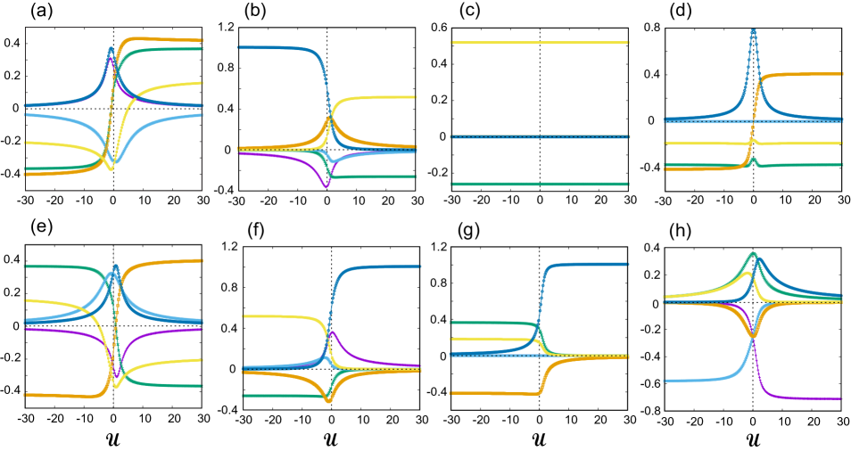
Figure 12: The six different ${\cal C}$-coefficients (dimensionless) [see Eq. (44)] for the eight remaining excited eigenstates of 3 bosons trapped in 3 linearly arranged wells as a function of ${\cal U}$ (horizontal axis, dimensionless). This figure complements Fig. 3 in the main text. (a) $i=3r(4l)$. (b) $i=4r(3l)$. (c) $i=5r(6l)$. (d) $i=6r(5l)$. (e) $i=7r(8l)$. (f) $i=8r(7l)$. (g) $i=9$. (h) $i=10$. The choice of online colors is the same as in Fig. 3, that is: ${\cal C}_{0}\rightarrow$ Violet, ${\cal C}_{1}\rightarrow$ Green, ${\cal C}_{1-1}\rightarrow$ Light Blue, ${\cal C}_{1+1}\rightarrow$ Brown, ${\cal C}_{1+1-1}\rightarrow$ Yellow, ${\cal C}_{1+1+1}\rightarrow$ Dark Blue. For the print grayscale version, the positioning (referred to as #$n$, with $n=1,2,3,\dots$) of the curves from top to bottom at the point ${\cal U}=-30$ is as follows: (a) ${\cal C}_{0}\rightarrow$ #2 (overlaps with #1), ${\cal C}_{1}\rightarrow$ #5, ${\cal C}_{1-1}\rightarrow$ #3, ${\cal C}_{1+1}\rightarrow$ #6, ${\cal C}_{1+1-1}\rightarrow$ #4, ${\cal C}_{1+1+1}\rightarrow$ #1 (overlaps with #2). (b) ${\cal C}_{0}\rightarrow$ #6, ${\cal C}_{1}\rightarrow$ #5 (overlaps with #3 and #4), ${\cal C}_{1-1}\rightarrow$ #4, ${\cal C}_{1+1}\rightarrow$ #2, ${\cal C}_{1+1-1}\rightarrow$ #3, ${\cal C}_{1+1+1}\rightarrow$ #1. (c) ${\cal C}_{0}={\cal C}_{1-1}={\cal C}_{1+1}={\cal C}_{1+1+1}=0$, ${\cal C}_{1}\rightarrow$ lower curve, ${\cal C}_{1+1-1}\rightarrow$ upper curve. (d) ${\cal C}_{0}\rightarrow$ #3 (overlaps with #2), ${\cal C}_{1}\rightarrow$ #5, ${\cal C}_{1-1}\rightarrow$ #2, ${\cal C}_{1+1}\rightarrow$ #6, ${\cal C}_{1+1-1}\rightarrow$ #4, ${\cal C}_{1+1+1}\rightarrow$ #1. (e) ${\cal C}_{0}\rightarrow$ #5, ${\cal C}_{1}\rightarrow$ #1, ${\cal C}_{1-1}\rightarrow$ #3, ${\cal C}_{1+1}\rightarrow$ #6, ${\cal C}_{1+1-1}\rightarrow$ #2, ${\cal C}_{1+1+1}\rightarrow$ #4. (f) ${\cal C}_{0}\rightarrow$ #3 (overlaps with #2), ${\cal C}_{1}\rightarrow$ #6, ${\cal C}_{1-1}\rightarrow$ #2, ${\cal C}_{1+1}\rightarrow$ #5, ${\cal C}_{1+1-1}\rightarrow$ #1, ${\cal C}_{1+1+1}\rightarrow$ #4. (g) ${\cal C}_{0}\rightarrow$ #5 (overlaps with #4), ${\cal C}_{1}\rightarrow$ #1, ${\cal C}_{1-1}\rightarrow$ #4, ${\cal C}_{1+1}\rightarrow$ #6, ${\cal C}_{1+1-1}\rightarrow$ #2, ${\cal C}_{1+1+1}\rightarrow$ #3. (h) ${\cal C}_{0}\rightarrow$ #4 (overlaps with #3 and #5), ${\cal C}_{1}\rightarrow$ #1 (overlaps with #2), ${\cal C}_{1-1}\rightarrow$ #6, ${\cal C}_{1+1}\rightarrow$ #5, ${\cal C}_{1+1-1}\rightarrow$ #2, ${\cal C}_{1+1+1}\rightarrow$ #3.

Appendix E Third-order momentum correlations as a function of ${\cal U}$ for the remaining eight excited states

Fig. 12 complements Fig. 3 in that it displays the six coefficients ${\cal C}^{i}({\cal U})$’s for the remaining eight excited states (explicit numerical values can be found in the supplemental material supp ). The dependence of these coefficients on the interaction strength ${\cal U}$ is better deciphered by using as reference points the special cases at ${\cal U}\rightarrow\pm\infty$ and ${\cal U}=0$. Note that in all cases the ${\cal C}^{i}$ values at the end points ${\cal U}=\pm 30$ in the figure are close to the corresponding limiting values at ${\cal U}\rightarrow\pm\infty$. In particular,

The excited state denoted as $i=3r(4l)$ ($i=3$ for $0<{\cal U}<+\infty$ and $i=4$ for $-\infty<{\cal U}<0$): For ${\cal U}\rightarrow-\infty$, only three coefficients, ${{\cal C}}^{4,-\infty}_{1}=-2\times 2^{3/4}/(\sqrt{15}\pi^{3/4})=-0.3680$, ${{\cal C}}^{4,-\infty}_{1+1}=-2^{3/4}/(\sqrt{3}\pi^{3/4})=-0.4115$, and ${{\cal C}}^{4,-\infty}_{1+1-1}=-2^{3/4}/(\sqrt{15}\pi^{3/4})=-0.1840$, survive in expression (44) [see frame (a) in Fig. 12]; the corresponding Hubbard eigenvector, $\phi^{b,-\infty}_{4}$ [second line in Eq. (68)] consists of all 6 primitive kets [see Eq. (1)] representing exclusively doubly-occupied wells, and the corresponding wave function in momentum space has 9 cosinusoidal terms and is given by the second expression in Eq. (84).

For ${\cal U}=0$, all 6 coefficients, ${\cal C}^{3r(4l),{\cal U}=0}$’s, are present, and their numerical values from frame (a) in Fig. 12 agree with the numerical values for $\Phi_{3r(4l)}^{b,{\cal U}=0}(k_{1},k_{2},k_{3})$ in Eq. (91).

For ${\cal U}\rightarrow+\infty$, again only three coefficients, ${{\cal C}}^{3,+\infty}_{1}=2\times 2^{3/4}/(\sqrt{15}\pi^{3/4})=0.3680$, ${{\cal C}}^{3,+\infty}_{1+1}=2^{3/4}/(\sqrt{3}\pi^{3/4})=0.4115$, and ${{\cal C}}^{3,+\infty}_{1+1-1}=2^{3/4}/(\sqrt{15}\pi^{3/4})=0.1840$, survive in expression (44) [see frame (a) in Fig. 12]; the corresponding Hubbard eigenvector, $\phi^{b,+\infty}_{3}$ [first line in Eq. (67)] consists of all 6 primitive kets [see Eq. (1)] representing exclusively doubly-occupied wells, and the corresponding wave function in momentum space has 9 cosinusoidal terms and is given by the second expression in Eq. (83).

The excited state denoted as $i=4r(3l)$ ($i=4$ for $0<{\cal U}<+\infty$ and $i=3$ for $-\infty<{\cal U}<0$): For ${\cal U}\rightarrow-\infty$, only one coefficient, ${{\cal C}}^{3,-\infty}_{1+1+1}=2\times 2^{1/4}/\pi^{3/4}=1.0079$, survives in expression (44) (see frame (b) in Fig. 12); the corresponding Hubbard eigenvector, $\phi^{b,-\infty}_{3}$ [second line in Eq. (67)] is a NOON state of the form $(|300\rangle+|003\rangle)/\sqrt{2}$, and the corresponding wave function in momentum space is given by the second expression in Eq. (83), which includes a cos term only.

For ${\cal U}=0$, all 6 coefficients, ${\cal C}^{4r(3l),{\cal U}=0}$’s, are present, and their numerical values from frame (b) in Fig. 12 agree with the numerical values for $\Phi_{4r(3l)}^{b,{\cal U}=0}(k_{1},k_{2},k_{3})$ in Eq. (92).

For ${\cal U}\rightarrow+\infty$, only two coefficients, ${{\cal C}}^{4,+\infty}_{1}=-2\times 2^{1/4}/(\sqrt{15}\pi^{3/4})=-0.2602$, and ${{\cal C}}^{4,+\infty}_{1+1-1}=4\times 2^{1/4}/(\sqrt{15}\pi^{3/4})=0.5205$, survive in expression (44) [see frame (b) in Fig. 12]; the corresponding Hubbard eigenvector, $\phi^{b,+\infty}_{4}$ [first line in Eq. (68)] consists of 4 primitive kets [see Eq. (1)] representing exclusively doubly-occupied wells, and the corresponding wave function in momentum space has 6 cosinusoidal terms and is given by the first expression in Eq. (84).

The excited state denoted as $i=5r(6l)$ ($i=5$ for $0<{\cal U}<+\infty$ and $i=6$ for $-\infty<{\cal U}<0$): The Hubbard eigenvector solution for this state state is ${\cal U}$-independent; see first expression in Eq. (69), second expression in Eq. (70), or Eq. (77). In this case, 2 distinct coefficients survive in expression (44), that is, ${{\cal C}}^{6,-\infty}_{1}={{\cal C}}^{5,+\infty}_{1}={{\cal C}}^{5r(6l),{\cal U}=0}_{1}=-2\times 2^{1/4}/(\sqrt{15}\pi^{3/4})=-0.2602$, and ${{\cal C}}^{6,-\infty}_{1+1-1}={{\cal C}}^{5,+\infty}_{1+1-1}={{\cal C}}^{5r(6l),{\cal U}=0}_{1+1-1}=4\times 2^{1/4}/(\sqrt{15}\pi^{3/4})=0.5205$, in agreement with frame (c) in Fig. 12. The corresponding Hubbard eigenvectors, $\phi^{b,+\infty}_{5}=\phi^{b,-\infty}_{6}=\phi^{b,{\cal U}=0}_{5r(6l)}$, consist of 4 primitive kets [see Eq. (1)] representing exclusively doubly-occupied wells, and the corresponding wave function in momentum space has 6 cosinusoidal terms and is given by the second expression in Eq. (86) or the first expression in Eq. (85).

The excited state denoted as $i=6r(5l)$ ($i=6$ for $0<{\cal U}<+\infty$ and $i=5$ for $-\infty<{\cal U}<0$): For ${\cal U}\rightarrow-\infty$, only three coefficients, ${{\cal C}}^{5,-\infty}_{1}=-2\times 2^{3/4}/(\sqrt{15}\pi^{3/4})=-0.3680$, ${{\cal C}}^{5,-\infty}_{1+1}=-2^{3/4}/(\sqrt{3}\pi^{3/4})=-0.4115$, and ${{\cal C}}^{5,-\infty}_{1+1-1}=-2^{3/4}/(\sqrt{15}\pi^{3/4})=-0.1840$, survive in expression (44) [see frame (d) in Fig. 12]; the corresponding Hubbard eigenvector, $\phi^{b,-\infty}_{5}$ [second line in Eq. (69)] consists of all 6 primitive kets [see Eq. (1)] representing exclusively doubly-occupied wells, and the corresponding wave function in momentum space has 9 sinusoidal terms and is given by the second expression in Eq. (85).

For ${\cal U}=0$, three coefficients are present, namely ${{\cal C}}^{6r(5l),{\cal U}=0}_{1}$, ${{\cal C}}^{6r(5l),{\cal U}=0}_{1+1-1}$, and ${{\cal C}}^{6r(5l),{\cal U}=0}_{1+1+1}$. Their numerical values from frame (d) in Fig. 12 agree with the corresponding algebraic expressions for $\Phi_{6r(5l)}^{b,{\cal U}=0}(k_{1},k_{2},k_{3})$ in Eq. (94).

For ${\cal U}\rightarrow+\infty$, again only three coefficients, ${{\cal C}}^{6,+\infty}_{1}=-2\times 2^{3/4}/(\sqrt{15}\pi^{3/4})=-0.3680$, ${{\cal C}}^{6,+\infty}_{1+1}=2^{3/4}/(\sqrt{3}\pi^{3/4})=0.4115$, and ${{\cal C}}^{6,+\infty}_{1+1-1}=-2^{3/4}/(\sqrt{15}\pi^{3/4})=-0.1840$, survive in expression (44) [see frame (d) in Fig. 12]; the corresponding Hubbard eigenvector, $\phi^{b,+\infty}_{6}$ [first line in Eq. (70)] consists of all 6 primitive kets [see Eq. (1)] representing exclusively doubly-occupied wells, and the corresponding wave function in momentum space has 9 sinusoidal terms and is given by the first expression in Eq. (86).

The excited state denoted as $i=7r(8l)$ ($i=7$ for $0<{\cal U}<+\infty$ and $i=8$ for $-\infty<{\cal U}<0$): For ${\cal U}\rightarrow-\infty$, only three coefficients, ${{\cal C}}^{8,-\infty}_{1}=2\times 2^{3/4}/(\sqrt{15}\pi^{3/4})=0.3680$, ${{\cal C}}^{8,-\infty}_{1+1}=-2^{3/4}/(\sqrt{3}\pi^{3/4})=-0.4115$, and ${{\cal C}}^{8,-\infty}_{1+1-1}=2^{3/4}/(\sqrt{15}\pi^{3/4})=0.1840$, survive in expression (44) [see sixth frame (e) in Fig. 12]; the corresponding Hubbard eigenvector, $\phi^{b,-\infty}_{8}$ [second line in Eq. (72)] consists of all 6 primitive kets [see Eq. (1)] representing exclusively doubly-occupied wells, and the corresponding wave function in momentum space has 9 cosinusoidal terms and is given by the second expression in Eq. (88).

For ${\cal U}=0$, all 6 coefficients, ${\cal C}^{7r(8l),{\cal U}=0}$’s, are present, and their numerical values from frame (e) in Fig. 12 agree with the numerical values for $\Phi_{7r(8l)}^{b,{\cal U}=0}(k_{1},k_{2},k_{3})$ in Eq. (95).

For ${\cal U}\rightarrow+\infty$, again only three coefficients, ${{\cal C}}^{7,+\infty}_{1}=-2\times 2^{3/4}/(\sqrt{15}\pi^{3/4})=-0.3680$, ${{\cal C}}^{7,+\infty}_{1+1}=2^{3/4}/(\sqrt{3}\pi^{3/4})=0.4115$, and ${{\cal C}}^{7,+\infty}_{1+1-1}=-2^{3/4}/(\sqrt{15}\pi^{3/4})=-0.1840$, survive in expression (44) [see frame (e) in Fig. 12]; the corresponding Hubbard eigenvector, $\phi^{b,+\infty}_{7}$ [first line in Eq. (71)] consists of all 6 primitive kets [see Eq. (1)] representing exclusively doubly-occupied wells, and the corresponding wave function in momentum space has 9 cosinusoidal terms and is given by the first expression in Eq. (87).

The excited state denoted as $i=8r(7l)$ ($i=8$ for $0<{\cal U}<+\infty$ and $i=7$ for $-\infty<{\cal U}<0$): For ${\cal U}\rightarrow-\infty$, only two coefficients, ${{\cal C}}^{7,-\infty}_{1}=-2\times 2^{1/4}/(\sqrt{15}\pi^{3/4})=-0.2602$, and ${{\cal C}}^{7,-\infty}_{1+1-1}=4\times 2^{1/4}/(\sqrt{15}\pi^{3/4})=0.5205$, survive in expression (44) [see frame (f) in Fig. 12]; the corresponding Hubbard eigenvector, $\phi^{b,-\infty}_{7}$ [second line in Eq. (71)] consists of 4 primitive kets [see Eq. (1)] representing exclusively doubly-occupied wells, and the corresponding wave function in momentum space has 6 cosinusoidal terms and is given by the second expression in Eq. (87).

For ${\cal U}=0$, all 6 coefficients, ${\cal C}^{8r(7l),{\cal U}=0}$’s, are present, and their numerical values from frame (f) in Fig. 12 agree with the numerical values for $\Phi_{8r(7l)}^{b,{\cal U}=0}(k_{1},k_{2},k_{3})$ in Eq. (96).

For ${\cal U}\rightarrow+\infty$, only one coefficient, ${{\cal C}}^{8,+\infty}_{1+1+1}=2\times 2^{1/4}/\pi^{3/4}=1.0079$, survives in expression (44) [see frame (f) in Fig. 12]; the corresponding Hubbard eigenvector, $\phi^{b,+\infty}_{8}$ [first line in Eq. (72)] is a NOON state of the form $(|300\rangle+|003\rangle)/\sqrt{2}$, and the corresponding wave function in momentum space is given by the first expression in Eq. (88), which includes a cos term only.

The excited state denoted as $i=9$ for $-\infty<{\cal U}<+\infty$: For ${\cal U}\rightarrow-\infty$, only three coefficients, ${{\cal C}}^{5,-\infty}_{1}=2\times 2^{3/4}/(\sqrt{15}\pi^{3/4})=0.3680$, ${{\cal C}}^{5,-\infty}_{1+1}=-2^{3/4}/(\sqrt{3}\pi^{3/4})=-0.4115$, and ${{\cal C}}^{5,-\infty}_{1+1-1}=2^{3/4}/(\sqrt{15}\pi^{3/4})=0.1840$, survive in expression (44) [see frame (g) in Fig. 12]; the corresponding Hubbard eigenvector, $\phi^{b,-\infty}_{9}$ [second line in Eq. (73)] consists of all 6 primitive kets [see Eq. (1)] representing exclusively doubly-occupied wells, and the corresponding wave function in momentum space has 9 sinusoidal terms and is given by the second expression in Eq. (89).

For ${\cal U}=0$, four coefficients are present, namely ${{\cal C}}^{9,{\cal U}=0}_{1}$, ${{\cal C}}^{9,{\cal U}=0}_{1+1}$, ${{\cal C}}^{9,{\cal U}=0}_{1+1-1}$, and ${{\cal C}}^{9,{\cal U}=0}_{1+1+1}$. Their numerical values from frame (g) in Fig. 12 agree with the corresponding algebraic expressions for $\Phi_{9}^{b,{\cal U}=0}(k_{1},k_{2},k_{3})$ in Eq. (97).

For ${\cal U}\rightarrow+\infty$, only one coefficient, ${{\cal C}}^{9,+\infty}_{1+1+1}=2\times 2^{1/4}/\pi^{3/4}=1.0079$, survives in expression (44) [see frame (g) in Fig. 12]; the corresponding Hubbard eigenvector, $\phi^{b,+\infty}_{9}$ [first line in Eq. (73)] is a NOON state of the form $(-|300\rangle+|003\rangle)/\sqrt{2}$, and the corresponding wave function in momentum space is given by the first expression in Eq. (89), which includes a sin term only.

The highest excited state denoted as $i=10$ for $-\infty<{\cal U}<+\infty$: For ${\cal U}\rightarrow-\infty$, only the coefficient ${\cal C}^{10,-\infty}_{1-1}=-2\times 2^{1/4}/(\sqrt{3}\pi^{3/4})=-0.5819$ survives in expression (44); see frame (h) in Fig. 12. The corresponding momentum-space wave function comprises three cosinusoidal terms and is given by the second expression in Eq. (90). The corresponding Hubbard eigenvector $\phi^{b,-\infty}_{10}$ [second line in Eq. (74)] contains only a single component from the primitive kets listed in Eq. (1), i.e., the basis ket No. 1 $\rightarrow|111\rangle$, reflecting the fact that all three wells are singly occupied.

For ${\cal U}=0$, all 6 coefficients, ${\cal C}^{10,{\cal U}=0}$’s, are present, and their numerical values from frame (h) in Fig. 12 agree with the numerical values for $\Phi_{10}^{b,{\cal U}=0}(k_{1},k_{2},k_{3})$ in Eq. (98).

For ${\cal U}\rightarrow+\infty$, it is seen from frame (h) in Fig. 12 that only the constant coefficient ${\cal C}^{10,-\infty}_{0}=-(2/\pi)^{3/4}=-0.7127$ survives in expression (44); the corresponding wave function in momentum space is given by the first expression in Eq. (90). It is a simple Gaussian distribution associated with a Bose-Einstein condensate, reflecting the fact that all three bosons are localized in the middle well and occupy the same orbital; the corresponding Hubbard eigenvector is given by $\phi^{b,+\infty}_{10}$ [first line in Eq. (74)] which contains only a single component from the primitive kets listed in Eq. (1), i.e., the basis ket No. 9 $\rightarrow|030\rangle$.

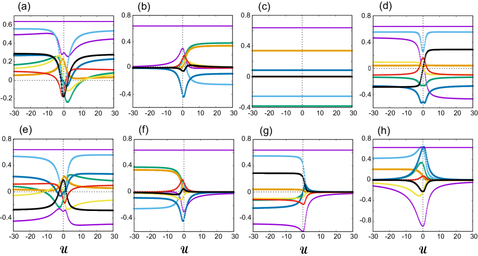
Figure 13: The nine ${\cal B}$-coefficients (dimensionless) [see Eq. (46)] for the remaining 8 excited eigenstates of 3 bosons trapped in 3 linearly arranged wells as a function of ${\cal U}$ (horizontal axis, dimensionless). This figure complements Fig. 5 in the main text. (a) $i=3r(4l)$. (b) $i=4r(3l)$. (c) $i=5r(6l)$. (d) $i=6r(5l)$. (e) $i=7r(8l)$. (f) $i=8r(7l)$, (g) $i=9$, (h) $i=10$. See text for a detailed description. The choice of colors is the same as in Fig. 5, that is: ${\cal B}_{0}\rightarrow$ Constant (Violet), ${\cal B}_{1}\rightarrow$ Second Violet, ${\cal B}_{2}\rightarrow$ Green, ${\cal B}_{1-1}\rightarrow$ Light Blue, ${\cal B}_{2-2}\rightarrow$ Brown, ${\cal B}_{2-1}\rightarrow$ Yellow, ${\cal B}_{1+1}\rightarrow$ Dark Blue, ${\cal B}_{2+2}\rightarrow$ Red, ${\cal B}_{2+1}\rightarrow$ Black. For the print grayscale version, the positioning (referred to as #$n$, with $n=1,2,3,\dots$) of the curves from top to bottom at the point ${\cal U}=-30$ is as follows: (a) ${\cal B}_{0}\rightarrow$ #1, ${\cal B}_{1}\rightarrow$ #3, ${\cal B}_{2}\rightarrow$ #6, ${\cal B}_{1-1}\rightarrow$ #2, ${\cal B}_{2-2}\rightarrow$ #9, ${\cal B}_{2-1}\rightarrow$ #7, ${\cal B}_{1+1}\rightarrow$ #5, ${\cal B}_{2+2}\rightarrow$ #8, ${\cal B}_{2+1}\rightarrow$ #4. (b) ${\cal B}_{0}\rightarrow$ #1, ${\cal B}_{1}\rightarrow$ #2, ${\cal B}_{2}\rightarrow$ #5 (overlaps with #3, #4, #6, #7, #8, #9), ${\cal B}_{1-1}\rightarrow$ #4, ${\cal B}_{2-2}\rightarrow$ #7, ${\cal B}_{2-1}\rightarrow$ #6, ${\cal B}_{1+1}\rightarrow$ #9, ${\cal B}_{2+2}\rightarrow$ #3, ${\cal B}_{2+1}\rightarrow$ #8. (c) ${\cal B}_{0}\rightarrow$ #1, ${\cal B}_{1}\rightarrow$ #4 (overlaps with #5, #6, #7), ${\cal B}_{2}\rightarrow$ #9, ${\cal B}_{1-1}\rightarrow$ #8, ${\cal B}_{2-2}\rightarrow$ #2, ${\cal B}_{2-1}\rightarrow$ #5, ${\cal B}_{1+1}\rightarrow$ #3, ${\cal B}_{2+2}\rightarrow$ #6, ${\cal B}_{2+1}\rightarrow$ #7. (d) ${\cal B}_{0}\rightarrow$ #1, ${\cal B}_{1}\rightarrow$ #3, ${\cal B}_{2}\rightarrow$ #7, ${\cal B}_{1-1}\rightarrow$ #2, ${\cal B}_{2-2}\rightarrow$ #5, ${\cal B}_{2-1}\rightarrow$ #4, ${\cal B}_{1+1}\rightarrow$ #8, ${\cal B}_{2+2}\rightarrow$ #6, ${\cal B}_{2+1}\rightarrow$ #9. (e) ${\cal B}_{0}\rightarrow$ #1, ${\cal B}_{1}\rightarrow$ #9, ${\cal B}_{2}\rightarrow$ #5, ${\cal B}_{1-1}\rightarrow$ #2, ${\cal B}_{2-2}\rightarrow$ #6, ${\cal B}_{2-1}\rightarrow$ #7, ${\cal B}_{1+1}\rightarrow$ #3, ${\cal B}_{2+2}\rightarrow$ #4, ${\cal B}_{2+1}\rightarrow$ #8. (f) ${\cal B}_{0}\rightarrow$ #1, ${\cal B}_{1}\rightarrow$ #5 (overlaps with #4, #6, #7), ${\cal B}_{2}\rightarrow$ #2, ${\cal B}_{1-1}\rightarrow$ #9, ${\cal B}_{2-2}\rightarrow$ #3, ${\cal B}_{2-1}\rightarrow$ #7, ${\cal B}_{1+1}\rightarrow$ #8, ${\cal B}_{2+2}\rightarrow$ #4, ${\cal B}_{2+1}\rightarrow$ #6. (g) ${\cal B}_{0}\rightarrow$ #1, ${\cal B}_{1}\rightarrow$ #9, ${\cal B}_{2}\rightarrow$ #7 (overlaps with #5, #6), ${\cal B}_{1-1}\rightarrow$ #2, ${\cal B}_{2-2}\rightarrow$ #4, ${\cal B}_{2-1}\rightarrow$ #5, ${\cal B}_{1+1}\rightarrow$ #8, ${\cal B}_{2+2}\rightarrow$ #6, ${\cal B}_{2+1}\rightarrow$ #3. (h) ${\cal B}_{0}\rightarrow$ #1, ${\cal B}_{1}\rightarrow$ #9, ${\cal B}_{2}\rightarrow$ #5 (overlaps wih #4), ${\cal B}_{1-1}\rightarrow$ #2, ${\cal B}_{2-2}\rightarrow$ #3, ${\cal B}_{2-1}\rightarrow$ #8, ${\cal B}_{1+1}\rightarrow$ #4, ${\cal B}_{2+2}\rightarrow$ #6 (overlaps with #7), ${\cal B}_{2+1}\rightarrow$ #7.

Appendix F Second-order momentum correlations as a function of ${\cal U}$ for the remaining eight excited states

Fig. 13 complements Fig. 5 in that it displays the 9 distinct coefficients ${\cal B}^{i}({\cal U})$’s for the remaining eight excited states (explicit numerical values can be found in the supplemental material supp ). The dependence of these coefficients on the interaction strength ${\cal U}$ is better deciphered by using as reference points the special cases at ${\cal U}\rightarrow\pm\infty$ and ${\cal U}=0$. Note that in all cases the ${\cal B}^{i}$ values at the end points ${\cal U}=\pm 30$ in the figure are close to the corresponding limiting values at ${\cal U}\rightarrow\pm\infty$. In particular,

The excited state denoted as $i=3r(4l)$ ($i=3$ for $0<{\cal U}<+\infty$ and $i=4$ for $-\infty<{\cal U}<0$)): For ${\cal U}\rightarrow-\infty$ all 9 distinct coefficients survive [see frame (a) in Fig. 13]; this state consists of only doubly-and-singly occupied sites [see second line of Eq. (68)]. In this case, the 9 distinct coefficients are: ${\cal B}^{4,-\infty}_{0}=2/\pi$, ${\cal B}^{4,-\infty}_{1}=2\sqrt{5}/(3\pi)$, ${\cal B}^{4,-\infty}_{2}=2/(5\pi)$, ${\cal B}^{4,-\infty}_{1-1}=26/(15\pi)$, ${\cal B}^{4,-\infty}_{2-2}=2/(15\pi)$, ${\cal B}^{4,-\infty}_{2-1}=2/(3\sqrt{5}\pi)$, ${\cal B}^{4,-\infty}_{1+1}=4/(5\pi)$, ${\cal B}^{4,-\infty}_{2+2}=1/(3\pi)$, and ${\cal B}^{4,-\infty}_{2+1}=2/(\sqrt{5}\pi)$.

In the noninteracting case (${\cal U}=0$), for which the Hubbard eigenvector is given by Eq. (75), all 13 cosinusoidal terms and 9 distinct coefficients are present in Eq. (46), in agreement with the frame (a) of Fig. 13, that is, ${\cal B}^{3r(4l),{\cal U}=0}_{0}=2/\pi=0.63662$, ${\cal B}^{3r(4l),{\cal U}=0}_{1}=0.300105$, ${\cal B}^{3r(4l),{\cal U}=0}_{2}=-0.111766$, ${\cal B}^{3r(4l),{\cal U}=0}_{1-1}=-0.124185$, ${\cal B}^{3r(4l),{\cal U}=0}_{2-2}=0.214057$, ${\cal B}^{3r(4l),{\cal U}=0}_{2-1}=0.0243414$, ${\cal B}^{3r(4l),{\cal U}=0}_{1+1}=-0.0135114$, ${\cal B}^{3r(4l),{\cal U}=0}_{2+2}=-0.127997$, and ${\cal B}^{3r(4l),{\cal U}=0}_{2+1}=-0.178398$.

For ${\cal U}\rightarrow+\infty$, all 13 cosinusoidal terms survive in expression (46); the corresponding state is given by the first expression in Eq. (67). In this case, the 9 distinct coefficients are: ${\cal B}^{3,+\infty}_{0}=2/\pi$, ${\cal B}^{3,+\infty}_{1}=2\sqrt{5}/(3\pi)$, ${\cal B}^{3,+\infty}_{2}=2/(5\pi)$, ${\cal B}^{3,+\infty}_{1-1}=26/(15\pi)$, ${\cal B}^{3,+\infty}_{2-2}=2/(15\pi)$, ${\cal B}^{3,+\infty}_{2-1}=2/(3\sqrt{5}\pi)$, ${\cal B}^{3,+\infty}_{1+1}=4/(5\pi)$, ${\cal B}^{3,+\infty}_{2+2}=1/(3\pi)$, and ${\cal B}^{3,+\infty}_{2+1}=2/(\sqrt{5}\pi)$.

We note that ${}^{2}{\cal G}_{4}^{b,-\infty}(k_{1},k_{2})\;=\;^{2}{\cal G}_{3}^{b,+\infty}(k_{1},k_{2})$.

The excited state denoted as $i=4r(3l)$ ($i=4$ for $0<{\cal U}<+\infty$ and $i=3$ for $-\infty<{\cal U}<0$): For ${\cal U}\rightarrow-\infty$ only the constant term survives in expression (46); the corresponding state is given by the second expression in Eq. (67) and is a NOON state of the form $(|300\rangle+|003\rangle)/\sqrt{2}$. In this case, the second-order correlation function is given by:

$${}^{2}{\cal G}_{3}^{b,-\infty}(k_{1},k_{2})=\frac{2}{\pi}s^{2}e^{-2(k_{1}^{2}+k_{2}^{2})s^{2}}.$$ (99)

In the noninteracting case (${\cal U}=0$), for which the Hubbard eigenvector is given by Eq. (76), all 13 cosinusoidal terms and 9 distinct coefficients are present in Eq. (46), in agreement with the frame (b) of Fig. 13, that is, ${\cal B}^{4r(3l),{\cal U}=0}_{0}=2/\pi=0.63662$, ${\cal B}^{4r(3l),{\cal U}=0}_{1}=0.300105$, ${\cal B}^{4r(3l),{\cal U}=0}_{2}=0.111766$, ${\cal B}^{4r(3l),{\cal U}=0}_{1-1}=0.124185$, ${\cal B}^{4r(3l),{\cal U}=0}_{2-2}=0.0246755$, ${\cal B}^{4r(3l),{\cal U}=0}_{2-1}=0.0506849$, ${\cal B}^{4r(3l),{\cal U}=0}_{1+1}=-0.410902$, ${\cal B}^{4r(3l),{\cal U}=0}_{2+2}=0.154523$, and ${\cal B}^{4r(3l),{\cal U}=0}_{2+1}=-0.0466808$.

For ${\cal U}\rightarrow+\infty$, 6 cosinusoidal terms survive in expression (46); see frame (b) in Fig. 13. The corresponding state is given by the first expression in Eq. (68). In this case, the 5 non-zero distinct coefficients are: ${\cal B}^{4,+\infty}_{0}=2/\pi$, ${\cal B}^{4,+\infty}_{1}=0$, ${\cal B}^{4,+\infty}_{2}=6/(5\pi)$, ${\cal B}^{4,+\infty}_{1-1}=-4/(5\pi)$, ${\cal B}^{4,+\infty}_{2-2}=16/(15\pi)$, ${\cal B}^{4,+\infty}_{2-1}=0$, ${\cal B}^{4,+\infty}_{1+1}=-4/(15\pi)$, ${\cal B}^{4,+\infty}_{2+2}=0$, and ${\cal B}^{4,+\infty}_{2+1}=0$.

The excited state denoted as $i=5r(6l)$ ($i=5$ for $0<{\cal U}<+\infty$ and $i=6$ for $-\infty<{\cal U}<0$): This state is ${\cal U}$-independent; see first expression in Eq. (69) or second expression in Eq. (70). In this case, 5 distinct coefficients (corresponding to 6 cosinusoidal terms) survive in expression (46), that is, ${\cal B}^{5,+\infty}_{0}={\cal B}^{6,-\infty}_{0}={\cal B}^{5r(6l),{\cal U}=0}_{0}=2/\pi$, ${\cal B}^{5,+\infty}_{1}={\cal B}^{6,-\infty}_{1}={\cal B}^{5r(6l),{\cal U}=0}_{1}=0$, ${\cal B}^{5,+\infty}_{2}={\cal B}^{6,-\infty}_{2}={\cal B}^{5r(6l),{\cal U}=0}_{2}=-6/(5\pi)$, ${\cal B}^{5,+\infty}_{1-1}={\cal B}^{6,-\infty}_{1-1}={\cal B}^{5r(6l),{\cal U}=0}_{1-1}=-4/(5\pi)$, ${\cal B}^{5,+\infty}_{2-2}={\cal B}^{6,-\infty}_{2-2}={\cal B}^{5r(6l),{\cal U}=0}_{2-2}=16/(15\pi)$, ${\cal B}^{5,+\infty}_{2-1}={\cal B}^{6,-\infty}_{2-1}={\cal B}^{5r(6l),{\cal U}=0}_{2-1}=0$, ${\cal B}^{5,+\infty}_{1+1}={\cal B}^{6,-\infty}_{1+1}={\cal B}^{5r(6l),{\cal U}=0}_{1+1}=4/(15\pi)$, ${\cal B}^{5,+\infty}_{2+2}={\cal B}^{6,-\infty}_{2+2}={\cal B}^{5r(6l),{\cal U}=0}_{2+2}=0$, and ${\cal B}^{5,+\infty}_{2+1}={\cal B}^{6,-\infty}_{2+1}={\cal B}^{5r(6l),{\cal U}=0}_{2+1}=0$; see frame (c) in Fig. 13.

The excited state denoted as $i=6r(5l)$ ($i=6$ for $0<{\cal U}<+\infty$ and $i=5$ for $-\infty<{\cal U}<0$): For ${\cal U}\rightarrow-\infty$, all 9 distinct coefficients [see frame (d) in Fig. 13] and 13 cosinusoidal terms survive in expression (46); the corresponding state is given by the second expression in Eq. (69). In this case, the 9 distinct coefficients are: ${\cal B}^{5,-\infty}_{0}=2/\pi$, ${\cal B}^{5,-\infty}_{1}=2\sqrt{5}/(3\pi)$, ${\cal B}^{5,-\infty}_{2}=-2/(5\pi)$, ${\cal B}^{5,-\infty}_{1-1}=26/(15\pi)$, ${\cal B}^{5,-\infty}_{2-2}=2/(15\pi)$, ${\cal B}^{5,-\infty}_{2-1}=2/(3\sqrt{5}\pi)$, ${\cal B}^{5,-\infty}_{1+1}=-4/(5\pi)$, ${\cal B}^{5,-\infty}_{2+2}=-1/(3\pi)$, and ${\cal B}^{5,-\infty}_{2+1}=-2/(\sqrt{5}\pi)$.

In the noninteracting case (${\cal U}=0$), for which the Hubbard eigenvector is given by Eq. (78), 6 distinct coefficients (corresponding to 7 cosinusoidal terms) are present in expression (46), in agreement with frame (d) of Fig. 13. That is, ${\cal B}^{6r(5l),{\cal U}=0}_{0}=2/\pi=0.63662$, ${\cal B}^{6r(5l),{\cal U}=0}_{1}=0$, ${\cal B}^{6r(5l),{\cal U}=0}_{2}=-4/(5\pi)$, ${\cal B}^{6r(5l),{\cal U}=0}_{1-1}=4/(5\pi)$, ${\cal B}^{6r(5l),{\cal U}=0}_{2-2}=1/(10\pi)$, ${\cal B}^{6r(5l),{\cal U}=0}_{2-1}=0$, ${\cal B}^{6r(5l),{\cal U}=0}_{1+1}=-8/(5\pi)$, ${\cal B}^{6r(5l),{\cal U}=0}_{2+2}=1/(2\pi)$, and ${\cal B}^{6r(5l),{\cal U}=0}_{2+1}=0$.

For ${\cal U}\rightarrow+\infty$, all 13 cosinusoidal terms survive in expression (46); the corresponding state is given by the first expression in Eq. (70). In this case, in agreement with the frame (d) of Fig. 13, the 9 distinct coefficients are: ${\cal B}^{6,+\infty}_{0}=2/\pi$, ${\cal B}^{6,+\infty}_{1}=-2\sqrt{5}/(3\pi)$, ${\cal B}^{6,+\infty}_{2}=-2/(5\pi)$, ${\cal B}^{6,+\infty}_{1-1}=26/(15\pi)$, ${\cal B}^{6,+\infty}_{2-2}=2/(15\pi)$, ${\cal B}^{6,+\infty}_{2-1}=-2/(3\sqrt{5}\pi)$, ${\cal B}^{6,+\infty}_{1+1}=-4/(5\pi)$, ${\cal B}^{6,+\infty}_{2+2}=-1/(3\pi)$, and ${\cal B}^{6,+\infty}_{2+1}=2/(\sqrt{5}\pi)$.

The excited state denoted as $i=7r(8l)$ ($i=7$ for $0<{\cal U}<+\infty$ and $i=8$ for $-\infty<{\cal U}<0$): For ${\cal U}\rightarrow-\infty$, all 9 distinct coefficients [see frame (e) in Fig. 13] and 13 cosinusoidal terms survive in expression (46); the corresponding state is given by the second expression in Eq. (72). In this case, the 9 distinct coefficients are: ${\cal B}^{8,-\infty}_{0}=2/\pi$, ${\cal B}^{8,-\infty}_{1}=-2\sqrt{5}/(3\pi)$, ${\cal B}^{8,-\infty}_{2}=2/(5\pi)$, ${\cal B}^{8,-\infty}_{1-1}=26/(15\pi)$, ${\cal B}^{8,-\infty}_{2-2}=2/(15\pi)$, ${\cal B}^{8,-\infty}_{2-1}=-2/(3\sqrt{5}\pi)$, ${\cal B}^{8,-\infty}_{1+1}=4/(5\pi)$, ${\cal B}^{8,-\infty}_{2+2}=1/(3\pi)$, and ${\cal B}^{8,-\infty}_{2+1}=-2/(\sqrt{5}\pi)$.

In the noninteracting case (${\cal U}=0$), for which the Hubbard eigenvector is given by Eq. (79), all 13 cosinusoidal terms and 9 distinct coefficients are present in Eq. (46), in agreement with frame (e) of Fig. 13, that is, ${\cal B}^{7r(8l),{\cal U}=0}_{0}=2/\pi=0.63662$, ${\cal B}^{7r(8l),{\cal U}=0}_{1}=-0.300105$, ${\cal B}^{7r(8l),{\cal U}=0}_{2}=-0.111766$, ${\cal B}^{7r(8l),{\cal U}=0}_{1-1}=-0.124185$, ${\cal B}^{7r(8l),{\cal U}=0}_{2-2}=0.214057$, ${\cal B}^{7r(8l),{\cal U}=0}_{2-1}=-0.0243414$ ${\cal B}^{7r(8l),{\cal U}=0}_{1+1}=-0.0135114$, ${\cal B}^{7r(8l),{\cal U}=0}_{2+2}=-0.127997$, and ${\cal B}^{7r(8l),{\cal U}=0}_{2+1}=0.178398$.

For ${\cal U}\rightarrow+\infty$, all 9 distinct coefficients [see frame (e) in Fig. 13] and 13 cosinusoidal terms survive in expression (46); the corresponding state is given by the first expression in Eq. (71). In this case, the 9 distinct coefficients are: ${\cal B}^{7,+\infty}_{0}=2/\pi$, ${\cal B}^{7,+\infty}_{1}=-2\sqrt{5}/(3\pi)$, ${\cal B}^{7,+\infty}_{2}=2/(5\pi)$, ${\cal B}^{7,+\infty}_{1-1}=26/(15\pi)$, ${\cal B}^{7,+\infty}_{2-2}=2/(15\pi)$, ${\cal B}^{7,+\infty}_{2-1}=-2/(3\sqrt{5}\pi)$, ${\cal B}^{7,+\infty}_{1+1}=4/(5\pi)$, ${\cal B}^{7,+\infty}_{2+2}=1/(3\pi)$, and ${\cal B}^{7,+\infty}_{2+1}=-2/(\sqrt{5}\pi)$.

We note that ${}^{2}{\cal G}_{8}^{b,-\infty}(k_{1},k_{2})\;=\;^{2}{\cal G}_{7}^{b,+\infty}(k_{1},k_{2})$.

The excited state denoted as $i=8r(7l)$ ($i=8$ for $0<{\cal U}<+\infty$ and $i=7$ for $-\infty<{\cal U}<0$): For ${\cal U}\rightarrow-\infty$, 5 distinct coefficients [see frame (f) in Fig. 13] and 6 cosinusoidal terms survive in expression (46); the corresponding state is given by the second expression in Eq. (71). In this case, the 5 distinct coefficients are: ${\cal B}^{7,-\infty}_{0}=2/\pi$, ${\cal B}^{7,-\infty}_{1}=0$, ${\cal B}^{7,-\infty}_{2}=6/(5\pi)$, ${\cal B}^{7,-\infty}_{1-1}=-4/(5\pi)$, ${\cal B}^{7,-\infty}_{2-2}=16/(15\pi)$, ${\cal B}^{7,-\infty}_{2-1}=0$, ${\cal B}^{7,-\infty}_{1+1}=-4/(15\pi)$, ${\cal B}^{7,-\infty}_{2+2}=0$, and ${\cal B}^{7,-\infty}_{2+1}=0$.

In the noninteracting case (${\cal U}=0$), for which the Hubbard eigenvector is given by Eq. (80), all 13 cosinusoidal terms and 9 distinct coefficients are present in Eq. (46), in agreement with frame (f) of Fig. 13, that is, ${\cal B}^{8r(7l),{\cal U}=0}_{0}=2/\pi=0.63662$, ${\cal B}^{8r(7l),{\cal U}=0}_{1}=-0.300105$ ${\cal B}^{8r(7l),{\cal U}=0}_{2}=0.111766$, ${\cal B}^{8r(7l),{\cal U}=0}_{1-1}=0.124185$, ${\cal B}^{8r(7l),{\cal U}=0}_{2-2}=0.0246755$, ${\cal B}^{8r(7l),{\cal U}=0}_{2-1}=-0.0506849$ ${\cal B}^{8r(7l),{\cal U}=0}_{1+1}=-0.410902$, ${\cal B}^{8r(7l),{\cal U}=0}_{2+2}=0.154523$, and ${\cal B}^{8r(7l),{\cal U}=0}_{2+1}=0.0466808$.

For ${\cal U}\rightarrow+\infty$, only the constant coefficient survives [see frame (f) in Fig. 13]. The corresponding state is given by the first expression in Eq. (72) and it is a NOON state of the form $(|300\rangle+|003\rangle)/\sqrt{2}$. In this case, the second-order correlation is:

$${}^{2}{\cal G}_{8}^{b,+\infty}(k_{1},k_{2})=\frac{2}{\pi}s^{2}e^{-2(k_{1}^{2}+k_{2}^{2})s^{2}}.$$ (100)

The excited state denoted as $i=9$ for $-\infty<{\cal U}<+\infty$: For ${\cal U}\rightarrow-\infty$, all 9 distinct coefficients [see frame (g) in Fig. 13] and 13 cosinusoidal terms survive in expression (46); the corresponding state is given by the second expression in Eq. (73). In this case, the 9 distinct coefficients are: ${\cal B}^{9,-\infty}_{0}=2/\pi$, ${\cal B}^{9,-\infty}_{1}=-2\sqrt{5}/(3\pi)$, ${\cal B}^{9,-\infty}_{2}=-2/(5\pi)$, ${\cal B}^{9,-\infty}_{1-1}=26/(15\pi)$, ${\cal B}^{9,-\infty}_{2-2}=2/(15\pi)$, ${\cal B}^{9,-\infty}_{2-1}=-2/(3\sqrt{5}\pi)$, ${\cal B}^{9,-\infty}_{1+1}=-4/(5\pi)$, ${\cal B}^{9,-\infty}_{2+2}=-1/(3\pi)$, and ${\cal B}^{9,-\infty}_{2+1}=2/(\sqrt{5}\pi)$.

In the noninteracting case (${\cal U}=0$), for which the Hubbard eigenvector is given by Eq. (81), 10 cosinusoidal terms and 7 distinct coefficients are present in Eq. (46), in agreement with frame (g) of Fig. 13, that is, ${\cal B}^{9,{\cal U}=0}_{0}=2/\pi=0.63662$, ${\cal B}^{9,{\cal U}=0}_{1}=-4\sqrt{2}/(3\pi)$, ${\cal B}^{9,{\cal U}=0}_{2}=0$, ${\cal B}^{9,{\cal U}=0}_{1-1}=4/(3\pi)$, ${\cal B}^{9,{\cal U}=0}_{2-2}=1/(12\pi)$, ${\cal B}^{9,{\cal U}=0}_{2-1}=-1/(3\sqrt{2}\pi)$, ${\cal B}^{9,{\cal U}=0}_{1+1}=0$, ${\cal B}^{9,{\cal U}=0}_{2+2}=-7/(12\pi)$, and ${\cal B}^{9,{\cal U}=0}_{2+1}=1/(\sqrt{2}\pi)$.

For ${\cal U}\rightarrow+\infty$, only the constant coefficient survives [see frame (g) in Fig. 13]. The corresponding state is given by the first expression in Eq. (73) and it is a NOON state of the form $(-|300\rangle+|003\rangle)/\sqrt{2}$. In this case, the second-order correlation is:

$${}^{2}{\cal G}_{9}^{b,+\infty}(k_{1},k_{2})=\frac{2}{\pi}s^{2}e^{-2(k_{1}^{2}+k_{2}^{2})s^{2}}.$$ (101)

The excited state denoted as $i=10$ for $-\infty<{\cal U}<+\infty$: For ${\cal U}\rightarrow-\infty$, three terms survive, including the constant one [see frame (h) in Fig. 13]. The corresponding state is that of all three wells being singly occupied. In this case, the second-order correlation function is given by

$$\begin{split}{}^{2}{\cal G}_{10}^{b,-\infty}&(k_{1},k_{2})=\frac{2}{3\pi}s^{2}e^{-2(k_{1}^{2}+k_{2}^{2})s^{2}}\{3\\ &+2\cos[d(k_{1}-k_{2})]+\cos[2d(k_{1}-k_{2})]\}.\end{split}$$ (102)

In the noninteracting case (${\cal U}=0$), for which the Hubbard eigenvector is given by Eq. (82), all 13 cosinusoidal terms and 9 distinct coefficients are present in Eq. (46), in agreement with frame (h) of Fig. 13, that is, ${\cal B}^{10,{\cal U}=0}_{0}=2/\pi=0.63662$, ${\cal B}^{10,{\cal U}=0}_{1}=-2\sqrt{2}/\pi$, ${\cal B}^{10,{\cal U}=0}_{2}=1/\pi$, ${\cal B}^{10,{\cal U}=0}_{1-1}=2/\pi$, ${\cal B}^{10,{\cal U}=0}_{2-2}=1/(4\pi)$, ${\cal B}^{10,{\cal U}=0}_{2-1}=-1/(\sqrt{2}\pi)$, ${\cal B}^{10,{\cal U}=0}_{1+1}=2/\pi$, ${\cal B}^{10,{\cal U}=0}_{2+2}=1/(4\pi)$, and ${\cal B}^{10,{\cal U}=0}_{2+1}=-1/(\sqrt{2}\pi)$.

For ${\cal U}\rightarrow+\infty$ only the constant term, ${\cal B}^{10}_{0}=2/\pi$, survives [see frame (h) in Fig. 13]. The corresponding state is the triply occupied middle well. In this case, the second-order correlation function is

$${}^{2}{\cal G}_{10}^{b,+\infty}(k_{1},k_{2})=\frac{2}{\pi}s^{2}e^{-2(k_{1}^{2}+k_{2}^{2})s^{2}}.$$ (103)

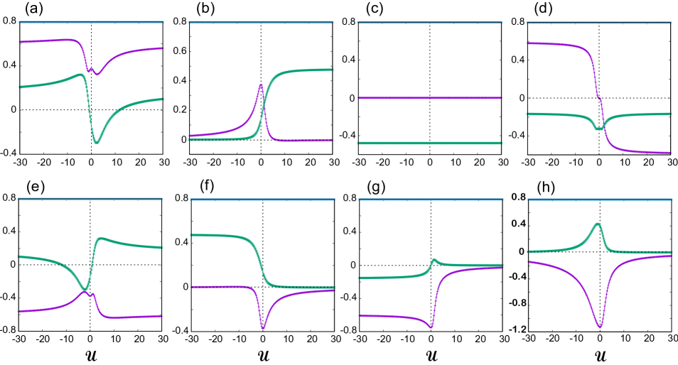
Figure 14: The ${\cal A}$-coefficients (dimensionless) [see Eq. (51)] for the remaining 8 excited eigenstates of 3 bosons trapped in 3 linearly arranged wells as a function of ${\cal U}$ (horizontal axis, dimensionless). This figure complements Fig. 7 in the main text. (a) $i=3r(4l)$. (b) $i=4r(3l)$. (c) $i=5r(6l)$. (d) $i=6r(5l)$. (e) $i=7r(8l)$. (f) $i=8r(7l)$, (g) $i=9$, (h) $i=10$. See text for a detailed description. The choice of online colors is the same as in Fig. 7, that is: ${\cal A}_{0}\rightarrow$ Constant (Light Blue), ${\cal A}_{1}\rightarrow$ Violet, ${\cal A}_{2}\rightarrow$ Green. For the print grayscale version, excluding the top constant ${\cal A}_{0}$ horizontal line, the positioning of the two remaining curves at ${\cal U}=-30$ is as follows: (a,b,c,d) ${\cal A}_{1}\rightarrow$ upper curve, ${\cal A}_{2}\rightarrow$ lower curve. (e,f,g,h) ${\cal A}_{1}\rightarrow$ lower curve, ${\cal A}_{2}\rightarrow$ upper curve.

Appendix G First-order momentum correlations as a function of ${\cal U}$ for the remaining eight excited states

Fig. 14 complements Fig. 7 in that it displays the 3 distinct coefficients ${\cal A}^{i}({\cal U})$’s for the remaining eight excited states (explicit numerical values can be found in the supplemental material supp ). The dependence of these coefficients on the interaction strength ${\cal U}$ is better deciphered by using as reference points the special cases at ${\cal U}\rightarrow\pm\infty$ and ${\cal U}=0$. Note that in all cases the ${\cal B}^{i}$ values at the end points ${\cal U}=\pm 30$ in the figure are close to the corresponding limiting values at ${\cal U}\rightarrow\pm\infty$. In particular,

The excited state denoted as $i=3r(4l)$ ($i=3$ for $0<{\cal U}<+\infty$ and $i=4$ for $-\infty<{\cal U}<0$): For ${\cal U}\rightarrow-\infty$, all 3 cosinusoidal terms survive in expression (51) [see frame (a) in Fig. 14]; specifically one has: ${\cal A}^{4,-\infty}_{0}=0.797885=\sqrt{2/\pi}$, ${\cal A}^{4,-\infty}_{1}=\sqrt{10}/(3\sqrt{\pi})$, and ${\cal A}^{4,-\infty}_{2}=\sqrt{2}/(5\sqrt{\pi})$.

For the non-interacting case (${\cal U}=0$), all 3 coefficients survive in expression (51) [see frame (a) in Fig. 14]; specifically one has: ${\cal A}^{3r(4l),{\cal U}=0}_{0}=0.797885=\sqrt{2/\pi}$, ${\cal A}^{3r(4l),{\cal U}=0}_{1}=0.376126$, and ${\cal A}^{3r(4l),{\cal U}=0}_{2}=-0.140078$.

For ${\cal U}\rightarrow+\infty$, all 3 cosinusoidal terms survive in expression (51) [see frame (a) in Fig. 14]; specifically one has: ${\cal A}^{3,+\infty}_{0}=0.797885=\sqrt{2/\pi}$, ${\cal A}^{3,+\infty}_{1}=\sqrt{10}/(3\sqrt{\pi})$, and ${\cal A}^{3,+\infty}_{2}=\sqrt{2}/(5\sqrt{\pi})$.

The excited state denoted as $i=4r(3l)$ ($i=4$ for $0<{\cal U}<+\infty$ and $i=3$ for $-\infty<{\cal U}<0$): For ${\cal U}\rightarrow-\infty$, only 1 cosinusoidal term survives in expression (51) [see frame (b) in Fig. 14]; specifically one has: ${\cal A}^{3,-\infty}_{0}=0.797885=\sqrt{2/\pi}$, ${\cal A}^{3,-\infty}_{1}=0$, and ${\cal A}^{3,-\infty}_{2}=0$.

For the non-interacting case (${\cal U}=0$), all 3 coefficients survive in expression (51) [see frame (b) in Fig. 14]; specifically one has: ${\cal A}^{4r(3l),{\cal U}=0}_{0}=0.797885=\sqrt{2/\pi}$, ${\cal A}^{4r(3l),{\cal U}=0}_{1}=0.376126$, and ${\cal A}^{4r(3l),{\cal U}=0}_{2}=0.140078$.

For ${\cal U}\rightarrow+\infty$, 2 cosinusoidal terms survive in expression (51) [see frame (b) in Fig. 14]; specifically one has: ${\cal A}^{4,+\infty}_{0}=0.797885=\sqrt{2/\pi}$, ${\cal A}^{4,+\infty}_{1}=0$, and ${\cal A}^{4,+\infty}_{2}=3\sqrt{2}/(5\sqrt{\pi})$.

The excited state denoted as $i=5r(6l)$ ($i=5$ for $0<{\cal U}<+\infty$ and $i=6$ for $-\infty<{\cal U}<0$): This state is ${\cal U}$-independent; see first expression in Eq. (69) or second expression in Eq. (70). In this case, 2 distinct coefficients (corresponding to 2 cosinusoidal terms) survive in expression (51), that is, ${\cal A}^{5,+\infty}_{0}={\cal A}^{6,-\infty}_{0}=\sqrt{2/\pi}={\cal A}^{5r(6l),{\cal U}=0}_{0}=0.797885$, ${\cal A}^{5,+\infty}_{1}={\cal A}^{6,-\infty}_{1}={\cal A}^{5r(6l),{\cal U}=0}_{1}=0$, and ${\cal A}^{5,+\infty}_{2}={\cal A}^{6,-\infty}_{2}={\cal A}^{5r(6l),{\cal U}=0}_{2}=-3\sqrt{2}/(5\sqrt{\pi})$; see frame (c) in Fig. 14.

The excited state denoted as $i=6r(5l)$ ($i=6$ for $0<{\cal U}<+\infty$ and $i=5$ for $-\infty<{\cal U}<0$): For ${\cal U}\rightarrow-\infty$, all 3 cosinusoidal terms survive in expression (51) [see frame (d) in Fig. 14]; specifically one has: ${\cal A}^{5,-\infty}_{0}=0.797885=\sqrt{2/\pi}$, ${\cal A}^{5,-\infty}_{1}=\sqrt{10}/(3\sqrt{\pi})$, and ${\cal A}^{5,-\infty}_{2}=-\sqrt{2}/(5\sqrt{\pi})$.

For the non-interacting case (${\cal U}=0$), 2 coefficients are present in expression (51) [see frame (d) in Fig. 14]; specifically one has: ${\cal A}^{6r(5l),{\cal U}=0}_{0}=0.797885=\sqrt{2/\pi}$, ${\cal A}^{6r(5l),{\cal U}=0}_{1}=0$, and ${\cal A}^{6r(5l),{\cal U}=0}_{2}=-2\sqrt{2}/(5\sqrt{\pi})$.

For ${\cal U}\rightarrow+\infty$, all 3 cosinusoidal terms survive in expression (51) [see frame (d) in Fig. 14]; specifically one has: ${\cal A}^{6,+\infty}_{0}=0.797885=\sqrt{2/\pi}$, ${\cal A}^{6,+\infty}_{1}=-\sqrt{10}/(3\sqrt{\pi})$, and ${\cal A}^{6,+\infty}_{2}=-\sqrt{2}/(5\sqrt{\pi})$.

The excited state denoted as $i=7r(8l)$ ($i=7$ for $0<{\cal U}<+\infty$ and $i=8$ for $-\infty<{\cal U}<0$): For ${\cal U}\rightarrow-\infty$, all 3 cosinusoidal terms survive in expression (51) [see frame (e) in Fig. 14]; specifically one has: ${\cal A}^{8,-\infty}_{0}=0.797885=\sqrt{2/\pi}$, ${\cal A}^{8,-\infty}_{1}=-\sqrt{10}/(3\sqrt{\pi})$, and ${\cal A}^{8,-\infty}_{2}=\sqrt{2}/(5\sqrt{\pi})$.

For the non-interacting case (${\cal U}=0$), all 3 coefficients are present in expression (51) [see frame (e) in Fig. 14]; specifically one has: ${\cal A}^{7r(8l),{\cal U}=0}_{0}=0.797885=\sqrt{2/\pi}$, ${\cal A}^{7r(8l),{\cal U}=0}_{1}=-0.376126$, and ${\cal A}^{7r(8l),{\cal U}=0}_{2}=-0.140078$.

For ${\cal U}\rightarrow+\infty$, all 3 cosinusoidal terms survive in expression (51) [see frame (e) in Fig. 14]; specifically one has: ${\cal A}^{7,+\infty}_{0}=0.797885=\sqrt{2/\pi}$, ${\cal A}^{7,+\infty}_{1}=-\sqrt{10}/(3\sqrt{\pi})$, and ${\cal A}^{7,+\infty}_{2}=\sqrt{2}/(5\sqrt{\pi})$.

The excited state denoted as $i=8r(7l)$ ($i=8$ for $0<{\cal U}<+\infty$ and $i=7$ for $-\infty<{\cal U}<0$): For ${\cal U}\rightarrow-\infty$, 2 cosinusoidal terms are present in expression (51) [see frame (f) in Fig. 14]; specifically one has: ${\cal A}^{7,-\infty}_{0}=0.797885=\sqrt{2/\pi}$, ${\cal A}^{7,-\infty}_{1}=0$, and ${\cal A}^{7,-\infty}_{2}=3\sqrt{2}/(5\sqrt{\pi})$.

For the non-interacting case (${\cal U}=0$), all 3 coefficients are present in expression (51) [see frame (f) in Fig. 14]; specifically one has: ${\cal A}^{8r(7l),{\cal U}=0}_{0}=0.797885=\sqrt{2/\pi}$, ${\cal A}^{8r(7l),{\cal U}=0}_{1}=-0.376126$, and ${\cal A}^{8r(7l),{\cal U}=0}_{2}=0.140078$.

For ${\cal U}\rightarrow+\infty$, only the ${\cal U}$-independent term survives in expression (51) [see frame (f) in Fig. 14]; specifically one has: ${\cal A}^{8,+\infty}_{0}=0.797885=\sqrt{2/\pi}$, ${\cal A}^{8,+\infty}_{1}=0$, and ${\cal A}^{8,+\infty}_{2}=0$.

The excited state denoted as $i=9$ for $-\infty<{\cal U}<+\infty$: For ${\cal U}\rightarrow-\infty$, all 3 cosinusoidal terms are present in expression (51) [see frame (g) in Fig. 14]; specifically one has: ${\cal A}^{9,-\infty}_{0}=0.797885=\sqrt{2/\pi}$, ${\cal A}^{9,-\infty}_{1}=-\sqrt{10}/(3\sqrt{\pi})$, and ${\cal A}^{9,-\infty}_{2}=-\sqrt{2}/(5\sqrt{\pi})$.

For the non-interacting case (${\cal U}=0$), 2 coefficients are present in expression (51) [see frame (g) in Fig. 14]; specifically one has: ${\cal A}^{9,{\cal U}=0}_{0}=0.797885=\sqrt{2/\pi}$, ${\cal A}^{9,{\cal U}=0}_{1}=-4/(3\sqrt{\pi})$, and ${\cal A}^{9,{\cal U}=0}_{2}=0$.

For ${\cal U}\rightarrow+\infty$, only the ${\cal U}$-independent term survives in expression (51) [see frame (g) in Fig. 14]; specifically one has: ${\cal A}^{9,+\infty}_{0}=0.797885=\sqrt{2/\pi}$, ${\cal A}^{9,+\infty}_{1}=0$, and ${\cal A}^{9,+\infty}_{2}=0$.

The excited state denoted as $i=10$ for $-\infty<{\cal U}<+\infty$: For ${\cal U}\rightarrow-\infty$, only the ${\cal U}$-independent term is present in expression (51) [see frame (h) in Fig. 14]; specifically one has: ${\cal A}^{10,-\infty}_{0}=0.797885=\sqrt{2/\pi}$, ${\cal A}^{10,-\infty}_{1}=0$, and ${\cal A}^{10,-\infty}_{2}=0$.

For the non-interacting case (${\cal U}=0$), all 3 coefficients are present in expression (51) [see frame (h) in Fig. 14]; specifically one has: ${\cal A}^{10,{\cal U}=0}_{0}=0.797885=\sqrt{2/\pi}$, ${\cal A}^{10,{\cal U}=0}_{1}=-2/\sqrt{\pi}$, and ${\cal A}^{10,{\cal U}=0}_{2}=1/\sqrt{2\pi}$.

For ${\cal U}\rightarrow+\infty$, only the ${\cal U}$-independent term survives in expression (51) [see frame (h) in Fig. 14]; specifically one has: ${\cal A}^{10,+\infty}_{0}=0.797885=\sqrt{2/\pi}$, ${\cal A}^{10,+\infty}_{1}=0$, and ${\cal A}^{10,+\infty}_{2}=0$.

References

- (1) J. I. Cirac and P. Zoller, Goals and Opportunities in Quantum Simulation, Nat. Phys. 8, 264 (2012).
- (2) M. A. García-March, B. Juliá-Díaz, G. E. Astrakharchik, Th. Busch, J. Boronat and A. Polls, Quantum correlations and spatial localization in one-dimensional ultracold bosonic mixtures, New J. Phys. 16, 103004 (2014).
- (3) J. H. Becher, E. Sindici, R. Klemt, S. Jochim, A. J. Daley, Ph. M. Preiss, Measurement of Identical Particle Entanglement and the Influence of Antisymmetrisation, arXiv:2002.11207.
- (4) P. M. Preiss, J. H. Becher, R. Klemt, V. Klinkhamer, A. Bergschneider, and S. Jochim, High-Contrast Interference of Ultracold Fermions, Phys. Rev. Lett. 122, 143602 (2019).
- (5) A. Bergschneider, V. M. Klinkhamer, J. H. Becher, R. Klemt, L. Palm, G. Zürn, S. Jochim, and P. M. Preiss, Experimental characterization of two-particle entanglement through position and momentum correlations, Nat. Phys. 15, 640 (2019).
- (6) M. Greiner, O. Mandel, T. Esslinger, Th. W. Hänsch, and I. Bloch, Quantum phase transition from a superfluid to a Mott insulator in a gas of ultracold atoms, Nature 415, 39 (2002).
- (7) F. Gerbier, A. Widera, S. Fölling, O. Mandel, T. Gericke, and I. Bloch, Phase Coherence of an Atomic Mott Insulator, Phys. Rev. Lett. 95, 050404 (2005).
- (8) F. Gerbier, A. Widera, S. Fölling, O. Mandel, T. Gericke, and I. Bloch, Interference pattern and visibility of a Mott insulator, Phys. Rev. A 72, 053606 (2005).
- (9) H. Cayla, C. Carcy, Q. Bouton, R. Chang, G. Carleo, M. Mancini, D. Clément, Single-atom-resolved probing of lattice gases in momentum space, Phys. Rev. A 97 061609(R) (2018).
- (10) C. Carcy, H. Cayla, A. Tenart, A. Aspect, M. Mancini, and D. Clément, Momentum-space atom correlations in a Mott insulator, Phys. Rev. X 9, 041028 (2019).
- (11) S. S. Hodgman, R. I. Khakimov, R. J. Lewis-Swan, A. G. Truscott, and K. V. Kheruntsyan, Solving the Quantum Many-Body Problem via Correlations Measured with a Momentum Microscope, Phys. Rev. Lett. 118, 240402 (2017).
- (12) H. Ott, Single atom detection in ultracold quantum gases: A review of current progress, Rep. Prog. Phys. 79, 054401 (2016).
- (13) B. B. Brandt, C. Yannouleas, and U. Landman, Two-point momentum correlations of few ultracold quasi-one-dimensional trapped fermions: Diffraction patterns, Phys. Rev. A 96, 053632 (2017).
- (14) B. B. Brandt, C. Yannouleas, and U. Landman, Interatomic interaction effects on second-order momentum correlations and Hong-Ou-Mandel interference of double-well-trapped ultracold fermionic atoms, Phys. Rev. A 97, 053601 (2018)
- (15) C. Yannouleas, B. B. Brandt, and U. Landman, Interference, spectral momentum correlations, entanglement, and Bell inequality for a trapped interacting ultracold atomic dimer: Analogies with biphoton interferometry, Phys. Rev. A 99, 013616 (2019).
- (16) C. Yannouleas and U. Landman, Anyon optics with time-of-flight two-particle interference of double-well-trapped interacting ultracold atoms, Phys. Rev. A 100, 013605 (2019).
- (17) S. Murmann, A. Bergschneider, V. M. Klinkhamer, G. Zürn, T. Lompe, and S. Jochim, Two fermions in a double well: Exploring a fundamental building block of the Hubbard model, Phys. Rev. Lett. 114, 080402 (2015).
- (18) D. Bouwmeester, J.-W. Pan, M. Daniell, H. Weinfurter, and A. Zeilinger, Observation of Three-Photon Greenberger-Horne-Zeilinger Entanglement, Phys. Rev. Lett. 82, 1345 (1999).
- (19) W. Dür, G. Vidal, and J. I. Cirac, Three qubits can be entangled in two inequivalent ways, Phys. Rev. A 62, 062314 (2000).
- (20) C. Yannouleas and U. Landman, Third-order momentum correlation interferometry maps for entangled quantal states of three singly trapped massive ultracold fermions, Phys. Rev. A 100, 023618 (2019).
- (21) A. Gallemí, M. Guilleumas, J. Martorell1, R. Mayol, A. Polls, and B. Juliá-Díaz, Fragmented condensation in Bose-Hubbard trimers with tunable tunnelling, New J. Phys. 17, 073014 (2015).
- (22) D. Raventós, T. Graß, M. Lewenstein, and B. Juliá-Díaz, Cold bosons in optical lattices: a tutorial for exact diagonalization, J. Phys. B: At. Mol. Opt. Phys. 50, 113001 (2017).
- (23) H. Shiba and P. A. Pincus, Thermodynamic Properties of the One-Dimensional Half-Filled-Band Hubbard Model, Phys. Rev. B 5, 1966 (1972).
- (24) J. Callaway, D. P. Chen, and R. Tang, Ground-state and thermodynamic properties of the Hubbard model applied to small clusters, Phys. Rev. B 35, 3705 (1987).
- (25) E. Dagotto, Correlated electrons in high-temperature superconductors, Rev. Mod. Phys. 66, 763 (1994).
- (26) A. M. Kaufman, B. J. Lester, C. M. Reynolds, M. L. Wall, M. Foss-Feig, K. R. A. Hazzard, A. M. Rey, and C. A. Regal, Two-particle quantum interference in tunnel-coupled optical tweezers, Science 345, 306 (2014).
- (27) A. M. Kaufman, M. C. Tichy, F. Mintert, A. M. Rey, and C. A. Regal, The Hong-Ou-Mandel Effect With Atoms, in Atomic, Molecular, and Optical Physics 67, 377 (2018).
- (28) D. Peçak and T. Sowínski, Few strongly interacting ultracold fermions in one-dimensional traps of different shapes, Phys. Rev. A 94, 042118 (2016); T. Plaßmann, S. I. Mistakidis, and P. Schmelcher, Quench dynamics of finite bosonic ensembles in optical lattices with spatially modulated interactions, J. Phys. B: At. Mol. Opt. Phys. 51, 225001 (2018).
- (29) A. G. Volosniev, D. V. Fedorov, A. S. Jensen, N. T. Zinner, and M. Valiente, Multicomponent Strongly Interacting Few-Fermion Systems in One Dimension, Few-Body Systems 55, 839 (2014).
- (30) The algebraic scripts for the formulas presented in this paper can be obtained from the authors upon request.
- (31) In a finite system there are no sharp phase transitions associated with symmetry breaking. Our solutions of the Hubbard trimer are exact (they do not break any symmetries of the Hamiltonian). Accordingly, we use here the terminology “signatures of emergent phase transitions.” This terminology is used in the literature of finite systems [see, e.g., T. Papenbrock and H. A. Weidenmüller, Effective field theory of emergent symmetry breaking in deformed atomic nuclei, J. Phys. G: Nucl. Part. Phys. 42, 105103 (2015)] to indicate that symmetry breaking and the sharp phase transitions emerge gradually from the behavior of finite systems in the limit of . We choose here this terminology over an alternative one, namely ’phase-crossover’ that is used in some cases to discuss the broad phase-related changes in finite systems.
- (32) K. Sengupta and N. Dupuis, Mott-insulator-to-superfluid transition in the Bose-Hubbard model: A strong-coupling approach, Phys. Rev. A 71, 033629 (2005).
- (33) J. K. Freericks, H. R. Krishnamurthy, Y. Kato, N. Kawashima, and N. Trivedi, Strong-coupling expansion for the momentum distribution of the Bose-Hubbard model with benchmarking against exact numerical results, Phys. Rev. A 79, 053631 (2009).
- (34) T. Legero, T. Wilk, M. Hennrich, G. Rempe, and A. Kuhn, Quantum Beat of Two Single Photons, Phys. Rev. Lett. 93, 070503 (2004).
- (35) T. Gerrits, F. Marsili, V. B. Verma, L. K. Shalm, M. Shaw, R. P. Mirin, and S. W. Nam, Spectral correlation measurements at the Hong-Ou-Mandel interference dip, Phys. Rev. A 91, 013830 (2015).
- (36) R.-B. Jin, T. Gerrits, M. Fujiwara, R. Wakabayashi, T. Yamashita, S. Miki, H. Terai, R. Shimizu, M. Takeoka, and M. Sasaki, Spectrally resolved Hong-Ou-Mandel interference between independent photon sources, Opt. Express 23, 28836 (2015).
- (37) X.-J. Wang, B. Jing, P.-F. Sun, C.-W. Yang, Y. Yu, V. Tamma, X.-H. Bao, and J.-W. Pan, Experimental Time-Resolved Interference with Multiple Photons of Different Colors, Phys. Rev. Lett. 121, 080501 (2018).
- (38) V. V. Orre, E. A. Goldschmidt, V. Tamma, M. Hafezi, and S. Mittal, Interference of multiple temporally distinguishable photons using frequency-resolved detection, Phys. Rev. Lett. 123, 123603 (2019).
- (39) M. Bonneau, W. J. Munro, K. Nemoto, and J. Schmiedmayer, Characterizing twin-particle entanglement in double-well potentials, Phys. Rev. A bf 98, 033608 (2018).
- (40) S. Laibacher and V. Tamma, Symmetries and entanglement features of inner-mode-resolved correlations of interfering nonidentical photons, Phys. Rev. A 98, 053829 (2018).
- (41) C. K. Hong, Z. Y. Ou, and L. Mandel, Measurement of subpicosecond time intervals between two photons by interference, Phys. Rev. Lett. 59, 2044 (1987).
- (42) R. C. Liu, B. Odom, Y. Yamamoto, and S. Tarucha, Quantum interference in electron collision, Nature (London) 391, 263 (1998).
- (43) T. Jonckheere, J. Rech, C. Wahl, and T. Martin, Electron and hole Hong-Ou-Mandel interferometry, Phys. Rev. B 86, 125425 (2012).
- (44) E. Bocquillon, V. Freulon, J.-M. Berroir, P. Degiovanni, B. Plaçais, A. Cavanna, Y. Jin, and G. Fève, Coherence and indistinguishability of single electrons emitted by independent sources, Science 339, 1054 (2013).
- (45) R. Lopes, A. Imanaliev, A. Aspect, M. Cheneau, D. Boiron, and C. I. Westbrook, Atomic Hong-Ou-Mandel experiment, Nature (London) 520, 66 (2015).
- (46) See, e.g., Ref. prei19 for a first experimental realization of such a TOF spectroscopy in the case of 3 trapped fully spin-polarized ultracold fermions.
- (47) S. Mährlein, J. von Zanthier, and G.S. Agarwal, Complete three photon Hong-Ou-Mandel interference at a three port device, Optics Express 23, 15833 (2015).
- (48) S. Agne, Th. Kauten, J. Jin, E. Meyer-Scott, J. Z. Salvail, D. R. Hamel, K. J. Resch, G. Weihs, and Th. Jennewein, Observation of Genuine Three-Photon Interference, Phys. Rev. Lett. 118, 153602 (2017).
- (49) A. J. Menssen, A. E. Jones, B. J. Metcalf, C. Tichy, S. Barz, W. S. Kolthammer, and I. A. Walmsley, Distinguishability and Many-Particle Interference, Phys. Rev. Lett. 118, 153603 (2017).
- (50) S. Aaronson and A. Arkhipov, The computational complexity of linear optics, Theory Comput. 9 143 (2013).
- (51) M.C. Tichy, Interference of identical particles from entanglement to boson-sampling, J. Phys. B: At. Mol. Opt. Phys. 47, 103001 (2014).
- (52) V. Tamma and S. Laibacher, Multiboson Correlation Interferometry with Arbitrary Single-Photon Pure States, Phys. Rev. Lett. 114, 243601 (2015).
- (53) S. Laibacher and V. Tamma, From the Physics to the Computational Complexity of Multiboson Correlation Interference, Phys. Rev. Lett. 115, 243605 (2015).
- (54) J. Carolan, J. D. A. Meinecke, P. J. Shadbolt, N. J. Russell, N. Ismail, K. Wörhoff, T. Rudolph, M. G. Thompson, J. L. O’Brien, J. C. F. Matthews, and A. Laing, On the experimental verification of quantum complexity in linear optics, Nature Photonics 8, 621 (2014).
- (55) M. Walschaers, Signatures of many-particle interference, J. Phys. B: Atom. Mol. Opt. 53, 043001, (2020).
- (56) R. Zitko, SNEG - Mathematica package for symbolic calculations with second-quantization-operator expressions, Comp. Phys. Comm. 182, 2259 (2011).
- (57) Wolfram Research, Inc., Mathematica, Version 11.3, Champaign, IL (2018).
- (58) P.-O. Löwdin, Quantum theory of many-particle systems. I. Physical interpretations by means of density matrices, natural spin-orbitals, and convergence problems in the method of configurational interaction, Phys. Rev. 97, 1474 (1955).
- (59) M. Alvioli, C. Cio degli Atti, L. P. Kaptari, C. B. Mezzetti, H. Morita, and S. Scopetta, Universality of nucleon-nucleon short-range correlations: Two-nucleon momentum distributions in few-body systems, Phys. Rev. C 85, 021001(R) (2012).
- (60) C. A. Coulson, Momentum Distribution in Molecular Systems: Part I. The Single Bond, Proc. Cambridge Phil. Soc. 37, 55 (1941).
- (61) A. Szabo and N.S. Ostlund, Modern Quantum Chemistry: Introduction to Advanced Electronic Structure Theory, Revised first edition (McGraw-Hill, New York, 1989).
- (62) https://en.wikipedia.org/wiki/Linear_combination_of_atomic_orbitals
- (63) https://mathworld.wolfram.com/FourierTransform.html
- (64) The multiwell confining spatial potential, used in conjunction with full configuration interaction (CI) microscopic calculations, has been extensively described in the Supplemental Information section of B. B. Brandt, C. Yannouleas, and U. Landman, Double-Well Ultracold-Fermions Computational Microscopy: Wave-Function Anatomy of Attractive-Pairing and Wigner-Molecule Entanglement and Natural Orbitals, Nano Lett. 15, 7105 (2015), and in C. Yannouleas, B. B. Brandt, and U, Landman, Ultracold few fermionic atoms in needle-shaped double wells: spin chains and resonating spin clusters from microscopic Hamiltonians emulated via antiferromagnetic Heisenberg and - models, New J. Phys. 18, 073018 (2016), as well as in Ying Li, C. Yannouleas, and U. Landman, Artificial quantum-dot helium molecules: Electronic spectra, spin structures, and Heisenberg clusters Phys. Rev. B 80, 045326 (2009).
- (65) By controlling the potential barrier and the distance between the wells, small overlaps of the localized atomic orbitals (which guarantee the validity of our augmented Hubbard model also in the range of small values of ) are purposefully and routinely realized in current experiments with optical tweezers, see, e.g., S. Murmann, A. Bergschneider, V. M. Klinkhamer, G. Zürn, Th. Lompe, and S. Jochim, Two Fermions in a Double Well: Exploring a Fundamental Building Block of the Hubbard Model, Phys. Rev. Lett. 114, 080402 (2015), and A. M. Kaufman, B. J. Lester, C. M. Reynolds, M. L. Wall, M. Foss-Feig, K. R. A. Hazzard, A. M. Rey, and C. A. Regal, Two-particle quantum interference in tunnel-coupled optical tweezers, Science 345, 306 (2014).
- (66) Extensive comparisons between the full CI momentum correlations and those from the augmented Hubbard model have been carried out in Refs. bran17 and bran18 for double, triple, and quadruple wells. Recently available experimentally measured momentum correlation maps berg19 for double wells show an excellent agreement with the theoretical results in the full range .
- (67) Supplemental material …
- (68) T. Young, I. The Bakerian Lecture. Experiments and calculations relative to physical optics, Phil. Trans. R. Soc. London 94, 1 (1804).
- (69) S. Fölling, F. Gerbier, A. Widera, O. Mandel, T. Gericke, and I. Bloch, Spatial quantum noise interferometry in expanding ultracold atom clouds, Nature 434, 491 (2005).
- (70) M. P. A. Fisher, P. B. Weichman, G. Grinstein, and D. S. Fisher, Boson localization and the superfluid-insulator transition, Phys. Rev. B 40, 546 (1989).
- (71) For a clear description of this contribution, see Eq. (11) and related text in Ref. gerb05.2 .
- (72) C. Yannouleas and U. Landman (unpublished).
- (73) Z. Y. Ou, Multi-Photon Quantum Interference (Springer, New York, 2007).
- (74) Y. H. Shih, An Introduction to Quantum Optics: Photon and Biphoton Physics (CRC Press, Boca Raton, FL, 2011).
- (75) X. Lu and Y. Yu, Finite-temperature effects on the number fluctuation of ultracold atoms across the superfluid-to-Mott-insulator transition, Phys. Rev. A 74, 063615 (2006).
- (76) S. Jin, X. Guo, P. Peng, X. Chen, X. L, and X. Zhou, Finite temperature phase transition in a cross-dimensional triangular lattice, New J. Phys. 21, 073015 (2019).
- (77) N. Spagnolo, C. Vitelli, L. Aparo, P. Mataloni, F. Sciarrino, A. Crespi, R. Ramponi, and R. Osellame, Three-photon bosonic coalescence in an integrated tritter, Nat. Commun. 4, 1606 (2013).
- (78) A tritter is a device of 3 parallel optical fibers that are brought closer at a point and then are separated again; see the schematic in Fig. 1(b) in Ref. spag13 and in Fig. 5 of G. Weihs, M. Reck, H. Weinfurter, and A. Zeilinger, Two-photon interference in optical fiber multiports, Phys. Rev. A 54, 893 (1996).
- (79) It also applies for the case of a few strongly entangled fermions yann19.3 .
- (80) J. V. Gomes, A. Perrin, M. Schellekens, D. Boiron, C. I. Westbrook, and M. Belsley, Theory for a Hanbury Brown Twiss experiment with a ballistically expanding cloud of cold atoms, Phys. Rev. A 74, 053607 (2006).
- (81) R. G. Dall, A. G. Manning, S. S. Hodgman, W. Rugway, K. V. Kheruntsyan, and A. G. Truscott, Ideal -body correlations with massive particles, Nature Phys. 9, 341 (2013).
- (82) T. Schweigler, V. Kasper, S. Erne, I. Mazets, B. Rauer, F. Cataldini, T. Langen, T. Gasenzer, J. Berges, and J. Schmiedmayer, Experimental characterization of a quantum many-body system via higher-order correlations, Nature 545, 323 (2017).