Experimental and modelling evidence for structural crossover in supercritical CO₂

Abstract

Physics of supercritical state is understood to a much lesser degree compared to subcritical liquids. Carbon dioxide in particular has been intensely studied, yet little is known about the supercritical part of its phase diagram. Here, we combine neutron scattering experiments and molecular dynamics simulations and demonstrate the structural crossover at the Frenkel line. The crossover is seen at pressures as high as 14 times the critical pressure and is evidenced by changes of the main features of the structure factor and pair distribution functions.

Usage

Secondary publications and information retrieval purposes.

PACS numbers

May be entered using the \pacs{#1} command.

I Introduction

Supercritical fluids have unique properties that have led to a rich variety of applications deben . Rare gases, nitrogen, CO₂ and H₂O are among the most common supercritical fluids. CO₂ in particular is an important greenhouse gas of Earth’s atmosphere, and in its supercritical state is the main component (97%) in the atmosphere of Venus. Supercritical CO₂ is used in a great variety of applications (see, e.g., applications in solubility, synthesis and processing of polymers co9 ; co13 ; co11 , dissolving and deposition in microdevices co7 , green chemistry and solvation co6 ; co4 ; co1 ; co3 ; co10 ; co15 ; co16 , green catalysis co17 ; co3 ; co2 ; co51 , extraction co5 , chemical reactions co8 , green nanosynthesis co12 and sustainable development including carbon capture and storage co14 ). It has been widely appreciated that improving fundamental knowledge of the supercritical state is important for the reliability, scale-up and widening of these applications (see, e.g., Refs deben ; co3 ; co4 ; co51 ; co8 ; co16 ).

Compared to subcritical liquids, the supercritical state is not well understood. Traditional understanding amounted to a general assertion that this state is physically homogeneous, with no qualitative changes taking place anywhere above the critical point deben . The first challenge to this view was the Widom Line (WL). Close to the critical point, the WL characterises persisting near-critical anomalies such as the maximum in the heat capacity stanleywidom05 , which can be used to stratify different states in the supercritical region. A different subsequent proposal was based on the Frenkel line (FL) separating two distinct states in the supercritical state with liquid-like and gas-like dynamics. Differently from the WL, the FL extends to arbitrarily high pressures and temperatures (as long as chemical bonding is unaltered), is unrelated to the critical point and exists in systems with no boiling line or critical point pre ; prl ; phystoday . The FL is also of practical importance because it corresponds to the solubility maxima in supercritical CO₂ pre1 .

Here, we combine neutron scattering experiments and molecular dynamics (MD) simulations and show evidence for the structural crossover of supercritical carbon dioxide at the Frenkel line. The crossover extends to pressure as high as 14 times the critical pressure and is evidenced by changes of the main features of the structure factor and pair distribution functions. The neutron scattering experiments evidencing a crossover at highly supercritical pressure are the first of its kind for CO₂.

II Methods

We recall that particle dynamics combine solid-like oscillations around quasi-equilibrium positions and diffusive jumps between different positions below the FL, the typical character of molecular motion in liquids frenkel . Above the line, particle dynamics lose this oscillatory component and become purely diffusive. This gives a practical criterion to calculate the FL based on the disappearance of minima of the velocity autocorrelation function (VAF) prl . This criterion coincides with the thermodynamic criterion $c_{v}=2k_{\rm B}$ corresponding to the disappearance of transverse-like excitations in a monatomic system ropp . Since structure and dynamics are related argon , the FL crossover was predicted to result in a crossover of the supercritical structure.

The pressures we consider for both experiments and MD simulations are 500 and 590 bar. The FL in CO₂ was previously calculated using the VAF criterion pre1 , giving us the following two state points of the predicted crossover: (500 bar, 297 K) and (590 bar, 302 K). We recall that the FL extends to arbitrarily high pressure and temperature above the critical point, but at low temperature it touches the boiling line at around 0.8$T_{c}$, where $T_{c}$ is the critical temperature prl (note that the system does not have cohesive liquid-like states at temperatures above approximately 0.8$T_{c}$ stishov , hence crossing the boiling line at around $0.8T_{c}$ and above can be viewed as a gas-gas transition prl .) The critical point of CO₂ is (73.9 bar, 304.3 K), hence our state points correspond to near-critical temperatures and pressures well above critical. In this regard, we note that the supercritical state is often defined as the state at $P>P_{c}$ and $T>T_{c}$. This definition is loose, not least because an isotherm drawn on ($P$, $T$) diagram above the critical point crosses the melting line, implying that the supercritical state can be found in the solid phase. As a result, one can meaningfully speak about near-critical part of the phase diagram only when discussing the location of the supercritical state on the phase diagram uspehi . As far as our state points are concerned, they correspond to temperatures much higher than the melting temperature and pressures extending to 14 times the critical pressure where near-critical anomalies are non-existent uspehi .

A cylinder of carbon dioxide was obtained from BOC, CP grade, and used without further purification. The pressure of the cylinder was around 50 bar and a SITEC intensifier and a SITEC hand pump gas was used to raise the pressure. Capillaries were used to connect intensifier manifold system to the cell. The flat plate pressure cell was made from an alloy of Ti and Zr in the mole ratio 0.676:0.324, which contributes almost zero coherent scattering to the diffraction pattern soper17 . The cell consisted of a flat section that was 12 mm thick and had four 6 mm diameter holes running through it, so the occupied gas space was 6 mm thick and the wall thickness was 3 mm either side. The container was placed at right angle to the neutron beam, which was approximately 30 mm x 30 mm in cross section. A bottom loading closed cycle helium refrigerator was used to control the temperature within $\pm$ 1 K, using He exchange gas at $\sim$20 mbar to provide temperature uniformity. The employed temperatures and pressures are shown in Table 1, where the densities were calculated from the data available in the NIST database nist .

Table 1:  $T-P-d$ state points for neutron scattering measurements. The values of $d$ are taken from nist .

$T_{\rm exp}$ (K)	$P_{\rm exp}$ (bar)	$d$ (g/mL)	$P_{\rm exp}$ (bar)	$d$ (g/mL)
250	500	1.1676	590	1.1821
270	500	1.1131	590	1.1306
290	500	1.0573	590	1.0784
310	500	1.0003	590	1.0257
330	500	0.9426	590	0.9729
340	500	0.9137	-	-
350	500	0.8848	590	0.9204
360	500	0.8560	-	-
370	500	0.8276	590	0.8688
380	500	0.7996	590	0.8436
390	500	0.7722	590	0.8188

Total neutron scattering measurements were performed on the NIMROD diffractometer at the ISIS pulsed neutron source bowron10 . Absolute values of the differential cross sections were obtained from the raw scattering data by normalising the data to the scattering from a slab of vanadium of known thickness, and were further corrected for background and multiple scattering, container scattering and self-attenuation, using the Gudrun data analysis program gudrun . Finally the data were put on absolute scale of barns per atom per sr by dividing by the number of atoms in the neutron beam (1 barn = $10^{-28}\rm{m}^{2}$).

$$F(Q)=\frac{1}{9}b_{\rm C}^{2}H_{\rm CC}(Q)+\frac{4}{9}b_{\rm O}^{2}H_{\rm OO}(Q)+\frac{4}{9}b_{\rm C}b_{\rm O}H_{\rm CO}(Q)$$

(1)

where $b_{\alpha}$ is the neutron scattering length of atom $\alpha$, and the partial structure factor $H_{\alpha\beta}(Q)$ is the three-dimensional Fourier transform of the corresponding site-site radial distribution function:

$$H_{\alpha\beta}(Q)=4\pi\rho\int_{0}^{\infty}r^{2}(g_{\alpha\beta}(r)-1)\frac{\sin Qr}{Qr}dr$$ (2)

and $\rho$ is the atomic number density. Note that the $H_{\rm OO}(Q)$ and $H_{\rm CO}(Q)$ terms include both the intra- and inter-molecular scattering. The results are shown in Fig. 1.

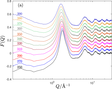
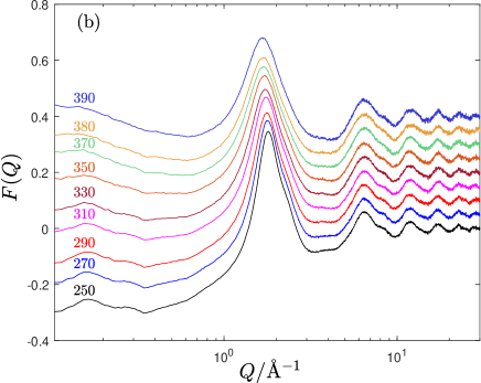
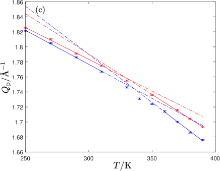
Figure 1: Weighted sum of the experimental weighted partial structure factors $F(Q)$ for CO₂ at (a) 500 bar and (b) 590 bar. The curves for higher temperatures have been shifted along the y-axis by 0.05 per set. (c) Position of the maximum of the first peak in the total (weighted sum) experimental structure factor as a function of temperature for CO₂ at 500 bar (blue) and 590 bar (red). The straight lines are visual guides.

The molecular dynamics (MD) simulation package DL_POLY dlpoly06 was used to simulate a system of 30752 CO₂ particles with periodic boundary conditions. The potential for CO₂ is a rigid-body non-polarizable potential based on a quantum chemistry calculation, with the partial charges derived using the distributed multipole analysis method gao17 . The electrostatic interactions were evaluated using the smooth particle mesh Ewald method in MD simulations. The potential was derived and tuned using a large suite of energies from ab initio density functional theory calculations of different molecular clusters and validated against various sets of experimental data including phonon dispersion curves and $PVT$ data. These data included solid, liquid and gas states, gas-liquid coexistence lines and extended to high-pressure and high-temperature conditions gao17 . We also used another rigid-body non-polarizable potential developed by Zhang and Duan rigidpotential and found the same results.

The MD systems were first equilibrated in the constant pressure and temperature ensemble for 500 ps. The data were subsequently collected from production runs in the constant energy and volume ensemble. In order to reduce noise and see the crossover clearly, data were averaged over 500,000 frames, involving production runs of further 500 ps.

III Results and discussion

Before analyzing the data, we recall that the FL corresponds to the qualitative change of particle dynamics: from combined solid-like oscillatory and diffusive dynamics below the line to purely diffusive gas-like dynamics above the line. Therefore, the supercritical structure is predicted to show the crossover between the liquid-like and gas-like structural correlations. This is predicted to be the case for functions characterizing the structure, such as pair distribution function (PDF) and structure factor (SF). In our analysis, we focus on meaningful features such as maxima positions of PDFs and SFs.

The experimental weighted sum of the partial structure factors are plotted in Fig. 1 for two pressures. We plot the first peaks position of SFs vs temperature in Fig. 1 and observe that it undergoes the crossover at temperatures close to 320 K and around 12% larger than the FL crossover temperature predicted from the VAF criterion mentioned earlier.

The SFs were Fourier transformed to obtain the experimental PDF. As with previous experimental and modelling results on Ar argon , Ne ne , CH₄ methane , and especially on H₂O water pronounced changes of first peak position in the PDF with temperature are observed, indicating a well-defined crossover. When a system is compressed or expanded, one expects the first nearest-neighbour distance, $r_{\mathrm{fnn}}$ (given by the radial position of the first peak in g(r)), and the system’s “length” ($V^{1/3}$) to be proportional to each other unless the system undergoes a structural change. In other words the system structure undergoes uniform compression. The first PDF peak position divided by the position ($r_{0}$) at the Frenkel temperature vs the cube root of the volume divided by the volume ($V_{0}$) at the same reference temperature is shown in Fig. 2. For a system undergoing uniform compression, $V/V_{0}$ and $r/r_{0}$ will be equal. If there is a phase transition at higher densities, as there is in liquids across the melting line, this rule cannot be extrapolated down to arbitrarily low volumes and hence there will be an intercept: $V^{\frac{1}{3}}=\alpha r+\beta$, upon which the gradient of $V/V_{0}$ vs. $r/r_{0}$ will depend. However as long as no structural changes occur, the gradient will remain constant. Specifically, in a simple cubic crystalline solid (atomic packing fraction 0.52) the constant of proportionality between $V/N$ and $r$ is unity, in a FCC lattice (packing fraction 0.74) the constant is 0.89, and in a diamond cubic lattice (packing fraction 0.34), the constant is 1.2. In gases, the fnn distance is largely determined by the size, geometry, and interaction of the constituent molecules (see, e.g., ziman ) rather than the density. This linear relationship has been experimentally observed in molten group 1 elements katayama2 ; katayama3 and liquid CS₂ katayama1 . The fnn distance is most readily extracted from the partial C-C PDFs. The experimental data give the total PDF, but the peak corresponding to the fnn distance is not profoundly changed, therefore the total PDF gives a qualitative approximation of the fnn distance. In Fig. 2 we observe the crossover of the first PDF peak at a temperature within 10% of the predicted crossover temperature at the FL, signified by the change of gradients. This qualitative behaviour is seen more clearly in the MD results (Fig. 4).

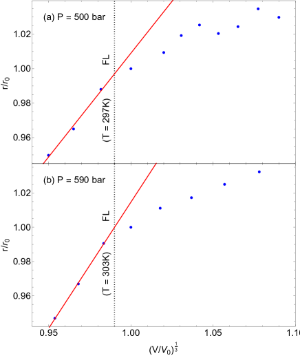
Figure 2: First peak positions of experimental weighted sum PDF for CO₂ at (a) 500 bar and (b) 590 bar as a function of volume. The vertical dashed lines show the reduced volumes at the FL, and the straight lines are visual guides.

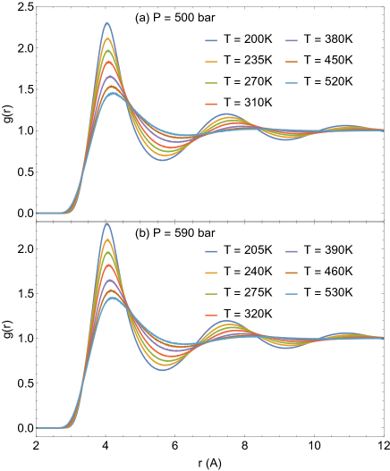
Figure 3: (Colour online) Evolution of the simulated C-C pair distribution functions with temperature at (a) 500 bar and (b) 590 bar.

We now discuss the MD results. Examples of C-C PDFs from MD simulations are shown in Fig. 3. We observe a reduction in height, and corresponding broadening of peaks with increasing temperature as expected. The steepness of the first peak is related with the softness of the effective intermolecular potential, and its reduction can be quantitatively related to the reduction of the viscosity shearline . Fig. 4 displays the radial positions of the first PDF peaks as a function of volume, as discussed above, which shows a crossover at densities near the FL. Because of the reduced noise and abundance of temperature points we can perform statistical analysis of the data to quantify the crossover. We see the same behaviour, including a much clearer crossover, for both pressures. The constant of proportionality between $V/N$ and $r$ is $\approx 3.4$, implying a much more open arrangement than the crystal systems quoted above. This is in accordance with the density of CO₂ at the FL (23346 mol/m³), less than half that of water (56501 mol/m³) at the same pressure and temperature. In order to quantify the crossover, we fitted the data to two different types of function. The first was a single functional dependence over the entire range. In order to avoid the extrapolation errors associated with high order polynomials, the trial functions we used were quadratic, or log plus linear: $f(x)=a+bx+c\log(x)$, with $a$, $b$, and $c$ the fitting parameters. The second set of functions was linear below a certain crossover volume $V_{c}$, and either quadratic or log plus linear above that volume (i.e. a piecewise function): $f(x)=\Theta(V_{c}-V)[a+bx]+\Theta(V-V_{c})[\alpha+\beta x+\gamma\log(x)]$, with $\Theta[V]$ the Heaviside step function and $a$, $b$, $\beta$, $\gamma$, and $V_{c}$ the fitting parameters ($\alpha$ depends on the other parameters in order to ensure continuity of the function).

Generally speaking, adding more parameters to a fitting function improves the numerical quality of the fit. A priori, one can penalise having too many parameters - this prevents the extreme situation of a perfect fit acquired using a piecewise function with a number of subdomains equal to the number of data. The two closely related quantitative measures of goodness of fit with penalty terms for the number of parameters are the AIC (Akaike Information Criterion) AIC and BIC (Bayesian Information Criterion) BIC . Applied to our data, at both pressures and with the quadratic and log plus linear variants, the AIC and BIC were substantially lower than $-10$ below those for the single function, representing a decisive preference for two different functional dependences above and below a certain volume ($V_{c}$). This volume is shown in the vertical dotted line (Fig. 4) and corresponds at both pressures to a temperature close to 350 K, which is within 12-15% of the predicted crossover value. Also plotted as insets in Fig. 4 are the residuals of the low-volume linear fits which show a sharp and sudden increase above the crossover volume, which would not be the case if we had simply interpolated a straight line between non-linear data.

Fig. 5 shows theoretical PDF peak heights. We note that the PDF peak heights of a solid $h=g(r_{\mathrm{peak}})-1$ are predicted tld ; frenkel to have a power-law relationship with temperature, resulting in the following relation: $\log h\propto-\log T$ with $h=g(r)-1$ at the peak. The same relation can be argued to apply to liquids below the FL where the solid-like oscillatory component of molecular motion is present argon . This is because for small displacements the energy is roughly quadratic and the displacement distribution will be Gaussian. The height of a Gaussian distribution follows a power-law relationship with its variance, and thus with temperature. The peak heights in Fig. 5 clearly show the crossover at the FL, with the observed crossover temperatures differing from the predicted ones by about 7-15%. This is in agreement with the width of the FL crossover seen experimentally and modelling on the basis of structural and thermodynamic properties ne ; cv .

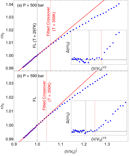
Figure 4: First peak position of simulated C-C PDF. The straight lines are fitted to data below the FL and serve as visual guides. The vertical dashed lines show the fitted crossover volume and the volume at the FL. The insets show the relative trend of the residuals of the linear fit.

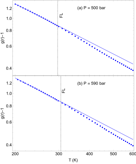
Figure 5: First peak height of C-C PDF for simulated CO₂ at (a) 500 bar and (b) 590 bar as a function of volume. The vertical dashed lines show the temperatures of the predicted crossover, and the solid lines show the fitted straight lines.

Before concluding, we note that previous experiments detecting the structural crossover at the FL involved X-ray scattering in supercritical Ne ne , the combination of X-ray with Raman scattering in supercritical CH₄ methane , and the combination of neutron and Raman scattering in supercritical N₂ n2 . Only one small-angle neutron scattering experiment had been used to study the FL in CO₂ in the vicinity of the critical point only droplet . Our current neutron scattering experiment detecting the crossover at the FL at highly supercritical pressures is the first of its kind and importantly widens the range of techniques used to detect the FL. It will stimulate further neutron scattering experiments in important systems such as supercritical H₂O where a pronounced crossover at the FL was recently predicted on the basis of MD simulations water .

In summary, our combined neutron scattering and molecular dynamics simulations study has detected the structural crossover in CO₂ at pressures well above the critical pressure and temperatures well in excess of melting temperature. The crossover is seen in the main features of the SF and PDFs and corresponds to the predicted crossover at the FL. Apart from the fundamental importance of understanding the supercritical state, the FL corresponds to the solubility maxima of several solutes in supercritical CO₂ pre1 and is therefore of practical importance.

Neutron beam time at ISIS and project funding was provided by the Science and Technology Facilities Council (RB1720056). We acknowledge Chris Goodway, Thomas Headen and Damian Fornalski (Rutherford Appleton Laboratory) for help with the experiments. This research utilized Queen Mary’s MidPlus computational facilities, supported by QMUL Research-IT, http://doi.org/10.5281/zenodo.438045.

References

- (1) E. Kiran, P. G. Debenedetti and C. J. Peters, Supercritical Fluids: Fundamentals and Applications (NATO Science Series E: Applied Sciences vol 366) (Boston: Kluwer, 2000).
- (2) T. Sarbu, T. Styranec and E. J. Beckman, Nature 405, 165 (2000).
- (3) J. M. DeSimone, Z. Guan and C. S. Elsbernd, Science 257, 945 (1992).
- (4) A. I Cooper, J. Mater. Chem. 10, 207 (2000).
- (5) J. M. Blackburn, D. P. Long, A. Cabañas and J. J. Watkins, Science 294, 141 (2001).
- (6) J. M. DeSimone, Science 297, 799 (2002).
- (7) C. A. Eckert, B. L. Knutson and P. G. Debenedetti, Nature 383, 313 (1996).
- (8) C. J. Li and B. M. Trost, PNAS 105, 13197 (2008).
- (9) W. Leitner, Acc. Chem. Res. 35, 746 (2002).
- (10) P. T. Anastas and M. M. Kirchhoff, Acc. Chem. Res. 35, 686 (2002).
- (11) P. Anastas and N. Eghbali, Chem. Soc. Rev. 39, 301 (2010).
- (12) E. J. Beckman, J. Super. Fluids 28, 121 (2004).
- (13) D. J. Cole-Hamilton, Science 299, 1702 (2003).
- (14) P. G. Jessop, Y. Hsiao, T. Ikarita and R. Noyori, J. Am. Chem. Soc. 118, 344 (1996).
- (15) P. G. Jessop, T. Ikariya and R. Noyori, Chem. Rev. 99, 475 (1999).
- (16) E. Reverchon, J. Super. Fluids 10, 1 (1997).
- (17) P. E. Savage, S. Gopalan, T. I. Mizan, C. J. Martino, E. E. Brock, AIChE J. 41, 1723 (1995).
- (18) J. A. Dahl, B. L. S. Maddux and J. E. Hutchison, Chem. Rev. 107, 2228 (2007).
- (19) C. Song, Catalysis Today 115, 2 (2006).
- (20) L. Xu, P. Kumar, S. V. Buldyrev, S.-H. Chen, P. H. Poole, F. Sciortino and H. E. Stanley, PNAS 102, 16558 (2005).
- (21) V. V. Brazhkin, Yu. D. Fomin, A. G. Lyapin, V. N. Ryzhov and K. Trachenko, Phys. Rev. E 85, 031203 (2012).
- (22) V. V. Brazhkin, Yu. D. Fomin, A. G. Lyapin, V. N. Ryzhov, E. N. Tsiok and K. Trachenko, Phys. Rev. Lett. 111, 145901 (2013).
- (23) V. V. Brazhkin and K. Trachenko, Physics Today 65(11), 68 (2012).
- (24) C. Yang, V. V. Brazhkin, M. T. Dove and K. Trachenko, Phys. Rev. E 91, 012112 (2015).
- (25) J. Frenkel, Kinetic Theory of Liquids (New York: Dover 1955).
- (26) K. Trachenko and V. V. Brazhkin, Rep. Prog. Phys. 79, 016502 (2016).
- (27) L. Wang, C. Wang, M. T. Dove, Yu. D. Fomin, V. V. Brazhkin and K. Trachenko, Phys. Rev. E 95 032116 (2017).
- (28) S. M. Stishov, JETP Lett. 57, 196 (1993).
- (29) V. V. Brazhkin, A. G. Lyapin, V. N. Ryzhov, K. Trachenko, Yu. D. Fomin, E. N. Tiosk, Physics Uspekhi 55(11), 1061 (2012).
- (30) A. K. Soper and D. T. Bowron, Chem. Phys. Lett. 683 529-535 (2017).
- (31) National Institute of Standards and Technology database, see https://webbook.nist.gov/chemistry/fluid.
- (32) D. T. Bowron, A. K. Soper, K. Jones, S. Ansell, S. Birch, J. Norris, L. Perrott, D. Riedel, N. J. Rhodes, S. R. Wakefield, A. Botti, M. A. Ricci, F. Grazzi, and M. Zoppi, Rev. Sci. Instrum. 81 33905 (2010).
- (33) A. K. Soper, See http://purl.org/net/epubs/work/56240 (accessed 14 May 2019).
- (34) I. T. Todorov, B. Smith, M. T. Dove, and K. Trachenko, J. Mater. Chem. 16 1911 (2006).
- (35) M. Gao, A. J. Misquitta, C. Yang, I. T. Todorov, A. Mutter, and M. T. Dove, Mol. Syst. Des. Eng. 2 457 (2017).
- (36) Z. Zhang and Z. Duan, J. Chem. Phys. 122, 214507 (2005).
- (37) C. Prescher, Yu. D. Fomin, V. B. Prakapenka, J. Stefanski, K. Trachenko, and V. V. Brazhkin, Phys. Rev. B 95, 134114 (2017).
- (38) D. Smith, M. A. Hakeem, P. Parisiades, H. E. Maynard-Casely, D. Foster, D. Eden, D. J. Bull, A. R. L. Marshall, A. M. Adawi, R. Howie, A. Sapelkin, V. V. Brazhkin, and J. E. Proctor, Phys. Rev. E 96, 052113 (2017).
- (39) C. Cockrell, O. Dicks, V. V. Brazkhin, and K Trachenko, arXiv:1905.00747.
- (40) J. M. Ziman, Models of Disorder, (Cambridge: Cambridge University Press, 1979).
- (41) K. Tsuji, Y. Katayama, Y. Morimoto, and O. Shimomura, J. Non-Crystalline Solids 205, 295-298 (1996).
- (42) K. Tsuji and Y. Katayama, J. Phys: Condensed Matter 15, 6085-6103 (2003).
- (43) S. Yamamoto et al, J. Chem. Phys. 124, 144511-5 (2006).
- (44) J. Krausser, K. H. Samwer, and A. Zaccone, PNAS 112, 13762 (2015).
- (45) H. Akaike, IEEE Transactions on Automatic Control 19, 712-723 (1974).
- (46) G. Schwarz, Ann. Statist. 6, 461-464 (1978).
- (47) A. A. Maradudin, E. W. Montroll, G. H. Weiss, and I. P. Ipatova, Theory of Lattice Dynamics in the Harmonic Approximation (New York: Academic, 1971).
- (48) L. Wang, C. Yang, M. T. Dove, V. V. Brazhkin, and K. Trachenko, J. Phys.: Condens. Matt. 31, 225401 (2019).
- (49) J. E. Proctor, C. G. Pruteanu, I. Morrison, I. F. Crowe and J. S. Loveday, J. Phys. Chem. Lett. 10, 6584 (2019).
- (50) V. Pipich and D. Schwahn, Phys. Rev. Lett. 120, 145701 (2018).