Performance Analysis of Mobile Cellular-Connected Drones under Practical Antenna Configurations

Abstract

Providing seamless connectivity to unmanned aerial vehicle user equipments (UAV-UEs) is very challenging due to the encountered line-of-sight interference and reduced gains of down-tilted base station (BS) antennas. For instance, as the altitude of UAV-UEs increases, their cell association and handover procedure become driven by the side-lobes of the BS antennas. In this paper, the performance of cellular-connected UAV-UEs is studied under 3D practical antenna configurations. Two scenarios are studied: scenarios with static, hovering UAV-UEs and scenarios with mobile UAV-UEs. For both scenarios, the UAV-UE coverage probability is characterized as a function of the system parameters. The effects of the number of antenna elements on the UAV-UE coverage probability and handover rate of mobile UAV-UEs are then investigated. Results reveal that the UAV-UE coverage probability under a practical antenna pattern is worse than that under a simple antenna model. Moreover, vertically-mobile UAV-UEs are susceptible to altitude handover due to consecutive crossings of the nulls and peaks of the antenna side-lobes.

I Introduction

A tremendous increase in the use of unmanned aerial vehicless (UAVs), i.e., drones, in a wide range of applications, ranging from aerial surveillance and safety to product delivery, is anticipated in the foreseeable future [1, 2, 3, 4]. In such applications, UAVs need to communicate with each other as well as with ground UEs using wireless cellular connectivity.

Cellular-connected UAVs have attracted attention in cellular network research in both industry and academia due to their ability to ubiquitously communicate [5, 6, 7, 8, 9]. However, the base station (BS) antennas of current cellular networks are tilted downwards to provide connectivity to ground UEs rather flying UAV-UEs [5]. Hence, UAV-UEs have to be served from the side-lobes of the BS antennas. Moreover, the UAV-UEs, especially at high altitudes, are dominated by line-of-sight (LoS) communication links. These key characteristics of the UAV-UE communications pose new technical challenges on their cell association, handover procedure, and the overall achievable performance [10].

In this regard, the authors in [11] studied the feasibility of supporting drone operations using existing cellular infrastructure. It is shown that, under a simple antenna model, the cell association heavily depends on the availability of LoS links to the serving BS. In [12], similar results are verified for air-to-ground communication between UAV-BSs and ground UEs. Moreover, in [10], we showed that coordinated transmissions can effectively mitigate the effects of LoS interference of high-altitude UAV-UEs. While the works in [11, 12, 10] considered the possibility of LoS communication, they assumed a simple antenna configuration that is modeled as a step function of two gain values, namely, main- and side-lobe gains. However, practical antenna patterns resemble a sequence of main- and side-lobes with nulls between consecutive lobes. Such a three-dimensional (3D) antenna pattern plays a crucial rule on the UAV-UE cell association and handover procedure, which is ignored in most of the prior works [11, 12, 10]. Performance analysis of UAV-UEs under 3D practical antenna models was done in the recent works [13, 14, 15, 16]. For instance, based on system-level simulations, the authors in [13] showed that the cell association of UAV-UEs is mainly dependent on the side-lobes. Moreover, in [14], the authors characterized the association probability and signal-to-interference ratio (SIR) under nearest-distance and maximum-power based associations.

The performance of mobile UAV-UEs under practical antenna patterns has been studied in recent works [15] and [16]. For instance, based on system-level simulation, the authors in [15] showed that, due to the LoS propagation conditions to many interfering cells, it is difficult for the UAV-UEs to establish and maintain connections to the network, which also leads to increased handover failure rates. Moreover, based on experimental trials in [16], the authors showed that drones are subject to frequent handovers once the typical flying altitude is reached. However, the results presented in these works are based on simulations and measurements. Also, although the work in [14] has characterized the signal-to-noise-plus-interference ratio (SINR) at UAV-UEs served from 3D antennas, there was no characterization of important performance metrics such as the coverage probability. Moreover, this work only considered a static UAV-UE scenario. As a first step in this direction, we seek to characterize the performance of static and mobile UAV-UEs under practical antenna configurations.

Compared with this prior art [11, 12, 10, 13, 14, 15, 16], the main contribution of this paper is a rigorous analysis that provides an in-depth understanding of the performance of UAV-UEs under practical antenna configurations. In particular, we consider a network of ground BSs equipped with more than two antenna array elements to provide cellular connectivity to UAV-UEs. For this network, we characterize the coverage probability for two scenarios, specifically, static and mobile UAV-UEs. Moreover, we investigate the handover rate of mobile UAV-UEs in order to provide important design guidelines and understand novel handover aspects of UAV-UEs, such as the altitude handover. Our results show that the number of antenna elements controls the UAV-UE handover rate, while its impact on the coverage probability is marginal if the handover cost is low.

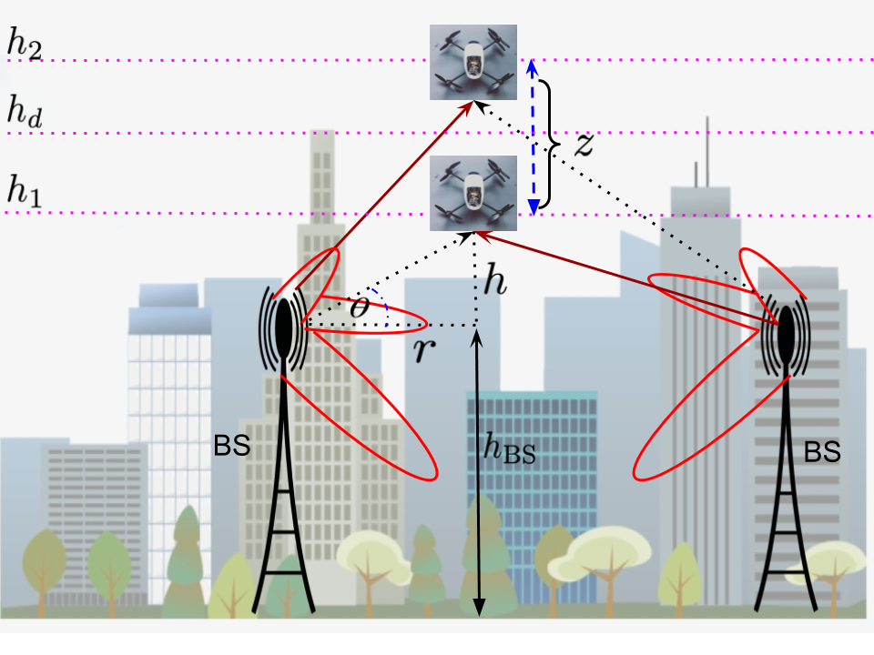
Figure 1: Illustration of the proposed system model in which 3D antenna-equipped ground BSs serve high-altitude static (or mobile) UAV-UEs.

II System Model

II-A Network Model

We consider a downlink transmission scenario from a terrestrial cellular network to cellular-connected UAV-UEs. We assume that ground BSs are distributed according to a two-dimensional (2D) homogeneous Poisson point process (PPP) $\Phi_{b}=\{b_{i}\in\mathbb{R}^{2},\forall i\in\mathbb{N}\}$ with intensity $\lambda_{b}$. All BSs have the same transmit power $P_{t}$ and are deployed at the same height $h_{\rm BS}$. We consider a number of UAV-UEs that can be either static or mobile based on the application. Static UAV-UEs hover at a fixed altitude $h_{d}$, while mobile ones can make up and down movements within two altitude thresholds $h_{1}$, and $h_{2}$. We set $h_{d}=\frac{h_{1}+h_{2}}{2}$, i.e., $h_{d}$ is the mean flying altitude of mobile UAV-UEs. As shown in Fig. 1, we consider high-altitude UAV-UEs where $h_{1}$, $h_{d}$, and $h_{2}$ are above the BS height $h_{\rm BS}$. Each UAV-UE has a single antenna and receives downlink signals from a ground BS. Each ground BS is equipped with a directional antenna array composed of $N_{t}$ vertically-placed elements. Two association schemes are considered for the UAV-UEs: Nearest and highest average received power (HARP) associations.

II-B Channel Model

We consider a wireless channel that is characterized by both small-scale and large-scale fading. For the large-scale fading, the channel between a ground BS and an UAV-UE is described by the LoS and non-line-of-sight (NLoS) components, which are considered separately along with their probabilities of occurrence [5]. This assumption is apropos for such ground-to-air channels that often exhibit LoS communication [5] and [12]. For small-scale fading, we adopt a Nakagami-$m_{v}$ model as done in [5] for the channel gain, whose probability distribution function (PDF) is given by: $f(\omega)=\frac{2m_{v}^{m_{v}}\omega^{2m_{v}-1}}{\Gamma(m_{v})}e^{-m_{v}\omega^{2}}$. The fading parameter $m_{v}$ is assumed to be an integer for tractability, where $v\in\{l,n\}$ accounts for LoS and NLoS communications, respectively. Given that $\omega\sim$ Nakagami$(m_{v})$, it directly follows that the channel gain power $\chi=\omega^{2}\sim\Gamma(m_{v},1/m_{v})$, which represents a Gamma random variable (RV) whose shape and scale parameters are $m_{v}$ and $\frac{1}{m_{v}}$, respectively. Hence, the PDF of channel power gain distribution will be: $f(\chi)=\frac{m_{v}^{m_{v}}\chi^{m-1}}{\Gamma(m_{v})}{\rm exp}\big{(}-m_{v}\chi\big{)}$.

3D blockage is characterized by the mean number of $\eta$ buildings/$\text{\,}\mathrm{k}\mathrm{m}$², the proportion $a$ of the total land area occupied by buildings, and the height of buildings modeled by a Rayleigh PDF with a scale parameter $c$. The probability of having a LoS communication from a BS at horizontal-distance $r$ from an UAV-UE is hence given, similar to [11] and [12], as

$$\mathbb{P}_{l}(r)=\prod_{n=0}^{{\rm max}(0,o-1)}\Bigg{[}1-{\rm exp}\Big{(}-\frac{\big{(}h_{\rm BS}+\frac{h(n+0.5)}{o}\big{)}^{2}}{2c^{2}}\Big{)}\Bigg{]},$$ (1)

where $h$ is the difference between the UAV-UE altitude and BS height and $o=\lfloor r\sqrt{a\eta}\rfloor$.

II-C Antenna Model

The ground BSs are equipped with directional antennas of fixed radiation patterns and with a down-tilt angle $\varphi$. This is typically achieved by equipping the BS with a uniform linear array (ULA) of $N_{t}$ vertically-placed elements, that are assumed to be omni-directional along the horizontal dimension [17]. Along the vertical dimension, the power radiation pattern is equal to the array factor times the radiation pattern of a single antenna. The $N_{t}$ antenna elements are equally spaced with adjacent elements separated by half of the wavelength. With the down-tilt angle $\varphi$, the overall array gain in the direction $\theta$ is given by [14]:

$$G(\theta)=\underbrace{\frac{1}{N_{t}}\frac{{\rm sin}^{2}\frac{N_{t}\pi}{2}\big{(}{\rm sin}(\theta)-{\rm sin}(\varphi)\big{)}}{{\rm sin}^{2}\frac{\pi}{2}\big{(}{\rm sin}(\theta)-{\rm sin}(\varphi)\big{)}}}_{A_{f}(\theta)}\times\underbrace{10^{{\rm min}(-1.2(\frac{\theta}{\delta})^{2},\frac{G_{m}}{10})}}_{G_{e}(\theta)},$$

where $G_{m}$ gives the threshold for antenna nulls, $A_{f}(\theta)$ is the array factor of the ULA, $G_{e}(\theta)$ is the element power gain of each antenna along the vertical dimension, i.e., the elevation angle $\theta$, and $\delta$ is the half power beamwidth. For simplicity, we assume that the gain $G_{e}(\theta)$ is a positive constant on the range of the elevation angle $\theta\in[0,\frac{\pi}{2}]$, and 0 otherwise (i.e., zero front-to-back power ratio as in [18]). From Fig. 1, $\theta={\rm arctan}(\frac{h}{r})$, where $r$ is a realization of the RV $R$ which represents the horizontal distance between a ground BS and the projection of an UAV-UE. If $G_{e}(\theta)$ is set to one, and for a zero down-tilt angle, the antenna array gain is simplified to:

$$G(r,h) =\frac{1}{N_{t}}\frac{{\rm sin}^{2}\frac{N_{t}\pi}{2}\big{(}{\rm sin}({\rm arctan}(\frac{h}{r}))\big{)}}{{\rm sin}^{2}\frac{\pi}{2}\big{(}{\rm sin}({\rm arctan}(\frac{h}{r}))\big{)}}.$$ (2)

Hence, the antenna gain plus path loss for the LoS and NLoS components will be: $\zeta_{v}(r)=A_{v}G(r,h)\big{(}r^{2}+h^{2}\big{)}^{-\alpha_{v}/2}$, where $v\in\{l,n\}$, $\alpha_{l}$ and $\alpha_{n}$ are the path loss exponents, and $A_{l}$ and $A_{n}$ are the path loss constants at $\sqrt{r^{2}+h^{2}}=$1\text{\,}\mathrm{m}$$ for the LoS and NLoS, respectively.

Having defined our system model, next, we will study the performance of UAV-UEs for two scenarios: static and mobile UAV-UEs. For each scenario, we investigate the UAV-UE coverage probability under two association schemes, namely, nearest and HARP associations. The coverage probability is defined as the probability that the received SIR is higher than a target threshold $\vartheta$.

III Coverage Probability of Static UAV-UEs

We assume static UAV-UEs hovering at a fixed altitude $h_{d}$, hence, we have $h=h_{d}-h_{\rm BS}$ in (1). Given that a PPP is translation invariant with respect to the origin, we conduct the coverage analysis for a UAV-UE located at the origin in $\operatorname*{\mathbb{R}}^{2}$, called the typical UAV-UE [19].

III-A Nearest Association

To simplify the analysis, we only consider probabilistic LoS/NLoS links for interfering BSs, while the serving BS has a dominant LoS component. This is because, at high altitude, UAV-UEs will have an LoS-dominated channel toward nearby, serving BSs. However, UAV-UE interference at far-away BSs will not be LoS dominated. Moreover, the study of LoS-based association is considered in prior works, e.g., [12], while we are particularly focused on the impact of practical antennas.

We denote the horizontal distance from the typical UAV-UE to its ground BS by $r_{0}$. By the PPP assumption, $f_{R_{0}}(r_{0})=2\pi r_{0}\lambda e^{-\pi\lambda r_{0}^{2}}$. Conditioning on $R_{0}=r_{0}$, and neglecting the noise, the received $\mathrm{SIR}$ at the typical UAV-UE will be:

$$\Upsilon_{|r_{0}} =\frac{\chi_{0}\zeta_{l}(r_{0})}{I},$$ (3)

where $I$ is the aggregate interference, $\chi_{0}$ is the Nakagami-$m_{l}$ fading power, and $\zeta_{l}(r_{0})$ represents the antenna gain plus path loss from the serving BS. The serving and interfering signals in (3) are normalized to the transmit power $P_{t}$. The UAV-UE coverage probability is characterized in the next Theorem.

Theorem 1.

The static UAV-UE coverage probability under nearest association is given by:

$$\mathbb{P}_{c}=\int_{r_{0}=0}^{\infty}\mathbb{P}_{c|r_{0}}f_{R_{0}}(r_{0})\differential{r_{0}},$$ (4)

where $\mathbb{P}_{c|r_{0}}$ is the UAV-UE conditional coverage probability:

$$\mathbb{P}_{c|r_{0}} \overset{}{=}\sum_{i=0}^{m_{l}-1}\frac{(-\varpi_{l})^{i}}{i!}\sum_{i_{n}+i_{l}=i}\frac{i!}{i_{n}!i_{l}!}\frac{\varpi_{l}^{i_{n}}}{i_{n}!}\frac{\partial^{i_{n}}}{\partial\varpi_{l}^{i_{n}}}\mathcal{L}_{I_{n}}(\varpi_{l})$$

$$\quad\quad\quad\quad\quad\quad\quad\quad\quad\quad\quad\times\frac{\varpi_{l}^{i_{l}}}{i_{l}!}\frac{\partial^{i_{l}}}{\partial\varpi_{l}^{i_{l}}}\mathcal{L}_{I_{l}}(\varpi_{l}),$$ (5)

and $\varpi_{l}=\frac{\vartheta d_{0}^{\alpha_{l}}m_{l}}{A_{l}G(r_{0},h)}$, $d_{0}=\sqrt{h^{2}+r_{0}^{2}}$; $\mathcal{L}_{I_{l}}$ and $\mathcal{L}_{I_{n}}$ are the Laplace transforms of the LoS and NLoS interference, respectively. The Laplace transform of LoS interference is then given by $\mathcal{L}_{I_{l}}(\varpi_{l})=e^{-\gamma(\varpi_{l})}$, where $\gamma(\varpi_{l})=2\pi\lambda_{b}\times$

$$\sum_{j=\lfloor r_{0}\sqrt{a\eta}\rfloor}^{\infty}\mathbb{P}_{l}(\frac{j}{\sqrt{a\eta}})\int_{{\rm max}(r_{0},\frac{j}{\sqrt{a\eta}})}^{\frac{j+1}{\sqrt{a\eta}}}\Big{(}1-\big{(}\frac{m_{l}}{m_{l}+\varpi_{l}\zeta_{l}(r)}\big{)}^{m_{l}}\Big{)}r\differential{r},$$

and the Laplace transform of NLoS interference is calculated following in the same manner.

Proof.

The sketch of the proof is found in the Appendix. ∎

Since it is hard to directly obtain insights from (4) on the effect of the practical antenna gain, several results based on (4) will be shown in Section V to provide key design guidelines. Moreover, we show that the coverage probability does not scale with $N_{t}$, which implies that increasing the number of antenna elements has a marginal effect on the coverage probability.

Corollary 1.

The coverage probability of static UAV-UEs does not scale asymptotically with the number of antenna elements.

Proof.

To study scalability, we consider a simple case with $m_{v}=A_{v}=1$, $v\in\{l,n\}$, hence, $\varpi_{l}=\frac{\vartheta d_{0}^{\alpha_{l}}}{G(r_{0},h)}$. We also assume that $N_{t}$ is small and $\frac{h}{r}\to 0$, which is a reasonable assumption for sparsely-deployed networks. The conditional coverage probability $\mathbb{P}_{c|r_{0}}$ is then simplified to:

$$\mathbb{P}_{c|r_{0}}=e^{-2\pi\lambda_{b}\int_{r=r_{0}}^{\infty}\frac{\varpi_{l}\zeta_{v}(r)r}{1+\varpi_{l}\zeta_{v}(r)}\differential{r}}$$

$$\overset{(a)}{\geq}1-2\pi\lambda_{b}\int_{r_{0}}^{\infty}\frac{\frac{\vartheta d_{0}^{\alpha_{l}}G(r,h)d^{-\alpha_{v}}}{G(r_{0},h)}}{1+\frac{\vartheta d_{0}^{\alpha_{l}}G(r,h)d^{-\alpha_{v}}}{G(r_{0},h)}}r\differential{r}$$

$$\overset{}{=}1-2\pi\lambda_{b}\int_{r_{0}}^{\infty}\frac{\vartheta d_{0}^{\alpha_{l}}G(r,h)d^{-\alpha_{v}}}{G(r_{0},h)+\vartheta d_{0}^{\alpha_{l}}G(r,h)d^{-\alpha_{v}}}r\differential{r},$$ (6)

where (a) follows from $e^{-x}\geq 1-x$. Recall that $G(r,h)=\frac{1}{N_{t}}\frac{{\rm sin}^{2}\frac{N_{t}\pi}{2}({\rm sin}({\rm arctan}(\frac{h}{r})))}{{\rm sin}^{2}\frac{\pi}{2}({\rm sin}({\rm arctan}(\frac{h}{r})))}$. From [20], we have ${\rm arctan}(\frac{h}{r})\simeq\frac{4h}{\pi r}$ and ${\rm sin}(\frac{4h}{\pi r})\simeq\frac{4h}{\pi r}$ for $h\ll r$, since ${\rm sin}(x)\simeq x$ for small $x$. Also, ${\rm sin}^{2}\frac{N_{t}\pi}{2}(\frac{4h}{\pi r})\simeq(\frac{2N_{t}h}{r})^{2}$ for small $N_{t}$ and $h\ll r$.

$$\mathbb{P}_{c|r_{0}} \overset{}{\simeq}1-2\pi\lambda_{b}\int_{r_{0}}^{\infty}\frac{\vartheta(d_{0}^{\alpha_{l}}/d^{\alpha_{v}})N_{t}}{N_{t}+\vartheta(d_{0}^{\alpha_{l}}/d^{\alpha_{v}})N_{t}}r\differential{r}$$

$$\overset{}{=}1-2\pi\lambda_{b}\int_{r_{0}}^{\infty}\frac{\vartheta(d_{0}^{\alpha_{l}}/d^{\alpha_{v}})}{1+\vartheta(d_{0}^{\alpha_{l}}/d^{\alpha_{v}})}r\differential{r}.$$ (7)

Since $\mathbb{P}_{c|r_{0}}$ in (III-A) is not a function of $N_{t}$, the UAV-UE coverage probability does not scale asymptotically with $N_{t}$, and the effect of $N_{t}$ on the coverage probability is minor. ∎

III-B Highest Average Received Power Association

Each UAV-UE is associated to the BS that delivers the highest average power, i.e., the effect of small scale fading is averaged. Hence, the received signal power depends on the path loss $d^{-\alpha_{v}}$ and antenna gain $G(r,h)$, which is, in turn, determined by the elevation angle $\theta$. In Fig. 2, we plot the path loss, antenna gain, and the overall link gain, i.e., the path loss times antenna gain, versus the horizontal distance $r$. From (2), the antenna gain consists of $\frac{N_{t}}{2}$ lobes whose peaks increase with the horizontal distance $r$. Fig. 2 also shows that the overall link gain (dashed line) consists of $\frac{N_{t}}{2}$ lobes whose maximum gains decrease as $r$ increases.

It is worth highlighting that obtaining the serving distance PDF is not possible given the non-convexity of the locations of BSs that deliver the highest power along $r$ (see Fig. 2). We hence propose a novel geometry-based approximation that leverages the relative symmetrical characteristics of the overall link gain. The key idea behind this approximation is to reproduce an equivalent PPP deployment of the BS locations in which the distance PDF to the BS delivering the highest average power (within each lobe) can be obtained. With this in mind, we can then obtain an expression approximating the UAV-UE coverage probability under HARP association. We particularly divide the space $r>0$ into $\frac{N_{t}}{2}$ regions, each of which corresponds to the boundary of one lobe. Then, for each lobe, we consider the zone from its peak to the next null, assuming doubled density of BSs. For instance, in Fig. 2, BSs of density $\lambda=2\lambda_{b}$ only exists within $r_{pj}$ to $r_{nj}$, $j\in\{1,\dots,\frac{N_{t}}{2}\}$. UAV-UEs then associate to the nearest BS from the reproduced deployment, which delivers the highest average power within its lobe. However, since this BS might not be the one that delivers the highest average power among all the BSs, the adopted method is an approximation.

From (2), there are $\frac{N_{t}}{2}$ nulls between the lobes that occur at elevation angles $\theta_{nj}$, where $\frac{N\pi}{2}{\rm sin}(\theta_{nj})=j\pi$. Hence, $\theta_{nj}={\rm arcsin}(\frac{2j}{N})$ and the equivalent horizontal distances at these nulls will be $r_{nj}=h/{\rm tan}\big{(}{\rm arcsin}(\frac{2j}{N})\big{)}$. For instance, $\theta_{n0}=0^{\circ}$ and $r_{n4}=\frac{h}{{\rm tan}(0)}=\infty$ (where the indices are reversed for the distance). To obtain the locations of peaks $r_{pj}$, we define the overall link gain as $L(\theta)=G(\theta)\times d^{-\alpha_{v}}$:

$$L(\theta)=\frac{1}{N_{t}}\frac{{\rm sin}^{2}\frac{N_{t}\pi}{2}\big{(}{\rm sin}(\theta)\big{)}}{{\rm sin}^{2}\frac{\pi}{2}\big{(}{\rm sin}(\theta)\big{)}}\times\big{(}r^{2}+h^{2}\big{)}^{-\alpha_{v}/2}$$

$$\overset{(a)}{=}\frac{1}{N_{t}h^{\alpha_{v}}}\frac{{\rm sin}^{2}\frac{N_{t}\pi}{2}\big{(}{\rm sin}(\theta)\big{)}}{{\rm sin}^{2}\frac{\pi}{2}\big{(}{\rm sin}(\theta)\big{)}\big{(}{\rm tan}^{-2}(\theta)+1\big{)}^{\alpha_{v}/2}},$$

where (a) follows from ${\rm tan}(\theta)=\frac{h}{r}$. We find elevation angles $\theta_{pj}$ at which the peaks occur by taking the first derivative of $L(\theta)$ and set it to zero. The first derivative is obtained as:

$$\frac{\partial L(\theta)}{\partial\theta} =(N_{t}-1){\rm sin}(\frac{\pi(N_{t}+1)}{2}{\rm sin}(\theta))+$$

$$(N_{t}+1){\rm sin}(\frac{\pi(1-N_{t})}{2}{\rm sin}(\theta))+$$

$$\frac{\alpha_{v}\big{(}{\rm cos}(\frac{\pi(N_{t}-1)}{2}{\rm sin}(\theta))-{\rm cos}(\frac{\pi(N_{t}+1)}{2}{\rm sin}(\theta)\big{)}}{\pi{\rm cos}(\theta){\rm tan}(\theta)\big{(}1+{\rm tan}^{2}(\theta)\big{)}}=0.$$

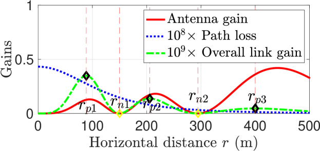
Figure 2: Illustration of the geometry-based approximation to calculate the UAV-UE coverage probability under HARP association.

The roots of this equation are $\theta_{pj}$, and equivalent distances are $r_{pj}=\frac{h}{{\rm tan}(\theta_{pj})}$. The density of BSs within [$r_{jp},r_{jn}]$ is $\lambda=2\lambda_{b}$, and zero otherwise. From the PPP definition, the probability that at least one BS exists within $[r_{pj},r_{nj}]$ in the reproduced deployment is $1-e^{-\pi\lambda(r_{nj}^{2}-r_{pj}^{2})}$. Hence, the piece-wise serving distance cumulative distribution function (CDF) will be $F_{R_{m}}(r_{m})=$

$$\left\{\begin{array}[]{ll}\Big{(}1-e^{-\pi\lambda(r_{m}^{2}-r_{p1}^{2})}\Big{)}\Big{(}1-e^{-\pi\lambda(r_{n1}^{2}-r_{p1}^{2})}\Big{)},\quad\quad j=1\\ \Big{(}1-e^{-\pi\lambda(r_{m}^{2}-r_{pj}^{2})}\Big{)}\Big{(}1-e^{-\pi\lambda(r_{nj}^{2}-r_{pj}^{2})}\Big{)}\times\\ \prod_{i=1}^{j-1}e^{-\pi\lambda(r_{ni}^{2}-r_{pi}^{2})},\quad\quad\quad\quad\quad\quad\quad\quad\quad 1<j\leq\frac{N_{t}}{2}\\ 0,\quad\quad\quad\quad\quad\quad\quad\quad\quad\quad\quad\quad\quad\quad\quad\quad\quad{\rm otherwise}\end{array}\right.$$

where the product term represents the probability that no BSs exist in the previous lobes. Hence, the serving distance PDF will be $f_{R_{m}}(r_{m})=\frac{\partial F_{R_{m}}(r_{m})}{\partial r_{m}}=$

$$\left\{\begin{array}[]{ll}2\pi\lambda r_{m}e^{-\pi\lambda(r_{m}^{2}-r_{p1}^{2})}\Big{(}1-e^{-\pi\lambda(r_{n1}^{2}-r_{p1}^{2})}\Big{)},\quad\quad j=1\\ 2\pi\lambda r_{m}e^{-\pi\lambda(r_{m}^{2}-r_{pj}^{2})}\Big{(}1-e^{-\pi\lambda(r_{nj}^{2}-r_{pj}^{2})}\Big{)}\times\\ \prod_{i=1}^{j-1}e^{-\pi\lambda(r_{ni}^{2}-r_{pi}^{2})},\quad\quad\quad\quad\quad\quad\quad\quad\quad 1<j\leq\frac{N_{t}}{2}\\ 0,\quad\quad\quad\quad\quad\quad\quad\quad\quad\quad\quad\quad\quad\quad\quad\quad\quad{\rm otherwise.}\end{array}\right.$$

It can be easily verified that $\int_{r_{m}=0}^{\infty}f_{R_{m}}(r_{m})=1$. Given $f_{R_{m}}(r_{m})$, the approximated coverage probability under HARP association is characterized in the next corollary.

Corollary 2.

The coverage probability of static UAV-UEs under HARP association is approximated as:

$$\mathbb{P}_{c}=\int_{r_{m}=0}^{\infty}\mathbb{P}_{c|r_{m}}f_{R_{m}}(r_{m})\differential{r_{m}},$$ (8)

where $\mathbb{P}_{c|r_{m}}$ is calculated similar to $\mathbb{P}_{c|r_{0}}$ in Theorem 1, with $\varpi_{l}=\frac{\vartheta d_{m}^{\alpha_{l}}m_{l}}{A_{l}G(r_{m},h)}$, $d_{m}=\sqrt{h^{2}+r_{m}^{2}}$, and $\gamma(\varpi_{l})=2\pi\lambda_{b}\times\sum_{j=0}^{\infty}\mathbb{P}_{l}(\frac{j}{\sqrt{a\eta}})\int_{\frac{j}{\sqrt{a\eta}}}^{\frac{j+1}{\sqrt{a\eta}}}\Big{(}1-\big{(}\frac{m_{l}}{m_{l}+\varpi_{l}\zeta_{l}(r)}\big{)}^{m_{l}}\Big{)}r\differential{r}$.

The proof of Corollary 2 follows from Theorem 1. As discussed previously, the cell association of UAV-UEs and their overall performance is essentially driven by the availability of LoS links and the encountered antenna gain. Thus far, we particularly showed that the coverage probability of static UAV-UEs heavily depends on the antenna pattern, but it does not scale with the number of antenna elements. Next, we study a scenario in which the UAV-UEs can be mobile.

IV Coverage Probability of mobile UAV-UEs

We consider vertically-mobile UAV-UEs that make frequent up and down movements with a fixed velocity $\bar{\nu}$ in the finite vertical region $[h_{1},h_{2}]$. We refer to it as vertical 1D random waypoint (RWP) mobility model. Similar stochastic mobility models are adopted for UAV-BSs and UAV-UEs in the recent works [10] and [21, 22, 23, 24]. The proposed mobility model works as follows: Initially, at time instant $t_{0}$, the UAV-UE is at an arbitrary altitude $h_{0}$ selected uniformly from the interval $[h_{1},h_{2}]$. Then, at next time epoch $t_{1}$, this UAV-UE at $h_{0}$ selects a new random waypoint $h_{1}$ uniformly in $[h_{1},h_{2}]$, and moves towards it. Once the UAV-UE reaches $h_{1}$, it repeats the same procedure to find the next destination altitude and so on. Eventually, the steady-state altitude distribution converges to a non-uniform distribution $F_{Z}(z)$. Note that random waypoints refer to the altitude of a UAV-UE at each time epoch, which is uniformly-distributed in $[h_{1},h_{2}]$, while vertical transitions are the differences in the UAV-UE altitude throughout its trajectory. While the random waypoints are independent and uniformly-distributed by definition, the random lengths of vertical transitions are statistically dependent. This is because the endpoint of one movement epoch is the starting point of the next epoch. In [10], we showed that $f_{Z}(z)=\frac{h_{1}z+h_{2}z-h_{1}h_{2}-z^{2}}{\hbar^{3}/6}$, $\forall h_{1}<z<h_{2}$, where $\hbar=h_{2}-h_{1}$. It can be easily verified that the mean altitude is $\mathbb{E}[Z]=\frac{h_{1}+h_{2}}{2}$.

The coverage mobility of UAV-UEs is studied under nearest and HARP associations. Vertically-mobile UAV-UEs under nearest association maintain their connection to the nearest BSs. However, since UAV-UEs under HARP association connect to the BS delivering the highest average power, the serving BS might change with the UAV-UE altitude. This is because the elevation angle and, correspondingly, the BS antenna gain change with the UAV-UE altitude.

IV-A Nearest Association

For vertically mobile UAV-UEs, the distance to the nearest BS is denoted as $w_{0}=\sqrt{r_{0}^{2}+(z-h_{\rm BS})^{2}}$, with $w_{0}\geq h_{0}$, and $h_{0}=h_{1}-h_{\rm BS}$. For simplicity, we use $f_{Z}(z)$ to obtain the steady state 3D distance PDF $f_{W_{0}}(w_{0})$, rather than averaging over two RVs $Z$ and $R_{0}$ in the coverage probability calculation. Since $R_{0}$ and $Z$ are two independent RVs, $f_{R_{0},Z}(r_{0},z)=f_{R_{0}}(r_{0})f_{Z}(z)$. Given that, we transform the two RVs $R_{0}$ and $Z$ to $W_{0}$ and find $f_{W_{0}}(w_{0})$, with the details omitted due to the limited space. The equivalent 3D distance PDF is obtained as $f_{W_{0}}(w_{0})=2\pi\lambda_{b}w_{0}\Omega(h_{1},h_{2})e^{-\pi\lambda_{b}w_{0}^{2}}$, where $\Omega(h_{1},h_{2})=\frac{\psi(h_{2})(1-\varkappa)-\psi(h_{1})(\varkappa+1)+2\kappa(h_{1},h_{2})-2\kappa(h_{2},h_{1})}{2\pi\lambda_{b}^{3/2}\hbar^{3}/3}$, $\psi(x)=\text{erfi}\left(\sqrt{\pi}\sqrt{\lambda_{b}}(x-h_{\rm BS})\right)$, $\varkappa=2\pi\lambda_{b}(h_{1}-h_{\rm BS})(h_{\rm BS}-h_{2})$, and $\kappa(x,y)=\sqrt{\lambda_{b}}(x-h_{\rm BS})e^{\pi\lambda_{b}(y-h_{\rm BS})^{2}}$.

Since $w_{0}$ replaces both $z$ and $r_{0}$, we set $\theta$ to ${\rm arcsin}(\frac{h}{w_{0}})$ in (2) to obtain the antenna gain $G(w_{0},h)$, where $h=h_{d}-h_{\rm BS}$ and $h_{d}=\mathbb{E}[Z]=\frac{h_{1}+h_{2}}{2}$ is the mean flying altitude. The effect of the vertical mobility, i.e., altitude variation, and horizontal distance randomness are now captured by the RV $W_{0}$.

We characterize the coverage probability of mobile UAV-UEs under nearest association in the next corollary (whose proof follows Theorem 1).

Corollary 3.

The coverage probability of mobile UAV-UEs under nearest association is given by:

$$\mathbb{P}_{c}=\int_{h_{0}}^{\infty}\mathbb{P}_{c|w_{0}}f_{W_{0}}(w_{0})\differential{w_{0}},$$ (9)

where $\mathbb{P}_{c|w_{0}}$ is calculated as in (5), with $\varpi_{l}=\frac{\vartheta w_{0}^{\alpha_{l}}m_{l}}{A_{l}G(w_{0},h)}$. The Laplace transform of LoS interference is given by $\mathcal{L}_{I_{l}}(\varpi_{l})=e^{-\gamma(\varpi_{l})}$, where $\gamma(\varpi_{l})=2\pi\lambda_{b}\sum_{j=j_{0}}^{\infty}\mathbb{P}_{l}(s)\int_{{\rm max}(w_{0},s)}^{t}\Big{(}1-\big{(}\frac{m_{l}}{m_{l}+\varpi_{l}A_{l}G(w,h)w^{-\alpha_{l}}}\big{)}^{m_{l}}\Big{)}w\differential{w}$, $j_{0}=\lfloor\sqrt{w_{0}^{2}-h^{2}}\sqrt{a\eta}\rfloor$, $s=\frac{j}{\sqrt{a\eta+h^{2}}}$, $t=\frac{j+1}{\sqrt{a\eta+h^{2}}}$, and $\mathbb{P}_{l}(j)$ is calculated from (1).

The antenna gain effect on the coverage probability of mobile UAV-UEs can be interpreted in a similar way to the static scenario in (1). Particularly, conditioning on $W_{0}=w_{0}$, the yielded expression holds the same insights as for static users, i.e., the coverage probability does not scale with $N_{t}$.

IV-B Highest Average Received Power Association

Mobile UAV-UEs under HARP association are prone to frequent altitude handovers. This happens when their trajectory crosses multiple peaks and nulls of the antennas’ side-lobes. For instance, Fig. 1 shows that the UAV-UE at altitude $h_{1}$ associates to the right BS, while it turns to attach to the left BS at altitude $h_{2}$. This altitude handover negatively impacts the performance of UAV-UEs as it results in dropped connections. In fact, the elevation angle $\theta=\arctan(\frac{z-h_{\rm BS}}{r_{m}})$ plays a crucial role on determining the serving BS. Hence, it essential to average over the random distance $R_{m}$ (as in Corollary 2) for every possible $Z$, to correctly account for the handover and cell selection. Motivated by this fact, we describe the coverage probability as stated in the next corollary.

Corollary 4.

The approximated coverage probability of mobile UAV-UEs under HARP association is described as:

$$\mathbb{P}_{c}=\int_{z=h_{1}}^{h_{2}}\int_{r_{m}=0}^{\infty}\mathbb{P}_{c|r_{m},z}f_{R_{m}}(r_{m})f_{Z}(z)\differential{r_{m}}\differential{z},$$ (10)

where $\mathbb{P}_{c|r_{m},z}$ is calculated as $\mathbb{P}_{c|r_{0}}$ in Theorem 1, with $\varpi_{l}=\frac{\vartheta(r_{m}^{2}+(z-h_{\rm BS}))^{\alpha_{l}/2}m_{l}}{A_{l}G(r_{m},z-h_{\rm BS})}$. The Laplace transform of LoS interference is $\mathcal{L}_{I_{l}}(\varpi_{l})=e^{-\gamma(\varpi_{l})}$, where $\gamma(\varpi_{l})=2\pi\lambda_{b}\sum_{j=0}^{\infty}\mathbb{P}_{l}(j)\int_{\frac{j}{\sqrt{a\eta}}}^{\frac{j+1}{\sqrt{a\eta}}}\Big{(}1-\big{(}\frac{m_{l}}{m_{l}+\varpi_{l}\zeta_{l}(r)}\big{)}^{m_{l}}\Big{)}r\differential{r}$.

To account for the UAV-UE mobility in the coverage probability expression, similar to [10] and [11], we consider a linear function that reflects the cost of handovers. Particularly, we define the mobile UAV-UE coverage probability as:

$$\mathbb{P}_{c}(\bar{\nu},\lambda_{b},\beta)=(1-\beta)\mathbb{P}_{c}+\beta\mathbb{P}(\bar{H})\mathbb{P}_{c},$$ (11)

where $\beta\in[0,1]$ represents the handover cost and $\mathbb{P}(\bar{H})$ is the probability of no handover. The handover probability is defined as the probability that an UAV-UE associates to a new BS rather than the serving BS after a unit time. It is clear from (11) that, if $\beta=1$, the first term vanishes and the UAV-UE will be in coverage only if there is no handover associated with its mobility.

V Numerical Results

For our simulations, we consider a network having the parameter values indicated in Table I.

TABLE I: Simulation Parameters

Description	Parameter	Value
LoS and NLoS path-loss exponents	$\alpha_{l}$, $\alpha_{n}$	2.09, 3.75
LoS and NLoS path-loss constants	$A_{l}$, $A_{n}$	-41.1, $-32.9\text{\,}\mathrm{d}\mathrm{B}$
Number of antenna elements	$N_{t}$	8
LoS and NLoS fading parameters	$m_{l}$, $m_{n}$	3, 1
BS height and UAV-UE altitude	$h_{\textrm{BS}}$, $h_{d}$	$30\text{\,}\mathrm{m}$, $150\text{\,}\mathrm{m}$
UAV-UE lowest and highest altitudes	$h_{1}$, $h_{2}$	$140\text{\,}\mathrm{m}$, $160\text{\,}\mathrm{m}$
Mobile UAV-UE speed	$\bar{\nu}$	$20\text{\,}\mathrm{k}\mathrm{m}\mathrm{h}$
Environment blocking parameters	$a$, $\eta$, $c$	0.6, $500\text{\,}\mathrm{k}\mathrm{m}$-2, $30\text{\,}\mathrm{m}$
Density of BSs and $\mathrm{SIR}$ threshold	$\lambda_{b}$, $\vartheta$	$50\text{\,}\mathrm{k}\mathrm{m}$-2, $-15\text{\,}\mathrm{dB}$

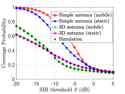
Figure 3: Coverage probability of static and mobile UAV-UEs under nearest association scheme versus the SIR threshold $\vartheta$.

V-A Nearest Association

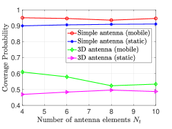
Figure 4: Coverage probability of static and mobile UAV-UEs under nearest association versus the number of antenna elements $N_{t}$.

We first evaluate the performance of static and mobile UAV-UEs under the nearest association scheme. We compare the UAV-UE coverage probability under practical antenna patterns with that adopting simple antenna models, e.g., [11, 12, 10]. Particularly, high-altitude UAV-UEs are essentially served and interfered from the antennas’ side-lobes. Hence, for a simple antenna model, the antenna gain effect is normalized. Fig. 3 first shows that the performance attained under a simple antenna model is superior to that from a practical antenna pattern. This implies that adopting practical antenna models is vital to convey a realistic performance evaluation of the UAV-UEs. Fig. 3 also compares the performance of mobile UAV-UEs to static counterparts under nearest association. The effect of vertical mobility on the UAV-UE coverage probability is relatively marginal. This is attributed to the fact that there is no altitude handover associated with the vertical mobility as the UAV-UE maintains its connection with the nearest BS.

Fig. 4 investigates the prominent effect of the number antenna elements $N_{t}$ on the UAV-UE coverage probability. Fig. 4 shows that an increase in the number of antenna elements has an intangible effect on the coverage probability of static and mobile UAV-UEs under nearest association, hence verifying the claim in Corollary 1. This also can be interpreted by the fact that, while increasing $N_{t}$ yields a higher number of lobes, the integrands in the coverage probability expression, which are functions of the antenna gains, constitute an overall area that does not significantly change with $N_{t}$.

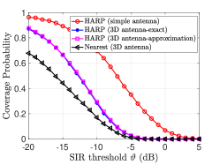
Figure 5: Coverage probability of static UAV-UEs under HARP association ($m_{v}=1$, $N_{t}=4$).

V-B HARP Association

Next, we discuss the performance of UAV-UEs under HARP association. Fig. 5 verifies the accuracy of the geometry-based approximation of Corollary 2. Fig. 5 presents the exact and the obtained approximation of the static UAV-UE coverage probability versus the SIR threshold $\vartheta$. Clearly, the adopted approximation is relatively tight. Fig. 5 also shows that the coverage probability of static UAV-UEs under practical antenna patterns is much reduced compared to the achievable coverage probability from a simple antenna model.

In Fig. 6, we plot the coverage probability of mobile UAV-UEs versus the number of antenna elements $N_{t}$, at different penalty costs $\beta$. Fig. 6 shows that the UAV-UE coverage probability monotonically decreases as both $N_{t}$ and $\beta$ increase. This can be interpreted by the fact that as long as $N_{t}$ increases, the mobile UAV-UE becomes more susceptible to handovers, which are penalized by the cost $\beta$.

Finally, Fig. 7 investigates the relation between the handover rate $H$ ($\text{\,}\mathrm{s}\mathrm{e}\mathrm{c}^{-1}$) and the number of antenna elements $N_{t}$. The handover rate is numerically calculated from

$$H=\mathbb{E}\Big{[}\frac{\#\text{ handoffs per each movement}}{\text{movement length}}\Big{]}\times\bar{\nu},$$

where the movement is generated according to the adopted vertical mobility model. Fig. 7 shows that the handover rate monotonically grows with the number of antenna elements. This is due to the higher number of nulls and peaks of the antenna vertical gain the UAV-UE crosses along its trajectory. From this result, we conclude that a larger number of antenna elements yields a higher rate of altitude handovers.

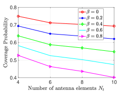
Figure 6: Coverage probability of mobile UAV-UEs under HARP association ($h_{d}=$100\text{\,}\mathrm{m}$$, $h_{1}=$80\text{\,}\mathrm{m}$$, $h_{2}=$120\text{\,}\mathrm{m}$$).

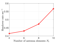
Figure 7: The handover rate versus the number of antenna elements ($h_{d}=$100\text{\,}\mathrm{m}$$, $h_{1}=$80\text{\,}\mathrm{m}$$, $h_{2}=$120\text{\,}\mathrm{m}$$).

VI Conclusion

In this paper, we have studied the performance of UAV-UEs under practical antenna configurations. The coverage probability of static and mobile UAV-UEs are characterized as functions of the system parameters, namely, the number of antenna elements, density of BSs, and the UAV-UE altitude for both nearest and HARP associations. The handover rate is also investigated to reveal the impact of practical antenna pattern on the cell association of mobile UAV-UEs. We have shown that the overall performance under practical antenna patterns is worse than that attained from a simple antenna model. Moreover, for static UAV-UEs, or mobile static UAV-UEs undergoing nearest association, the increase of the number of the antenna elements is shown to have a slight impact on their achievable performance. Conversely, for HARP association, the coverage probability of mobile UAV-UE decreases as the number of antenna elements increases due to the excessive rate of altitude handover that is penalized by the handover cost $\beta$.

We first let $d=\sqrt{h^{2}+r^{2}}$ denote the communication link distance. The conditional coverage probability is given by:

$$\mathbb{P}_{c|r_{0}}=\mathbb{P}\Big{(}\frac{\Upsilon_{|r_{0}}}{I}>\vartheta\Big{)}=\mathbb{P}\Big{(}\frac{\chi_{0}\zeta_{l}(r_{0})}{I}>\vartheta\Big{)}$$

$$=\mathbb{P}\Big{(}\chi_{0}>\frac{\vartheta d_{0}^{\alpha_{l}}}{A_{l}G(r_{0},h)}I\Big{)}\overset{(a)}{=}\sum_{i=0}^{m_{l}-1}\Big{(}\frac{\vartheta d_{0}^{\alpha_{l}}m_{l}}{A_{l}G(r_{0},h)}\Big{)}^{i}\frac{1}{i!}I^{i}\times$$

$$e^{-\frac{\vartheta d_{0}^{\alpha_{l}}m_{l}}{A_{l}G(r_{0},h)}I}\overset{(b)}{=}\Big{[}\sum_{i=0}^{m_{l}-1}\frac{(-\varpi_{l})^{i}}{i!}\frac{\partial^{i}}{\partial\varpi_{l}^{i}}\mathcal{L}_{I}(\varpi_{l})\Big{]},$$ (12)

where (a) follows from the PDF of the Gamma RV $\chi_{0}$, (b) follows from the Laplace transform of aggregate interference, i.e., the RV $I$. The LoS and NLoS interfering BSs are distributed independently of one another [12]. Let $\lambda_{v}^{\prime}(r)=2\pi\lambda_{b}r\mathbb{P}_{v}(r)$, $v\in\{l,n\}$, be the density of the inhomogeneous PPPs modeling each kind of the two interfering BS types. Hence, the Laplace transform of interference can be separated into a product of the Laplace transforms of the LoS and NLoS interference. Accordingly, the coverage probability will be [12]:

$$\mathbb{P}_{c|r_{0}} \overset{}{=}\sum_{i=0}^{m_{l}-1}\frac{(-\varpi_{l})^{i}}{i!}\sum_{i_{n}+i_{l}=i}\frac{i!}{i_{n}!i_{l}!}\frac{\varpi_{l}^{i_{n}}}{i_{n}!}\frac{\partial^{i_{n}}}{\partial\varpi_{l}^{i_{n}}}\mathcal{L}_{I_{n}}(\varpi_{l})$$

$$\quad\quad\quad\quad\quad\quad\quad\quad\quad\quad\quad\times\frac{\varpi_{l}^{i_{l}}}{i_{l}!}\frac{\partial^{i_{l}}}{\partial\varpi_{l}^{i_{l}}}\mathcal{L}_{I_{l}}(\varpi_{l}),$$ (13)

where $\mathcal{L}_{I_{l}}$ and $\mathcal{L}_{I_{n}}$ are the Laplace transforms of the LoS and NLoS interference, respectively. The second sum is over all of the combinations of non-negative integers $i_{l}$ and $i_{n}$. We obtain the Laplace transform of LoS interference $\mathcal{L}_{I_{l}}(\varpi_{l})$, whereas the NLoS interference follows in the same manner.

$$\mathcal{L}_{I_{l}}(\varpi_{l})=\mathbb{E}_{I_{l}}\Big{[}e^{-\varpi_{l}I_{l}}\Big{]}=\mathbb{E}\Bigg{[}e^{-\varpi_{l}\sum_{r\in\Phi_{b}^{!}}\chi_{r}\zeta_{l}(r)}\Bigg{]}$$

$$=\mathbb{E}_{\Phi_{b},\chi_{r}}\Bigg{[}\prod_{r\in\Phi_{b}^{!}}e^{-\varpi_{l}\chi_{r}\zeta_{l}(r)}\Bigg{]}=\mathbb{E}_{\Phi_{b}}\Bigg{[}\prod_{r\in\Phi_{b}^{!}}\mathbb{E}_{\chi_{r}}e^{-\varpi_{l}\chi_{r}\zeta_{l}(r)}\Bigg{]}$$

$$\overset{(a)}{=}\mathbb{E}_{\Phi_{b}}\Bigg{[}\prod_{r\in\Phi_{b}^{!}}\Big{(}\frac{m_{v}}{m_{v}+\varpi_{l}\zeta_{l}(r}\Big{)}^{m_{v}}\Bigg{]},$$ (14)

where $\Phi_{b}^{!}=\Phi_{b}\setminus r_{0}$ and (a) follows from $\chi_{r}\sim\Gamma(m_{v},\frac{1}{m_{v}})$. Using the probability generating functional (PGFL) of PPP and the density of LoS interferers $\lambda_{l}^{\prime}(r)=2\pi\lambda_{b}r\mathbb{P}_{l}(r)$, the Laplace transform of LoS interference will be $\mathcal{L}_{I_{l}}(\varpi_{l})=$

$$=e^{-\overbrace{2\pi\lambda_{b}\int_{r_{0}}^{\infty}\mathbb{P}_{l}(r)\Big{(}1-\big{(}\frac{m_{l}}{m_{l}+\varpi_{l}\zeta_{l}(r)}\big{)}^{m_{l}}\Big{)}r\differential{r}}^{\gamma(\varpi_{l})}}.$$ (15)

From (1), $\mathbb{P}_{l}(r)$ is a step function of the serving distance $r$. We use this fact to separate the integral above into a sum of weighted integrals, resulting in $\gamma(\varpi_{l})=2\pi\lambda_{b}\times$

$$\sum_{j=\lfloor r_{0}\sqrt{a\eta}\rfloor}^{\infty}\mathbb{P}_{l}(\varsigma)\int_{{\rm max}(r_{0},\frac{j}{\sqrt{a\eta}})}^{\frac{j+1}{\sqrt{a\eta}}}\Big{(}1-\big{(}\frac{m_{l}}{m_{l}+\varpi_{l}\zeta_{l}(r)}\big{)}^{m_{l}}\Big{)}r\differential{r}.$$

Substituting (15) into (13) yields the conditional coverage probability $\mathbb{P}_{c|r_{0}}$. Given the nearest distance PDF $f_{R_{0}}(r_{0})$, the unconditional coverage probability is obtained.

[25, 26, 27, 28, 29, 30, 31, 32, 33, 34, 35, 36, 37] [38, 39, 40, 41, 42, 43, 44, 45, 46] [47, 48, 49]

References

- [1] M. Mozaffari, W. Saad, M. Bennis, Y. Nam, and M. Debbah, “A tutorial on UAVs for wireless networks: Applications, challenges, and open problems,” IEEE Communications Surveys Tutorials, pp. 1–1, 2019.
- [2] M. Mozaffari, W. Saad, M. Bennis, and M. Debbah, “Unmanned aerial vehicle with underlaid device-to-device communications: Performance and tradeoffs,” IEEE Transactions on Wireless Communications, vol. 15, no. 6, pp. 3949–3963, June 2016.
- [3] W. Saad, M. Bennis, and M. Chen, “A vision of 6G wireless systems: Applications, trends, technologies, and open research problems,” IEEE Network, to appear, 2019.
- [4] M. A. Kishk, A. Bader, and M.-S. Alouini, “On the 3-d placement of airborne base stations using tethered uavs,” arXiv preprint arXiv:1907.04299, 2019.
- [5] M. M. Azari, F. Rosas, A. Chiumento, and S. Pollin, “Coexistence of terrestrial and aerial users in cellular networks,” in Proc. of IEEE Globecom Workshops (GC Wkshps), Singapore, Dec 2017, pp. 1–6.
- [6] X. Lin, V. Yajnanarayana, S. D. Muruganathan, S. Gao, H. Asplund, H.-L. Maattanen, M. Bergstrom, S. Euler, and Y.-P. E. Wang, “The sky is not the limit: LTE for unmanned aerial vehicles,” IEEE Communications Magazine, vol. 56, no. 4, pp. 204–210, April 2018.
- [7] S. Zhang, Y. Zeng, and R. Zhang, “Cellular-enabled UAV communication: A connectivity-constrained trajectory optimization perspective,” IEEE Transactions on Communications, vol. 67, no. 3, 2019.
- [8] R. Amer, W. Saad, H. ElSawy, M. Butt, and N. Marchetti, “Caching to the sky: Performance analysis of cache-assisted CoMP for cellular-connected UAVs,” in Proc. of the IEEE Wireless Communications and Networking Conference (WCNC), Marrakech, Morocco, April. 2019.
- [9] R. Amer, W. Saad, and N. Marchetti, “Towards a connected sky: Performance of beamforming with down-tilted antennas for ground and UAV user co-existence,” IEEE Communications Letters, pp. 1–1, 2019.
- [10] R. Amer, W. Saad, and N. Marchetti, “Mobility in the sky: Performance and mobility analysis for cellular-connected UAVs,” arXiv preprint arXiv:1908.07774, 2019.
- [11] M. M. Azari, F. Rosas, and S. Pollin, “Cellular connectivity for UAVs: Network modeling, performance analysis and design guidelines,” IEEE Transactions on Wireless Communications, pp. 1–1, 2019.
- [12] B. Galkin, J. Kibilda, and L. Da Silva, “A stochastic model for UAV networks positioned above demand hotspots in urban environments,” IEEE Transactions on Vehicular Technology, pp. 1–1, 2019.
- [13] G. Geraci, A. Garcia-Rodriguez, L. G. Giordano, D. López-Pérez, and E. Björnson, “Understanding UAV cellular communications: From existing networks to massive MIMO,” IEEE Access, vol. 6, 2018.
- [14] X. Xu and Y. Zeng, “Cellular-connected UAV: Performance analysis with 3D antenna modelling,” in IEEE International Conference on Communications Workshops (ICC Workshops), May 2019, pp. 1–6.
- [15] S. Euler, H. Maattanen, X. Lin, Z. Zou, M. Bergström, and J. Sedin, “Mobility support for cellular connected unmanned aerial vehicles: Performance and analysis,” 2018. [Online]. Available: http://arxiv.org/abs/1804.04523
- [16] A. Fakhreddine, C. Bettstetter, S. Hayat, R. Muzaffar, and D. Emini, “Handover challenges for cellular-connected drones,” in Proc. of ACM Workshop on Micro Aerial Vehicle Networks, Systems, and Applications, NY, USA, 2019, pp. 9–14.
- [17] G. T. 36.777, “Technical specification group radio access network; study on enhanced LTE support for aerial vehicles,” tech. rep., 5G Americas, Dec. 2017.
- [18] T.-T. Vu, L. Decreusefond, and P. Martins, “An analytical model for evaluating outage and handover probability of cellular wireless networks,” Wireless personal communications, vol. 74, no. 4, pp. 1117–1127, 2014.
- [19] M. Haenggi, Stochastic geometry for wireless networks. Cambridge University Press, 2012.
- [20] S. Rajan, S. Wang, R. Inkol, and A. Joyal, “Efficient approximations for the arctangent function,” IEEE Signal Processing Magazine, vol. 23, no. 3, pp. 108–111, 2006.
- [21] P. K. Sharma and D. I. Kim, “Random 3D mobile UAV networks: Mobility modeling and coverage probability,” IEEE Transactions on Wireless Communications, vol. 18, no. 5, pp. 2527–2538, May 2019.
- [22] M. Banagar and H. S. Dhillon, “Performance characterization of canonical mobility models in drone cellular networks,” arXiv preprint arXiv:1908.05243, 2019.
- [23] ——, “Fundamentals of drone cellular network analysis under random waypoint mobility model,” in Proc. of the IEEE Global Communication Conference (Globecom), Hawaii, USA, Dec. 2019.
- [24] ——, “3GPP-inspired stochastic geometry-based mobility model for a drone cellular network,” in Proc. of the IEEE Global Communication Conference (Globecom), Hawaii, USA, Dec. 2019.
- [25] M. Baza, N. Lasla, M. Mahmoud, G. Srivastava, and M. Abdallah, “B-ride: Ride sharing with privacy-preservation, trust and fair payment atop public blockchain,” arXiv preprint arXiv:1906.09968, 2019.
- [26] M. Baza, M. Mahmoud, G. Srivastava, W. Alasmary, and M. Younis, “A light blockchain-powered privacy-preserving organization scheme for ride sharing services,” Proc. of the IEEE 91th Vehicular Technology Conference (VTC-Spring), Antwerp, Belgium, May 2020.
- [27] M. Baza, A. Salazar, M. Mahmoud, M. Abdallah, and K. Akkaya, “On sharing models instead of the data for smart health applications,” Proc. of IEEE International Conference on Informatics, IoT, and Enabling Technologies (ICIoT’20), Doha, Qatar, 2020.
- [28] W. Al Amiri, M. Baza, M. Mahmoud, W. Alasmary, and K. Akkaya, “Towards secure smart parking system using blockchain technology,” Proc. of 17th IEEE Annual Consumer Communications Networking Conference (CCNC), Las vegas, USA, 2020.
- [29] ——, “Privacy-preserving smart parking system using blockchain and private information retrieval,” Proc. of the IEEE SmartNets, 2020.
- [30] M. Baza et al., “Blockchain-based firmware update scheme tailored for autonomous vehicles,” Proc. of the IEEE Wireless Communications and Networking Conference (WCNC), Marrakech, Morocco, April 2019.
- [31] ——, “Detecting sybil attacks using proofs of work and location in vanets,” arXiv preprint arXiv:1904.05845, 2019.
- [32] ——, “Blockchain-based charging coordination mechanism for smart grid energy storage units,” Proc. Of IEEE International Conference on Blockchain, Atlanta, USA, July 2019.
- [33] ——, “Privacy-preserving and collusion-resistant charging coordination schemes for smart grid,” arXiv preprint arXiv:1905.04666, 2019.
- [34] ——, “An efficient distributed approach for key management in microgrids,” Proc. of the Computer Engineering Conference (ICENCO), Egypt, pp. 19–24, 2015.
- [35] A. Shafee and M. Baza et al., “Mimic learning to generate a shareable network intrusion detection model,” Proc. of the IEEE Consumer Communications & Networking Conference,Las Vegas, USA, 2020.
- [36] M. Baza et al., “Blockchain-based distributed key management approach tailored for smart grid,” in Combating Security Challenges in the Age of Big Data. Springer, 2020.
- [37] M. Baza, j. Baxter, N. Lasla, M. Mahmoud, M. Abdallah, and M. Younis, “Incentivized and secure blockchain-based firmware update and dissemination for autonomous vehicles,” Transportation and Power Grid in Smart Cities: Communication Networks and Services, 2020.
- [38] R. Amer, M. M. Butt, M. Bennis, and N. Marchetti, “Delay analysis for wireless D2D caching with inter-cluster cooperation,” in IEEE Global Communications Conference (GLOBECOM), Singapore, Dec. 2017.
- [39] R. Amer, M. M. Butt, H. ElSawy, M. Bennis, J. Kibilda, and N. Marchetti, “On minimizing energy consumption for D2D clustered caching networks,” in IEEE (GLOBECOM), 2018.
- [40] R. Amer, M. M. Butt, and N. Marchetti, “Optimizing joint probabilistic caching and channel access for clustered D2D networks,” in submitted to IEEE International Conference on Communications (ICC), 2020.
- [41] R. Amer, H. ElSawy, J. Kibiłda, M. M. Butt, and N. Marchetti, “Cooperative transmission and probabilistic caching for clustered D2D networks,” in IEEE Wireless Communications and Networking Conference (WCNC), April 2019, pp. 1–6.
- [42] R. Amer, M. M. Butt, M. Bennis, and N. Marchetti, “Inter-cluster cooperation for wireless D2D caching networks,” IEEE Transactions on Wireless Communications, vol. 17, no. 9, pp. 6108–6121, 2018.
- [43] R. Amer, H. Elsawy, M. M. Butt, E. A. Jorswieck, M. Bennis, and N. Marchetti, “Optimizing joint probabilistic caching and communication for clustered D2D networks,” arXiv preprint arXiv:1810.05510.
- [44] R. Amer, H. Elsawy, J. Kibiłda, M. M. Butt, and N. Marchetti, “Performance analysis and optimization of cache-assisted CoMP for clustered D2D networks,” submitted to IEEE TMC, 2019.
- [45] R. Amer, M. M. Butt, and N. Marchetti, “Caching at the edge in low latency wireless networks,” Wireless Automation as an Enabler for the Next Industrial Revolution, pp. 209–240, 2020.
- [46] C. Chaccour, R. Amer, B. Zhou, and W. Saad, “On the reliability of wireless virtual reality at terahertz (THz) frequencies,” in 10th IFIP International Conference on New Technologies, Spain, June. 2019.
- [47] R. Amer, A. A. El-Sherif, H. Ebrahim, and A. Mokhtar, “Cooperative cognitive radio network with energy harvesting: Stability analysis,” in International Conference on Computing, Networking and Communications (ICNC), Feb 2016, pp. 1–7.
- [48] R. Amer, A. A. El-sherif, H. Ebrahim, and A. Mokhtar, “Cooperation and underlay mode selection in cognitive radio network,” in International Conference on FGCT, Aug 2016, pp. 36–41.
- [49] R. Amer, A. A. El-Sherif, H. Ebrahim, and A. Mokhtar, “Stability analysis for multi-user cooperative cognitive radio network with energy harvesting,” in IEEE ICCC, Oct 2016, pp. 2369–2375.