A stochastic kinetic scheme for multi-scale flow transport with uncertainty quantification

Abstract

Gaseous flows show a diverse set of behaviors on different characteristic scales. Given the coarse-grained modeling in theories of fluids, considerable uncertainties may exist between the flow-field solutions and the real physics. To study the emergence, propagation and evolution of uncertainties from molecular to hydrodynamic level poses great opportunities and challenges to develop both sound theories and reliable multi-scale numerical algorithms. In this paper, a new stochastic kinetic scheme will be developed that includes uncertainties via a hybridization of stochastic Galerkin and collocation methods. Based on the Boltzmann-BGK model equation, a scale-dependent evolving solution is employed in the scheme to construct governing equations in the discretized temporal-spatial domain. Therefore typical flow physics can be recovered with respect to different physical characteristic scales and numerical resolutions in a self-adaptive manner. We prove that the scheme is formally asymptotic-preserving in different flow regimes with the inclusion of random variables, so that it can be used for the study of multi-scale non-equilibrium gas dynamics under the effect of uncertainties.

Several numerical experiments are shown to validate the scheme. We make new physical observations, such as the wave-propagation patterns of uncertainties from continuum to rarefied regimes. These phenomena will be presented and analyzed quantitatively. The current method provides a novel tool to quantify the uncertainties within multi-scale flow evolutions.

1 Introduction

Hilbert’s 6th problem [1] has served as an intriguing beginning of trying to describe the behavior of interacting many-particle systems, including the gas dynamic equations, across different scales. It has been shown since then that some hydrodynamic equations can be derived from the asymptotic limits of kinetic solutions [2, 3, 4, 5, 6, 7].

Multi-scale kinetic algorithms aim at a discretized Hilbert’s passage between scales. Instead of coupling physical laws at different scales, asymptotic-preserving (AP) methods are based on solving kinetic equations uniformly, with connection to their hydrodynamic limits. When the mesoscopic structure cannot be resolved by the current numerical resolution, the scheme mimics the collective behaviors of kinetic solutions at hydrodynamic level in a self-adaptive manner. This scale-bridging property has been validated to be feasible in various AP schemes [8, 9, 10, 11, 12, 13, 14, 15], among them unified gas-kinetic schemes (UGKS) [16, 17, 18, 19], and high-order/low-order (HOLO) algorithms [20].

So far most kinetic schemes have been constructed for deterministic solutions. Given the coarse-grained approximation in fluid theories and errors from numerical simulations, considerable uncertainties may be introduced inevitably. A typical example is the collision kernel employed in the kinetic equations, which measures the strength of particle collisions in different directions. Even if scattering theory provides a one-to-one correspondence between the intermolecular potential law and its collision kernel, the differential cross sections become too complicated except for simple Maxwell and hard-sphere molecules. As a result, phenomenological models, e.g. the Lennard-Jones molecules [21], have to be constructed to reproduce the correct coefficients of viscosity, conductivity and diffusivity. The adjustable model parameters need to be calibrated by experiments, which introduce errors into the simulations that ought to be deterministic. How predictive are the simulation results from the idealized models? How can one explicitly assess the effects of uncertainties on the quality of model predictions? To answer such questions lies at the core of uncertainty quantification (UQ).

Although the UQ field has undergone rapid development over the past few years, its applications on computational fluid dynamics mainly focus on macroscopic fluid dynamic equations with standard stochastic settings. Limited work has been conducted either on the Boltzmann equation at kinetic scale or on the evolutionary process of uncertainty in multi-scale physics [30, 31, 32]. Given the nonlinear system including intermolecular collisions, initial inputs, fluid-surface interactions and geometric complexities, uncertainties may emerge from molecular-level nature, develop upwards, affect macroscopic collective behaviors, and vice versa. To study the emergence, propagation and evolution of uncertainty poses great opportunities and challenges to develop both sound theories and reliable multi-scale numerical algorithms.

Generally, the methods for UQ study can be classified into intrusive and non-intrusive ones, depending on the methodology to treat random variables. Monte-Carlo sampling (MCS) is the simplest non-intrusive method, in which many realizations of random inputs are generated based on the prescribed probability distribution. For each realization we solve a deterministic problem, and then post-processing is employed to estimate uncertainties. MCS is intuitive and straightforward to implement, but a large number of realizations are needed due to the slow convergence with respect to sampling size. This remains true for other variants of MCS like quasi or multi-level Monte-Carlo, which differ in the nodes and weights that are used in the postprocessing.

On the other hand, intrusive methods work in a way such that we reformulate the original deterministic system. One commonly used intrusive strategy is the stochastic Galerkin (SG) method [22], in which the stochastic solutions are expressed into orthogonal polynomials of the input random parameters. As a spectral method in random space, it promises spectral convergence when the solution depends smoothly on the random parameters [23, 24, 25, 26]. However, in the Galerkin system all the expansion coefficients are nearly always coupled, which becomes cumbersome in complicated systems with strong nonlinearity.

The stochastic collocation (SC) method [27, 28, 29], although a non-intrusive method, can be seen as a middle way. It combines the strengths of non-intrusive sampling and SG by evaluating the generalized polynomial chaos (gPC) expansions [22] on quadrature points in random space. As a result, a set of decoupled equations can be derived and solved with deterministic solvers on each quadrature point. Provided the solutions posses sufficient smoothness over random space, the SC methods maintain similar convergence as SG, but suffers from aliasing errors due to limited number of quadrature points.

The stochastic collocation (SC) and stochastic Galerkin (SG) methods can be combined when the integrals that are necessary for SG inside the algorithm are computed numerically using SC. Tracking the evolution of phase-space variables with quadrature rules is very similar in spirit to kinetic schemes to solve kinetic equations. This is the main idea of this paper: to solve an intrusive SG system for the Bhatnagar-Gross-Krook (BGK) equation [35] by using SC, and by combining this with the integration that is necessary in particle velocity space to update macroscopic conservative flow quantities. Similar to the unified gas-kinetic schemes (UGKS) [16, 17], a scale-dependent interface flux function in the SG setting is constructed from the integral solution of the BGK equation, which considers the correlation between particle transport and collisions. We thus combine the advantages of SG and SC methods with the construction principle of kinetic schemes, and obtain an efficient and accurate scheme for multi-scale flow transport problems with uncertainties.

The rest of this paper is organized as follows. Sec. 2 is a brief introduction of gas kinetic theory and its stochastic formulation. Sec. 3 presents the numerical implementation of the current scheme and detailed solution algorithm. Sec. 4 includes numerical experiments to demonstrate the performance of the current scheme and analyze some new physical observations. The last section is the conclusion.

2 Kinetic theory and stochastic formulation

2.1 Kinetic theory of gases

The Boltzmann equation describes gas dynamics by tracking the temporal-spatial evolution of particle distribution function $f(t,\mathbf{x},\mathbf{u})$, where $\mathbf{x}\in\mathcal{R}^{3}$ is space variable and $\mathbf{u}\in\mathcal{R}^{3}$ is particle velocity. In the absence of an external force field, the deterministic Boltzmann equation for a monatomic dilute gas writes,

$$\frac{\partial f}{\partial t}+\mathbf{u}\cdot\nabla_{\mathbf{x}}f=Q(f,f)=\int_{\mathcal{R}^{3}}\int_{\mathcal{S}^{2}}\left[f(\mathbf{u}^{\prime})f(\mathbf{u}_{1}^{\prime})-f(\mathbf{u})f(\mathbf{u}_{1})\right]\mathcal{B}(\cos\theta,g)d\mathbf{\Omega}d\mathbf{u}_{1},$$ (1)

where $\mathbf{u},\mathbf{u_{1}}$ are the pre-collision velocities of two colliding particles, and $\mathbf{u}^{\prime},\mathbf{u_{1}}^{\prime}$ are the corresponding post-collision velocities. The collision kernel $\mathcal{B}(\cos\theta,g)$ measures the strength of collisions in different directions, where $\theta$ is the deflection angle and $g=|\mathbf{g}|=|\mathbf{u}-\mathbf{u_{1}}|$ is the magnitude of relative pre-collision velocity, and $\mathbf{\Omega}$ is the unit vector along the relative post-collision velocity $\mathbf{u}^{\prime}-\mathbf{u_{1}}^{\prime}$, and the deflection angle $\theta$ satisfies the relation $\cos\theta=\mathbf{\Omega}\cdot\mathbf{g}/g$.

Now let us consider the gas evolution with stochastic parameters, e.g. the collision kernel $\mathcal{B}(\cos\theta,g,\mathbf{z})$ with random variable $\mathbf{z}\in\mathcal{R}^{d}$ of $d$ dimensions, then the Boltzmann equation becomes,

$$\frac{D}{Dt}f(t,\mathbf{x},\mathbf{u},\mathbf{z})=Q(f,f)(t,\mathbf{x},\mathbf{u},\mathbf{z}),$$ (2)

where $D/Dt$ denotes the material derivative terms on the left-hand side of Eq.(1). The macroscopic conservative flow variables are related to the moments of the particle distribution function over velocity space,

$$\mathbf{W}(t,\mathbf{x},\mathbf{z})=\left(\begin{matrix}\rho\\ \rho\mathbf{U}\\ \rho E\end{matrix}\right)=\int f\psi d\mathbf{u},$$ (3)

where $\psi=\left(1,\mathbf{u},\frac{1}{2}\mathbf{u}^{2}\right)^{T}$ is a vector of collision invariants, and temperature is defined as

$$\frac{3}{2}kT(t,\mathbf{x},\mathbf{z})=\frac{1}{2n}\int(\mathbf{u}-\mathbf{U})^{2}fd\mathbf{u},$$ (4)

where $k$ is the Boltzmann constant and $n$ is number density of the gas. Regardless of the value of the collision kernel in random space, the collision operator satisfies the compatibility condition,

$$\int Q(f,f)\psi d\mathbf{u}=0.$$ (5)

Substituting the $H$ function,

$$H(t,\mathbf{x},\mathbf{z})=-\int f\ln fd\mathbf{u},$$

into the Boltzmann equation we have

$$\frac{\partial H}{\partial t}=-\int(1+\ln f)\frac{\partial f}{\partial t}d\mathbf{u}=-\iiint(1+\ln f)\left(f^{\prime}f_{1}^{\prime}-ff_{1}\right)\mathcal{B}d\Omega d\mathbf{u}d\mathbf{u}_{1}.$$ (6)

From the H-theorem [34] we know that entropy is locally maximal when $f$ is a Maxwellian

$$\mathcal{M}(t,\mathbf{x},\mathbf{u},\mathbf{z})=\rho\left(\frac{\lambda}{\pi}\right)^{\frac{3}{2}}e^{-\lambda(\mathbf{u}-\mathbf{U})^{2}},$$ (7)

where $\lambda=m/(2kT)$. The macroscopic variables $\{\rho(t,\mathbf{x},\mathbf{z}),\mathbf{U}(t,\mathbf{x},\mathbf{z}),\lambda(t,\mathbf{x},\mathbf{z})\}$ vary in random space.

Due to the complicated fivefold integration in the Boltzmann collision operator, simplified kinetic model equations can been constructed, e.g. the Bhatnagar-Gross-Krook (BGK) model. The BGK relaxation operator can be planted into the current stochastic system similarly, which writes,

$$f_{t}+\mathbf{u}\cdot\nabla_{\mathbf{x}}f=Q(f)=\nu(\mathcal{M}-f).\\$$ (8)

Given a random collision kernel $\mathcal{B}(\cos\theta,g,\mathbf{z})$, the collision frequency here is also a function of random variable $\nu(\mathbf{z})$. The BGK model simplifies the computation significantly, but still possesses some key properties of the original Boltzmann equation, e.g., the H-theorem. In this paper, we will only conduct numerical simulations with the BGK relaxation term.

2.2 Generalized polynomial chaos formulation of kinetic equation

Consider the generalized polynomial chaos (gPC) expansion of particle distribution with degree $N$, i.e.,

$$f(t,\mathbf{x},\mathbf{u},\mathbf{z})\simeq f_{N}=\sum_{|\mathbf{i}|=0}^{N}\hat{f}_{\mathbf{i}}(t,\mathbf{x},\mathbf{u})\Phi_{\mathbf{i}}(\mathbf{z}),$$ (9)

where the $K$-dimensional index takes the form $\mathbf{i}=(i_{1},i_{2},\cdots,i_{K})$ and $|\mathbf{i}|=i_{1}+i_{2}+\cdots+i_{K}$. The $\hat{f}_{i}$ is the coefficient of $\mathbf{i}$-th polynomial chaos expansion, and the basis functions used are orthogonal polynomials {$\Phi_{\mathbf{i}}(\mathbf{z})$} satisfying the following constraints,

$$\mathbb{E}[\Phi_{\mathbf{j}}(\mathbf{z})\Phi_{\mathbf{k}}(\mathbf{z})]=\gamma_{\mathbf{k}}\delta_{\mathbf{j}\mathbf{k}},\quad 0\leq|\mathbf{j}|,|\mathbf{k}|\leq N,$$ (10)

where

$$\gamma_{\mathbf{k}}=\mathbb{E}[\Phi_{\mathbf{k}}^{2}(\mathbf{z})],\quad 0\leq|\mathbf{k}|\leq N,$$ (11)

are the normalization factors. The expectation value defines a scalar product,

$$\mathbb{E}[\Phi_{\mathbf{j}}(\mathbf{z})\Phi_{\mathbf{k}}(\mathbf{z})]=\int_{I_{\mathbf{z}}}\Phi_{\mathbf{j}}(\mathbf{z})\Phi_{\mathbf{k}}(\mathbf{z})p(\mathbf{z})d\mathbf{z},$$ (12)

for continuous distribution of $\mathbf{z}$ and

$$\mathbb{E}[\Phi_{\mathbf{j}}(\mathbf{z})\Phi_{\mathbf{k}}(\mathbf{z})]=\sum_{i}\Phi_{\mathbf{j}}(\mathbf{z}_{i})\Phi_{\mathbf{k}}(\mathbf{z}_{i})w(\mathbf{z}_{i}),$$ (13)

for discrete distribution, where $p(\mathbf{z})$ is the probability density function, and $w(\mathbf{z})$ is the corresponding quadrature weight function in random space. In the following we use the notation $\langle\Phi_{\mathbf{j}}\Phi_{\mathbf{k}}\rangle$ to denote the integration formulas in Eq.(12) and (13) uniformly.

Given the correspondence between macroscopic and mesoscopic variables, from Eq.(3) we can derive,

$$\mathbf{W} \simeq\int f_{N}\psi d\mathbf{u}=\int\sum_{\mathbf{i}}^{N}\hat{f}_{\mathbf{i}}(t,\mathbf{x},\mathbf{u})\Phi_{\mathbf{i}}(\mathbf{z})\psi d\mathbf{u}=\sum_{\mathbf{i}}\left(\int\hat{f}_{\mathbf{i}}\psi d\mathbf{u}\right)\Phi_{\mathbf{i}}$$ (14)

$$\simeq\mathbf{W}_{N}=\sum_{\mathbf{i}}^{N}\hat{w}_{\mathbf{i}}\Phi_{\mathbf{i}},$$

and the compatibility condition is satisfied

$$\int Q(f_{N})\psi d\mathbf{u}=0.$$ (15)

After substituting the Eq.(9) into the kinetic equation (1) and (8), and performing a Galerkin projection, we then obtain

$$\frac{\partial\hat{f}_{\mathbf{i}}}{\partial t}+\mathbf{u}\cdot\nabla_{\mathbf{x}}\hat{f}_{\mathbf{i}}=\hat{Q}_{\mathbf{i}}\left(f_{N}\right),$$ (16)

where $Q_{\mathbf{i}}$ is the $\mathbf{i}$-th projection of the collision operator onto the basis polynomials. We assume the same gPC expansion for the collision frequency,

$$\nu_{N}=\sum_{|\mathbf{i}|=0}^{N}\hat{\nu}_{\mathbf{i}}\Phi_{\mathbf{i}},$$ (17)

and thus the collision term becomes,

$$\hat{Q}_{\mathbf{i}}(f_{N})=\frac{\sum_{\mathbf{j}}^{N}\sum_{\mathbf{k}}^{N}\hat{\nu}_{\mathbf{j}}\hat{m}_{\mathbf{k}}\langle\Phi_{\mathbf{j}}\Phi_{\mathbf{k}}\Phi_{\mathbf{i}}\rangle-\sum_{\mathbf{j}}^{N}\sum_{\mathbf{k}}^{N}\hat{\nu}_{\mathbf{j}}\hat{f}_{\mathbf{k}}\langle\Phi_{\mathbf{j}}\Phi_{\mathbf{k}}\Phi_{\mathbf{i}}\rangle}{\langle\Phi_{\mathbf{k}}^{2}\rangle},$$ (18)

with $\hat{m}_{\mathbf{k}}$ and $\hat{\nu}_{\mathbf{j}}$ being the coefficients of gPC expansions for the Maxwellian distribution and collision frequency.

2.3 Maxwellian distribution in generalized polynomial chaos

For a deterministic system, the evaluation of the Maxwellian distribution given in Eq.(7) is straight-forward. However, given a generalized polynomial chaos (gPC) system, the multiplication and division can’t be operated directly on the stochastic moments without modifying the orthogonal basis. Starting from a known particle distribution function in Eq.(9), here we draw a brief outline to approximately evaluate the Maxwellian distribution function in the gPC expansion.

1. Derive the macroscopic conservative variables from particle distribution function with gPC expansion,

$$\mathbf{W}_{N}=\left(\begin{matrix}\rho_{N}\\ (\rho\mathbf{U})_{N}\\ (\rho E)_{N}\end{matrix}\right)=\sum_{\mathbf{i}}^{N}\left(\int\hat{f}_{\mathbf{i}}\psi d\mathbf{u}\right)\Phi_{\mathbf{i}};$$ (19)

2. Locate conservative variables on quadrature points $\mathbf{z}_{j}$ of random space and calculate primitive variables, e.g. flow velocity

$$\mathbf{U}(\mathbf{z}_{j})=\frac{(\rho\mathbf{U})_{N}(\mathbf{z}_{j})}{\rho_{N}(\mathbf{z}_{j})},$$ (20)

and

$$\lambda(\mathbf{z}_{j})=\frac{3\rho_{N}(\mathbf{z}_{j})}{4[(\rho E)_{N}(\mathbf{z}_{j})-(\rho U)_{N}^{2}(\mathbf{z}_{j})/2\rho_{N}(\mathbf{z}_{j})]};$$ (21)

3. Calculate Maxwellian distribution on quadrature points

$$\mathcal{M}(\mathbf{u},\mathbf{z}_{j})=\rho_{N}(\mathbf{z}_{j})\left(\frac{\lambda(\mathbf{z}_{j})}{\pi}\right)^{\frac{3}{2}}e^{-\lambda(\mathbf{z}_{j})(\mathbf{u}-\mathbf{U}(\mathbf{z}_{j}))^{2}},$$ (22)

and decompose it into a gPC expansion

$$\mathcal{M}_{N}=\sum_{|\mathbf{i}|=0}^{N}\hat{m}_{\mathbf{i}}\Phi_{\mathbf{i}},$$ (23)

with each coefficient in the expansion being given by a quadrature rule

$$\hat{m}_{\mathbf{i}}=\frac{\langle\mathcal{M},\Phi_{\mathbf{i}}\rangle}{\langle\Phi_{\mathbf{i}}^{2}\rangle}=\frac{\sum_{j}\mathcal{M}(\mathbf{z}_{j})\Phi_{\mathbf{i}}(\mathbf{z}_{j})p(\mathbf{z}_{j})}{\int_{I_{\mathbf{z}}}(\Phi_{\mathbf{i}}(\mathbf{z}))^{2}p(\mathbf{z})d\mathbf{z}}.$$ (24)

Note that as a case of particle distribution function, the Maxwellian distribution certainly has one-to-one correspondence with macroscopic variables,

$$\mathbf{W}_{N}=\left(\begin{matrix}\rho_{N}\\ (\rho\mathbf{U})_{N}\\ (\rho E)_{N}\end{matrix}\right)=\left(\begin{matrix}\sum_{\mathbf{i}}^{N}\hat{\rho}_{\mathbf{i}}\Phi_{\mathbf{i}}\\ \sum_{\mathbf{i}}^{N}(\hat{\rho\mathbf{U}})_{\mathbf{i}}\Phi_{\mathbf{i}}\\ \sum_{\mathbf{i}}^{N}(\hat{\rho E})_{\mathbf{i}}\Phi_{i}\end{matrix}\right)=\sum_{|\mathbf{i}|=0}^{N}\left(\int\hat{m}_{\mathbf{i}}\psi d\mathbf{u}\right)\Phi_{\mathbf{i}}.$$ (25)

Furthermore, the compatibility condition (5) still holds for the gPc-expanded collision term (18), i.e.

$$\int\hat{Q}_{\mathbf{i}}(f_{N})\psi d\mathbf{u}= \frac{1}{\langle\Phi_{\mathbf{k}}^{2}\rangle}\left(\int\sum_{\mathbf{j}}^{N}\sum_{\mathbf{k}}^{N}\hat{\nu}_{\mathbf{j}}\hat{m}_{\mathbf{k}}\langle\Phi_{\mathbf{j}}\Phi_{\mathbf{k}}\Phi_{\mathbf{i}}\rangle\psi d\mathbf{u}\right.$$ (26)

$$\left.-\int\sum_{\mathbf{j}}^{N}\sum_{\mathbf{k}}^{N}\hat{\nu}_{\mathbf{j}}\hat{f}_{\mathbf{k}}\langle\Phi_{\mathbf{j}}\Phi_{\mathbf{k}}\Phi_{\mathbf{i}}\rangle\psi d\mathbf{u}\right)$$

$$= 0.$$

3 Solution algorithm

3.1 Update algorithm

The current numerical algorithm is constructed within the finite volume framework. We adopt the notation of cell averaged macroscopic conservative variables and particle distribution function in a control volume,

$$\mathbf{W}_{t^{n},\mathbf{x}_{i},\mathbf{z}_{k}}=\mathbf{W}_{i,k}^{n}=\frac{1}{\Omega_{i}(\mathbf{x})\Omega_{k}(\mathbf{z})}\int_{\Omega_{i}}\int_{\Omega_{k}}\mathbf{W}(t^{n},\mathbf{x},\mathbf{z})d\mathbf{x}d\mathbf{z},$$

$$f_{t^{n},\mathbf{x}_{i},\mathbf{u}_{j},\mathbf{z}_{k}}=f_{i,j,k}^{n}=\frac{1}{\Omega_{i}(\mathbf{x})\Omega_{j}(\mathbf{u})\Omega_{k}(\mathbf{z})}\int_{\Omega_{i}}\int_{\Omega_{j}}\int_{\Omega_{k}}f(t^{n},\mathbf{x},\mathbf{u},\mathbf{z})d\mathbf{x}d\mathbf{u}d\mathbf{z},$$

along with their $\mathbf{m}$-th coefficients in the gPC expansions,

$$\hat{\mathbf{W}}_{\mathbf{m}}(t^{n},\mathbf{x}_{i})=\hat{\mathbf{W}}_{i,\mathbf{m}}^{n}=\frac{1}{\Omega_{i}(\mathbf{x})}\int_{\Omega_{i}}\hat{\mathbf{W}}_{\mathbf{m}}(t^{n},\mathbf{x})d\mathbf{x},$$

$$\hat{f}_{\mathbf{m}}(t^{n},\mathbf{x}_{i},\mathbf{u}_{j})=\hat{f}_{i,j,\mathbf{m}}^{n}=\frac{1}{\Omega_{i}(\mathbf{x})\Omega_{j}(\mathbf{u})}\int_{\Omega_{i}}\int_{\Omega_{j}}\hat{f}_{\mathbf{m}}(t^{n},\mathbf{x},\mathbf{u})d\mathbf{x}d\mathbf{u},$$

where $\Omega_{i}$, $\Omega_{j}$ and $\Omega_{k}$ are the cell area in the discretized physical, velocity and random space.

The update of the macroscopic variables and the distribution function at the $k$-th collocation point can be formulated as

$$\mathbf{W}_{i,k}^{n+1}=\mathbf{W}_{i,k}^{n}+\frac{1}{\Omega_{i}}\int_{t^{n}}^{t^{n+1}}\sum_{r}{\mathbf{F}}_{r}\cdot\Delta\mathbf{S}_{r}dt,$$ (27)

$$f_{i,j,k}^{n+1}=f_{i,j,k}^{n}+\frac{1}{\Omega_{i}}\int_{t^{n}}^{t^{n+1}}\sum_{r}F_{r}\Delta S_{r}dt+\int_{t^{n}}^{t^{n+1}}Q(f_{i,j,k})dt,$$ (28)

where $F_{r}$ is the time-dependent flux function of distribution function at cell interface, $\mathbf{F}_{r}$ is the flux of conservative variables, and $\Delta S_{r}$ is the interface area.

For the update of the macroscopic variables and the distribution function, Eq.(27) and (28) can be solved in a coupled way. Since there is no stiff source term in the macroscopic conservation laws, Eq.(27) can be solved first, and then the updated variables at $n+1$ time step can be employed to evaluate the Maxwellian distribution in Eq.(28) implicitly, which forms an implicit-explicit (IMEX) strategy.

At the same time, the update of the stochastic Galerkin coefficients for distribution function can be formulated as,

$$\hat{f}_{i,j,\mathbf{m}}^{n+1}=\hat{f}_{i,j,\mathbf{m}}^{n}+\frac{1}{\Omega_{i}}\int_{t^{n}}^{t^{n+1}}\sum_{r}\hat{F}_{r}\Delta S_{r}dt+\int_{t^{n}}^{t^{n+1}}\hat{Q}_{\mathbf{m}}(f_{Ni,j})dt,$$ (29)

where $\hat{F}_{r}$ is the $\mathbf{m}$-th coefficient in the gPC expansion of interface flux function. Taking the moments over velocity space, with the compatibility condition given in Eq.(26), the update for the moments of macroscopic conservative variables writes,

$$\hat{\mathbf{W}}_{i,\mathbf{m}}^{n+1}=\hat{\mathbf{W}}_{i,\mathbf{m}}^{n}+\frac{1}{\Omega_{i}}\int_{t^{n}}^{t^{n+1}}\sum_{r}\hat{\mathbf{F}}_{r}\Delta S_{r}dt,$$ (30)

The update of Eq.(29) and (30) can be also treated in the IMEX way. However, now the implicit update of the collision term in Eq.(18) for the $\mathbf{m}$-th coefficient needs to take the contributions from all other orders into account, which forms a linear system for the source term.

3.2 Multi-scale interface flux

Based on the finite volume framework, a scale-adaptive interface flux function is needed in multi-scale modeling and simulation. Different from purely upwind flux, here we use an integral solution of the kinetic model equation to construct a multi-scale flux function. This integral solution originates from Kogan’s monograph on rarefied gas dynamics [36] and has been inherited by a series of gas-kinetic schemes [16, 17, 18, 37, 19].

We make the additional approximation that for the loss term the collision frequency $\nu$ at the cell interface can be regarded as a local constant in phase space $(\bf x,u,z)$ within each time step. In random space, we approximate $\nu$ by its expected value, $\nu\simeq\mathbb{E}(\nu_{N})=\hat{\nu}_{0}$. This allows us to rewrite the stochastic BGK equation (16) for the $\mathbf{m}$-th moment along the characteristics,

$$\frac{D\hat{f}_{\mathbf{m}}}{Dt}+\hat{\nu}_{0}\hat{f}_{\mathbf{m}}=\hat{\nu}_{0}\hat{m}_{\mathbf{m}},$$ (31)

which holds the following integral solution,

$$\hat{f}_{\mathbf{m}}(\mathbf{x},t,\mathbf{u})=\hat{\nu}_{0}\int_{t^{0}}^{t}\hat{m}_{\mathbf{m}}(\mathbf{x}^{\prime},t^{\prime},\mathbf{u})e^{-\hat{\nu}_{0}(t-t^{\prime})}dt^{\prime}+e^{-\hat{\nu}_{0}(t-t^{0})}\hat{f}_{\mathbf{m}}(\mathbf{x}^{0},t^{0},\mathbf{u}),$$ (32)

where $\mathbf{x}^{\prime}=\mathbf{x}-\mathbf{u}(t-t^{\prime})$ is the particle trajectory, and $\mathbf{x}^{0}=\mathbf{x}-\mathbf{u}(t-t^{0})$ is the location at initial time $t=t^{0}$. The above solution indicates a self-conditioned mechanism for multi-scale gas dynamics. For example, when the evolving time $t-t^{0}$ is much less than the mean collision time $\tau=1/\hat{\nu}_{0}$, the latter term in Eq.(32) dominates and describes the free transport of particles. And if $t-t^{0}$ is much larger than $\tau$, the second term approaches to zero, and then the distribution function will be an accumulation of Maxwellian along the characteristic lines, which provides the underlying wave-interaction physics for the Euler and the Navier-Stokes solutions. Based on the competition between particle transport and wave interaction, there is a continuous transition from rarefied gas dynamics to hydrodynamics.

In the following, we present a detailed strategy for the construction of the numerical flux. For brevity, we use one-dimensional physical, velocity and random spaces to illustrate the principle of the solution algorithm, while its extension to multi-dimensional cases is straight-forward. For each time step, the evolving solution at cell interface $x_{i+1/2}=0$ from initial time $t^{n}=0$ can be rewritten into the following form,

$$\hat{f}_{m}(0,t,u_{j})=\hat{\nu}_{0}\int_{0}^{t}\hat{m}_{m}(x^{\prime},t^{\prime},u_{j})e^{-\hat{\nu}_{0}(t-t^{\prime})}dt^{\prime}+e^{-\hat{\nu}_{0}t}\hat{f}_{m}(-u_{j}t,0,u_{j}),$$ (33)

where $\hat{f}_{m}(-u_{j}t,0,u_{j})$ is the initial distribution at each time step.

In the numerical scheme, the initial distribution function around the cell interface can be obtained through reconstruction, e.g.

$$\hat{f}_{m}(x,0,u_{j})=\left\{\begin{aligned} &\hat{f}_{i+1/2,j,m}^{L},\quad x\leq 0,\\ &\hat{f}_{i+1/2,j,m}^{R},\quad x>0,\end{aligned}\right.$$ (34)

with first-order accuracy and

$$\hat{f}_{m}(x,0,u_{j})=\left\{\begin{aligned} &\hat{f}_{i+1/2,j,m}^{L}+\hat{\sigma}_{i,j,m}x,\quad x\leq 0,\\ &\hat{f}_{i+1/2,j,m}^{R}+\hat{\sigma}_{i+1,j,m}x,\quad x>0,\end{aligned}\right.$$ (35)

with second-order accuracy. Here $\{\hat{f}_{i+1/2,j,m}^{L}$, $\hat{f}_{i+1/2,j,m}^{R}\}$ are the reconstructed initial distribution functions at the left and right hand sides of a cell interface, and $\hat{\sigma}$ is the corresponding slope along $x$ direction.

In the following, we use the superscript $0$ for the interface at $\{x=0,t=0\}$. However, all formulas generalize to to arbitrary interfaces. The macroscopic conservative variables in the gPC expansions at the initial interface $\{x=0,t=0\}$ can be evaluated by taking moments over velocity space,

$$\mathbf{W}^{0}_{N}=\sum_{m=0}^{N}\hat{w}^{0}_{m}\Phi_{m},\ \hat{w}^{0}_{m}=\sum_{u_{j}>0}\hat{f}_{i+1/2,j,m}^{L}\psi\Delta u_{j}+\sum_{u_{j}<0}\hat{f}_{i+1/2,j,m}^{R}\psi\Delta u_{j}.$$

The collision frequency $\nu$, which we approximated by its expected value, at the interface may be predetermined or can be evaluated from macroscopic variables,

$$\nu^{0}\sim\hat{\nu}^{0}_{0}=\frac{\hat{p}^{0}_{0}}{\hat{\mu}^{0}_{0}},$$ (36)

where $\hat{p}^{0}_{0}$ is the pressure, and $\mu_{0}^{0}$ is the viscosity with respect to a specific molecule at the cell interface.

The equilibrium distribution at $\{x=0,t=0\}$ can be determined as illustrated in Sec. 2.3, and the $m$-th coefficient of equilibrium distribution around a cell interface can be constructed as

$$\hat{m}_{m}(x,t)=\hat{m}_{m}^{0},$$ (37)

with first-order accuracy and

$$\hat{m}_{m}(x,t)=\hat{m}_{m}^{0}\left(1+ax+{A}t\right),$$ (38)

up to second order. The coefficients $\{a,A\}$ are the spatial and temporal derivatives of the equilibrium distribution, which can be expanded into series with respect to collision invariants $\psi$,

$$a=a_{1}+a_{2}u+a_{3}\frac{1}{2}u^{2}=a_{i}\psi_{i},$$

$$A=A_{1}+A_{2}u+A_{3}\frac{1}{2}u^{2}=A_{i}\psi_{i}.$$

The spatial derivatives $a$ are related to the slopes of the conservative variables around the cell interface,

$$\left(\frac{\partial{\hat{w}_{m}}}{\partial x}\right)\simeq\frac{\hat{w}_{i+1}-\hat{w}_{i}}{\Delta x}=\int a\hat{m}^{0}_{m}\psi du=M^{0}_{\alpha\beta}a_{\beta},$$

where $M^{0}_{\alpha\beta}=\int\hat{m}_{m}^{0}\psi_{\alpha}\psi_{\beta}du$ is a known matrix and ${\mathbf{a}}=(a_{1},a_{2},a_{3})^{T}$. Here $\Delta x=x_{i+1}-x_{i}$ is the distance between two cell centers. The time derivative $A$ is related to the temporal variation of conservative flow variables,

$$\frac{\partial{\hat{w}_{m}}}{\partial t}=\int A\hat{m}^{0}_{m}\psi du,$$

and it can be calculated via the time derivative of the compatibility condition

$$\frac{d}{dt}\int(\hat{m}_{m}-\hat{f}_{m})\psi du\mid_{x=0,t=0}=0.$$

With the help of the Euler equations, it gives

$$-\int u\frac{\partial\hat{m}_{m}}{\partial x}\psi du=\frac{\partial\hat{w}_{m}}{\partial t}=\int A\hat{m}^{0}_{m}\psi du,$$

and the spatial derivatives in the above equation have been obtained from the initial equilibrium reconstruction in Eq.(38). Therefore, we have

$$\int A\hat{m}^{0}_{m}\psi du=-\int au\hat{m}_{m}^{0}\psi du,$$

from which $A=({A}_{1},{A}_{2},{A}_{3})^{T}$ is fully determined.

After all coefficients are obtained, the time-dependent interface distribution function becomes

$$\hat{f}_{m}(0,t,u_{j})= \left(1-e^{-\hat{\nu}_{0}t}\right)\hat{m}^{0}_{j,m}$$ (39)

$$+\left[(-1+e^{-\hat{\nu}_{0}t})/\hat{\nu}_{0}+te^{-\hat{\nu}_{0}t}\right]ua\hat{m}_{j,m}^{0}$$

$$+\left[\left(\hat{\nu}_{0}t-1+e^{-\hat{\nu}_{0}t}\right)/\hat{\nu}_{0}\right]{A}\hat{m}_{j,m}^{0}$$

$$+e^{-\hat{\nu}_{0}t}\left[\left(\hat{f}_{i+1/2,j,m}^{L}-u_{j}t\hat{\sigma}_{i,j,m}\right)H\left[u_{j}\right]\right.$$

$$\left.+\left(\hat{f}_{i+1/2,j,m}^{R}-u_{j}t\hat{\sigma}_{i+1,j,m}\right)(1-H\left[u_{j}\right])\right]$$

$$= \widetilde{m}_{i+1/2,j,m}+\widetilde{f}_{i+1/2,j,m},$$

where $H(u)$ is the heaviside step function. The notation $\widetilde{m}_{i+1/2,j,m}$ denotes the contribution of equilibrium state integration and $\widetilde{f}_{i+1/2,j,m}$ is related to the initial distribution. If we consider first-order interface flux in space and time, then it reduces to

$$\hat{f}_{m}(0,t,u_{j})= \left(1-e^{-\hat{\nu}_{0}t}\right)\hat{m}^{0}_{j,m}$$ (40)

$$+e^{-\hat{\nu}_{0}t}\left[\hat{f}_{i+1/2,j,m}^{L}H\left[u_{j}\right]+\hat{f}_{i+1/2,j,m}^{R}(1-H\left[u_{j}\right])\right].$$

With the variation of the ratio between evolving time $t$ (i.e., the time step in the computation) and collision time $\tau=1/\hat{\nu}_{0}$, the above interface distribution function provides a self-conditioned multiple scale solution across different flow regimes. After the coefficients of distribution function at all orders are determined, the corresponding gPC expansion can be expressed as,

$$f_{N}(0,t,u)=\sum_{m=0}^{N}\hat{f}_{m}(0,t,u)\Phi_{m},$$ (41)

and the corresponding fluxes of particle distribution function and conservative flow variables can be evaluated via

$${{F}}_{N}=uf_{N}(0,t,u,\xi),$$ (42)

$${\mathbf{F}}_{N}=\int uf_{N}(0,t,u,\xi)\psi du\simeq\sum w_{j}u_{j}f_{N}(0,t,u_{j},\xi)\psi_{j},$$

where $u_{j}$ denotes a discretized point in particle velocity space, and $w_{j}$ is its integral weight in velocity space.

3.3 Collision term

Besides the construction of the interface flux, the collision term needs to be evaluated inside each control volume for the update of the particle distribution function within a time step. In the current numerical scheme, to overcome the stiffness of the kinetic equation in the continuum limit, the implicit-explicit (IMEX) technique is used to solve the collision operator. For simplicity, here we only discuss a fully implicit treatment of collision term, while the trapezoidal and other high-order integration techniques can be implemented similarly. The solution algorithm can be implemented in the following two ways.

1. Stochastic Galerkin method

Let us consider the stochastic Galerkin system given by Eq.(30) and (29). In the one-dimensional case, the update algorithm for the $m$-th coefficient of gPC expansion inside cell $\{x_{i},u_{j}\}$ reduces to

$$\hat{\mathbf{W}}_{i,m}^{n+1}=\hat{\mathbf{W}}_{i,m}^{n}+\frac{1}{\Delta x_{i}}(\hat{\mathbf{F}}_{i-1/2,m}-\hat{\mathbf{F}}_{i-1/2,m}),$$ (43)

$$\hat{f}_{i,j,m}^{n+1}=\hat{f}_{i,j,m}^{n}+\frac{1}{\Delta x_{i}}(\hat{F}_{i-1/2,j,m}-\hat{F}_{i+1/2,j,m})+\Delta t\hat{Q}_{m}^{n+1}(f_{Ni,j}),$$ (44)

where $\mathbf{\hat{F}}_{i\pm 1/2,m}=\int_{t^{n}}^{t^{n+1}}u\hat{f}_{i\pm 1/2,m}\psi dud\xi dt$ and $\hat{F}_{i\pm 1/2,j,m}=\int_{t^{n}}^{t^{n+1}}u_{j}\hat{f}_{i\pm 1/2,j,m}dt$ are the time-integral interface fluxes for the macroscopic and mesoscopic gPC expansion coefficients. The source term for the distribution function at $t^{n+1}$ time step is,

$$\hat{Q}_{{m}}(f_{N}^{n+1})=\frac{\sum_{p}^{N}\sum_{q}^{N}\hat{\nu}_{p}^{n+1}\hat{m}_{q}^{n+1}\langle\Phi_{p}\Phi_{q}\Phi_{m}\rangle-\sum_{p}^{N}\sum_{q}^{N}\hat{\nu}_{p}^{n+1}\hat{f}_{q}^{n+1}\langle\Phi_{p}\Phi_{q}\Phi_{m}\rangle}{\langle\Phi_{q}^{2}\rangle}.$$ (45)

In the numerical simulation, the macroscopic system (43) is solved first, and the updated quantities can be used to evaluate the Maxwellian distribution as described in Sec. 2.3. The collision frequency $\nu_{N}^{n+1}$ can be predetermined or evaluated from macroscopic variables via

$$\nu_{N}^{n+1}=\sum_{p=0}^{N}\hat{\nu}_{p}^{n+1}\Phi_{p},\ \hat{\nu}_{p}^{n+1}=\frac{\langle p_{N}^{n+1}/\mu_{N}^{n+1},\Phi_{p}\rangle}{\langle\Phi_{p}^{2}\rangle},$$ (46)

where $\{p_{N},\mu_{N}\}$ are pressure and viscosity in the gPC expansions. Notice that we use the full gPC expansion for $\nu$ to discretize the collision term.

Notice also that Eq. (44) and (45) form a linear system,

$$\hat{f}_{i,j,m}^{n+1}+\frac{\sum_{p}^{N}\sum_{q}^{N}\hat{\nu}_{p}^{n+1}\hat{f}_{q}^{n+1}\langle\Phi_{p}\Phi_{q}\Phi_{m}\rangle}{\langle\Phi_{q}^{2}\rangle}\Delta t$$ (47)

$$=\hat{f}_{i,j,m}^{n}+\frac{1}{\Delta x_{i}}(\hat{F}_{i-1/2,j,m}-\hat{F}_{i+1/2,j,m})+\frac{\sum_{p}^{N}\sum_{q}^{N}\hat{\nu}_{p}^{n+1}\hat{m}_{q}^{n+1}\langle\Phi_{p}\Phi_{q}\Phi_{m}\rangle}{\langle\Phi_{q}^{2}\rangle}\Delta t,$$

which can be expressed as

$$\mathbf{A}\mathbf{f}^{n+1}=\mathbf{B},$$ (48)

where $\bf A$ is the coefficient matrix of solution vector $\mathbf{f}=(\hat{f}^{n+1}_{1},\hat{f}^{n+1}_{2},\cdots,\hat{f}^{n+1}_{m^{d}})^{T}$, and $\bf B$ is the right-hand side of Eq.(47).

2. Hybrid Galerkin-Collocation method

It is clear that the linear system in Eq.(47) will bring considerable computational cost as the gPC order increases. To overcome this, we take advantage of the original kinetic equation (28) with quadrature points $z_{k}$ in random space. In the one-dimensional case, this reduces to

$$f_{i,j,k}^{n+1}=f_{i,j,k}^{n}+\frac{1}{\Delta x_{i}}(F_{i-1/2,j,k}-F_{i+1/2,j,k})+\Delta tQ(f_{i,j,k}^{n+1}),$$ (49)

where $F_{i\pm 1/2,j,k}=\int_{t^{n}}^{t^{n+1}}u_{j}f_{i\pm 1/2,j,k}dt$ is the time-integral interface flux for distribution function. To make use of it, in the numerical algorithm, we first update the gPC coefficients of macroscopic variables to $t^{n+1}$ time step, and of the distribution function in the intermediate step $t^{*}$,

$$\hat{\mathbf{W}}_{i,m}^{n+1}=\hat{\mathbf{W}}_{i,m}^{n}+\frac{1}{\Delta x_{i}}(\hat{\mathbf{F}}_{i-1/2,m}-\hat{\mathbf{F}}_{i-1/2,m}),$$ (50)

$$\hat{f}_{i,j,m}^{*}=\hat{f}_{i,j,m}^{n}+\frac{1}{\Delta x_{i}}(\hat{F}_{i-1/2,j,m}-\hat{F}_{i+1/2,j,m}),$$ (51)

which is then evaluated on the quadrature points $z_{k}$,

$$f_{i,j,k}^{*}=f_{Ni,j}^{*}(z_{k})=\sum_{m}^{N}\hat{f}_{i,j,m}^{*}(z_{k})\Phi_{m}(z_{k}).$$ (52)

Afterwards, the collision term is treated via

$$f_{i,j,k}^{n+1}= f_{i,j,k}^{*}+\Delta t\nu_{i,j,k}^{n+1}(\mathcal{M}_{i,j,k}^{n+1}-f_{i,j,k}^{n+1})$$ (53)

$$= (f_{i,j,k}^{*}+\Delta t\nu_{i,j,k}^{n+1}\mathcal{M}_{i,j,k}^{n+1})/(1+\Delta t\nu_{i,j,k}^{n+1}),$$

where the Maxwellian distribution function at time step $t^{n+1}$ can be evaluated in the same way as described in Sec. 2.3. The updated distribution function can be reabsorbed into the gPC expansion,

$$\hat{f}^{n+1}_{i,j,m}=\frac{\langle f^{n+1}_{i,j},\Phi_{m}\rangle}{\langle\Phi_{m}^{2}\rangle}=\frac{\sum_{k}f^{n+1}_{i,j}(z_{k})\Phi_{m}(z_{k})p(z_{k})}{\int_{I_{z}}(\Phi_{m}(z))^{2}p(z)d\mathbf{z}},$$ (54)

and the final solution in gPC expansion at $t^{n+1}$ is,

$$f_{Ni,j}^{n+1}=\sum_{m=0}^{N}\hat{f}^{n+1}_{i,j,m}\Phi_{m}.$$ (55)

So far, we have illustrated the principle for two update algorithms. In the Sec. 4, we will compare these two methods based on numerical experiments.

3.4 Time step

In the current scheme, the time step is determined by the Courant-Friedrichs-Lewy condition in phase space,

$$\Delta t=\mathcal{C}\frac{\Delta x_{min}}{u_{max}+U_{max}},$$ (56)

where $\mathcal{C}$ is the CFL number, $\Delta x_{min}=\min(|\Delta x_{i}|)$ is the finest mesh size, $u_{max}=\max(|u_{j}|)$ is the largest discrete particle velocity, and $U_{max}=\max(\hat{u}_{1},\hat{u}_{2},\cdots,\hat{u}_{N})$ is the largest stochastic coefficient in the gPC expansions of fluid velocity.

3.5 AP property of the numerical scheme

In this part, a brief numerical analysis will be presented on the asymptotic property of the current scheme. For simplicity, the one-dimensional case is used for illustration, and the collision frequency $\nu$ is assumed to be a local constant. The solution algorithm for the stochastic collocation method given in Eq.(49) is equivalent to

$$\hat{f}_{i,j,m}^{n+1}=\hat{f}_{i,j,m}^{n}+\frac{1}{\Delta x}\int_{t^{n}}^{t^{n+1}}u_{j}(\hat{f}_{i-1/2,j,m}-\hat{f}_{i+1/2,j,m})dt+\nu\Delta t(\hat{m}_{i,j,m}^{n+1}-\hat{f}_{i,j,m}^{n+1}).$$ (57)

Now let us consider limiting cases of numerical flow dynamics. In the collisionless limit where $\nu$ approaches zero, the relation $\nu\Delta t\ll 1$ holds naturally, and the fully discretized interface distribution in Eq.(39) becomes

$$\hat{f}_{m}(x_{i+1/2},t,u_{j})=\left(\hat{f}_{i+1/2,j,m}^{L}-u_{j}t\hat{\sigma}_{i,j,m}\right)H\left[u_{j}\right]+\left(\hat{f}_{i+1/2,j,m}^{R}-u_{j}t\hat{\sigma}_{i+1,j,m}\right)(1-H\left[u_{j}\right]),$$ (58)

and Eq.(57) reduces to

$$\hat{f}_{i,j,m}^{n+1}=\hat{f}_{i,j,m}^{n} +\frac{1}{\Delta x}\left[\left(\Delta t\hat{f}_{i-1/2,j,m}^{L}-\frac{1}{2}\Delta t^{2}u_{j}\hat{\sigma}_{i-1,j,m}\right)H\left[u_{j}\right]\right.$$ (59)

$$\left.+\left(\Delta t\hat{f}_{i-1/2,j,m}^{R}-\frac{1}{2}\Delta t^{2}u_{j}\hat{\sigma}_{i,j,m}\right)\left(1-H\left[u_{j}\right]\right)\right.$$

$$-\left.\left(\Delta t\hat{f}_{i+1/2,j,m}^{L}-\frac{1}{2}\Delta t^{2}u_{j}\hat{\sigma}_{i,j,m}\right)H\left[u_{j}\right]\right.$$

$$\left.-\left(\Delta t\hat{f}_{i+1/2,j,m}^{R}-\frac{1}{2}\Delta t^{2}u_{j}\hat{\sigma}_{i+1,j,m}\right)\left(1-H\left[u_{j}\right]\right)\right],$$

which is a second-order upwind scheme for free molecular flow.

On the other hand, in the Euler regime with $\nu\rightarrow\infty$, the particle distribution is close to equilibrium state. In this case we rewrite the solution algorithm in Eq. (57) and take the limit, which results

$$\lim_{\nu\rightarrow\infty}\hat{f}_{i,j,m}^{n+1} =\lim_{\nu\rightarrow\infty}\left(\hat{m}_{i,j,m}^{n+1}-\frac{\hat{f}_{i,j,m}^{n+1}-\hat{f}_{i,j,m}^{n}}{\nu\Delta t}-\frac{\int_{t^{n}}^{t^{n+1}}u_{j}(\hat{f}_{i-1/2,j,m}-\hat{f}_{i+1/2,j,m})dt}{\nu\Delta t\Delta x}\right)$$ (60)

$$=\hat{m}_{i,j,m}^{n+1}.$$

If we consider a fully resolved case where there exist continuous distributions of flow variables and their derivatives over the domain, then the reconstruction technique used in Sec. 3.2 is equivalent to central interpolation, and the interface solution in Eq.(39) becomes

$$\hat{f}_{m}(x_{i+1/2},t,u_{j})= \left(1-e^{-\nu t}\right)\hat{m}_{i+1/2,j,m}^{n}$$ (61)

$$+\left[(-1+e^{-\nu t})/\nu+te^{-\nu t}\right]u_{j}a_{m}\hat{m}_{i+1/2,j,m}^{n}$$

$$+\left[\left(\nu t-1+e^{-\nu t}\right)/\nu\right]A_{m}\hat{m}_{i+1/2,j,m}^{n}$$

$$+e^{-\nu t}\left(\hat{f}^{n}_{i+1/2,j,m}-u_{j}t\hat{\sigma}^{n}_{i+1/2,j,m}\right).$$

The initial distribution function can be obtained via

$$\hat{f}^{n}_{i+1/2,j,m} =\hat{f}_{i,j,m}^{n}+\frac{f_{i+1,j,m}^{n}-f_{i,j,m}^{n}}{\Delta x}\frac{1}{2}\Delta x$$ (62)

$$=\hat{m}_{i+1/2,j,m}^{n}+O\left(\Delta x^{2}\right).$$

We substitute the above initial distribution into Eq.(61), and we get

$$\hat{f}_{m}(x_{i+1/2},t,u_{j})= (1+tA_{m})\hat{m}_{i+1/2,j,m}^{n}$$ (63)

$$+\left[(-1+e^{-\nu t})/\nu+te^{-\nu t}\right]u_{j}a_{m}\hat{m}_{i+1/2,j,m}^{n}$$

$$+\left[\left(-1+e^{-\nu t}\right)/\nu\right]A_{m}\hat{m}_{i+1/2,j,m}^{n}-u_{j}t\hat{\sigma}^{n}_{i+1/2,j,m}e^{-\nu t}$$

$$= \hat{m}_{m}(x_{i+1/2},t,u_{j})+O\left(\Delta t^{2},\Delta x^{2}\right)$$

as $\nu\rightarrow\infty$. The interface flux for the macroscopic variables can be obtained by taking conservative moments $\psi$ to Eq.(63), which results in

$$\hat{\mathcal{F}}_{w}=\left(\begin{array}[]{c}{\hat{\mathcal{F}}_{\rho}}\\ \hat{\mathcal{F}}_{m}\\ {\hat{\mathcal{F}}_{e}}\end{array}\right)=\left(\begin{array}[]{c}{\sum w_{j}u_{j}\hat{f}_{i+1/2,j,m}}\\ {\sum w_{j}u^{2}_{j}\hat{f}_{i+1/2,j,m}}\\ {\sum w_{j}\frac{1}{2}u^{3}_{j}\hat{f}_{i+1/2,j,m}}\end{array}\right)+O\left(\Delta t^{2},\Delta x^{2}\right),$$ (64)

where $u_{j}$ is the discretized point in particle velocity space, and $w_{j}$ is its quadrature weight. Thus, the Euler equations can be obtained up to errors of order $O(\Delta t^{2},\Delta x^{2})$, i.e.,

$$\frac{\partial}{\partial t}\left(\begin{array}[]{c}{\hat{\rho}_{m}}\\ {(\hat{\rho U})_{m}}\\ {(\hat{\rho E})_{m}}\end{array}\right)+\frac{\partial}{\partial x}\left(\begin{array}[]{c}{\hat{\mathcal{F}}_{\rho}}\\ {\hat{\mathcal{F}}_{m}}\\ {\hat{\mathcal{F}}_{e}}\end{array}\right)=O\left(\Delta t^{2},\Delta x^{2}\right)$$ (65)

The above numerical analysis demonstrates that our current scheme, including the stochastic collocation formulation, is formally asymptotic-preserving (AP).

3.6 Summary of the algorithm

The solution algorithm of our stochastic kinetic scheme can be summarized as follows: It updates both conservative variables and distribution function in Eq.(27) and Eq.(28). The scale-dependent flux function is determined by the particle distribution function at the interface, which comes from the integral solutions of kinetic model equation and is given in Eq.(40) and Eq.(39). As shown in the theoretical analysis, the asymptotic-preserving property is preserved by the numerical algorithm.

Figure 1: Flowchart of solution algorithm.

4 Numerical experiments

In this section, we will present some numerical results. The goal of numerical experiments is not simply to validate the performance of the current scheme, but also to present and analyze new physical observations. In order to demonstrate the multi-scale nature of the algorithm, simulations from Euler and Navier-Stokes to free molecule flow are presented. The following dimensionless flow variables are used in the calculations,

$$\tilde{x}=\frac{x}{L_{0}},\tilde{y}=\frac{y}{L_{0}},\tilde{\rho}=\frac{\rho}{\rho_{0}},\tilde{T}=\frac{T}{T_{0}},\tilde{\mathbf{u}}=\frac{\mathbf{u}}{(2RT_{0})^{1/2}},$$

$$\tilde{\mathbf{U}}=\frac{\mathbf{U}}{(2RT_{0})^{1/2}},\tilde{f}=\frac{f}{\rho_{0}(2RT_{0})^{3/2}},\tilde{\mathbf{P}}=\frac{\mathbf{P}}{\rho_{0}(2RT_{0})},\tilde{\mathbf{q}}=\frac{\mathbf{q}}{\rho_{0}(2RT_{0})^{3/2}},$$

where $R$ is the gas constant, $\mathbf{u}$ is the particle velocity, $\mathbf{U}$ is the macroscopic fluid velocity, $\mathbf{P}$ is the stress tensor, $\mathbf{q}$ is the heat flux. The subscript zero represents the reference state. For brevity, the tilde notation for dimensionless variables will be removed henceforth. In all simulations we consider one-dimensional monatomic gas, for which the corresponding gas constant is

$$\gamma=(I+3)/(I+1)=3,$$

with $I=0$ denoting the nonexistence of other molecular internal degrees of freedom, and the Maxwellian distribution function is

$$\mathcal{M}=\rho\left(\frac{\lambda}{\pi}\right)^{\frac{1}{2}}e^{-\lambda(u-U)^{2}}.$$

4.1 Random collision kernel: homogeneous relaxation

First let us consider a homogeneous relaxation problem. The corresponding BGK equation is

$$\frac{\partial f}{\partial t}=\nu(\mathcal{M}-f),$$ (66)

and the initial condition of the particle distribution is

$$f_{0}=u^{2}e^{-u^{2}}.$$

The initial macroscopic variables are deterministic and fixed in time,

$$\mathbf{W}=\left(\begin{matrix}\rho_{0}\\ \rho_{0}U_{0}\\ \rho_{0}E_{0}\end{matrix}\right)=\int f_{0}\psi du,\quad\mathcal{M}=\rho_{0}\left(\frac{\lambda_{0}}{\pi}\right)^{\frac{1}{2}}e^{-\lambda_{0}(u-U_{0})^{2}}.$$

In this case, the randomness comes from the collision kernel, which follows a Gaussian distribution in random space $\nu\sim(1,0.2^{2})$, and can be written into a gPC expansion as

$$\nu=1+0.2z,$$

where $z$ is a standard random variable with normal distribution $z\sim(0,1)$, and serves as the first-order Hermite polynomial.

An integral solution of Eq.(66) can be constructed as,

$$f=f_{0}e^{-\nu t}+(1-e^{-\nu t})\mathcal{M}_{0},$$ (67)

which forms a combined log-normal distribution over random space. Therefore, its mean and variance values can be derived theoretically, i.e.,

$$\mathbb{E}(f)=f_{0}\exp(-t+(\sigma t)^{2}/2)+\mathcal{M}(1-\exp(-t+(\sigma t)^{2}/2)),$$ (68)

$$\mathbb{S}(f)=\left[(f_{0}-\mathcal{M})^{2}(\exp(\sigma^{2}t^{2})-1)\exp(-2t+\sigma^{2}t^{2})\right]^{1/2}.$$

At the same time, we employ the stochastic Galerkin (SG) method given in Sec. 3.3 with 4th-order Runge-Kutta method to conduct the numerical simulation. The simulation is conducted within the time interval $t\in[0,10]$, with the time step fixed as $\Delta t=0.01$ here. The particle velocity space is truncated as $[-6,6]$ with 200 uniform meshes, and the gPC expansion is employed up to 9th order.

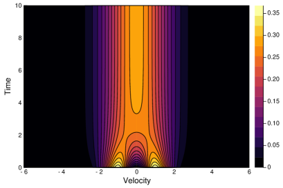
(a) Expectation value

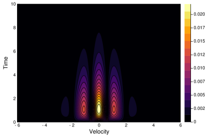
(b) Standard deviation

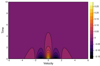
(c) Time derivative of mean value

Figure 2: Expectation value, its time derivatives, and standard deviation of particle distribution within $t,u\in[0,10]\times[-6,6]$ in the homogeneous relaxation problem.

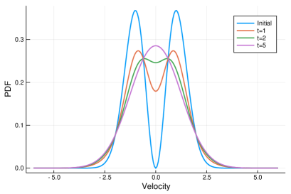
(a) Expectation value

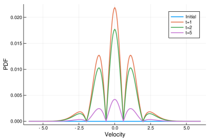
(b) Standard deviation

Figure 3: Expectation value and standard deviation of particle distribution over velocity space at different output time in the homogeneous relaxation problem.

Fig.2 presents the evolution of expectation and standard deviation of the particle distribution function over the entire phase space $\{t\times u\}$, and Fig.3 picks up some curves over velocity space at typical output time. As time goes, the initial bimodal particle distribution gradually approaches Maxwellian due to intermolecular collisions. The maximum value of standard deviation emerges around $t=1$, which is a local maximum given in Eq.(68). From a physical point of view, the random collision kernel results in more uncertainties where the distribution function is being reshaped by intermolecular interactions significantly. When $t>8$, with the distribution function being in a dynamical balance of a Maxwellian which is fully deterministic, the collision term has no explicit effects and the standard deviation approaches zero correspondingly. Fig.2(b) and 2(c) show the clear positive correlation between standard deviation and time derivative of expected value.

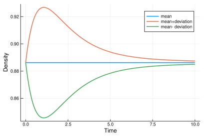
(a) Density

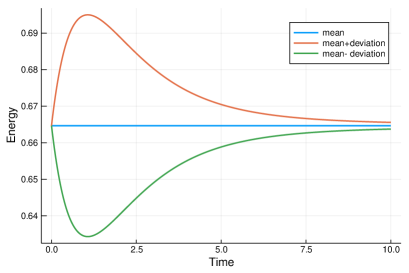
(b) Energy

Figure 4: Expectation values and standard deviations of macroscopic variables in the homogeneous relaxation problem.

Fig.4 presents the time evolution of macroscopic density and total energy. Since there is no contribution of inhomogeneous transport, the total density and energy expectations are conserved. The pattern of standard deviation here coincides with that of particle distribution function, with a local maximum value emerging around $t=1$. Since the formulas given in Eq.(68) are always symmetric in velocity space, the macroscopic fluid velocity always equals to zero, and the random collision kernel only affects the evolution of density and energy under the current initial condition.

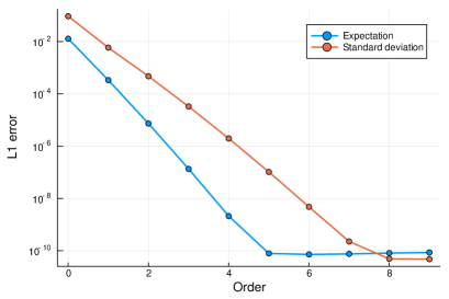
(a) $L_{1}$ error

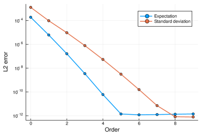
(b) $L_{2}$ error

Figure 5: Errors of expectation value and standard deviation of particle distribution function over the entire phase space $t,u\in[0,10]\times[-6,6]$ in the homogeneous relaxation problem.

To validate the current numerical scheme, Fig.5 presents its convergence results compared to theoretical solutions under different gPC expansion orders. From the results, the spectral convergence of stochastic Galerkin method is clearly identified.

4.2 Random collision kernel: normal shock structure

From now on we turn to spatially inhomogeneous problems. The first problem is the normal shock structure [muntz1969molecular]. Based on the reference frame of shock wave, the upstream and downstream gases are related with the well-known Rankine-Hugoniot relation,

$$\frac{\rho_{+}}{\rho_{-}}=\frac{(\gamma+1)\rm{Ma}^{2}}{(\gamma-1)\rm{Ma}^{2}+2},$$

$$\frac{U_{+}}{U_{-}}=\frac{(\gamma-1)\rm{Ma}^{2}+2}{(\gamma+1)\rm{Ma}^{2}},$$

$$\frac{T_{+}}{T_{-}}=\frac{((\gamma-1)\rm{Ma}^{2}+2)(2\gamma\rm{Ma}^{2}-\gamma+1)}{(\gamma+1)^{2}\rm{Ma}^{2}},$$

where $\gamma$ is the ratio of specific heat, and the upstream macroscopic density, velocity and temperature are denoted with $\{\rho_{-},U_{-},T_{-}\}$, and the downstream with $\{\rho_{+},U_{+},T_{+}\}$. The upstream Mach number is defined as the ratio between fluid velocity and sound speed, i.e.,

$$\rm{Ma}=\frac{U_{-}}{(\gamma/2\lambda_{-})^{1/2}}.$$

Note that now the speed of sound $c=(\gamma/2\lambda_{-})^{1/2}$ is larger than the most probable speed of molecule $(1/\lambda_{-})^{1/2}$. The randomness comes from the collision kernel, which follows Gaussian distribution in the random space,

$$\nu=1+0.05z.$$

In this case, the upstream flow quantities are chosen as references in the nondimensionalization. The physical domain is set as $x\in[-35,35]$ with 100 uniform cells, where the reference length $L_{0}$ is the mean free path of upstreaming gas. The truncated particle velocity space is $u\in[-12,12]$, which is discretized by 72 uniform quadrature points. The initial and boundary randomness in macroscopic variables and particle distribution function is set as zero, and the CFL number adopted is $0.95$. Both the stochastic Galerkin and hybrid Galerkin-collocation methods in Sec. 3.3 are used in the simulation, with 5th order gPC expansion and 9 Gaussian quadrature points employed. The Monte-Carlo simulation with 10000 samplings is also conducted for reference.

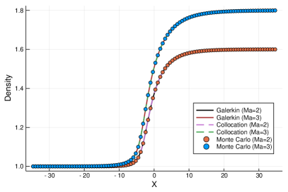
(a) Density

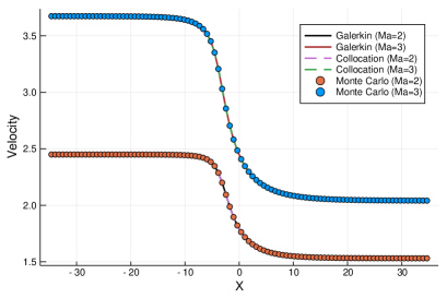
(b) Velocity

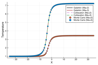
(c) Temperature

Figure 6: Expectations of density, velocity and temperature around normal shock wave.

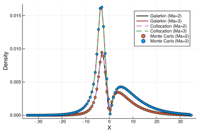
(a) Density

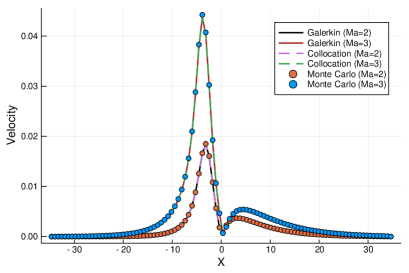
(b) Velocity

(c) Temperature

Figure 7: Standard deviations of density, velocity and temperature around normal shock wave.

Fig.6 and 7 present the numerical solutions from the three methods at different upstream Mach numbers $\rm Ma=2$ and $3$, and Table 1 shows their computational time costs. As shown, even with a a moderate number of samples, the Monte-Carlo method is much more time consuming than the intrusive stochastic methods. Due to the nonlinearity held in the collision operator of kinetic equation, the proposed hybrid method is more than ten times faster than the standard SG method, but maintains the same equivalent accuracy. At $\rm Ma=3$ the expected shock profile becomes wider than that of $\rm Ma=2$ due to the increasing momentum and energy transfers. From Fig.7, it is clear that the shock wave serves as a main source for uncertainties with significant intermolecular interactions inside it. Consistent with the behavior of expected flow quantities, the uncertainties at $\rm Ma=3$ are more significant and widely distributed than that of $\rm Ma=2$. Besides, it is noticeable that the uncertainties of all flow variables present a bimodal pattern inside the shock profile. Given the initial Rankine-Hugoniot jump relationship, the flow conditions at the center of shock $x=0$ are basically fixed, while the Mach number and collision kernel affect the shape and span of the shock profile. As shown in Fig.7, the upstream half of the shock wave seems to be more sensitive to the random collision kernel, resulting in a steeper distribution of uncertainties. After that, it approaches zero at the location of initial discontinuity and then arises again with a wider and moderate distribution at the downstream half. Of all the three macroscopic flow variables, the density profile contains considerable magnitude of uncertainty in the downstream part, while the temperature randomness is nearly located in the upstream half.

	Galerkin	Hybrid Galerkin-Collocation	Monte Carlo
Ma=2	5500	488	62575
Ma=3	13344	1180	140430

Table 1: The computational time costs in seconds of different numerical methods in normal shock structure problem.

4.3 Random initial input: multi-scale shock tube

The next case is Sod problem. The initial gas inside a one-dimensional tube $x\in[0,1]$ is set as,

$$\rho_{L},\quad U_{L}=0,\quad p_{L}=1.0,\quad x\leq 0.5,$$

$$\rho_{R}=0.125,\quad U_{R}=0,\quad p_{R}=0.1,\quad x>0.5,$$

with the corresponding particle distribution function being Maxwellian everywhere. We employ the variable hard-sphere (VHS) gas here, with its viscosity coefficient defined as,

$$\mu=\mu_{ref}\left(\frac{T}{T_{ref}}\right)^{\eta},$$

and the reference state is related with Knudsen number,

$$\mu_{ref}=\frac{5(\alpha+1)(\alpha+2)\sqrt{\pi}}{4\alpha(5-2\omega)(7-2\omega)}\mathrm{Kn}_{ref},$$

where the parameters $\{\alpha,\omega,\eta\}$ take the value $\{1,0.5,0.72\}$. The collision frequency is determined by

$$\nu=\frac{p}{\mu},$$

where $p$ is the pressure.

In the simulation, the physical domain is divided into 150 uniform cells, and the particle velocity space $u\in[-5,5]$ is discretized into 72 uniform quadrature points to update the distribution function. To test multi-scale performance of the current scheme, simulations are performed with different reference Knudsen numbers $\mathrm{Kn}_{ref}=1.0\times 10^{-4}$, $1.0\times 10^{-2}$, and $1.0$, with respect to typical continuum, transition, and free molecular flow regimes.

In this case, the uncertainties get involved into the stochastic system through random initial inputs. We consider two kinds of random distribution of the left-hand-side density, i.e. the normal and the uniform distributions over the random space,

$$(1)\rho_{L}\sim\mathcal{N}[\mu,\sigma^{2}],\ \mu=1.0,\ \sigma=0.0289,$$

$$(2)\rho_{L}\sim\mathcal{U}[a,b],\ a=0.95,\ b=1.05.$$

The parameters $\{\mu,\sigma,a,b\}$ are chosen in the way of keeping the same expectation and variance of initial density based on the probability theory. The stochastic Galerkin method is employed with 6th-order gPC expansion, while the reference solutions are conducted by the collocation method with 800 uniform cells.

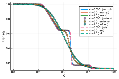
(a) Density

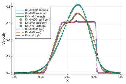
(b) Velocity

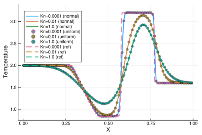
(c) Temperature

Figure 8: Expectations of density, velocity and temperature inside shock tube at different Knudsen numbers.

The numerical expectation solutions of macroscopic variables at $t=0.12$ are shown in Fig.8 and 9. In the continuum regime with $\mathrm{Kn}_{ref}=1.0\times 10^{-4}$, the molecular relaxation time is much smaller than the time step. As a result, the current scheme becomes a shock-capturing method due to limited resolution in space and time, and thus produces Euler solutions of the Riemann problem with wave-interaction structures. With increasing reference Knudsen number and molecular mean fee path, the degrees of freedom for individual particle free transport increase, and the flow physics changes significantly along with the enhanced transport phenomena. From $\mathrm{Kn}_{ref}=1.0\times 10^{-4}$ to $\mathrm{Kn}_{ref}=1.0$, a smooth transition is recovered from the Euler solutions of Riemann problem to collisionless Boltzmann solutions.

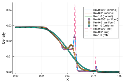
(a) Density

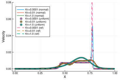
(b) Velocity

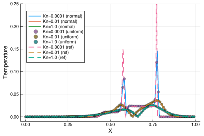
(c) Temperature

Figure 9: Standard deviations of density, velocity and temperature inside shock tube at different Knudsen numbers.

Fig.9 presents the standard deviations at the same output instant. Generally speaking, the uncertainties travel along with the wave structure of expectation values and present similar propagating patterns. At $\mathrm{Kn}_{ref}=1.0\times 10^{-4}$, structures such as rarefaction wave, contact discontinuity and shock also form inside the profiles of standard deviation. Given the uncertainty from initial gas density at the left hand side of the tube, it can be seen that the wave structures serves as other sources where the local maximums of variance emerge. Compared with the expectation value, it seems that the variance is more sensitive to physical discontinuities and holds finer-scale structures. As a result, the overshoots near contact discontinuity and shock cannot be well resolved by the shock-capturing scheme due to the limited resolution and there exist deviations between numerical and reference solutions, but it is clear that all the key structures are preserved. With increasing Knudsen numbers, the profiles of standard deviations get much smoother along with the wave-propagation structures inside the tube. At $\mathrm{Kn}_{ref}=1.0$, the density and velocity variance profiles show similar transition layers as their expectation values between upstream and downstream flow conditions.

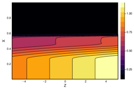
(a) Density

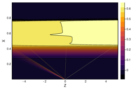
(b) Velocity

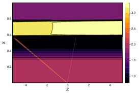
(c) Temperature

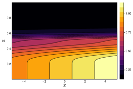
(d) Density

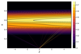
(e) Velocity

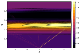
(f) Temperature

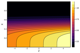
(g) Density

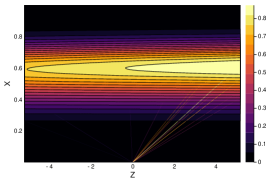
(h) Velocity

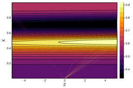
(i) Temperature

Figure 10: Evaluations of gPC expansions of macroscopic flow variables over random space inside shock tube at $\mathrm{Kn}_{ref}=0.001$ (first row), $\mathrm{Kn}_{ref}=0.01$ (second row) and $\mathrm{Kn}_{ref}=0.1$ (third row).

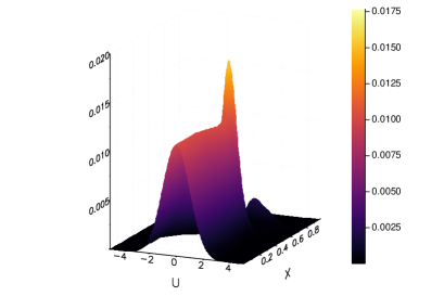
(b) Standard deviation

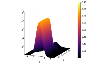
(c) Expectation

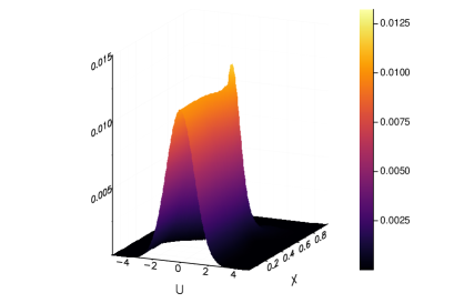
(d) Standard deviation

(e) Expectation

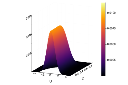
(f) Standard deviation

Figure 11: Expectation values and standard deviations of particle distribution function over velocity space inside shock tube at $\mathrm{Kn}_{ref}=0.001$ (first row), $\mathrm{Kn}_{ref}=0.01$ (second row) and $\mathrm{Kn}_{ref}=0.1$ (third row).

In Fig.10 we present the evaluation of gPC expansions of macroscopic flow variables over the phase space $\{x\times z\}$, where the expectation and standard deviation can be determined by integrating the contour value along the $z$-axis along with probability density. From the contours, we clearly see that it is the horizontal gradients that determine the variances of flow variables. With increasing Knudsen numbers, although the initial density keeps the same, the dominant physical mechanism in the gas dynamic system turns to particle transport from wave interaction. As a result, the enhanced transport phenomena lead significant dissipation along the random $z$-axis. Therefore, the magnitude of standard deviations reduces correspondingly. Moreover, with the correspondence between macroscopic and mesoscopic formulations, the stochastic kinetic scheme also provides us the chance to quantify the uncertainties in the evolution process of particle distribution function. Fig.11 presents the expectations and standard deviations of particle distribution function at different reference Knudsen numbers. As is shown, the overshoots in macroscopic standard deviations at $\mathrm{Kn}_{ref}=1.0\times 10^{-4}$ come from the uncertainties contained in the particle distribution function near the center of velocity space. From continuum to rarefied regimes, the randomness on particles get reduced and smoothed, resulting in gentle profiles of macroscopic quantities.

This test case clearly shows the consistency and distinction of propagation modes between expectation value and variance. It also illustrates the capacity of current scheme to simulate multi-scale flow physics and capture evolution of uncertainties in different regimes.

4.4 Random boundary condition: suddenly heating wall problem

The last case comes from [38, 39, 30]. The initial gas is uniformly and deterministically distributed inside the domain,

$$\rho_{0}=1,\ U_{0}=0,\ T_{0}=1,$$

with the particle distribution function being Maxwellian everywhere. From $t>0$, a heating wall is suddenly put on the left boundary of the domain, with the temperature being

$$T_{w}=2+0.4z,$$

where $z\sim\mathcal{U}[-1,1]$ is a random variable which follows uniform distribution.

In the simulation, the physical domain $x\in[0,0.5]$ is discretized by 200 uniform cells, and the particle velocity space is truncated into $u\in[-5,5]$ with 48 uniform quadrature points. The variable hard-sphere model is employed with the same parameter setup given in Sec. 4.3, and the Knudsen numbers in the reference state are chosen as $\mathrm{Kn}_{ref}=0.001$, $0.01$ and $0.1$. The Maxwell’s fully diffusive boundary is adopted at the left wall, and the right boundary is treated with extrapolation. The hybrid Galerkin-collocation method is employed with 6th-order gPC expansion and 11 Gauss collocation points, while the reference solutions are conducted by the collocation method with 800 uniform cells.

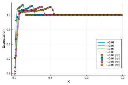
(a) $\mathbb{E}(\rho)$

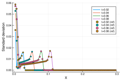
(b) $\mathbb{S}(\rho)$

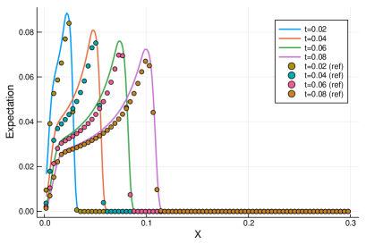
(c) $\mathbb{E}(U)$

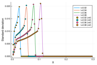
(d) $\mathbb{S}(U)$

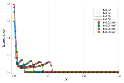
(e) $\mathbb{E}(T)$

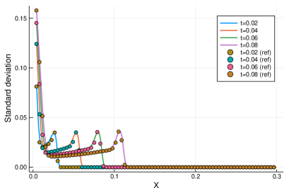
(f) $\mathbb{S}(T)$

Figure 12: Temporal evolutions of expectations and standard deviations of density (first row), velocity (second row) and temperature (third row) near the heat wall at $\mathrm{K}n_{ref}=0.001$.

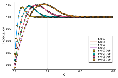
(a) $\mathbb{E}(\rho)$

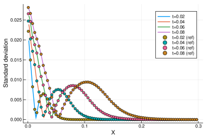
(b) $\mathbb{S}(\rho)$

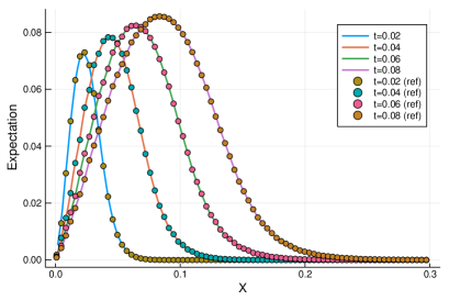
(c) $\mathbb{E}(U)$

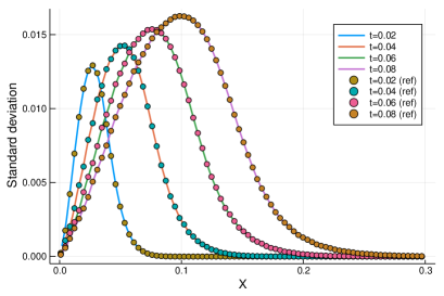
(d) $\mathbb{S}(U)$

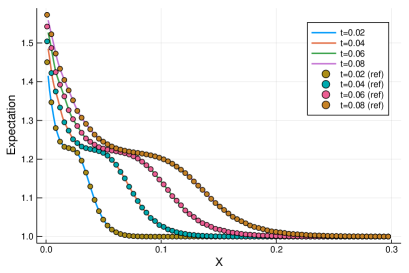
(e) $\mathbb{E}(T)$

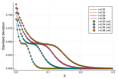
(f) $\mathbb{S}(T)$

Figure 14: Temporal evolutions of expectations and standard deviations of density (first row), velocity (second row) and temperature (third row) near the heat wall at $\mathrm{Kn}_{ref}=0.1$.

Fig.12, 13 and 14 present the expectation values and standard deviations of macroscopic gas density, velocity and temperature at different time instants $t=0.02$, $0.04$, $0.06$, and $0.08$. As is shown, with the heating wall, the gas temperature and pressure near the wall rise quickly, forming a shock wave propagating towards the bulk region. In Fig.12(a), (c) and (e), when $\mathrm{Kn}_{ref}=0.001$ with moderate viscosity and heat conductivity, the fine-scale structure cannot be resolved by the limited grid points, resulting in sharp discontinuity at the front head of shock wave, and the kinetic scheme becomes a shock capturing method. In this case, slight deviations exist between the numerical and reference solutions due to the limited resolution, but it is clear seen that all the key wave-interaction structures are preserved. With the increasing Knudsen number, the loose coupling between particle flight and collision leads to enhanced transport phenomena, and thus the diffusion process is accelerated and the steep shock discontinuity is smoothed into a milder profile. Compare Fig.14 with Fig.12, we see that the shock wave at $\mathrm{Kn}_{ref}=0.1$ travels twice faster than that at $\mathrm{Kn}_{ref}=0.001$.

Besides the evolution of mean field, the stochastic scheme provides us the opportunity to study the modes of uncertainty propagation from boundary to bulk region quantitatively. As shown in the second columns of Fig.12, 13 and 14, with randomly distributed boundary temperature, the near-wall gas holds the maximal variances of temperature and density, while the velocity variance is absent due to no-penetration condition across the wall. As time evolves, another local maximum of variance emerges and propagates rightwards inside the flow field along with the shock wave. For velocity and temperature, the propagating patterns of variances show clear similarity with expectation values. However, the standard deviation of density decreases linearly first and arise again towards the front of shock. The local mininum of variance locates near the starting point of intermediate regions with mitigatory temperature slope. At $\mathrm{Kn}_{ref}=0.001$ and $0.01$, due to the existence of viscosity, the traveling shock waves are gradually dissipated and the macroscopic flows are decelerated with smaller peak velocities. However, it seems that the strength of standard deviations is preserved and even enhanced as time goes, which indicates the accumulative effect for the propagation of uncertainties. Moreover, in all cases especially at $\mathrm{Kn}_{ref}=0.1$, it is noticed that the uncertainty travels a little faster than the mean field itself, which demonstrates the particular wave-propagation nature of uncertainty. It may be explained by the stronger sensitivity of uncertainty over mean field, which means the still gas will feel the existence of uncertainties in front of the shock.

With the one-to-one correspondence between hydrodynamic and mesoscopic formulations, the boundary heating process also evolves particles around the wall and passes uncertainties to the particle distribution function. Fig.15 presents the expectations and standard deviations of particle distribution function on the wall at different reference Knudsen numbers. Given the Maxwell’s diffusive boundary, the wall temperature defines the right half of particle distribution function with positive velocity $u>0$, while the left half is inherited from inner distribution function. As seen in Fig.15(e) and (f), it leads to a discontinuity in particle distribution at $\mathrm{Kn}_{ref}=0.1$, where the right half possesses much more significant uncertainties correspondingly. With increasing Knudsen number in Fig.15(a) to (d), frequent intermolecular interactions lead to equipartitions of energy, and thus the inner distribution functions are much closer to Maxwellian. As a result, the left and right parts of boundary particle distribution coincide with each other and the variances become symmetric with respect to zero velocity point. Fig.16, 17 and 18 show the standard deviations of particle distribution functions at different time instants and reference Knudsen numbers. Since the macroscopic velocity is very small in this heat diffusion problem, the variances basically keep symmetric along the velocity dimension, and the uncertainty waves propagate inside the phase space by reshaping the heights and widths of particle distribution functions.

5 Conclusion

Gas dynamics is a truly multiscale problem due to the large variations of gas density and characteristic length scales of the flow structures. Based on a kinetic model equation and its scale-dependent time evolving solution, a stochastic kinetic scheme with both standard stochastic Galerkin and hybrid Galerkin-collocation settings has been constructed in this paper, and both formulations allow for a unified flow simulation in all regimes. Based on multi-scale modeling, the solution algorithm is able to capture both equilibrium and non-equilibrium flow phenomena simultaneously in the flow field, and a continuous spectrum of cross-scale physics can be recovered along with the evolution of randomness. The asymptotic-preserving property of the scheme is validated through theoretical analysis and numerical tests. In the numerical experiments, for the first time non-equilibrium flow phenomena, such as the wave-propagation patterns of uncertainty from continuum to rarefied gas dynamics, could be clearly identified and quantitatively analyzed. The current scheme provides an efficient and accurate tool for the study of multi-scale non-equilibrium gas dynamics, and may help with the sensitivity analysis in design and applications of fluid machinery with uncertainty quantification. Its extension to multi-dimensional phase space and the analysis of the unified-preserving property [40] will be further considered in the future work.

(a) Expectation

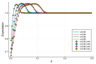
(a) $\mathbb{E}(\rho)$

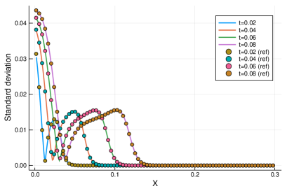
(b) $\mathbb{S}(\rho)$

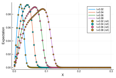
(c) $\mathbb{E}(U)$

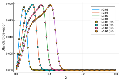
(d) $\mathbb{S}(U)$

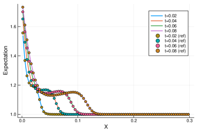
(e) $\mathbb{E}(T)$

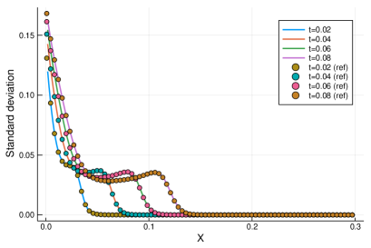
(f) $\mathbb{S}(T)$

Figure 13: Temporal evolutions of expectations and standard deviations of density (first row), velocity (second row) and temperature (third row) near the heat wall at $\mathrm{K}n_{ref}=0.01$.

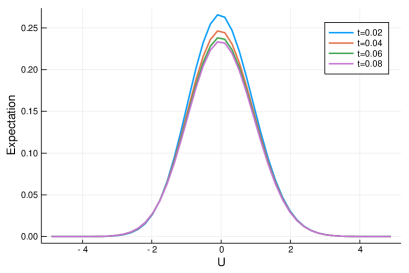
(a) $\mathbb{E}(f)$

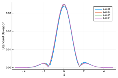
(b) $\mathbb{S}(f)$

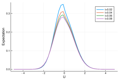
(c) $\mathbb{E}(f)$

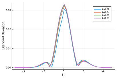
(d) $\mathbb{S}(f)$

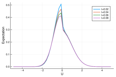
(e) $\mathbb{E}(f)$

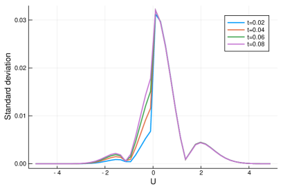
(f) $\mathbb{S}(f)$

Figure 15: Expectations and standard deviations of boundary particle distribution function at $\mathrm{Kn}_{ref}=0.001$ (first row), $\mathrm{Kn}_{ref}=0.01$ (second row) and $\mathrm{Kn}_{ref}=0.1$ (third row).

(a) $t=0.02$

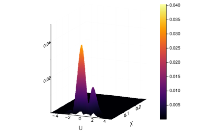
(b) $t=0.04$

(c) $t=0.06$

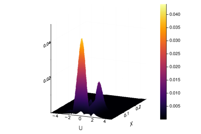
(d) $t=0.08$

Figure 16: Standard deviations of particle distribution function near the heat wall at $\mathrm{Kn}_{ref}=0.001$.

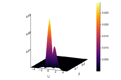
(a) $t=0.02$

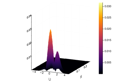
(b) $t=0.04$

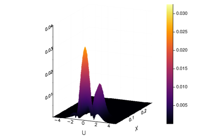
(c) $t=0.06$

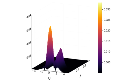
(d) $t=0.08$

Figure 17: Standard deviations of particle distribution function near the heat wall at $\mathrm{Kn}_{ref}=0.01$.

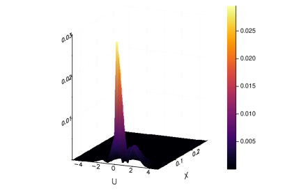
(a) $t=0.02$

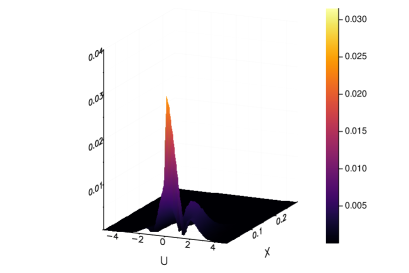
(b) $t=0.04$

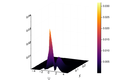
(c) $t=0.06$

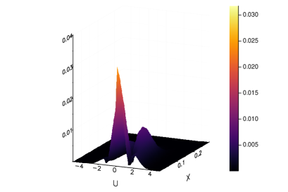
(d) $t=0.08$

Figure 18: Standard deviations of particle distribution function near the heat wall at $\mathrm{Kn}_{ref}=0.1$.

References

- [1] David Hilbert. Mathematical problems. Bulletin of the American Mathematical Society, 8(10):437–479, 1902.
- [2] Sydney Chapman and Thomas George Cowling. The mathematical theory of non-uniform gases: an account of the kinetic theory of viscosity, thermal conduction and diffusion in gases. Cambridge University Press, 1970.
- [3] Harold Grad. On the kinetic theory of rarefied gases. Communications on pure and applied mathematics, 2(4):331–407, 1949.
- [4] Byung Chan Eu. A modified moment method and irreversible thermodynamics. The Journal of Chemical Physics, 73(6):2958–2969, 1980.
- [5] C David Levermore. Moment closure hierarchies for kinetic theories. Journal of statistical Physics, 83(5-6):1021–1065, 1996.
- [6] Yoshio Sone. Kinetic theory and fluid dynamics. Springer Science & Business Media, 2012.
- [7] Manuel Torrilhon. Modeling nonequilibrium gas flow based on moment equations. Annual review of fluid mechanics, 48:429–458, 2016.
- [8] Shi Jin. Asymptotic preserving (ap) schemes for multiscale kinetic and hyperbolic equations: a review. Lecture notes for summer school on methods and models of kinetic theory (M&MKT), Porto Ercole (Grosseto, Italy), pages 177–216, 2010.
- [9] Pierre Degond, S Jin, and J Yuming. Mach-number uniform asymptotic-preserving gauge schemes for compressible flows. Bulletin-Institute of Mathematics Academia Sinica, 2(4):851, 2007.
- [10] Francis Filbet and Shi Jin. A class of asymptotic-preserving schemes for kinetic equations and related problems with stiff sources. Journal of Computational Physics, 229(20):7625–7648, 2010.
- [11] Christophe Berthon and Rodolphe Turpault. Asymptotic preserving hll schemes. Numerical methods for partial differential equations, 27(6):1396–1422, 2011.
- [12] Mohammed Lemou and Luc Mieussens. A new asymptotic preserving scheme based on micro-macro formulation for linear kinetic equations in the diffusion limit. SIAM Journal on Scientific Computing, 31(1):334–368, 2008.
- [13] Jian-Guo Liu and Luc Mieussens. Analysis of an asymptotic preserving scheme for linear kinetic equations in the diffusion limit. SIAM Journal on Numerical Analysis, 48(4):1474–1491, 2010.
- [14] Pierre Crispel, Pierre Degond, and Marie-Hélène Vignal. An asymptotic preserving scheme for the two-fluid euler–poisson model in the quasineutral limit. Journal of Computational Physics, 223(1):208–234, 2007.
- [15] Pierre Degond and Fabrice Deluzet. Asymptotic-preserving methods and multiscale models for plasma physics. Journal of Computational Physics, 336:429–457, 2017.
- [16] Kun Xu and Juan-Chen Huang. A unified gas-kinetic scheme for continuum and rarefied flows. Journal of Computational Physics, 229(20):7747–7764, 2010.
- [17] Chang Liu, Kun Xu, Quanhua Sun, and Qingdong Cai. A unified gas-kinetic scheme for continuum and rarefied flows iv: Full boltzmann and model equations. Journal of Computational Physics, 314:305–340, 2016.
- [18] Tianbai Xiao, Qingdong Cai, and Kun Xu. A well-balanced unified gas-kinetic scheme for multiscale flow transport under gravitational field. Journal of Computational Physics, 332:475 – 491, 2017.
- [19] Tianbai Xiao, Kun Xu, and Qingdong Cai. A unified gas-kinetic scheme for multiscale and multicomponent flow transport. Applied Mathematics and Mechanics, pages 1–18, 2019.
- [20] Luis Chacon, Guangye Chen, Dana A Knoll, C Newman, H Park, William Taitano, Jeff A Willert, and Geoffrey Womeldorff. Multiscale high-order/low-order (holo) algorithms and applications. Journal of Computational Physics, 330:21–45, 2017.
- [21] John Edward Lennard-Jones. On the determination of molecular fields. ii. from the equation of state of gas. Proc. Roy. Soc. A, 106:463–477, 1924.
- [22] Dongbin Xiu. Numerical methods for stochastic computations: a spectral method approach. Princeton university press, 2010.
- [23] Claudio Canuto and Alfio Quarteroni. Approximation results for orthogonal polynomials in sobolev spaces. Mathematics of Computation, 38(157):67–86, 1982.
- [24] Dongbin Xiu and George Em Karniadakis. Modeling uncertainty in flow simulations via generalized polynomial chaos. Journal of computational physics, 187(1):137–167, 2003.
- [25] David Gottlieb and Dongbin Xiu. Galerkin method for wave equations with uncertain coefficients. Commun. Comput. Phys, 3(2):505–518, 2008.
- [26] Shi Jin, Jian-Guo Liu, and Zheng Ma. Uniform spectral convergence of the stochastic galerkin method for the linear transport equations with random inputs in diffusive regime and a micro–macro decomposition-based asymptotic-preserving method. Research in the Mathematical Sciences, 4(1):15, 2017.
- [27] Lionel Mathelin, M Yousuff Hussaini, and Thomas A Zang. Stochastic approaches to uncertainty quantification in cfd simulations. Numerical Algorithms, 38(1-3):209–236, 2005.
- [28] Dongbin Xiu and Jan S Hesthaven. High-order collocation methods for differential equations with random inputs. SIAM Journal on Scientific Computing, 27(3):1118–1139, 2005.
- [29] Ivo Babuška, Fabio Nobile, and Raul Tempone. A stochastic collocation method for elliptic partial differential equations with random input data. SIAM Journal on Numerical Analysis, 45(3):1005–1034, 2007.
- [30] Jingwei Hu and Shi Jin. A stochastic galerkin method for the boltzmann equation with uncertainty. Journal of Computational Physics, 315:150–168, 2016.
- [31] Ruiwen Shu, Jingwei Hu, and Shi Jin. A stochastic galerkin method for the boltzmann equation with multi-dimensional random inputs using sparse wavelet bases. Numerical Mathematics: Theory, Methods and Applications, 10(2):465–488, 2017.
- [32] Jingwei Hu, Shi Jin, and Ruiwen Shu. On stochastic galerkin approximation of the nonlinear boltzmann equation with uncertainty in the fluid regime. preprint, 2019.
- [33] Clément Mouhot and Lorenzo Pareschi. Fast algorithms for computing the boltzmann collision operator. Mathematics of computation, 75(256):1833–1852, 2006.
- [34] Carlo Cercignani. The Boltzmann Equation and Its Applications. Springer, 1988.
- [35] Prabhu Lal Bhatnagar, Eugene P Gross, and Max Krook. A model for collision processes in gases. i. small amplitude processes in charged and neutral one-component systems. Physical review, 94(3):511, 1954.
- [36] Mikhail N Kogan. Rarefied Gas Dynamics. Plenum Press, 1969.
- [37] Tianbai Xiao, Kun Xu, Qingdong Cai, and Tiezheng Qian. An investigation of non-equilibrium heat transport in a gas system under external force field. International Journal of Heat and Mass Transfer, 126:362–379, 2018.
- [38] Kazuo Aoki, Yoshio Sone, Kenji Nishino, and Hiroshi Sugimoto. Numerical analysis of unsteady motion of a rarefied gas caused by sudden change of wall temperature with special interest in the propagation of discontinuity in the velocity distribution function. Mathematical Analysis of Phenomena in Fluid and Plasma Dynamics, 1991.
- [39] Francis Filbet. On deterministic approximation of the boltzmann equation in a bounded domain. Multiscale Modeling & Simulation, 10(3):792–817, 2012.
- [40] Zhaoli Guo, Jiequan Li, and Kun Xu. On unified preserving properties of kinetic schemes. arXiv preprint arXiv:1909.04923, 2019.