A Tutorial on Learning With Bayesian Networks

Abstract

A Bayesian network is a graphical model that encodes probabilistic relationships among variables of interest. When used in conjunction with statistical techniques, the graphical model has several advantages for data analysis. One, because the model encodes dependencies among all variables, it readily handles situations where some data entries are missing. Two, a Bayesian network can be used to learn causal relationships, and hence can be used to gain understanding about a problem domain and to predict the consequences of intervention. Three, because the model has both a causal and probabilistic semantics, it is an ideal representation for combining prior knowledge (which often comes in causal form) and data. Four, Bayesian statistical methods in conjunction with Bayesian networks offer an efficient and principled approach for avoiding the overfitting of data. In this paper, we discuss methods for constructing Bayesian networks from prior knowledge and summarize Bayesian statistical methods for using data to improve these models. With regard to the latter task, we describe methods for learning both the parameters and structure of a Bayesian network, including techniques for learning with incomplete data. In addition, we relate Bayesian-network methods for learning to techniques for supervised and unsupervised learning. We illustrate the graphical-modeling approach using a real-world case study.

1 Introduction

A Bayesian network is a graphical model for probabilistic relationships among a set of variables. Over the last decade, the Bayesian network has become a popular representation for encoding uncertain expert knowledge in expert systems (Heckerman et al., 1995a). More recently, researchers have developed methods for learning Bayesian networks from data. The techniques that have been developed are new and still evolving, but they have been shown to be remarkably effective for some data-analysis problems.

In this paper, we provide a tutorial on Bayesian networks and associated Bayesian techniques for extracting and encoding knowledge from data. There are numerous representations available for data analysis, including rule bases, decision trees, and artificial neural networks; and there are many techniques for data analysis such as density estimation, classification, regression, and clustering. So what do Bayesian networks and Bayesian methods have to offer? There are at least four answers.

One, Bayesian networks can readily handle incomplete data sets. For example, consider a classification or regression problem where two of the explanatory or input variables are strongly anti-correlated. This correlation is not a problem for standard supervised learning techniques, provided all inputs are measured in every case. When one of the inputs is not observed, however, most models will produce an inaccurate prediction, because they do not encode the correlation between the input variables. Bayesian networks offer a natural way to encode such dependencies.

Two, Bayesian networks allow one to learn about causal relationships. Learning about causal relationships are important for at least two reasons. The process is useful when we are trying to gain understanding about a problem domain, for example, during exploratory data analysis. In addition, knowledge of causal relationships allows us to make predictions in the presence of interventions. For example, a marketing analyst may want to know whether or not it is worthwhile to increase exposure of a particular advertisement in order to increase the sales of a product. To answer this question, the analyst can determine whether or not the advertisement is a cause for increased sales, and to what degree. The use of Bayesian networks helps to answer such questions even when no experiment about the effects of increased exposure is available.

Three, Bayesian networks in conjunction with Bayesian statistical techniques facilitate the combination of domain knowledge and data. Anyone who has performed a real-world analysis knows the importance of prior or domain knowledge, especially when data is scarce or expensive. The fact that some commercial systems (i.e., expert systems) can be built from prior knowledge alone is a testament to the power of prior knowledge. Bayesian networks have a causal semantics that makes the encoding of causal prior knowledge particularly straightforward. In addition, Bayesian networks encode the strength of causal relationships with probabilities. Consequently, prior knowledge and data can be combined with well-studied techniques from Bayesian statistics.

Four, Bayesian methods in conjunction with Bayesian networks and other types of models offers an efficient and principled approach for avoiding the over fitting of data. As we shall see, there is no need to hold out some of the available data for testing. Using the Bayesian approach, models can be “smoothed” in such a way that all available data can be used for training.

This tutorial is organized as follows. In Section 2, we discuss the Bayesian interpretation of probability and review methods from Bayesian statistics for combining prior knowledge with data. In Section 3, we describe Bayesian networks and discuss how they can be constructed from prior knowledge alone. In Section 4, we discuss algorithms for probabilistic inference in a Bayesian network. In Sections 5 and 6, we show how to learn the probabilities in a fixed Bayesian-network structure, and describe techniques for handling incomplete data including Monte-Carlo methods and the Gaussian approximation. In Sections 7 through 12, we show how to learn both the probabilities and structure of a Bayesian network. Topics discussed include methods for assessing priors for Bayesian-network structure and parameters, and methods for avoiding the overfitting of data including Monte-Carlo, Laplace, BIC, and MDL approximations. In Sections 13 and 14, we describe the relationships between Bayesian-network techniques and methods for supervised and unsupervised learning. In Section 15, we show how Bayesian networks facilitate the learning of causal relationships. In Section 16, we illustrate techniques discussed in the tutorial using a real-world case study. In Section 17, we give pointers to software and additional literature.

2 The Bayesian Approach to Probability and Statistics

To understand Bayesian networks and associated learning techniques, it is important to understand the Bayesian approach to probability and statistics. In this section, we provide an introduction to the Bayesian approach for those readers familiar only with the classical view.

In a nutshell, the Bayesian probability of an event $x$ is a person’s degree of belief in that event. Whereas a classical probability is a physical property of the world (e.g., the probability that a coin will land heads), a Bayesian probability is a property of the person who assigns the probability (e.g., your degree of belief that the coin will land heads). To keep these two concepts of probability distinct, we refer to the classical probability of an event as the true or physical probability of that event, and refer to a degree of belief in an event as a Bayesian or personal probability. Alternatively, when the meaning is clear, we refer to a Bayesian probability simply as a probability.

One important difference between physical probability and personal probability is that, to measure the latter, we do not need repeated trials. For example, imagine the repeated tosses of a sugar cube onto a wet surface. Every time the cube is tossed, its dimensions will change slightly. Thus, although the classical statistician has a hard time measuring the probability that the cube will land with a particular face up, the Bayesian simply restricts his or her attention to the next toss, and assigns a probability. As another example, consider the question: What is the probability that the Chicago Bulls will win the championship in 2001? Here, the classical statistician must remain silent, whereas the Bayesian can assign a probability (and perhaps make a bit of money in the process).

One common criticism of the Bayesian definition of probability is that probabilities seem arbitrary. Why should degrees of belief satisfy the rules of probability? On what scale should probabilities be measured? In particular, it makes sense to assign a probability of one (zero) to an event that will (not) occur, but what probabilities do we assign to beliefs that are not at the extremes? Not surprisingly, these questions have been studied intensely.

With regards to the first question, many researchers have suggested different sets of properties that should be satisfied by degrees of belief (e.g., Ramsey 1931, Cox 1946, Good 1950, Savage 1954, DeFinetti 1970). It turns out that each set of properties leads to the same rules: the rules of probability. Although each set of properties is in itself compelling, the fact that different sets all lead to the rules of probability provides a particularly strong argument for using probability to measure beliefs.

The answer to the question of scale follows from a simple observation: people find it fairly easy to say that two events are equally likely. For example, imagine a simplified wheel of fortune having only two regions (shaded and not shaded), such as the one illustrated in Figure 1. Assuming everything about the wheel as symmetric (except for shading), you should conclude that it is equally likely for the wheel to stop in any one position. From this judgment and the sum rule of probability (probabilities of mutually exclusive and collectively exhaustive sum to one), it follows that your probability that the wheel will stop in the shaded region is the percent area of the wheel that is shaded (in this case, 0.3).

This probability wheel now provides a reference for measuring your probabilities of other events. For example, what is your probability that Al Gore will run on the Democratic ticket in 2000? First, ask yourself the question: Is it more likely that Gore will run or that the wheel when spun will stop in the shaded region? If you think that it is more likely that Gore will run, then imagine another wheel where the shaded region is larger. If you think that it is more likely that the wheel will stop in the shaded region, then imagine another wheel where the shaded region is smaller. Now, repeat this process until you think that Gore running and the wheel stopping in the shaded region are equally likely. At this point, your probability that Gore will run is just the percent surface area of the shaded area on the wheel.

.

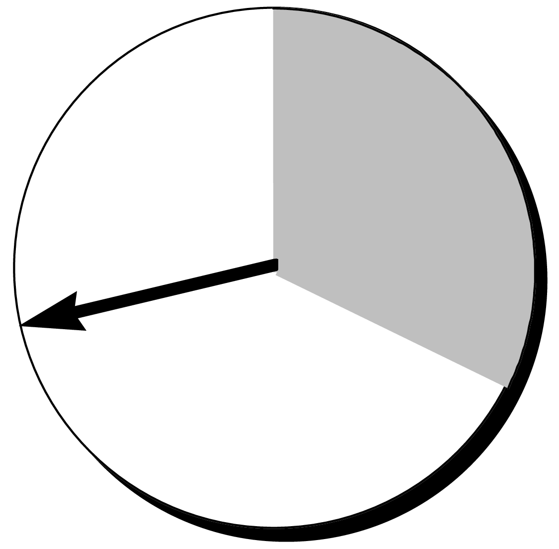
Figure 1: The probability wheel: a tool for assessing probabilities.

In general, the process of measuring a degree of belief is commonly referred to as a probability assessment. The technique for assessment that we have just described is one of many available techniques discussed in the Management Science, Operations Research, and Psychology literature. One problem with probability assessment that is addressed in this literature is that of precision. Can one really say that his or her probability for event $x$ is $0.601$ and not $0.599$? In most cases, no. Nonetheless, in most cases, probabilities are used to make decisions, and these decisions are not sensitive to small variations in probabilities. Well-established practices of sensitivity analysis help one to know when additional precision is unnecessary (e.g., Howard and Matheson, 1983). Another problem with probability assessment is that of accuracy. For example, recent experiences or the way a question is phrased can lead to assessments that do not reflect a person’s true beliefs (Tversky and Kahneman, 1974). Methods for improving accuracy can be found in the decision-analysis literature (e.g, Spetzler et al. (1975)).

Now let us turn to the issue of learning with data. To illustrate the Bayesian approach, consider a common thumbtack—one with a round, flat head that can be found in most supermarkets. If we throw the thumbtack up in the air, it will come to rest either on its point (heads) or on its head (tails). Suppose we flip the thumbtack $N+1$ times, making sure that the physical properties of the thumbtack and the conditions under which it is flipped remain stable over time. From the first $N$ observations, we want to determine the probability of heads on the $N+1$th toss.

In the classical analysis of this problem, we assert that there is some physical probability of heads, which is unknown. We estimate this physical probability from the $N$ observations using criteria such as low bias and low variance. We then use this estimate as our probability for heads on the $N+1$th toss. In the Bayesian approach, we also assert that there is some physical probability of heads, but we encode our uncertainty about this physical probability using (Bayesian) probabilities, and use the rules of probability to compute our probability of heads on the $N+1$th toss.

To examine the Bayesian analysis of this problem, we need some notation. We denote a variable by an upper-case letter (e.g., $X,Y,X_{i},\Theta$), and the state or value of a corresponding variable by that same letter in lower case (e.g., $x,y,x_{i},\theta$). We denote a set of variables by a bold-face upper-case letter (e.g., ${\bf X},{\bf Y},{\bf X}_{i}$). We use a corresponding bold-face lower-case letter (e.g., ${\bf x},{\bf y},{\bf x}_{i}$) to denote an assignment of state or value to each variable in a given set. We say that variable set ${\bf X}$ is in configuration ${\bf x}$. We use $p(X=x|\xi)$ (or $p(x|\xi)$ as a shorthand) to denote the probability that $X=x$ of a person with state of information $\xi$. We also use $p(x|\xi)$ to denote the probability distribution for $X$ (both mass functions and density functions). Whether $p(x|\xi)$ refers to a probability, a probability density, or a probability distribution will be clear from context. We use this notation for probability throughout the paper. A summary of all notation is given at the end of the chapter.

Returning to the thumbtack problem, we define $\Theta$ to be a variable whose values $\theta$ correspond to the possible true values of the physical probability. We sometimes refer to $\theta$ as a parameter. We express the uncertainty about $\Theta$ using the probability density function $p(\theta|\xi)$. In addition, we use $X_{l}$ to denote the variable representing the outcome of the $l$th flip, $l=1,\ldots,N+1$, and $D=\{X_{1}=x_{1},\ldots,X_{N}=x_{N}\}$ to denote the set of our observations. Thus, in Bayesian terms, the thumbtack problem reduces to computing $p(x_{N+1}|D,\xi)$ from $p(\theta|\xi)$.

To do so, we first use Bayes’ rule to obtain the probability distribution for $\Theta$ given $D$ and background knowledge $\xi$:

$$p(\theta|D,\xi)=\frac{p(\theta|\xi)\ p(D|\theta,\xi)}{p(D|\xi)}$$ (1)

where

$$p(D|\xi)=\int p(D|\theta,\xi)\ p(\theta|\xi)\ d\theta$$ (2)

Next, we expand the term $p(D|\theta,\xi)$. Both Bayesians and classical statisticians agree on this term: it is the likelihood function for binomial sampling. In particular, given the value of $\Theta$, the observations in $D$ are mutually independent, and the probability of heads (tails) on any one observation is $\theta$ ($1-\theta$). Consequently, Equation 1 becomes

$$p(\theta|D,\xi)=\frac{p(\theta|\xi)\ \theta^{h}\ (1-\theta)^{t}}{p(D|\xi)}$$ (3)

where $h$ and $t$ are the number of heads and tails observed in $D$, respectively. The probability distributions $p(\theta|\xi)$ and $p(\theta|D,\xi)$ are commonly referred to as the prior and posterior for $\Theta$, respectively. The quantities $h$ and $t$ are said to be sufficient statistics for binomial sampling, because they provide a summarization of the data that is sufficient to compute the posterior from the prior. Finally, we average over the possible values of $\Theta$ (using the expansion rule of probability) to determine the probability that the $N+1$th toss of the thumbtack will come up heads:

$$p(X_{N+1}=heads|D,\xi) = \int p(X_{N+1}=heads|\theta,\xi)\ p(\theta|D,\xi)\ d\theta$$ (4)

$$= \int\theta\ p(\theta|D,\xi)\ d\theta\equiv{\rm E}_{p(\theta|D,\xi)}(\theta)$$

where ${\rm E}_{p(\theta|D,\xi)}(\theta)$ denotes the expectation of $\theta$ with respect to the distribution $p(\theta|D,\xi)$.

To complete the Bayesian story for this example, we need a method to assess the prior distribution for $\Theta$. A common approach, usually adopted for convenience, is to assume that this distribution is a beta distribution:

$$p(\theta|\xi)={\rm Beta}(\theta|\alpha_{h},\alpha_{t})\equiv\frac{\Gamma(\alpha)}{\Gamma(\alpha_{h})\Gamma(\alpha_{t})}\theta^{\alpha_{h}-1}(1-\theta)^{\alpha_{t}-1}$$ (5)

where $\alpha_{h}>0$ and $\alpha_{t}>0$ are the parameters of the beta distribution, $\alpha=\alpha_{h}+\alpha_{t}$, and $\Gamma(\cdot)$ is the Gamma function which satisfies $\Gamma(x+1)=x\Gamma(x)$ and $\Gamma(1)=1$. The quantities $\alpha_{h}$ and $\alpha_{t}$ are often referred to as hyperparameters to distinguish them from the parameter $\theta$. The hyperparameters $\alpha_{h}$ and $\alpha_{t}$ must be greater than zero so that the distribution can be normalized. Examples of beta distributions are shown in Figure 2.

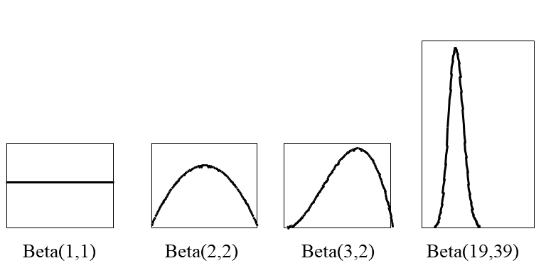
Figure 2: Several beta distributions.

The beta prior is convenient for several reasons. By Equation 3, the posterior distribution will also be a beta distribution:

$$p(\theta|D,\xi)=\frac{\Gamma(\alpha+N)}{\Gamma(\alpha_{h}+h)\Gamma(\alpha_{t}+t)}\theta^{\alpha_{h}+h-1}(1-\theta)^{\alpha_{t}+t-1}={\rm Beta}(\theta|\alpha_{h}+h,\alpha_{t}+t)$$ (6)

We say that the set of beta distributions is a conjugate family of distributions for binomial sampling. Also, the expectation of $\theta$ with respect to this distribution has a simple form:

$$\int\theta\ {\rm Beta}(\theta|\alpha_{h},\alpha_{t})\ d\theta=\frac{\alpha_{h}}{\alpha}$$ (7)

Hence, given a beta prior, we have a simple expression for the probability of heads in the $N+1$th toss:

$$p(X_{N+1}=heads|D,\xi)=\frac{\alpha_{h}+h}{\alpha+N}$$ (8)

Assuming $p(\theta|\xi)$ is a beta distribution, it can be assessed in a number of ways. For example, we can assess our probability for heads in the first toss of the thumbtack (e.g., using a probability wheel). Next, we can imagine having seen the outcomes of $k$ flips, and reassess our probability for heads in the next toss. From Equation 8, we have (for $k=1$)

$$p(X_{1}=heads|\xi)=\frac{\alpha_{h}}{\alpha_{h}+\alpha_{t}}\ \ \ \ \ p(X_{2}=heads|X_{1}=heads,\xi)=\frac{\alpha_{h}+1}{\alpha_{h}+\alpha_{t}+1}$$

Given these probabilities, we can solve for $\alpha_{h}$ and $\alpha_{t}$. This assessment technique is known as the method of imagined future data.

Another assessment method is based on Equation 6. This equation says that, if we start with a Beta$(0,0)$ prior and observe $\alpha_{h}$ heads and $\alpha_{t}$ tails, then our posterior (i.e., new prior) will be a Beta$(\alpha_{h},\alpha_{t})$ distribution. Recognizing that a Beta$(0,0)$ prior encodes a state of minimum information, we can assess $\alpha_{h}$ and $\alpha_{t}$ by determining the (possibly fractional) number of observations of heads and tails that is equivalent to our actual knowledge about flipping thumbtacks. Alternatively, we can assess $p(X_{1}=heads|\xi)$ and $\alpha$, which can be regarded as an equivalent sample size for our current knowledge. This technique is known as the method of equivalent samples. Other techniques for assessing beta distributions are discussed by Winkler (1967) and Chaloner and Duncan (1983).

Although the beta prior is convenient, it is not accurate for some problems. For example, suppose we think that the thumbtack may have been purchased at a magic shop. In this case, a more appropriate prior may be a mixture of beta distributions—for example,

$$p(\theta|\xi)=0.4\ {\rm Beta}(20,1)+0.4\ {\rm Beta}(1,20)+0.2\ {\rm Beta}(2,2)$$

where 0.4 is our probability that the thumbtack is heavily weighted toward heads (tails). In effect, we have introduced an additional hidden or unobserved variable $H$, whose states correspond to the three possibilities: (1) thumbtack is biased toward heads, (2) thumbtack is biased toward tails, and (3) thumbtack is normal; and we have asserted that $\theta$ conditioned on each state of $H$ is a beta distribution. In general, there are simple methods (e.g., the method of imagined future data) for determining whether or not a beta prior is an accurate reflection of one’s beliefs. In those cases where the beta prior is inaccurate, an accurate prior can often be assessed by introducing additional hidden variables, as in this example.

So far, we have only considered observations drawn from a binomial distribution. In general, observations may be drawn from any physical probability distribution:

$$p(x|\mbox{\boldmath$\theta$},\xi)=f(x,\mbox{\boldmath$\theta$})$$

where $f(x,\mbox{\boldmath$\theta$})$ is the likelihood function with parameters $\theta$. For purposes of this discussion, we assume that the number of parameters is finite. As an example, $X$ may be a continuous variable and have a Gaussian physical probability distribution with mean $\mu$ and variance $v$:

$$p(x|\mbox{\boldmath$\theta$},\xi)=(2\pi v)^{-1/2}\ e^{-(x-\mu)^{2}/2v}$$

where $\mbox{\boldmath$\theta$}=\{\mu,v\}$.

Regardless of the functional form, we can learn about the parameters given data using the Bayesian approach. As we have done in the binomial case, we define variables corresponding to the unknown parameters, assign priors to these variables, and use Bayes’ rule to update our beliefs about these parameters given data:

$$p(\mbox{\boldmath$\theta$}|D,\xi)=\frac{p(D|\mbox{\boldmath$\theta$},\xi)\ p(\mbox{\boldmath$\theta$}|\xi)}{p(D|\xi)}$$ (9)

We then average over the possible values of $\Theta$ to make predictions. For example,

$$p(x_{N+1}|D,\xi)=\int p(x_{N+1}|\mbox{\boldmath$\theta$},\xi)\ p(\mbox{\boldmath$\theta$}|D,\xi)\ d\mbox{\boldmath$\theta$}$$ (10)

For a class of distributions known as the exponential family, these computations can be done efficiently and in closed form. Members of this class include the binomial, multinomial, normal, Gamma, Poisson, and multivariate-normal distributions. Each member of this family has sufficient statistics that are of fixed dimension for any random sample, and a simple conjugate prior. Bernardo and Smith (pp. 436–442, 1994) have compiled the important quantities and Bayesian computations for commonly used members of the exponential family. Here, we summarize these items for multinomial sampling, which we use to illustrate many of the ideas in this paper.

In multinomial sampling, the observed variable $X$ is discrete, having $r$ possible states $x^{1},\ldots,x^{r}$. The likelihood function is given by

$$p(X=x^{k}|\mbox{\boldmath$\theta$},\xi)=\theta_{k},\ \ \ \ k=1,\ldots,r$$

where $\mbox{\boldmath$\theta$}=\{\theta_{2},\ldots,\theta_{r}\}$ are the parameters. (The parameter $\theta_{1}$ is given by $1-\sum_{k=2}^{r}\theta_{k}$.) In this case, as in the case of binomial sampling, the parameters correspond to physical probabilities. The sufficient statistics for data set $D=\{X_{1}=x_{1},\ldots,X_{N}=x_{N}\}$ are $\{N_{1},\ldots,N_{r}\}$, where $N_{i}$ is the number of times $X=x^{k}$ in $D$. The simple conjugate prior used with multinomial sampling is the Dirichlet distribution:

$$p(\mbox{\boldmath$\theta$}|\xi)={\rm Dir}(\mbox{\boldmath$\theta$}|\alpha_{1},\ldots,\alpha_{r})\equiv\frac{\Gamma(\alpha)}{\prod_{k=1}^{r}\Gamma(\alpha_{k})}\prod_{k=1}^{r}\theta_{k}^{\alpha_{k}-1}$$ (11)

where $\alpha=\sum_{i=1}^{r}\alpha_{k}$, and $\alpha_{k}>0,k=1,\ldots,r$. The posterior distribution $p(\mbox{\boldmath$\theta$}|D,\xi)={\rm Dir}(\mbox{\boldmath$\theta$}|\alpha_{1}+N_{1},\ldots,\alpha_{r}+N_{r})$. Techniques for assessing the beta distribution, including the methods of imagined future data and equivalent samples, can also be used to assess Dirichlet distributions. Given this conjugate prior and data set $D$, the probability distribution for the next observation is given by

$$p(X_{N+1}=x^{k}|D,\xi)=\int\theta_{k}\ {\rm Dir}(\mbox{\boldmath$\theta$}|\alpha_{1}+N_{1},\ldots,\alpha_{r}+N_{r})\ d\mbox{\boldmath$\theta$}=\frac{\alpha_{k}+N_{k}}{\alpha+N}$$ (12)

As we shall see, another important quantity in Bayesian analysis is the marginal likelihood or evidence $p(D|\xi)$. In this case, we have

$$p(D|\xi)=\frac{\Gamma(\alpha)}{\Gamma(\alpha+N)}\cdot\prod_{k=1}^{r}\frac{\Gamma(\alpha_{k}+N_{k})}{\Gamma(\alpha_{k})}$$ (13)

We note that the explicit mention of the state of knowledge $\xi$ is useful, because it reinforces the notion that probabilities are subjective. Nonetheless, once this concept is firmly in place, the notation simply adds clutter. In the remainder of this tutorial, we shall not mention $\xi$ explicitly.

In closing this section, we emphasize that, although the Bayesian and classical approaches may sometimes yield the same prediction, they are fundamentally different methods for learning from data. As an illustration, let us revisit the thumbtack problem. Here, the Bayesian “estimate” for the physical probability of heads is obtained in a manner that is essentially the opposite of the classical approach.

Namely, in the classical approach, $\theta$ is fixed (albeit unknown), and we imagine all data sets of size $N$ that may be generated by sampling from the binomial distribution determined by $\theta$. Each data set $D$ will occur with some probability $p(D|\theta)$ and will produce an estimate $\theta^{*}(D)$. To evaluate an estimator, we compute the expectation and variance of the estimate with respect to all such data sets:

$${\rm E}_{p(D|\theta)}(\theta^{*}) = \sum_{D}p(D|\theta)\ \theta^{*}(D)$$

$${\rm Var}_{p(D|\theta)}(\theta^{*}) = \sum_{D}p(D|\theta)\ (\theta^{*}(D)-{\rm E}_{p(D|\theta)}(\theta^{*}))^{2}$$ (14)

We then choose an estimator that somehow balances the bias ($\theta-{\rm E}_{p(D|\theta)}(\theta^{*})$) and variance of these estimates over the possible values for $\theta$. Finally, we apply this estimator to the data set that we actually observe. A commonly-used estimator is the maximum-likelihood (ML) estimator, which selects the value of $\theta$ that maximizes the likelihood $p(D|\theta)$. For binomial sampling, we have

$$\theta^{*}_{\rm ML}(D)=\frac{N_{k}}{\sum_{k=1}^{r}N_{k}}$$

For this (and other types) of sampling, the ML estimator is unbiased. That is, for all values of $\theta$, the ML estimator has zero bias. In addition, for all values of $\theta$, the variance of the ML estimator is no greater than that of any other unbiased estimator (see, e.g., Schervish, 1995).

In contrast, in the Bayesian approach, $D$ is fixed, and we imagine all possible values of $\theta$ from which this data set could have been generated. Given $\theta$, the “estimate” of the physical probability of heads is just $\theta$ itself. Nonetheless, we are uncertain about $\theta$, and so our final estimate is the expectation of $\theta$ with respect to our posterior beliefs about its value:

$${\rm E}_{p(\theta|D,\xi)}(\theta)=\int\theta\ p(\theta|D,\xi)\ d\theta$$ (15)

The expectations in Equations 2 and 15 are different and, in many cases, lead to different “estimates”. One way to frame this difference is to say that the classical and Bayesian approaches have different definitions for what it means to be a good estimator. Both solutions are “correct” in that they are self consistent. Unfortunately, both methods have their drawbacks, which has lead to endless debates about the merit of each approach. For example, Bayesians argue that it does not make sense to consider the expectations in Equation 2, because we only see a single data set. If we saw more than one data set, we should combine them into one larger data set. In contrast, classical statisticians argue that sufficiently accurate priors can not be assessed in many situations. The common view that seems to be emerging is that one should use whatever method that is most sensible for the task at hand. We share this view, although we also believe that the Bayesian approach has been under used, especially in light of its advantages mentioned in the introduction (points three and four). Consequently, in this paper, we concentrate on the Bayesian approach.

3 Bayesian Networks

So far, we have considered only simple problems with one or a few variables. In real learning problems, however, we are typically interested in looking for relationships among a large number of variables. The Bayesian network is a representation suited to this task. It is a graphical model that efficiently encodes the joint probability distribution (physical or Bayesian) for a large set of variables. In this section, we define a Bayesian network and show how one can be constructed from prior knowledge.

A Bayesian network for a set of variables ${\bf X}=\{X_{1},\ldots,X_{n}\}$ consists of (1) a network structure $S$ that encodes a set of conditional independence assertions about variables in ${\bf X}$, and (2) a set $P$ of local probability distributions associated with each variable. Together, these components define the joint probability distribution for ${\bf X}$. The network structure $S$ is a directed acyclic graph. The nodes in $S$ are in one-to-one correspondence with the variables ${\bf X}$. We use $X_{i}$ to denote both the variable and its corresponding node, and ${\bf Pa}_{i}$ to denote the parents of node $X_{i}$ in $S$ as well as the variables corresponding to those parents. The lack of possible arcs in $S$ encode conditional independencies. In particular, given structure $S$, the joint probability distribution for ${\bf X}$ is given by

$$p({\bf x})=\prod_{i=1}^{n}p(x_{i}|{\bf pa}_{i})$$ (16)

The local probability distributions $P$ are the distributions corresponding to the terms in the product of Equation 16. Consequently, the pair $(S,P)$ encodes the joint distribution $p({\bf x})$.

The probabilities encoded by a Bayesian network may be Bayesian or physical. When building Bayesian networks from prior knowledge alone, the probabilities will be Bayesian. When learning these networks from data, the probabilities will be physical (and their values may be uncertain). In subsequent sections, we describe how we can learn the structure and probabilities of a Bayesian network from data. In the remainder of this section, we explore the construction of Bayesian networks from prior knowledge. As we shall see in Section 10, this procedure can be useful in learning Bayesian networks as well.

To illustrate the process of building a Bayesian network, consider the problem of detecting credit-card fraud. We begin by determining the variables to model. One possible choice of variables for our problem is Fraud ($F$), Gas ($G$), Jewelry ($J$), Age ($A$), and Sex ($S$), representing whether or not the current purchase is fraudulent, whether or not there was a gas purchase in the last 24 hours, whether or not there was a jewelry purchase in the last 24 hours, and the age and sex of the card holder, respectively. The states of these variables are shown in Figure 3. Of course, in a realistic problem, we would include many more variables. Also, we could model the states of one or more of these variables at a finer level of detail. For example, we could let Age be a continuous variable.

This initial task is not always straightforward. As part of this task we must (1) correctly identify the goals of modeling (e.g., prediction versus explanation versus exploration), (2) identify many possible observations that may be relevant to the problem, (3) determine what subset of those observations is worthwhile to model, and (4) organize the observations into variables having mutually exclusive and collectively exhaustive states. Difficulties here are not unique to modeling with Bayesian networks, but rather are common to most approaches. Although there are no clean solutions, some guidance is offered by decision analysts (e.g., Howard and Matheson, 1983) and (when data are available) statisticians (e.g., Tukey, 1977).

In the next phase of Bayesian-network construction, we build a directed acyclic graph that encodes assertions of conditional independence. One approach for doing so is based on the following observations. From the chain rule of probability, we have

$$p({\bf x})=\prod_{i=1}^{n}p(x_{i}|x_{1},\ldots,x_{i-1})$$ (17)

Now, for every $X_{i}$, there will be some subset $\Pi_{i}\subseteq\{X_{1},\ldots,X_{i-1}\}$ such that $X_{i}$ and $\{X_{1},\ldots,X_{i-1}\}\setminus\Pi_{i}$ are conditionally independent given $\Pi_{i}$. That is, for any ${\bf x}$,

$$p(x_{i}|x_{1},\ldots,x_{i-1})=p(x_{i}|\pi_{i})$$ (18)

Combining Equations 17 and 18, we obtain

$$p({\bf x})=\prod_{i=1}^{n}p(x_{i}|\pi_{i})$$ (19)

Comparing Equations 16 and 19, we see that the variables sets $(\Pi_{1},\ldots,\Pi_{n})$ correspond to the Bayesian-network parents $({\bf Pa}_{1},\ldots,{\bf Pa}_{n})$, which in turn fully specify the arcs in the network structure $S$.

Consequently, to determine the structure of a Bayesian network we (1) order the variables somehow, and (2) determine the variables sets that satisfy Equation 18 for $i=1,\ldots,n$. In our example, using the ordering $(F,A,S,G,J)$, we have the conditional independencies

$$p(a|f) = p(a)$$

$$p(s|f,a) = p(s)$$

$$p(g|f,a,s) = p(g|f)$$

$$p(j|f,a,s,g) = p(j|f,a,s)$$ (20)

Thus, we obtain the structure shown in Figure 3.

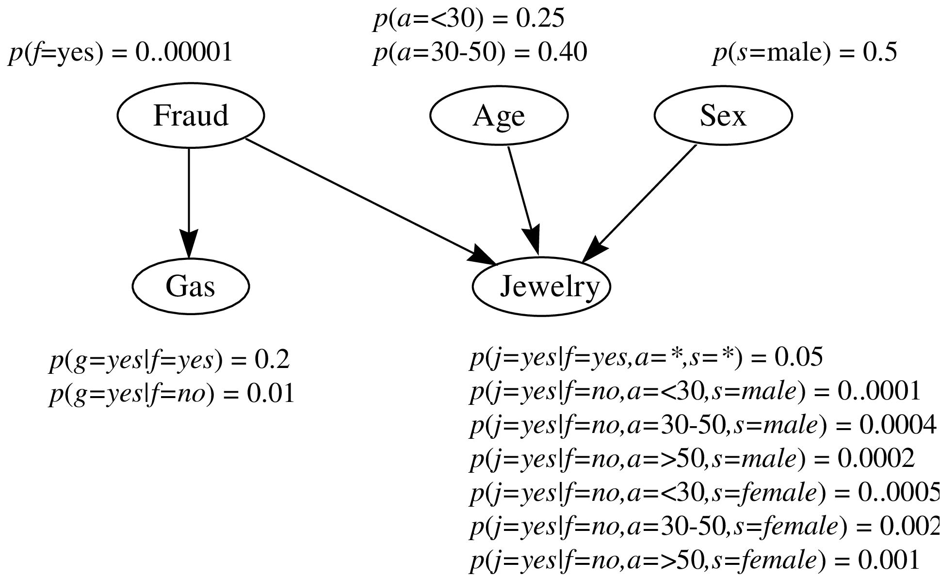
Figure 3: A Bayesian-network for detecting credit-card fraud. Arcs are drawn from cause to effect. The local probability distribution(s) associated with a node are shown adjacent to the node. An asterisk is a shorthand for “any state.”

This approach has a serious drawback. If we choose the variable order carelessly, the resulting network structure may fail to reveal many conditional independencies among the variables. For example, if we construct a Bayesian network for the fraud problem using the ordering $(J,G,S,A,F)$, we obtain a fully connected network structure. Thus, in the worst case, we have to explore $n!$ variable orderings to find the best one. Fortunately, there is another technique for constructing Bayesian networks that does not require an ordering. The approach is based on two observations: (1) people can often readily assert causal relationships among variables, and (2) causal relationships typically correspond to assertions of conditional dependence. In particular, to construct a Bayesian network for a given set of variables, we simply draw arcs from cause variables to their immediate effects. In almost all cases, doing so results in a network structure that satisfies the definition $Equation~{}\ref{eq:bn-def}$. For example, given the assertions that Fraud is a direct cause of Gas, and Fraud, Age, and Sex are direct causes of Jewelry, we obtain the network structure in Figure 3. The causal semantics of Bayesian networks are in large part responsible for the success of Bayesian networks as a representation for expert systems (Heckerman et al., 1995a). In Section 15, we will see how to learn causal relationships from data using these causal semantics.

In the final step of constructing a Bayesian network, we assess the local probability distribution(s) $p(x_{i}|{\bf pa}_{i})$. In our fraud example, where all variables are discrete, we assess one distribution for $X_{i}$ for every configuration of ${\bf Pa}_{i}$. Example distributions are shown in Figure 3.

Note that, although we have described these construction steps as a simple sequence, they are often intermingled in practice. For example, judgments of conditional independence and/or cause and effect can influence problem formulation. Also, assessments of probability can lead to changes in the network structure. Exercises that help one gain familiarity with the practice of building Bayesian networks can be found in Jensen (1996).

4 Inference in a Bayesian Network

Once we have constructed a Bayesian network (from prior knowledge, data, or a combination), we usually need to determine various probabilities of interest from the model. For example, in our problem concerning fraud detection, we want to know the probability of fraud given observations of the other variables. This probability is not stored directly in the model, and hence needs to be computed. In general, the computation of a probability of interest given a model is known as probabilistic inference. In this section we describe probabilistic inference in Bayesian networks.

Because a Bayesian network for ${\bf X}$ determines a joint probability distribution for ${\bf X}$, we can—in principle—use the Bayesian network to compute any probability of interest. For example, from the Bayesian network in Figure 3, the probability of fraud given observations of the other variables can be computed as follows:

$$p(f|a,s,g,j)=\frac{p(f,a,s,g,j)}{p(a,s,g,j)}=\frac{p(f,a,s,g,j)}{\sum_{f^{\prime}}p(f^{\prime},a,s,g,j)}$$ (21)

For problems with many variables, however, this direct approach is not practical. Fortunately, at least when all variables are discrete, we can exploit the conditional independencies encoded in a Bayesian network to make this computation more efficient. In our example, given the conditional independencies in Equation 3, Equation 21 becomes

$$p(f|a,s,g,j) = \frac{p(f)p(a)p(s)p(g|f)p(j|f,a,s)}{\sum_{f^{\prime}}p(f^{\prime})p(a)p(s)p(g|f^{\prime})p(j|f^{\prime},a,s)}$$

$$= \frac{p(f)p(g|f)p(j|f,a,s)}{\sum_{f^{\prime}}p(f^{\prime})p(g|f^{\prime})p(j|f^{\prime},a,s)}$$

Several researchers have developed probabilistic inference algorithms for Bayesian networks with discrete variables that exploit conditional independence roughly as we have described, although with different twists. For example, Howard and Matheson (1981), Olmsted (1983), and Shachter (1988) developed an algorithm that reverses arcs in the network structure until the answer to the given probabilistic query can be read directly from the graph. In this algorithm, each arc reversal corresponds to an application of Bayes’ theorem. Pearl (1986) developed a message-passing scheme that updates the probability distributions for each node in a Bayesian network in response to observations of one or more variables. Lauritzen and Spiegelhalter (1988), Jensen et al. (1990), and Dawid (1992) created an algorithm that first transforms the Bayesian network into a tree where each node in the tree corresponds to a subset of variables in ${\bf X}$. The algorithm then exploits several mathematical properties of this tree to perform probabilistic inference. Most recently, D’Ambrosio (1991) developed an inference algorithm that simplifies sums and products symbolically, as in the transformation from Equation 21 to 4. The most commonly used algorithm for discrete variables is that of Lauritzen and Spiegelhalter (1988), Jensen et al (1990), and Dawid (1992).

Methods for exact inference in Bayesian networks that encode multivariate-Gaussian or Gaussian-mixture distributions have been developed by Shachter and Kenley (1989) and Lauritzen (1992), respectively. These methods also use assertions of conditional independence to simplify inference. Approximate methods for inference in Bayesian networks with other distributions, such as the generalized linear-regression model, have also been developed (Saul et al., 1996; Jaakkola and Jordan, 1996).

Although we use conditional independence to simplify probabilistic inference, exact inference in an arbitrary Bayesian network for discrete variables is NP-hard (Cooper, 1990). Even approximate inference (for example, Monte-Carlo methods) is NP-hard (Dagum and Luby, 1993). The source of the difficulty lies in undirected cycles in the Bayesian-network structure—cycles in the structure where we ignore the directionality of the arcs. (If we add an arc from Age to Gas in the network structure of Figure 3, then we obtain a structure with one undirected cycle: $F-G-A-J-F$.) When a Bayesian-network structure contains many undirected cycles, inference is intractable. For many applications, however, structures are simple enough (or can be simplified sufficiently without sacrificing much accuracy) so that inference is efficient. For those applications where generic inference methods are impractical, researchers are developing techniques that are custom tailored to particular network topologies (Heckerman 1989; Suermondt and Cooper, 1991; Saul et al., 1996; Jaakkola and Jordan, 1996) or to particular inference queries (Ramamurthi and Agogino, 1988; Shachter et al., 1990; Jensen and Andersen, 1990; Darwiche and Provan, 1996).

5 Learning Probabilities in a Bayesian Network

In the next several sections, we show how to refine the structure and local probability distributions of a Bayesian network given data. The result is set of techniques for data analysis that combines prior knowledge with data to produce improved knowledge. In this section, we consider the simplest version of this problem: using data to update the probabilities of a given Bayesian network structure.

Recall that, in the thumbtack problem, we do not learn the probability of heads. Instead, we update our posterior distribution for the variable that represents the physical probability of heads. We follow the same approach for probabilities in a Bayesian network. In particular, we assume—perhaps from causal knowledge about the problem—that the physical joint probability distribution for ${\bf X}$ can be encoded in some network structure $S$. We write

$$p({\bf x}|\mbox{\boldmath$\theta$}_{s},S^{h})=\prod_{i=1}^{n}p(x_{i}|{\bf pa}_{i},\mbox{\boldmath$\theta$}_{i},S^{h})$$ (23)

where $\mbox{\boldmath$\theta$}_{i}$ is the vector of parameters for the distribution $p(x_{i}|{\bf pa}_{i},\mbox{\boldmath$\theta$}_{i},S^{h})$, $\mbox{\boldmath$\theta$}_{s}$ is the vector of parameters $(\mbox{\boldmath$\theta$}_{1},\ldots,\mbox{\boldmath$\theta$}_{n})$, and $S^{h}$ denotes the event (or “hypothesis” in statistics nomenclature) that the physical joint probability distribution can be factored according to $S$. In addition, we assume that we have a random sample $D=\{{\bf x}_{1},\ldots,{\bf x}_{N}\}$ from the physical joint probability distribution of ${\bf X}$. We refer to an element ${\bf x}_{l}$ of $D$ as a case. As in Section 2, we encode our uncertainty about the parameters $\mbox{\boldmath$\theta$}_{s}$ by defining a (vector-valued) variable $\Theta_{s}$, and assessing a prior probability density function $p(\mbox{\boldmath$\theta$}_{s}|S^{h})$. The problem of learning probabilities in a Bayesian network can now be stated simply: Given a random sample $D$, compute the posterior distribution $p(\mbox{\boldmath$\theta$}_{s}|D,S^{h})$.

We refer to the distribution $p(x_{i}|{\bf pa}_{i},\mbox{\boldmath$\theta$}_{i},S^{h})$, viewed as a function of $\mbox{\boldmath$\theta$}_{i}$, as a local distribution function. Readers familiar with methods for supervised learning will recognize that a local distribution function is nothing more than a probabilistic classification or regression function. Thus, a Bayesian network can be viewed as a collection of probabilistic classification/regression models, organized by conditional-independence relationships. Examples of classification/regression models that produce probabilistic outputs include linear regression, generalized linear regression, probabilistic neural networks (e.g., MacKay, 1992a, 1992b), probabilistic decision trees (e.g., Buntine, 1993; Friedman and Goldszmidt, 1996), kernel density estimation methods (Book, 1994), and dictionary methods (Friedman, 1995). In principle, any of these forms can be used to learn probabilities in a Bayesian network; and, in most cases, Bayesian techniques for learning are available. Nonetheless, the most studied models include the unrestricted multinomial distribution (e.g., Cooper and Herskovits, 1992), linear regression with Gaussian noise (e.g., Buntine, 1994; Heckerman and Geiger, 1996), and generalized linear regression (e.g., MacKay, 1992a and 1992b; Neal, 1993; and Saul et al., 1996).

In this tutorial, we illustrate the basic ideas for learning probabilities (and structure) using the unrestricted multinomial distribution. In this case, each variable $X_{i}\in{\bf X}$ is discrete, having $r_{i}$ possible values $x^{1}_{i},\ldots,x^{r_{i}}_{i}$, and each local distribution function is collection of multinomial distributions, one distribution for each configuration of ${\bf Pa}_{i}$. Namely, we assume

$$p(x^{k}_{i}|{\bf pa}_{i}^{j},\mbox{\boldmath$\theta$}_{i},S^{h})=\theta_{ijk}>0$$ (24)

where ${\bf pa}_{i}^{1},\ldots,{\bf pa}_{i}^{q_{i}}$ ($q_{i}=\prod_{X_{i}\in{\bf Pa}_{i}}r_{i}$) denote the configurations of ${\bf Pa}_{i}$, and $\mbox{\boldmath$\theta$}_{i}=((\theta_{ijk})_{k=2}^{r_{i}})_{j=1}^{q_{i}}$ are the parameters. (The parameter $\theta_{ij1}$ is given by $1-\sum_{k=2}^{r_{i}}\theta_{ijk}$.) For convenience, we define the vector of parameters

$$\mbox{\boldmath$\theta$}_{ij}=(\theta_{ij2},\ldots,\theta_{ijr_{i}})$$

for all $i$ and $j$. We use the term “unrestricted” to contrast this distribution with multinomial distributions that are low-dimensional functions of ${\bf Pa}_{i}$—for example, the generalized linear-regression model.

Given this class of local distribution functions, we can compute the posterior distribution $p(\mbox{\boldmath$\theta$}_{s}|D,S^{h})$ efficiently and in closed form under two assumptions. The first assumption is that there are no missing data in the random sample $D$. We say that the random sample $D$ is complete. The second assumption is that the parameter vectors $\mbox{\boldmath$\theta$}_{ij}$ are mutually independent. That is,

$$p(\mbox{\boldmath$\theta$}_{s}|S^{h})=\prod_{i=1}^{n}\prod_{j=1}^{q_{i}}p(\mbox{\boldmath$\theta$}_{ij}|S^{h})$$

We refer to this assumption, which was introduced by Spiegelhalter and Lauritzen (1990), as parameter independence.

Given that the joint physical probability distribution factors according to some network structure $S$, the assumption of parameter independence can itself be represented by a larger Bayesian-network structure. For example, the network structure in Figure 4 represents the assumption of parameter independence for ${\bf X}=\{X,Y\}$ ($X$, $Y$ binary) and the hypothesis that the network structure $X\rightarrow Y$ encodes the physical joint probability distribution for ${\bf X}$.

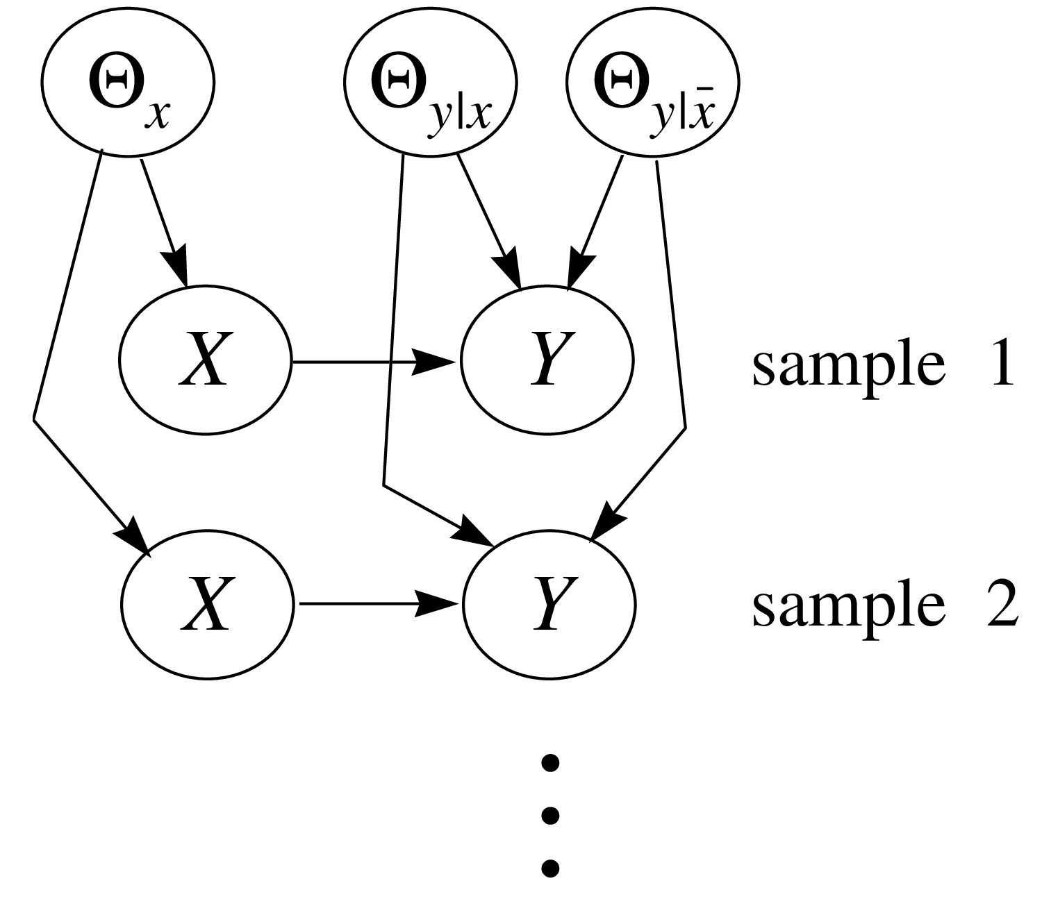
Figure 4: A Bayesian-network structure depicting the assumption of parameter independence for learning the parameters of the network structure $X\rightarrow Y$. Both variables $X$ and $Y$ are binary. We use $x$ and $\bar{x}$ to denote the two states of $X$, and $y$ and $\bar{y}$ to denote the two states of $Y$.

Under the assumptions of complete data and parameter independence, the parameters remain independent given a random sample:

$$p(\mbox{\boldmath$\theta$}_{s}|D,S^{h})=\prod_{i=1}^{n}\prod_{j=1}^{q_{i}}p(\mbox{\boldmath$\theta$}_{ij}|D,S^{h})$$ (25)

Thus, we can update each vector of parameters $\mbox{\boldmath$\theta$}_{ij}$ independently, just as in the one-variable case. Assuming each vector $\mbox{\boldmath$\theta$}_{ij}$ has the prior distribution Dir$(\mbox{\boldmath$\theta$}_{ij}|\alpha_{ij1},\ldots,\alpha_{ijr_{i}})$, we obtain the posterior distribution

$$p(\mbox{\boldmath$\theta$}_{ij}|D,S^{h})={\rm Dir}(\mbox{\boldmath$\theta$}_{ij}|\alpha_{ij1}+N_{ij1},\ldots,\alpha_{ijr_{i}}+N_{ijr_{i}})$$ (26)

where $N_{ijk}$ is the number of cases in $D$ in which $X_{i}=x_{i}^{k}$ and ${\bf Pa}_{i}={\bf pa}_{i}^{j}$.

As in the thumbtack example, we can average over the possible configurations of $\mbox{\boldmath$\theta$}_{s}$ to obtain predictions of interest. For example, let us compute $p({\bf x}_{N+1}|D,S^{h})$, where ${\bf x}_{N+1}$ is the next case to be seen after $D$. Suppose that, in case ${\bf x}_{N+1}$, $X_{i}=x_{i}^{k}$ and ${\bf Pa}_{i}={\bf pa}_{i}^{j}$, where $k$ and $j$ depend on $i$. Thus,

$$p({\bf x}_{N+1}|D,S^{h})={\rm E}_{p(\mbox{{\boldmath{\footnotesize$\theta$}}}_{s}|D,S^{h})}\left(\prod_{i=1}^{n}\theta_{ijk}\right)$$

To compute this expectation, we first use the fact that the parameters remain independent given $D$:

$$p({\bf x}_{N+1}|D,S^{h})=\int\prod_{i=1}^{n}\theta_{ijk}\ p(\mbox{\boldmath$\theta$}_{s}|D,S^{h})\ d\mbox{\boldmath$\theta$}_{s}=\prod_{i=1}^{n}\int\theta_{ijk}\ p(\mbox{\boldmath$\theta$}_{ij}|D,S^{h})\ d\mbox{\boldmath$\theta$}_{ij}$$

Then, we use Equation 12 to obtain

$$p({\bf x}_{N+1}|D,S^{h})=\prod_{i=1}^{n}\frac{\alpha_{ijk}+N_{ijk}}{\alpha_{ij}+N_{ij}}$$ (27)

where $\alpha_{ij}=\sum_{k=1}^{r_{i}}\alpha_{ijk}$ and $N_{ij}=\sum_{k=1}^{r_{i}}N_{ijk}$.

These computations are simple because the unrestricted multinomial distributions are in the exponential family. Computations for linear regression with Gaussian noise are equally straightforward (Buntine, 1994; Heckerman and Geiger, 1996).

6 Methods for Incomplete Data

Let us now discuss methods for learning about parameters when the random sample is incomplete (i.e., some variables in some cases are not observed). An important distinction concerning missing data is whether or not the absence of an observation is dependent on the actual states of the variables. For example, a missing datum in a drug study may indicate that a patient became too sick—perhaps due to the side effects of the drug—to continue in the study. In contrast, if a variable is hidden (i.e., never observed in any case), then the absence of this data is independent of state. Although Bayesian methods and graphical models are suited to the analysis of both situations, methods for handling missing data where absence is independent of state are simpler than those where absence and state are dependent. In this tutorial, we concentrate on the simpler situation only. Readers interested in the more complicated case should see Rubin (1978), Robins (1986), and Pearl (1995).

Continuing with our example using unrestricted multinomial distributions, suppose we observe a single incomplete case. Let ${\bf Y}\subset{\bf X}$ and ${\bf Z}\subset{\bf X}$ denote the observed and unobserved variables in the case, respectively. Under the assumption of parameter independence, we can compute the posterior distribution of $\mbox{\boldmath$\theta$}_{ij}$ for network structure $S$ as follows:

$$p(\mbox{\boldmath$\theta$}_{ij}|{\bf y},S^{h})=\sum_{{\bf z}}p({\bf z}|{\bf y},S^{h})\ p(\mbox{\boldmath$\theta$}_{ij}|{\bf y},{\bf z},S^{h})$$

$$=(1-p({\bf pa}_{i}^{j}|{\bf y},S^{h}))\left\{p(\mbox{\boldmath$\theta$}_{ij}|S^{h})\right\}+\sum_{k=1}^{r_{i}}p(x_{i}^{k},{\bf pa}_{i}^{j}|{\bf y},S^{h})\left\{p(\mbox{\boldmath$\theta$}_{ij}|x_{i}^{k},{\bf pa}_{i}^{j},S^{h})\right\}$$

(See Spiegelhalter and Lauritzen (1990) for a derivation.) Each term in curly brackets in Equation 6 is a Dirichlet distribution. Thus, unless both $X_{i}$ and all the variables in ${\bf Pa}_{i}$ are observed in case ${\bf y}$, the posterior distribution of $\mbox{\boldmath$\theta$}_{ij}$ will be a linear combination of Dirichlet distributions—that is, a Dirichlet mixture with mixing coefficients $(1-p({\bf pa}_{i}^{j}|{\bf y},S^{h}))$ and $p(x_{i}^{k},{\bf pa}_{i}^{j}|{\bf y},S^{h}),k=1,\ldots,r_{i}$.

When we observe a second incomplete case, some or all of the Dirichlet components in Equation 6 will again split into Dirichlet mixtures. That is, the posterior distribution for $\mbox{\boldmath$\theta$}_{ij}$ we become a mixture of Dirichlet mixtures. As we continue to observe incomplete cases, each missing values for ${\bf Z}$, the posterior distribution for $\mbox{\boldmath$\theta$}_{ij}$ will contain a number of components that is exponential in the number of cases. In general, for any interesting set of local likelihoods and priors, the exact computation of the posterior distribution for $\mbox{\boldmath$\theta$}_{s}$ will be intractable. Thus, we require an approximation for incomplete data.

6.1 Monte-Carlo Methods

One class of approximations is based on Monte-Carlo or sampling methods. These approximations can be extremely accurate, provided one is willing to wait long enough for the computations to converge.

In this section, we discuss one of many Monte-Carlo methods known as Gibbs sampling, introduced by Geman and Geman (1984). Given variables ${\bf X}=\{X_{1},\ldots,X_{n}\}$ with some joint distribution $p({\bf x})$, we can use a Gibbs sampler to approximate the expectation of a function $f({\bf x})$ with respect to $p({\bf x})$ as follows. First, we choose an initial state for each of the variables in ${\bf X}$ somehow (e.g., at random). Next, we pick some variable $X_{i}$, unassign its current state, and compute its probability distribution given the states of the other $n-1$ variables. Then, we sample a state for $X_{i}$ based on this probability distribution, and compute $f({\bf x})$. Finally, we iterate the previous two steps, keeping track of the average value of $f({\bf x})$. In the limit, as the number of cases approach infinity, this average is equal to ${\rm E}_{p({\bf x})}(f({\bf x}))$ provided two conditions are met. First, the Gibbs sampler must be irreducible: The probability distribution $p({\bf x})$ must be such that we can eventually sample any possible configuration of ${\bf X}$ given any possible initial configuration of ${\bf X}$. For example, if $p({\bf x})$ contains no zero probabilities, then the Gibbs sampler will be irreducible. Second, each $X_{i}$ must be chosen infinitely often. In practice, an algorithm for deterministically rotating through the variables is typically used. Introductions to Gibbs sampling and other Monte-Carlo methods—including methods for initialization and a discussion of convergence—are given by Neal (1993) and Madigan and York (1995).

To illustrate Gibbs sampling, let us approximate the probability density $p(\mbox{\boldmath$\theta$}_{s}|D,S^{h})$ for some particular configuration of $\mbox{\boldmath$\theta$}_{s}$, given an incomplete data set $D=\{{\bf y}_{1},\ldots,{\bf y}_{N}\}$ and a Bayesian network for discrete variables with independent Dirichlet priors. To approximate $p(\mbox{\boldmath$\theta$}_{s}|D,S^{h})$, we first initialize the states of the unobserved variables in each case somehow. As a result, we have a complete random sample $D_{c}$. Second, we choose some variable $X_{il}$ (variable $X_{i}$ in case $l$) that is not observed in the original random sample $D$, and reassign its state according to the probability distribution

$$p(x^{\prime}_{il}|D_{c}\setminus x_{il},S^{h})=\frac{p(x^{\prime}_{il},D_{c}\setminus x_{il}|S^{h})}{\sum_{x^{\prime\prime}_{il}}p(x^{\prime\prime}_{il},D_{c}\setminus x_{il}|S^{h})}$$

where $D_{c}\setminus x_{il}$ denotes the data set $D_{c}$ with observation $x_{il}$ removed, and the sum in the denominator runs over all states of variable $X_{il}$. As we shall see in Section 7, the terms in the numerator and denominator can be computed efficiently (see Equation 35). Third, we repeat this reassignment for all unobserved variables in $D$, producing a new complete random sample $D^{\prime}_{c}$. Fourth, we compute the posterior density $p(\mbox{\boldmath$\theta$}_{s}|D^{\prime}_{c},S^{h})$ as described in Equations 25 and 26. Finally, we iterate the previous three steps, and use the average of $p(\mbox{\boldmath$\theta$}_{s}|D^{\prime}_{c},S^{h})$ as our approximation.

6.2 The Gaussian Approximation

Monte-Carlo methods yield accurate results, but they are often intractable—for example, when the sample size is large. Another approximation that is more efficient than Monte-Carlo methods and often accurate for relatively large samples is the Gaussian approximation (e.g., Kass et al., 1988; Kass and Raftery, 1995).

The idea behind this approximation is that, for large amounts of data, $p(\mbox{\boldmath$\theta$}_{s}|D,S^{h})$ $\propto p(D|\mbox{\boldmath$\theta$}_{s},S^{h})\cdot p(\mbox{\boldmath$\theta$}_{s}|S^{h})$ can often be approximated as a multivariate-Gaussian distribution. In particular, let

$$g(\mbox{\boldmath$\theta$}_{s})\equiv\log(p(D|\mbox{\boldmath$\theta$}_{s},S^{h})\cdot p(\mbox{\boldmath$\theta$}_{s}|S^{h}))$$ (29)

Also, define $\tilde{\mbox{\boldmath$\theta$}_{s}}$ to be the configuration of $\mbox{\boldmath$\theta$}_{s}$ that maximizes $g(\mbox{\boldmath$\theta$}_{s})$. This configuration also maximizes $p(\mbox{\boldmath$\theta$}_{s}|D,S^{h})$, and is known as the maximum a posteriori (MAP) configuration of $\mbox{\boldmath$\theta$}_{s}$. Using a second degree Taylor polynomial of $g(\mbox{\boldmath$\theta$}_{s})$ about the $\tilde{\mbox{\boldmath$\theta$}_{s}}$ to approximate $g(\mbox{\boldmath$\theta$}_{s})$, we obtain

$$g(\mbox{\boldmath$\theta$}_{s})\approx g(\tilde{\mbox{\boldmath$\theta$}_{s}})-\frac{1}{2}(\mbox{\boldmath$\theta$}_{s}-\tilde{\mbox{\boldmath$\theta$}_{s}})A(\mbox{\boldmath$\theta$}_{s}-\tilde{\mbox{\boldmath$\theta$}_{s}})^{t}$$ (30)

where $(\mbox{\boldmath$\theta$}_{s}-\tilde{\mbox{\boldmath$\theta$}_{s}})^{t}$ is the transpose of row vector $(\mbox{\boldmath$\theta$}_{s}-\tilde{\mbox{\boldmath$\theta$}_{s}})$, and $A$ is the negative Hessian of $g(\mbox{\boldmath$\theta$}_{s})$ evaluated at $\tilde{\mbox{\boldmath$\theta$}_{s}}$. Raising $g(\mbox{\boldmath$\theta$}_{s})$ to the power of $e$ and using Equation 29, we obtain

$$p(\mbox{\boldmath$\theta$}_{s}|D,S^{h}) \propto p(D|\mbox{\boldmath$\theta$}_{s},S^{h})\ p(\mbox{\boldmath$\theta$}_{s}|S^{h})$$

$$\approx p(D|\tilde{\mbox{\boldmath$\theta$}_{s}},S^{h})\ p(\tilde{\mbox{\boldmath$\theta$}_{s}}|S^{h})\ \exp\{-\frac{1}{2}(\mbox{\boldmath$\theta$}_{s}-\tilde{\mbox{\boldmath$\theta$}_{s}})A(\mbox{\boldmath$\theta$}_{s}-\tilde{\mbox{\boldmath$\theta$}_{s}})^{t}\}$$

Hence, $p(\mbox{\boldmath$\theta$}_{s}|D,S^{h})$ is approximately Gaussian.

To compute the Gaussian approximation, we must compute $\tilde{\mbox{\boldmath$\theta$}_{s}}$ as well as the negative Hessian of $g(\mbox{\boldmath$\theta$}_{s})$ evaluated at $\tilde{\mbox{\boldmath$\theta$}_{s}}$. In the following section, we discuss methods for finding $\tilde{\mbox{\boldmath$\theta$}_{s}}$. Meng and Rubin (1991) describe a numerical technique for computing the second derivatives. Raftery (1995) shows how to approximate the Hessian using likelihood-ratio tests that are available in many statistical packages. Thiesson (1995) demonstrates that, for unrestricted multinomial distributions, the second derivatives can be computed using Bayesian-network inference.

6.3 The MAP and ML Approximations and the EM Algorithm

As the sample size of the data increases, the Gaussian peak will become sharper, tending to a delta function at the MAP configuration $\tilde{\mbox{\boldmath$\theta$}_{s}}$. In this limit, we do not need to compute averages or expectations. Instead, we simply make predictions based on the MAP configuration.

A further approximation is based on the observation that, as the sample size increases, the effect of the prior $p(\mbox{\boldmath$\theta$}_{s}|S^{h})$ diminishes. Thus, we can approximate $\tilde{\mbox{\boldmath$\theta$}_{s}}$ by the maximum maximum likelihood (ML) configuration of $\mbox{\boldmath$\theta$}_{s}$:

$$\hat{\mbox{\boldmath$\theta$}_{s}}=\arg\max_{\mbox{\boldmath$\theta$}_{s}}\left\{p(D|\mbox{\boldmath$\theta$}_{s},S^{h})\right\}$$

One class of techniques for finding a ML or MAP is gradient-based optimization. For example, we can use gradient ascent, where we follow the derivatives of $g(\mbox{\boldmath$\theta$}_{s})$ or the likelihood $p(D|\mbox{\boldmath$\theta$}_{s},S^{h})$ to a local maximum. Russell et al. (1995) and Thiesson (1995) show how to compute the derivatives of the likelihood for a Bayesian network with unrestricted multinomial distributions. Buntine (1994) discusses the more general case where the likelihood function comes from the exponential family. Of course, these gradient-based methods find only local maxima.

Another technique for finding a local ML or MAP is the expectation–maximization (EM) algorithm (Dempster et al., 1977). To find a local MAP or ML, we begin by assigning a configuration to $\mbox{\boldmath$\theta$}_{s}$ somehow (e.g., at random). Next, we compute the expected sufficient statistics for a complete data set, where expectation is taken with respect to the joint distribution for ${\bf X}$ conditioned on the assigned configuration of $\mbox{\boldmath$\theta$}_{s}$ and the known data $D$. In our discrete example, we compute

$${\rm E}_{p({\bf x}|D,\mbox{{\boldmath{\footnotesize$\theta$}}}_{s},S^{h})}(N_{ijk})=\sum_{l=1}^{N}p(x_{i}^{k},{\bf pa}_{i}^{j}|{\bf y}_{l},\mbox{\boldmath$\theta$}_{s},S^{h})$$ (32)

where ${\bf y}_{l}$ is the possibly incomplete $l$th case in $D$. When $X_{i}$ and all the variables in ${\bf Pa}_{i}$ are observed in case ${\bf x}_{l}$, the term for this case requires a trivial computation: it is either zero or one. Otherwise, we can use any Bayesian network inference algorithm to evaluate the term. This computation is called the expectation step of the EM algorithm.

Next, we use the expected sufficient statistics as if they were actual sufficient statistics from a complete random sample $D_{c}$. If we are doing an ML calculation, then we determine the configuration of $\mbox{\boldmath$\theta$}_{s}$ that maximize $p(D_{c}|\mbox{\boldmath$\theta$}_{s},S^{h})$. In our discrete example, we have

$$\theta_{ijk}=\frac{{\rm E}_{p({\bf x}|D,\mbox{{\boldmath{\footnotesize$\theta$}}}_{s},S^{h})}(N_{ijk})}{\sum_{k=1}^{r_{i}}{\rm E}_{p({\bf x}|D,\mbox{{\boldmath{\footnotesize$\theta$}}}_{s},S^{h})}(N_{ijk})}$$

If we are doing a MAP calculation, then we determine the configuration of $\mbox{\boldmath$\theta$}_{s}$ that maximizes $p(\mbox{\boldmath$\theta$}_{s}|D_{c},S^{h})$. In our discrete example, we have

$$\theta_{ijk}=\frac{\alpha_{ijk}+{\rm E}_{p({\bf x}|D,\mbox{{\boldmath{\footnotesize$\theta$}}}_{s},S^{h})}(N_{ijk})}{\sum_{k=1}^{r_{i}}(\alpha_{ijk}+{\rm E}_{p({\bf x}|D,\mbox{{\boldmath{\footnotesize$\theta$}}}_{s},S^{h})}(N_{ijk}))}$$

This assignment is called the maximization step of the EM algorithm. Dempster et al. (1977) showed that, under certain regularity conditions, iteration of the expectation and maximization steps will converge to a local maximum. The EM algorithm is typically applied when sufficient statistics exist (i.e., when local distribution functions are in the exponential family), although generalizations of the EM algroithm have been used for more complicated local distributions (see, e.g., Saul et al. 1996).

7 Learning Parameters and Structure

Now we consider the problem of learning about both the structure and probabilities of a Bayesian network given data.

Assuming we think structure can be improved, we must be uncertain about the network structure that encodes the physical joint probability distribution for ${\bf X}$. Following the Bayesian approach, we encode this uncertainty by defining a (discrete) variable whose states correspond to the possible network-structure hypotheses $S^{h}$, and assessing the probabilities $p(S^{h})$. Then, given a random sample $D$ from the physical probability distribution for ${\bf X}$, we compute the posterior distribution $p(S^{h}|D)$ and the posterior distributions $p(\mbox{\boldmath$\theta$}_{s}|D,S^{h})$, and use these distributions in turn to compute expectations of interest. For example, to predict the next case after seeing $D$, we compute

$$p({\bf x}_{N+1}|D)=\sum_{S^{h}}p(S^{h}|D)\int p({\bf x}_{N+1}|\mbox{\boldmath$\theta$}_{s},S^{h})\ p(\mbox{\boldmath$\theta$}_{s}|D,S^{h})\ d\mbox{\boldmath$\theta$}_{s}$$ (33)

In performing the sum, we assume that the network-structure hypotheses are mutually exclusive. We return to this point in Section 9.

The computation of $p(\mbox{\boldmath$\theta$}_{s}|D,S^{h})$ is as we have described in the previous two sections. The computation of $p(S^{h}|D)$ is also straightforward, at least in principle. From Bayes’ theorem, we have

$$p(S^{h}|D)=p(S^{h})\ p(D|S^{h})/p(D)$$ (34)

where $p(D)$ is a normalization constant that does not depend upon structure. Thus, to determine the posterior distribution for network structures, we need to compute the marginal likelihood of the data ($p(D|S^{h})$) for each possible structure.

We discuss the computation of marginal likelihoods in detail in Section 9. As an introduction, consider our example with unrestricted multinomial distributions, parameter independence, Dirichlet priors, and complete data. As we have discussed, when there are no missing data, each parameter vector $\mbox{\boldmath$\theta$}_{ij}$ is updated independently. In effect, we have a separate multi-sided thumbtack problem for every $i$ and $j$. Consequently, the marginal likelihood of the data is the just the product of the marginal likelihoods for each $i$–$j$ pair (given by Equation 13):

$$p(D|S^{h})=\prod_{i=1}^{n}\prod_{j=1}^{q_{i}}\frac{\Gamma(\alpha_{ij})}{\Gamma(\alpha_{ij}+N_{ij})}\cdot\prod_{k=1}^{r_{i}}\frac{\Gamma(\alpha_{ijk}+N_{ijk})}{\Gamma(\alpha_{ijk})}$$ (35)

This formula was first derived by Cooper and Herskovits (1992).

Unfortunately, the full Bayesian approach that we have described is often impractical. One important computation bottleneck is produced by the average over models in Equation 33. If we consider Bayesian-network models with $n$ variables, the number of possible structure hypotheses is more than exponential in $n$. Consequently, in situations where the user can not exclude almost all of these hypotheses, the approach is intractable.

Statisticians, who have been confronted by this problem for decades in the context of other types of models, use two approaches to address this problem: model selection and selective model averaging. The former approach is to select a “good” model (i.e., structure hypothesis) from among all possible models, and use it as if it were the correct model. The latter approach is to select a manageable number of good models from among all possible models and pretend that these models are exhaustive. These related approaches raise several important questions. In particular, do these approaches yield accurate results when applied to Bayesian-network structures? If so, how do we search for good models? And how do we decide whether or not a model is “good”?

The question of accuracy is difficult to answer in theory. Nonetheless, several researchers have shown experimentally that the selection of a single good hypothesis often yields accurate predictions (Cooper and Herskovits 1992; Aliferis and Cooper 1994; Heckerman et al., 1995b) and that model averaging using Monte-Carlo methods can sometimes be efficient and yield even better predictions (Madigan et al., 1996). These results are somewhat surprising, and are largely responsible for the great deal of recent interest in learning with Bayesian networks. In Sections 8 through 10, we consider different definitions of what is means for a model to be “good”, and discuss the computations entailed by some of these definitions. In Section 11, we discuss model search.

We note that model averaging and model selection lead to models that generalize well to new data. That is, these techniques help us to avoid the overfitting of data. As is suggested by Equation 33, Bayesian methods for model averaging and model selection are efficient in the sense that all cases in $D$ can be used to both smooth and train the model. As we shall see in the following two sections, this advantage holds true for the Bayesian approach in general.

8 Criteria for Model Selection

Most of the literature on learning with Bayesian networks is concerned with model selection. In these approaches, some criterion is used to measure the degree to which a network structure (equivalence class) fits the prior knowledge and data. A search algorithm is then used to find an equivalence class that receives a high score by this criterion. Selective model averaging is more complex, because it is often advantageous to identify network structures that are significantly different. In many cases, a single criterion is unlikely to identify such complementary network structures. In this section, we discuss criteria for the simpler problem of model selection. For a discussion of selective model averaging, see Madigan and Raftery (1994).

8.1 Relative Posterior Probability

A criterion that is often used for model selection is the log of the relative posterior probability $\log p(D,S^{h})=\log p(S^{h})+\log p(D|S^{h})$. The logarithm is used for numerical convenience. This criterion has two components: the log prior and the log marginal likelihood. In Section 9, we examine the computation of the log marginal likelihood. In Section 10.2, we discuss the assessment of network-structure priors. Note that our comments about these terms are also relevant to the full Bayesian approach.

The log marginal likelihood has the following interesting interpretation described by Dawid (1984). From the chain rule of probability, we have

$$\log p(D|S^{h})=\sum_{l=1}^{N}\log p({\bf x}_{l}|{\bf x}_{1},\ldots,{\bf x}_{l-1},S^{h})$$ (36)

The term $p({\bf x}_{l}|{\bf x}_{1},\ldots,{\bf x}_{l-1},S^{h})$ is the prediction for ${\bf x}_{l}$ made by model $S^{h}$ after averaging over its parameters. The log of this term can be thought of as the utility or reward for this prediction under the utility function $\log p({\bf x})$. Thus, a model with the highest log marginal likelihood (or the highest posterior probability, assuming equal priors on structure) is also a model that is the best sequential predictor of the data $D$ under the log utility function.

Dawid (1984) also notes the relationship between this criterion and cross validation. When using one form of cross validation, known as leave-one-out cross validation, we first train a model on all but one of the cases in the random sample—say, $V_{l}=\{{\bf x}_{1},\ldots,{\bf x}_{l-1},{\bf x}_{l+1},\ldots,{\bf x}_{N}\}$. Then, we predict the omitted case, and reward this prediction under some utility function. Finally, we repeat this procedure for every case in the random sample, and sum the rewards for each prediction. If the prediction is probabilistic and the utility function is $\log p({\bf x})$, we obtain the cross-validation criterion

$${\rm CV}(S^{h},D)=\sum_{l=1}^{N}\log p({\bf x}_{l}|V_{l},S^{h})$$ (37)

which is similar to Equation 36. One problem with this criterion is that training and test cases are interchanged. For example, when we compute $p({\bf x}_{1}|V_{1},S^{h})$ in Equation 37, we use ${\bf x}_{2}$ for training and ${\bf x}_{1}$ for testing. Whereas, when we compute $p({\bf x}_{2}|V_{2},S^{h})$, we use ${\bf x}_{1}$ for training and ${\bf x}_{2}$ for testing. Such interchanges can lead to the selection of a model that over fits the data (Dawid, 1984). Various approaches for attenuating this problem have been described, but we see from Equation 36 that the log-marginal-likelihood criterion avoids the problem altogether. Namely, when using this criterion, we never interchange training and test cases.

8.2 Local Criteria

Consider the problem of diagnosing an ailment given the observation of a set of findings. Suppose that the set of ailments under consideration are mutually exclusive and collectively exhaustive, so that we may represent these ailments using a single variable $A$. A possible Bayesian network for this classification problem is shown in Figure 5.

The posterior-probability criterion is global in the sense that it is equally sensitive to all possible dependencies. In the diagnosis problem, the posterior-probability criterion is just as sensitive to dependencies among the finding variables as it is to dependencies between ailment and findings. Assuming that we observe all (or perhaps all but a few) of the findings in $D$, a more reasonable criterion would be local in the sense that it ignores dependencies among findings and is sensitive only to the dependencies among the ailment and findings. This observation applies to all classification and regression problems with complete data.

One such local criterion, suggested by Spiegelhalter et al. (1993), is a variation on the sequential log-marginal-likelihood criterion:

$${\rm LC}(S^{h},D)=\sum_{l=1}^{N}\log p(a_{l}|{\bf F}_{l},D_{l},S^{h})$$ (38)

where $a_{l}$ and ${\bf F}_{l}$ denote the observation of the ailment $A$ and findings ${\bf F}$ in the $l$th case, respectively. In other words, to compute the $l$th term in the product, we train our model $S$ with the first $l-1$ cases, and then determine how well it predicts the ailment given the findings in the $l$th case. We can view this criterion, like the log-marginal-likelihood, as a form of cross validation where training and test cases are never interchanged.

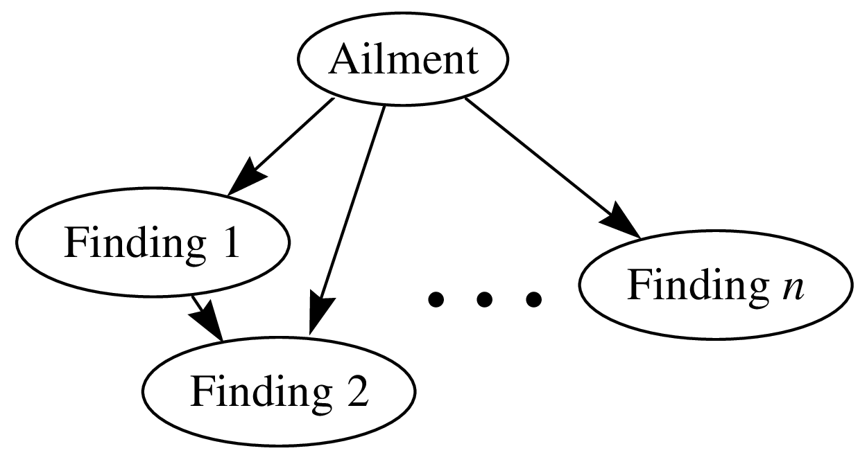
Figure 5: A Bayesian-network structure for medical diagnosis.

The log utility function has interesting theoretical properties, but it is sometimes inaccurate for real-world problems. In general, an appropriate reward or utility function will depend on the decision-making problem or problems to which the probabilistic models are applied. Howard and Matheson (1983) have collected a series of articles describing how to construct utility models for specific decision problems. Once we construct such utility models, we can use suitably modified forms of Equation 38 for model selection.

9 Computation of the Marginal Likelihood

As mentioned, an often-used criterion for model selection is the log relative posterior probability $\log p(D,S^{h})=\log p(S^{h})+\log p(D|S^{h})$. In this section, we discuss the computation of the second component of this criterion: the log marginal likelihood.

Given (1) local distribution functions in the exponential family, (2) mutual independence of the parameters $\mbox{\boldmath$\theta$}_{i}$, (3) conjugate priors for these parameters, and (4) complete data, the log marginal likelihood can be computed efficiently and in closed form. Equation 35 is an example for unrestricted multinomial distributions. Buntine (1994) and Heckerman and Geiger (1996) discuss the computation for other local distribution functions. Here, we concentrate on approximations for incomplete data.

The Monte-Carlo and Gaussian approximations for learning about parameters that we discussed in Section 6 are also useful for computing the marginal likelihood given incomplete data. One Monte-Carlo approach, described by Chib (1995) and Raftery (1996), uses Bayes’ theorem:

$$p(D|S^{h})=\frac{p(\mbox{\boldmath$\theta$}_{s}|S^{h})\ p(D|\mbox{\boldmath$\theta$}_{s},S^{h})}{p(\mbox{\boldmath$\theta$}_{s}|D,S^{h})}$$ (39)

For any configuration of $\mbox{\boldmath$\theta$}_{s}$, the prior term in the numerator can be evaluated directly. In addition, the likelihood term in the numerator can be computed using Bayesian-network inference. Finally, the posterior term in the denominator can be computed using Gibbs sampling, as we described in Section 6.1. Other, more sophisticated Monte-Carlo methods are described by DiCiccio et al. (1995).

As we have discussed, Monte-Carlo methods are accurate but computationally inefficient, especially for large data sets. In contrast, methods based on the Gaussian approximation are more efficient, and can be as accurate as Monte-Carlo methods on large data sets.

Recall that, for large amounts of data, $p(D|\mbox{\boldmath$\theta$}_{s},S^{h})\cdot p(\mbox{\boldmath$\theta$}_{s}|S^{h})$ can often be approximated as a multivariate-Gaussian distribution. Consequently,

$$p(D|S^{h})=\int p(D|\mbox{\boldmath$\theta$}_{s},S^{h})\ p(\mbox{\boldmath$\theta$}_{s}|S^{h})\ d\mbox{\boldmath$\theta$}_{s}$$ (40)

can be evaluated in closed form. In particular, substituting Equation 6.2 into Equation 40, integrating, and taking the logarithm of the result, we obtain the approximation:

$$\log p(D|S^{h})\approx\log p(D|\tilde{\mbox{\boldmath$\theta$}_{s}},S^{h})\ +\log p(\tilde{\mbox{\boldmath$\theta$}_{s}}|S^{h})\ +\frac{d}{2}\log(2\pi)-\frac{1}{2}\log|A|$$ (41)

where $d$ is the dimension of $g(\mbox{\boldmath$\theta$}_{s})$. For a Bayesian network with unrestricted multinomial distributions, this dimension is typically given by $\sum_{i=1}^{n}q_{i}(r_{i}-1)$. Sometimes, when there are hidden variables, this dimension is lower. See Geiger et al. (1996) for a discussion of this point.

This approximation technique for integration is known as Laplace’s method, and we refer to Equation 41 as the Laplace approximation. Kass et al. (1988) have shown that, under certain regularity conditions, relative errors in this approximation are $O(1/N)$, where $N$ is the number of cases in $D$. Thus, the Laplace approximation can be extremely accurate. For more detailed discussions of this approximation, see—for example—Kass et al. (1988) and Kass and Raftery (1995).

Although Laplace’s approximation is efficient relative to Monte-Carlo approaches, the computation of $|A|$ is nevertheless intensive for large-dimension models. One simplification is to approximate $|A|$ using only the diagonal elements of the Hessian $A$. Although in so doing, we incorrectly impose independencies among the parameters, researchers have shown that the approximation can be accurate in some circumstances (see, e.g., Becker and Le Cun, 1989, and Chickering and Heckerman, 1996). Another efficient variant of Laplace’s approximation is described by Cheeseman and Stutz (1995), who use the approximation in the AutoClass program for data clustering (see also Chickering and Heckerman, 1996.)

We obtain a very efficient (but less accurate) approximation by retaining only those terms in Equation 41 that increase with $N$: $\log p(D|\tilde{\mbox{\boldmath$\theta$}_{s}},S^{h})$, which increases linearly with $N$, and $\log|A|$, which increases as $d\log N$. Also, for large $N$, $\tilde{\mbox{\boldmath$\theta$}_{s}}$ can be approximated by the ML configuration of $\mbox{\boldmath$\theta$}_{s}$. Thus, we obtain

$$\log p(D|S^{h})\approx\log p(D|\hat{\mbox{\boldmath$\theta$}_{s}},S^{h})\ -\frac{d}{2}\log N$$ (42)

This approximation is called the Bayesian information criterion (BIC), and was first derived by Schwarz (1978).

The BIC approximation is interesting in several respects. First, it does not depend on the prior. Consequently, we can use the approximation without assessing a prior. Second, the approximation is quite intuitive. Namely, it contains a term measuring how well the parameterized model predicts the data ($\log p(D|\hat{\mbox{\boldmath$\theta$}_{s}},S^{h})$) and a term that punishes the complexity of the model ($d/2\ logN$). Third, the BIC approximation is exactly minus the Minimum Description Length (MDL) criterion described by Rissanen (1987). Thus, recalling the discussion in Section 9, we see that the marginal likelihood provides a connection between cross validation and MDL.

10 Priors

To compute the relative posterior probability of a network structure, we must assess the structure prior $p(S^{h})$ and the parameter priors $p(\mbox{\boldmath$\theta$}_{s}|S^{h})$ (unless we are using large-sample approximations such as BIC/MDL). The parameter priors $p(\mbox{\boldmath$\theta$}_{s}|S^{h})$ are also required for the alternative scoring functions discussed in Section 8. Unfortunately, when many network structures are possible, these assessments will be intractable. Nonetheless, under certain assumptions, we can derive the structure and parameter priors for many network structures from a manageable number of direct assessments. Several authors have discussed such assumptions and corresponding methods for deriving priors (Cooper and Herskovits, 1991, 1992; Buntine, 1991; Spiegelhalter et al., 1993; Heckerman et al., 1995b; Heckerman and Geiger, 1996). In this section, we examine some of these approaches.

10.1 Priors on Network Parameters

First, let us consider the assessment of priors for the model parameters. We consider the approach of Heckerman et al. (1995b) who address the case where the local distribution functions are unrestricted multinomial distributions and the assumption of parameter independence holds.

Their approach is based on two key concepts: independence equivalence and distribution equivalence. We say that two Bayesian-network structures for ${\bf X}$ are independence equivalent if they represent the same set of conditional-independence assertions for ${\bf X}$ (Verma and Pearl, 1990). For example, given ${\bf X}=\{X,Y,Z\}$, the network structures $X\rightarrow Y\rightarrow Z$, $X\leftarrow Y\rightarrow Z$, and $X\leftarrow Y\leftarrow Z$ represent only the independence assertion that $X$ and $Z$ are conditionally independent given $Y$. Consequently, these network structures are equivalent. As another example, a complete network structure is one that has no missing edge—that is, it encodes no assertion of conditional independence. When ${\bf X}$ contains $n$ variables, there are $n!$ possible complete network structures: one network structure for each possible ordering of the variables. All complete network structures for $p({\bf x})$ are independence equivalent. In general, two network structures are independence equivalent if and only if they have the same structure ignoring arc directions and the same v-structures (Verma and Pearl, 1990). A v-structure is an ordered tuple $(X,Y,Z)$ such that there is an arc from $X$ to $Y$ and from $Z$ to $Y$, but no arc between $X$ and $Z$.

The concept of distribution equivalence is closely related to that of independence equivalence. Suppose that all Bayesian networks for ${\bf X}$ under consideration have local distribution functions in the family ${\cal F}$. This is not a restriction, per se, because ${\cal F}$ can be a large family. We say that two Bayesian-network structures $S_{1}$ and $S_{2}$ for ${\bf X}$ are distribution equivalent with respect to (wrt) ${\cal F}$ if they represent the same joint probability distributions for ${\bf X}$—that is, if, for every $\mbox{\boldmath$\theta$}_{s1}$, there exists a $\mbox{\boldmath$\theta$}_{s2}$ such that $p({\bf x}|\mbox{\boldmath$\theta$}_{s1},S^{h}_{1})=p({\bf x}|\mbox{\boldmath$\theta$}_{s2},S^{h}_{2})$, and vice versa.

Distribution equivalence wrt some ${\cal F}$ implies independence equivalence, but the converse does not hold. For example, when ${\cal F}$ is the family of generalized linear-regression models, the complete network structures for $n\geq 3$ variables do not represent the same sets of distributions. Nonetheless, there are families ${\cal F}$—for example, unrestricted multinomial distributions and linear-regression models with Gaussian noise—where independence equivalence implies distribution equivalence wrt ${\cal F}$ (Heckerman and Geiger, 1996).

The notion of distribution equivalence is important, because if two network structures $S_{1}$ and $S_{2}$ are distribution equivalent wrt to a given ${\cal F}$, then the hypotheses associated with these two structures are identical—that is, $S^{h}_{1}=S^{h}_{2}$. Thus, for example, if $S_{1}$ and $S_{2}$ are distribution equivalent, then their probabilities must be equal in any state of information. Heckerman et al. (1995b) call this property hypothesis equivalence.

In light of this property, we should associate each hypothesis with an equivalence class of structures rather than a single network structure, and our methods for learning network structure should actually be interpreted as methods for learning equivalence classes of network structures (although, for the sake of brevity, we often blur this distinction). Thus, for example, the sum over network-structure hypotheses in Equation 33 should be replaced with a sum over equivalence-class hypotheses. An efficient algorithm for identifying the equivalence class of a given network structure can be found in Chickering (1995).

We note that hypothesis equivalence holds provided we interpret Bayesian-network structure simply as a representation of conditional independence. Nonetheless, stronger definitions of Bayesian networks exist where arcs have a causal interpretation (see Section 15). Heckerman et al. (1995b) and Heckerman (1995) argue that, although it is unreasonable to assume hypothesis equivalence when working with causal Bayesian networks, it is often reasonable to adopt a weaker assumption of likelihood equivalence, which says that the observational data can not help to discriminate two indepence equivalent network structures.

Now let us return to the main issue of this section: the derivation of priors from a manageable number of assessments. Geiger and Heckerman (1995) show that the assumptions of parameter independence and likelihood equivalence imply that the parameters for any complete network structure $S_{c}$ must have a Dirichlet distribution with constraints on the hyperparameters given by

$$\alpha_{ijk}=\alpha\ p(x_{i}^{k},{\bf pa}_{i}^{j}|S^{h}_{c})$$ (43)

where $\alpha$ is the user’s equivalent sample size,, and $p(x_{i}^{k},{\bf pa}_{i}^{j}|S^{h}_{c})$ is computed from the user’s joint probability distribution $p({\bf x}|S^{h}_{c})$. This result is rather remarkable, as the two assumptions leading to the constrained Dirichlet solution are qualitative.

To determine the priors for parameters of incomplete network structures, Heckerman et al. (1995b) use the assumption of parameter modularity, which says that if $X_{i}$ has the same parents in network structures $S_{1}$ and $S_{2}$, then

$$p(\mbox{\boldmath$\theta$}_{ij}|S^{h}_{1})=p(\mbox{\boldmath$\theta$}_{ij}|S^{h}_{2})$$

for $j=1,\ldots,q_{i}$. They call this property parameter modularity, because it says that the distributions for parameters $\mbox{\boldmath$\theta$}_{ij}$ depend only on the structure of the network that is local to variable $X_{i}$—namely, $X_{i}$ and its parents.

Given the assumptions of parameter modularity and parameter independence, it is a simple matter to construct priors for the parameters of an arbitrary network structure given the priors on complete network structures. In particular, given parameter independence, we construct the priors for the parameters of each node separately. Furthermore, if node $X_{i}$ has parents ${\bf Pa}_{i}$ in the given network structure, we identify a complete network structure where $X_{i}$ has these parents, and use Equation 43 and parameter modularity to determine the priors for this node. The result is that all terms $\alpha_{ijk}$ for all network structures are determined by Equation 43. Thus, from the assessments $\alpha$ and $p({\bf x}|S^{h}_{c})$, we can derive the parameter priors for all possible network structures. Combining Equation 43 with Equation 35, we obtain a model-selection criterion that assigns equal marginal likelihoods to independence equivalent network structures.

We can assess $p({\bf x}|S^{h}_{c})$ by constructing a Bayesian network, called a prior network, that encodes this joint distribution. Heckerman et al. (1995b) discuss the construction of this network.

10.2 Priors on Structures

Now, let us consider the assessment of priors on network-structure hypotheses. Note that the alternative criteria described in Section 8 can incorporate prior biases on network-structure hypotheses. Methods similar to those discussed in this section can be used to assess such biases.

The simplest approach for assigning priors to network-structure hypotheses is to assume that every hypothesis is equally likely. Of course, this assumption is typically inaccurate and used only for the sake of convenience. A simple refinement of this approach is to ask the user to exclude various hypotheses (perhaps based on judgments of of cause and effect), and then impose a uniform prior on the remaining hypotheses. We illustrate this approach in Section 12.

Buntine (1991) describes a set of assumptions that leads to a richer yet efficient approach for assigning priors. The first assumption is that the variables can be ordered (e.g., through a knowledge of time precedence). The second assumption is that the presence or absence of possible arcs are mutually independent. Given these assumptions, $n(n-1)/2$ probability assessments (one for each possible arc in an ordering) determines the prior probability of every possible network-structure hypothesis. One extension to this approach is to allow for multiple possible orderings. One simplification is to assume that the probability that an arc is absent or present is independent of the specific arc in question. In this case, only one probability assessment is required.

An alternative approach, described by Heckerman et al. (1995b) uses a prior network. The basic idea is to penalize the prior probability of any structure according to some measure of deviation between that structure and the prior network. Heckerman et al. (1995b) suggest one reasonable measure of deviation.

Madigan et al. (1995) give yet another approach that makes use of imaginary data from a domain expert. In their approach, a computer program helps the user create a hypothetical set of complete data. Then, using techniques such as those in Section 7, they compute the posterior probabilities of network-structure hypotheses given this data, assuming the prior probabilities of hypotheses are uniform. Finally, they use these posterior probabilities as priors for the analysis of the real data.

11 Search Methods

In this section, we examine search methods for identifying network structures with high scores by some criterion. Consider the problem of finding the best network from the set of all networks in which each node has no more than $k$ parents. Unfortunately, the problem for $k>1$ is NP-hard even when we use the restrictive prior given by Equation 43 (Chickering et al. 1995). Thus, researchers have used heuristic search algorithms, including greedy search, greedy search with restarts, best-first search, and Monte-Carlo methods.

One consolation is that these search methods can be made more efficient when the model-selection criterion is separable. Given a network structure for domain ${\bf X}$, we say that a criterion for that structure is separable if it can be written as a product of variable-specific criteria:

$${\rm C}(S^{h},D)=\prod_{i=1}^{n}\ c(X_{i},{\bf Pa}_{i},D_{i})$$ (44)

where $D_{i}$ is the data restricted to the variables $X_{i}$ and ${\bf Pa}_{i}$. An example of a separable criterion is the BD criterion (Equations 34 and 35) used in conjunction with any of the methods for assessing structure priors described in Section 10.

Most of the commonly used search methods for Bayesian networks make successive arc changes to the network, and employ the property of separability to evaluate the merit of each change. The possible changes that can be made are easy to identify. For any pair of variables, if there is an arc connecting them, then this arc can either be reversed or removed. If there is no arc connecting them, then an arc can be added in either direction. All changes are subject to the constraint that the resulting network contains no directed cycles. We use $E$ to denote the set of eligible changes to a graph, and $\Delta(e)$ to denote the change in log score of the network resulting from the modification $e\in E$. Given a separable criterion, if an arc to $X_{i}$ is added or deleted, only $c(X_{i},{\bf Pa}_{i},D_{i})$ need be evaluated to determine $\Delta(e)$. If an arc between $X_{i}$ and $X_{j}$ is reversed, then only $c(X_{i},{\bf Pa}_{i},D_{i})$ and $c(X_{j},\Pi_{j},D_{j})$ need be evaluated.

One simple heuristic search algorithm is greedy search. First, we choose a network structure. Then, we evaluate $\Delta(e)$ for all $e\in E$, and make the change $e$ for which $\Delta(e)$ is a maximum, provided it is positive. We terminate search when there is no $e$ with a positive value for $\Delta(e)$. When the criterion is separable, we can avoid recomputing all terms $\Delta(e)$ after every change. In particular, if neither $X_{i}$, $X_{j}$, nor their parents are changed, then $\Delta(e)$ remains unchanged for all changes $e$ involving these nodes as long as the resulting network is acyclic. Candidates for the initial graph include the empty graph, a random graph, and a prior network.

A potential problem with any local-search method is getting stuck at a local maximum. One method for escaping local maxima is greedy search with random restarts. In this approach, we apply greedy search until we hit a local maximum. Then, we randomly perturb the network structure, and repeat the process for some manageable number of iterations.

Another method for escaping local maxima is simulated annealing. In this approach, we initialize the system at some temperature $T_{0}$. Then, we pick some eligible change $e$ at random, and evaluate the expression $p=\exp(\Delta(e)/T_{0})$. If $p>1$, then we make the change $e$; otherwise, we make the change with probability $p$. We repeat this selection and evaluation process $\alpha$ times or until we make $\beta$ changes. If we make no changes in $\alpha$ repetitions, then we stop searching. Otherwise, we lower the temperature by multiplying the current temperature $T_{0}$ by a decay factor $0<\gamma<1$, and continue the search process. We stop searching if we have lowered the temperature more than $\delta$ times. Thus, this algorithm is controlled by five parameters: $T_{0},\alpha,\beta,\gamma$ and $\delta$. To initialize this algorithm, we can start with the empty graph, and make $T_{0}$ large enough so that almost every eligible change is made, thus creating a random graph. Alternatively, we may start with a lower temperature, and use one of the initialization methods described for local search.

Another method for escaping local maxima is best-first search (e.g., Korf, 1993). In this approach, the space of all network structures is searched systematically using a heuristic measure that determines the next best structure to examine. Chickering (1996b) has shown that, for a fixed amount of computation time, greedy search with random restarts produces better models than does best-first search.

One important consideration for any search algorithm is the search space. The methods that we have described search through the space of Bayesian-network structures. Nonetheless, when the assumption of hypothesis equivalence holds, one can search through the space of network-structure equivalence classes. One benefit of the latter approach is that the search space is smaller. One drawback of the latter approach is that it takes longer to move from one element in the search space to another. Work by Spirtes and Meek (1995) and Chickering (1996) confirm these observations experimentally. Unfortunately, no comparisons are yet available that determine whether the benefits of equivalence-class search outweigh the costs.

12 A Simple Example

Before we move on to other issues, let us step back and look at our overall approach. In a nutshell, we can construct both structure and parameter priors by constructing a Bayesian network (the prior network) along with additional assessments such as an equivalent sample size and causal constraints. We then use either Bayesian model selection, selective model averaging, or full model averaging to obtain one or more networks for prediction and/or explanation. In effect, we have a procedure for using data to improve the structure and probabilities of an initial Bayesian network.

Here, we present two artificial examples to illustrate this process. Consider again the problem of fraud detection from Section 3. Suppose we are given the data set $D$ in Table 1, and we want to predict the next case—that is, compute $p({\bf x}_{N+1}|D)$. Let us assert that only two network-structure hypotheses have appreciable probability: the hypothesis corresponding to the network structure in Figure 3 ($S_{1}$), and the hypothesis corresponding to the same structure with an arc added from Age to Gas ($S_{2}$). Furthermore, let us assert that these two hypotheses are equally likely—that is, $p(S^{h}_{1})=p(S^{h}_{2})=0.5$. In addition, let us use the parameter priors given by Equation 43, where $\alpha=10$ and $p({\bf x}|S^{h}_{c})$ is given by the prior network in Figure 3. Using Equations 34 and 35, we obtain $p(S^{h}_{1}|D)=0.26$ and $p(S^{h}_{2}|D)=0.74$. Because we have only two models to consider, we can model average according to Equation 33:

$$p({\bf x}_{N+1}|D)=0.26\ p({\bf x}_{N+1}|D,S^{h}_{1})+0.74\ p({\bf x}_{N+1}|D,S^{h}_{2})$$

where $p({\bf x}_{N+1}|D,S^{h})$ is given by Equation 27. (We don’t display these probability distributions.) If we had to choose one model, we would choose $S_{2}$, assuming the posterior-probability criterion is appropriate. Note that the data favors the presence of the arc from Age to Gas by a factor of three. This is not surprising, because in the two cases in the data set where fraud is absent and gas was purchased recently, the card holder was less than 30 years old.

Table 1: An imagined data set for the fraud problem.

Case	Fraud	Gas	Jewelry	Age	Sex
1	no	no	no	30-50	female
2	no	no	no	30-50	male
3	yes	yes	yes	$>$50	male
4	no	no	no	30-50	male
5	no	yes	no	$<$30	female
6	no	no	no	$<$30	female
7	no	no	no	$>$50	male
8	no	no	yes	30-50	female
9	no	yes	no	$<$30	male
10	no	no	no	$<$30	female

An application of model selection, described by Spirtes and Meek (1995), is illustrated in Figure 6. Figure 6a is a hand-constructed Bayesian network for the domain of ICU ventilator management, called the Alarm network (Beinlich et al., 1989). Figure 6c is a random sample from the Alarm network of size 10,000. Figure 6b is a simple prior network for the domain. This network encodes mutual independence among the variables, and (not shown) uniform probability distributions for each variable.

Figure 6d shows the most likely network structure found by a two-pass greedy search in equivalence-class space. In the first pass, arcs were added until the model score did not improve. In the second pass, arcs were deleted until the model score did not improve. Structure priors were uniform; and parameter priors were computed from the prior network using Equation 43 with $\alpha=10$.

The network structure learned from this procedure differs from the true network structure only by a single arc deletion. In effect, we have used the data to improve dramatically the original model of the user.

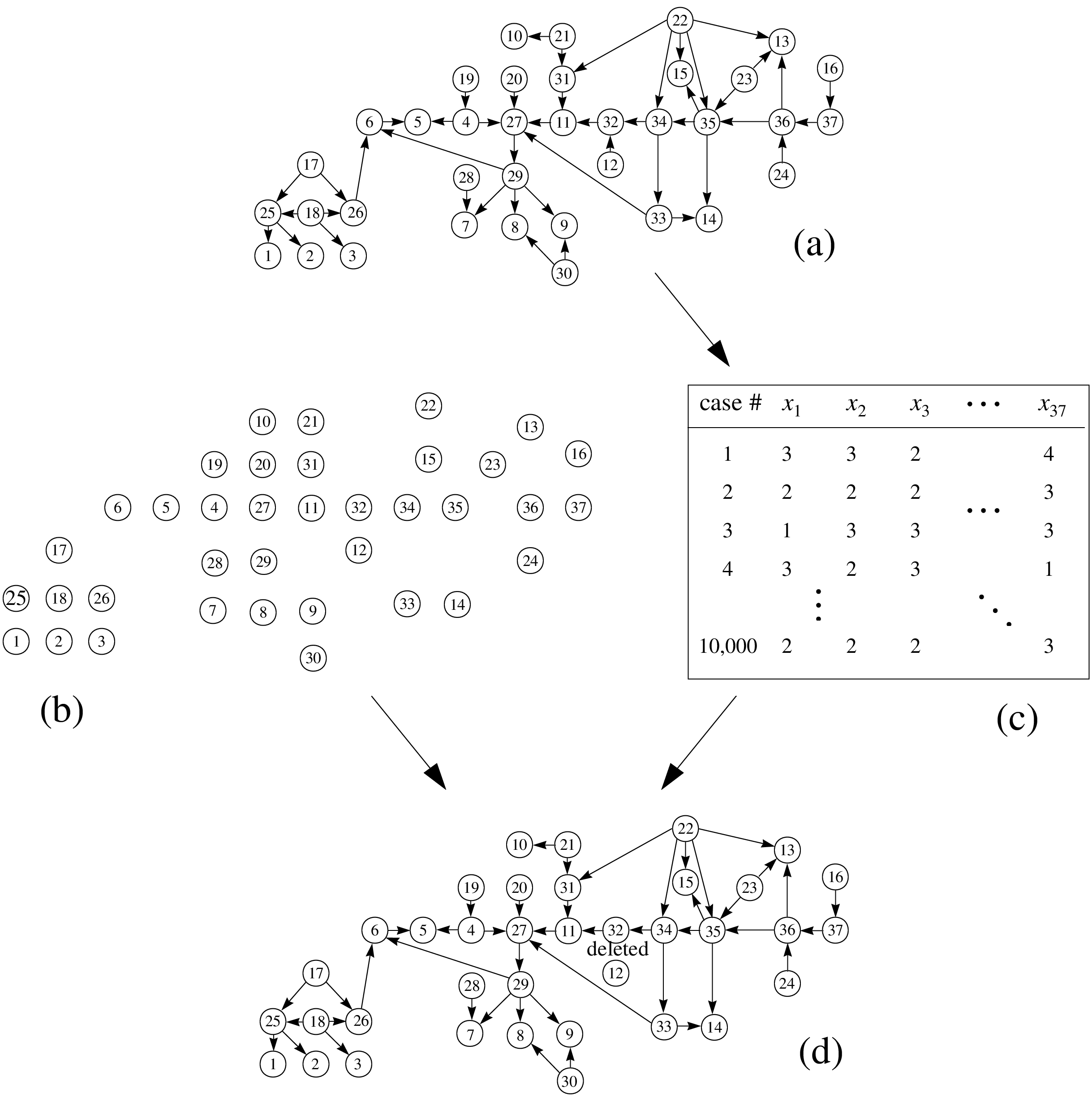
Figure 6: (a) The Alarm network structure. (b) A prior network encoding a user’s beliefs about the Alarm domain. (c) A random sample of size 10,000 generated from the Alarm network. (d) The network learned from the prior network and the random sample. The only difference between the learned and true structure is an arc deletion as noted in (d). Network probabilities are not shown.

13 Bayesian Networks for Supervised Learning

As we discussed in Section 5, the local distribution functions $p(x_{i}|{\bf pa}_{i},\mbox{\boldmath$\theta$}_{i},S^{h})$ are essentially classification/regression models. Therefore, if we are doing supervised learning where the explanatory (input) variables cause the outcome (target) variable and data is complete, then the Bayesian-network and classification/regression approaches are identical.

When data is complete but input/target variables do not have a simple cause/effect relationship, tradeoffs emerge between the Bayesian-network approach and other methods. For example, consider the classification problem in Figure 5. Here, the Bayesian network encodes dependencies between findings and ailments as well as among the findings, whereas another classification model such as a decision tree encodes only the relationships between findings and ailment. Thus, the decision tree may produce more accurate classifications, because it can encode the necessary relationships with fewer parameters. Nonetheless, the use of local criteria for Bayesian-network model selection mitigates this advantage. Furthermore, the Bayesian network provides a more natural representation in which to encode prior knowledge, thus giving this model a possible advantage for sufficiently small sample sizes. Another argument, based on bias–variance analysis, suggests that neither approach will dramatically outperform the other (Friedman, 1996).

Singh and Provan (1995) compare the classification accuracy of Bayesian networks and decision trees using complete data sets from the University of California, Irvine Repository of Machine Learning data sets. Specifically, they compare C4.5 with an algorithm that learns the structure and probabilities of a Bayesian network using a variation of the Bayesian methods we have described. The latter algorithm includes a model-selection phase that discards some input variables. They show that, overall, Bayesian networks and decisions trees have about the same classification error. These results support the argument of Friedman (1996).

When the input variables cause the target variable and data is incomplete, the dependencies between input variables becomes important, as we discussed in the introduction. Bayesian networks provide a natural framework for learning about and encoding these dependencies. Unfortunately, no studies have been done comparing these approaches with other methods for handling missing data.

14 Bayesian Networks for Unsupervised Learning

The techniques described in this paper can be used for unsupervised learning. A simple example is the AutoClass program of Cheeseman and Stutz (1995), which performs data clustering. The idea behind AutoClass is that there is a single hidden (i.e., never observed) variable that causes the observations. This hidden variable is discrete, and its possible states correspond to the underlying classes in the data. Thus, AutoClass can be described by a Bayesian network such as the one in Figure 7. For reasons of computational efficiency, Cheeseman and Stutz (1995) assume that the discrete variables (e.g., $D_{1},D_{2},D_{3}$ in the figure) and user-defined sets of continuous variables (e.g., $\{C_{1},C_{2},C_{3}\}$ and $\{C_{4},C_{5}\}$) are mutually independent given $H$. Given a data set $D$, AutoClass searches over variants of this model (including the number of states of the hidden variable) and selects a variant whose (approximate) posterior probability is a local maximum.

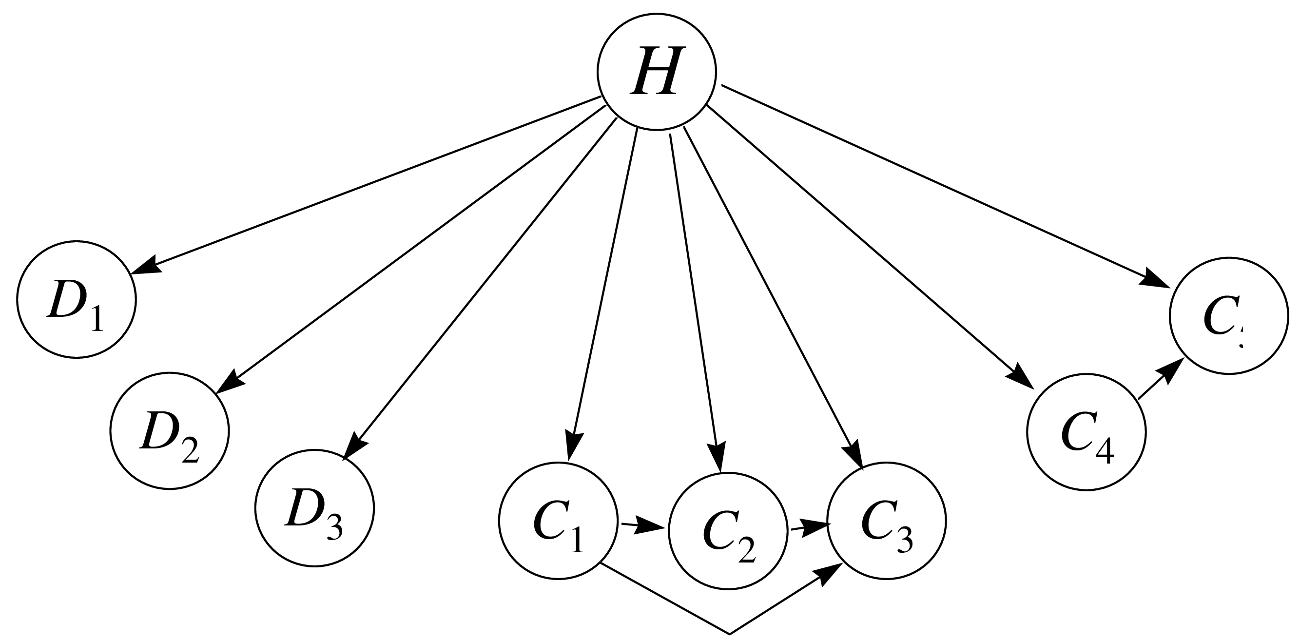
Figure 7: A Bayesian-network structure for AutoClass. The variable $H$ is hidden. Its possible states correspond to the underlying classes in the data.

AutoClass is an example where the user presupposes the existence of a hidden variable. In other situations, we may be unsure about the presence of a hidden variable. In such cases, we can score models with and without hidden variables to reduce our uncertainty. We illustrate this approach on a real-world case study in Section 16. Alternatively, we may have little idea about what hidden variables to model. The search algorithms of Spirtes et al. (1993) provide one method for identifying possible hidden variables in such situations. Martin and VanLehn (1995) suggest another method.

Their approach is based on the observation that if a set of variables are mutually dependent, then a simple explanation is that these variables have a single hidden common cause rendering them mutually independent. Thus, to identify possible hidden variables, we first apply some learning technique to select a model containing no hidden variables. Then, we look for sets of mutually dependent variables in this learned model. For each such set of variables (and combinations thereof), we create a new model containing a hidden variable that renders that set of variables conditionally independent. We then score the new models, possibly finding one better than the original. For example, the model in Figure 8a has two sets of mutually dependent variables. Figure 8b shows another model containing hidden variables suggested by this model.

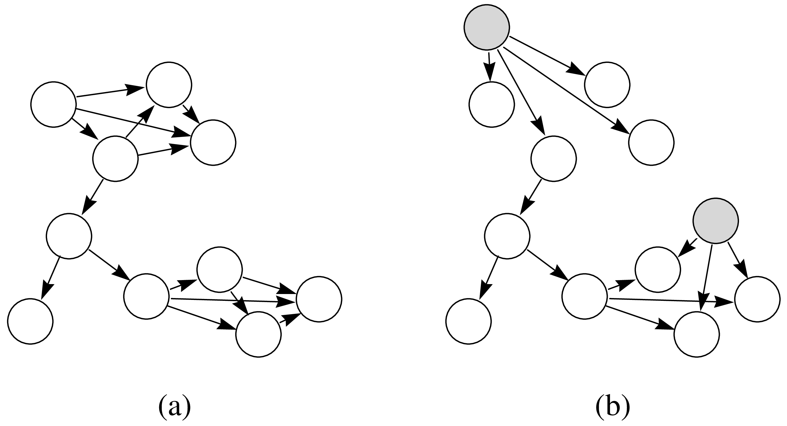
Figure 8: (a) A Bayesian-network structure for observed variables. (b) A Bayesian-network structure with hidden variables (shaded) suggested by the network structure in (a).

15 Learning Causal Relationships

As we have mentioned, the causal semantics of a Bayesian network provide a means by which we can learn causal relationships. In this section, we examine these semantics, and provide a basic discussion on how causal relationships can be learned. We note that these methods are new and controversial. For critical discussions on both sides of the issue, see Spirtes et al. (1993), Pearl (1995), and Humphreys and Freedman (1995).

For purposes of illustration, suppose we are marketing analysts who want to know whether we should increase the placement of a magazine ad to increase sales of a product. If seeing the ad is a cause of busying the product, then we want to show more of it. More generally, causal knowledge is at the heart of understanding what will happen when we intervene. For detailed discussions of the meaning of cause and the close connections between causal knowledge and the consequences of intervention, see Pearl (1995) and Heckerman and Shachter (1995).

How do we learn causal relationships from data? One approach is to actually intervene, and note the consequences. In the classic embodiment of this approach, we perform a randomized experiment. In the ad example, we would (1) select a set of individuals at random, (2) for each individual, show them the ad if and only if a coin flip comes up heads, and (3) note any difference in buying behavior between the two groups. Unfortunately, randomized experiments can be expensive (as in this example), unethical, or difficult to obtain compliance.

Over the last century, many researchers have developed methods for inferring cause and effect. Here, we consider a new approach that makes use of a Bayesian network with causal semantics to infer causal knowledge from observational data alone. The basic idea is to assume a connection between causal and probabilistic relationships in a directed network. More precisely, we say that a directed acyclic graph ${\cal C}$ is a causal graph for variables ${\bf X}$ if the nodes in ${\cal C}$ are in a one-to-one correspondence with ${\bf X}$, and there is an arc from node $X$ to node $Y$ in ${\cal C}$ if and only if $X$ is a direct cause of $Y$. We now assume that if ${\cal C}$ is a causal graph for ${\bf X}$, then ${\cal C}$ is also a Bayesian-network structure for the joint physical probability distribution of ${\bf X}$. This assumption, known as the causal Markov condition, is considered to be quite weak (i.e., quite reasonable) by many philosophers (Spirtes et al., 1993). We can infer causal relationships from observational data by first inferring probabilistic independence relationships as we have described earlier in this tutorial, and then inferring causal relationships using this assumption. As we shall see, we can not always learn causal relationships with this approach. Whether we can, will depend on the probabilistic relationships we find.

To illustrate this approach, let us return to the ad example. Let variables Ad ($A$) and Buy ($B$) represent whether or not an individual has seen the advertisement and has purchased the product, respectively. Assuming these variables are dependent, there are four simple causal explanations: (1) $A$ is a cause of $B$, (2) $B$ is a cause of $A$, (3) there are one or more hidden common causes of $A$ and $B$ (e.g., the person’s gender), and (4) $A$ and $B$ are causes for data selection. This last explanation is an example of selection bias. Condition 4 would occur, for example, if our data set failed to include instances where $A$ and $B$ are false. These four causal explanations for the presence of the arcs are illustrated in Figure 9a. Of course, more complicated explanations—such as the presence of a hidden common cause and selection bias—are possible.

When we have observations only for $A$ and $B$, it is not possible to distinguish among these various causal hypotheses. Suppose, however, that we observe two additional variables: Income ($I$) and Location ($L$), which represent the income and geographic location of the possible purchaser, respectively. Furthermore, suppose we learn (with high probability) the Bayesian network shown in Figure 9b. Given the causal Markov condition, the only causal explanation for the conditional-independence and conditional-dependence relationships encoded in this Bayesian network is that Ad is a cause for Buy. More precisely, none of the other explanations described in the previous paragraph, or combinations thereof, produce the probabilistic relationships encoded in Figure 9b.

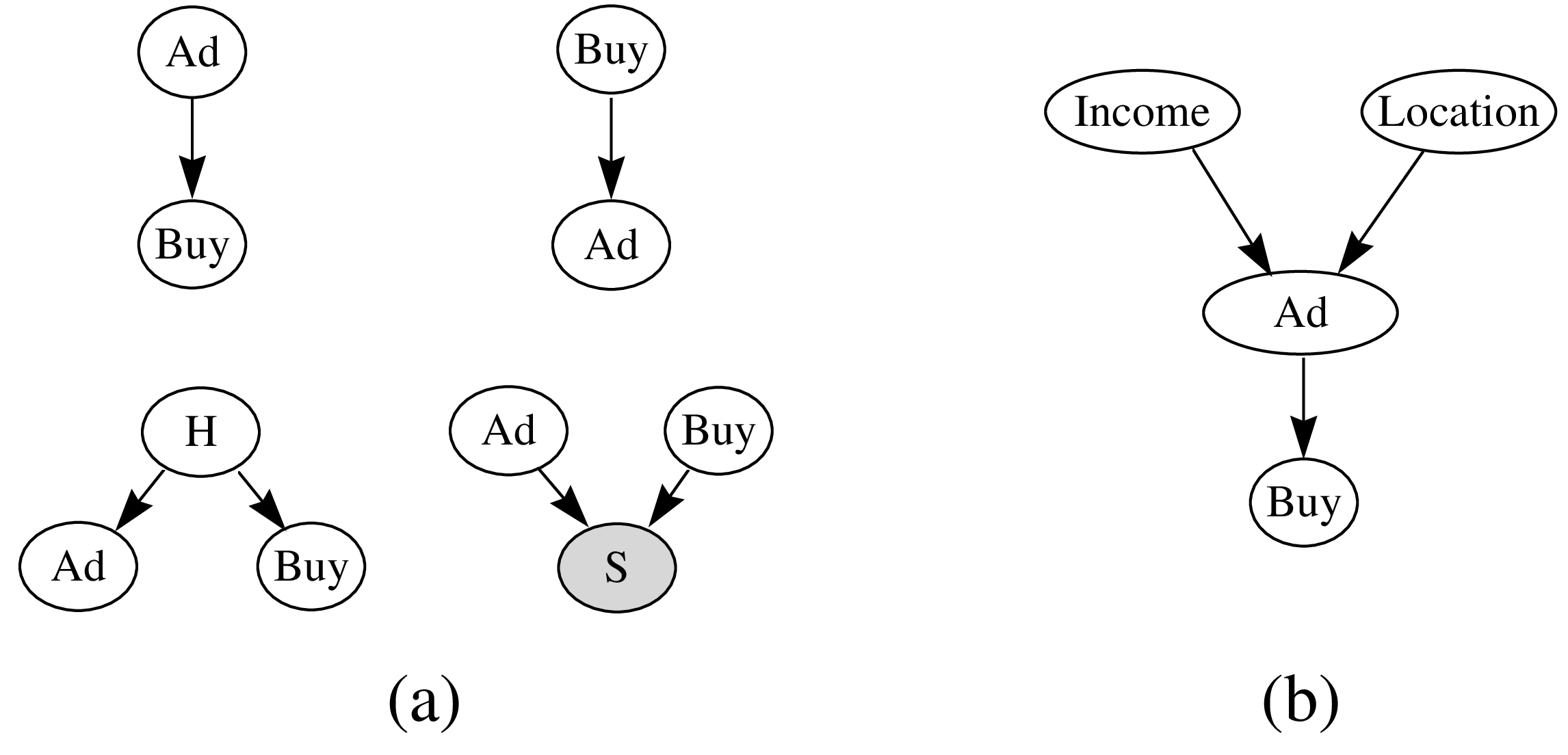
Figure 9: (a) Causal graphs showing four explanations for an observed dependence between Ad and Buy. The node $H$ corresponds to a hidden common cause of Ad and Buy. The shaded node $S$ indicates that the case has been included in the data set. (b) A Bayesian network for which Ad causes Buy is the only causal explanation, given the causal Markov condition.

16 A Case Study: College Plans

Real-world applications of techniques that we have discussed can be found in Madigan and Raftery (1994), Lauritzen et al. (1994), Singh and Provan (1995), and Friedman and Goldszmidt (1996). Here, we consider an application that comes from a study by Sewell and Shah (1968), who investigated factors that influence the intention of high school students to attend college. The data have been analyzed by several groups of statisticians, including Whittaker (1990) and Spirtes et al. (1993), all of whom have used non-Bayesian techniques.

Sewell and Shah (1968) measured the following variables for 10,318 Wisconsin high school seniors: Sex (SEX): male, female; Socioeconomic Status (SES): low, lower middle, upper middle, high; Intelligence Quotient (IQ): low, lower middle, upper middle, high; Parental Encouragement (PE): low, high; and College Plans (CP): yes, no. Our goal here is to understand the (possibly causal) relationships among these variables.

The data are described by the sufficient statistics in Table 2. Each entry denotes the number of cases in which the five variables take on some particular configuration. The first entry corresponds to the configuration SEX$=$male, SES$=$low, IQ$=$low, PE$=$low, and $CP$=yes. The remaining entries correspond to configurations obtained by cycling through the states of each variable such that the last variable (CP) varies most quickly. Thus, for example, the upper (lower) half of the table corresponds to male (female) students.

Table 2: Sufficient statistics for the Sewall and Shah (1968) study.

4	349	13	64	9	207	33	72	12	126	38	54	10	67	49	43
2	232	27	84	7	201	64	95	12	115	93	92	17	79	119	59
8	166	47	91	6	120	74	110	17	92	148	100	6	42	198	73
4	48	39	57	5	47	123	90	9	41	224	65	8	17	414	54
5	454	9	44	5	312	14	47	8	216	20	35	13	96	28	24
11	285	29	61	19	236	47	88	12	164	62	85	15	113	72	50
7	163	36	72	13	193	75	90	12	174	91	100	20	81	142	77
6	50	36	58	5	70	110	76	12	48	230	81	13	49	360	98

Reproduced by permission from the University of Chicago Press. ©1968 by The University of Chicago. All rights reserved.

As a first pass, we analyzed the data assuming there are no hidden variables. To generate priors for network parameters, we used the method described in Section 10.1 with an equivalent sample size of 5 and a prior network where $p({\bf x}|S^{h}_{c})$ is uniform. (The results were not sensitive to the choice of parameter priors. For example, none of the results reported in this section changed qualitatively for equivalent sample sizes ranging from 3 to 40.) We considered all possible structures except those where $SEX$ and/or $SES$ had parents, and/or $CP$ had children. Because the data set was complete, we used Equations 34 and 35 to compute the marginal likelihoods. The two network structures with the highest marginal likelihoods are shown in Figure 10.

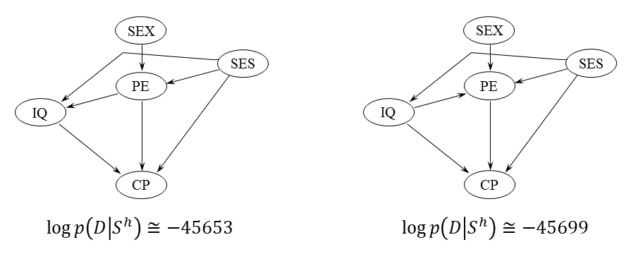
Figure 10: The two network structures without hidden variables with the highest marginal likelihoods.

If we adopt the causal Markov assumption and also assume that there are no hidden variables, then the arcs in both graphs can be interpreted causally. Some results are not surprising—for example the causal influence of socioeconomic status and IQ on college plans. Other results are more interesting. For example, from either graph we conclude that sex influences college plans only indirectly through parental influence. Also, the two graphs differ only by the orientation of the arc between PE and IQ. Either causal relationship is plausible. We note that the second most likely graph was selected by Spirtes et al. (1993), who used a non-Bayesian approach to infer the network.

The most suspicious result is the suggestion that socioeconomic status has a direct influence on IQ. To question this result, we considered new network structures obtained from those in Figure 10 by replacing this direct influence with a hidden variable pointing to both $SES$ and $IQ$, and by inserting a hidden variable between $SES$ and $IQ$. We also considered structures where the hidden variable pointed to $SES$, $IQ$, and $PE$, and none, one, or both of the connections $SES$—$PE$ and $PE$—$IQ$ were removed. For each structure, we varied the number of states of the hidden variable from two to six.

We computed the marginal likelihoods of these structures using the Cheeseman-Stutz (1995) variant of the Laplace approximation. To find the MAP $\tilde{\mbox{\boldmath$\theta$}_{s}}$, we used the EM algorithm, taking the largest local maximum from among 100 runs with different random initializations of $\mbox{\boldmath$\theta$}_{s}$. We then computed more accurate marginal likelihoods for the best networks using annealed importance sampling, a Monte-Carlo technique (Neal, 1998). Among the structures considered, there were two with equal marginal likelihoods, much higher than the marginal likelihoods of the best structures without hidden variables. One is shown in Figure 11. The other has the arc from $H$ to SES reversed. In the model not shown in the figure, SES is a cause of IQ as in the best model with no hidden variables, and $H$ helps to capture the orderings of the states in SES and IQ that are ignored in the multinomial model. In the model shown in the figure, $H$ again helps to capture the ordering of states, but is also a hidden common cause of IQ and SES (e.g.,, parent “quality.”).

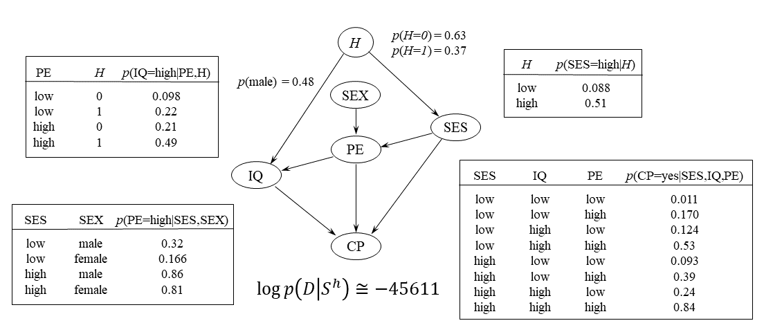
Figure 11: One of the two hidden-variable network structures with the highest marginal likelihood. The other model, which has the same marginal likelihood, has the arc from $H$ to SES reversed. Probabilities shown are MAP values. Some probability distributions are omitted.

In closing, we highlight that model averaging, selective or full, can be applied to Bayesian networks with causal semantics. Applying selective model averaging to the two causal models we have just discussed under the assumption that they are a priori equally likely, the posterior probability that “$H$ causes $SES$” would be 1/2. Furthermore, the posterior probability of $SES$ given that we intervene on $H$ would be the simple average of the probabilities under the two models.

17 Pointers to Literature and Software

Like all tutorials, this one is incomplete. For those readers interested in learning more about graphical models and methods for learning them, we offer the following additional references and pointers to software. Buntine (1996) provides another guide to the literature.

Spirtes et al. (1993) and Pearl (1995) use methods based on large-sample approximations to learn Bayesian networks. In addition, as we have discussed, they describe methods for learning causal relationships from observational data.

In addition to directed models, researchers have explored network structures containing undirected edges as a knowledge representation. These representations are discussed (e.g.) in Lauritzen (1982), Verma and Pearl (1990), Frydenberg (1990), Whittaker (1990), and Richardson (1997). Bayesian methods for learning such models from data are described by Dawid and Lauritzen (1993) and Buntine (1994).

Finally, several research groups have developed software systems for learning graphical models. For example, Scheines et al. (1994) have developed a software program called TETRAD II for learning about cause and effect. Badsberg (1992) and Højsgaard et al. (1994) have built systems that can learn with mixed graphical models using a variety of criteria for model selection. Thomas, Spiegelhalter, and Gilks (1992) have created a system called BUGS that takes a learning problem specified as a Bayesian network and compiles this problem into a Gibbs-sampler computer program.

Notation

$X,Y,Z,\ldots$	Variables or their corresponding nodes in a Bayesian
	network
${\bf X},{\bf Y},{\bf Z},\ldots$	Sets of variables or corresponding sets of nodes
$X=x$	Variable $X$ is in state $x$
${\bf X}={\bf x}$	The set of variables ${\bf X}$ is in configuration ${\bf x}$
${\bf x},{\bf y},{\bf z}$	Typically refer to a complete case, an incomplete
	case, and missing data in a case, respectively
${\bf X}\setminus{\bf Y}$	The variables in $X$ that are not in $Y$
$D$	A data set: a set of cases
$D_{l}$	The first $l-1$ cases in $D$
$p({\bf x}|{\bf y})$	The probability that ${\bf X}={\bf x}$ given ${\bf Y}={\bf y}$
	(also used to describe a probability density,
	probability distribution, and probability density)
${\rm E}_{p(\cdot)}(x)$	The expectation of $x$ with respect to $p(\cdot)$
$S$	A Bayesian network structure (a directed acyclic graph)
${\bf Pa}_{i}$	The variable or node corresponding to the parents
	of node $X_{i}$ in a Bayesian network structure
${\bf pa}_{i}$	A configuration of the variables ${\bf Pa}_{i}$
$r_{i}$	The number of states of discrete variable $X_{i}$
$q_{i}$	The number of configurations of ${\bf Pa}_{i}$
$S_{c}$	A complete network structure
$S^{h}$	The hypothesis corresponding to network structure $S$
$\theta_{ijk}$	The multinomial parameter corresponding to the
	probability $p(X_{i}=x_{i}^{k}|{\bf Pa}_{i}={\bf pa}_{i}^{j})$
$\mbox{\boldmath$\theta$}_{ij}$	$=(\theta_{ij2},\ldots,\theta_{ijr_{i}})$
$\mbox{\boldmath$\theta$}_{i}$	$=(\mbox{\boldmath$\theta$}_{i1},\ldots,\mbox{\boldmath$\theta$}_{iq_{i}})$
$\mbox{\boldmath$\theta$}_{s}$	$=(\mbox{\boldmath$\theta$}_{1},\ldots,\mbox{\boldmath$\theta$}_{n})$
$\alpha$	An equivalent sample size
$\alpha_{ijk}$	The Dirichlet hyperparameter corresponding to $\theta_{ijk}$
$\alpha_{ij}$	$=\sum_{k=1}^{r_{i}}\alpha_{ijk}$
$N_{ijk}$	The number of cases in data set $D$ where $X_{i}=x^{k}_{i}$ and ${\bf Pa}_{i}={\bf pa}_{i}^{j}$
$N_{ij}$	$=\sum_{k=1}^{r_{i}}N_{ijk}$

References

Aliferis, C. and Cooper, G. (1994). An evaluation of an algorithm for inductive learning of Bayesian belief networks using simulated data sets. In Proceedings of Tenth Conference on Uncertainty in Artificial Intelligence, Seattle, WA, pages 8–14. Morgan Kaufmann.

Badsberg, J. (1992). Model search in contingency tables by CoCo. In Dodge, Y. and Whittaker, J., editors, Computational Statistics, pages 251–256. Physica Verlag, Heidelberg.

Becker, S. and LeCun, Y. (1989). Improving the convergence of back-propagation learning with second order methods. In Proceedings of the 1988 Connectionist Models Summer School, pages 29–37. Morgan Kaufmann.

Beinlich, I., Suermondt, H., Chavez, R., and Cooper, G. (1989). The ALARM monitoring system: A case study with two probabilistic inference techniques for belief networks. In Proceedings of the Second European Conference on Artificial Intelligence in Medicine, London, pages 247–256. Springer Verlag, Berlin.

Bernardo, J. (1979). Expected information as expected utility. Annals of Statistics, 7:686–690.

Bernardo, J. and Smith, A. (1994). Bayesian Theory. John Wiley and Sons, New York.

Buntine, W. (1991). Theory refinement on Bayesian networks. In Proceedings of Seventh Conference on Uncertainty in Artificial Intelligence, Los Angeles, CA, pages 52–60. Morgan Kaufmann.

Buntine, W. (1993). Learning classification trees. In Artificial Intelligence Frontiers in Statistics: AI and statistics III. Chapman and Hall, New York.

Buntine, W. (1996). A guide to the literature on learning graphical models. IEEE Transactions on Knowledge and Data Engineering, 8:195–210.

Chaloner, K. and Duncan, G. (1983). Assessment of a beta prior distribution: PM elicitation. The Statistician, 32:174–180.

Cheeseman, P. and Stutz, J. (1995). Bayesian classification (AutoClass): Theory and results. In Fayyad, U., Piatesky-Shapiro, G., Smyth, P., and Uthurusamy, R., editors, Advances in Knowledge Discovery and Data Mining, pages 153–180. AAAI Press, Menlo Park, CA.

Chib, S. (1995). Marginal likelihood from the Gibbs output. Journal of the American Statistical Association, 90:1313–1321.

Chickering, D. (1995). A transformational characterization of equivalent Bayesian network structures. In Proceedings of Eleventh Conference on Uncertainty in Artificial Intelligence, Montreal, QU, pages 87–98. Morgan Kaufmann.

Chickering, D. (1996a). Learning Bayesian Networks from Data. PhD thesis, University of California, Los Angeles, CA.

Chickering, D. (1996b). Learning equivalence classes of Bayesian-network structures. In Proceedings of Twelfth Conference on Uncertainty in Artificial Intelligence, Portland, OR, pages 87–98. Morgan Kaufmann.

Chickering, D., Geiger, D., and Heckerman, D. (1995). Learning Bayesian networks: Search methods and experimental results. In Proceedings of Fifth Conference on Artificial Intelligence and Statistics, Ft. Lauderdale, FL, pages 112–128. Society for Artificial Intelligence in Statistics.

Chickering, D. and Heckerman, D. (Revised November, 1996). Efficient approximations for the marginal likelihood of incomplete data given a Bayesian network. Technical Report MSR-TR-96-08, Microsoft Research, Redmond, WA.

Cooper, G. (1990). Computational complexity of probabilistic inference using Bayesian belief networks (Research note). Artificial Intelligence, 42:393–405.

Cooper, G. and Herskovits, E. (1992). A Bayesian method for the induction of probabilistic networks from data. Machine Learning, 9:309–347.

Cooper, G. and Herskovits, E. (January, 1991). A Bayesian method for the induction of probabilistic networks from data. Technical Report SMI-91-1, Section on Medical Informatics, Stanford University.

Cox, R. (1946). Probability, frequency and reasonable expectation. American Journal of Physics, 14:1–13.

Dagum, P. and Luby, M. (1993). Approximating probabilistic inference in bayesian belief networks is np-hard. Artificial Intelligence, 60:141–153.

D’Ambrosio, B. (1991). Local expression languages for probabilistic dependence. In Proceedings of Seventh Conference on Uncertainty in Artificial Intelligence, Los Angeles, CA, pages 95–102. Morgan Kaufmann.

Darwiche, A. and Provan, G. (1996). Query DAGs: A practical paradigm for implementing belief-network inference. In Proceedings of Twelfth Conference on Uncertainty in Artificial Intelligence, Portland, OR, pages 203–210. Morgan Kaufmann.

Dawid, P. (1984). Statistical theory. The prequential approach (with discussion). Journal of the Royal Statistical Society A, 147:178–292.

Dawid, P. (1992). Applications of a general propagation algorithm for probabilistic expert systmes. Statistics and Computing, 2:25–36.

de Finetti, B. (1970). Theory of Probability. Wiley and Sons, New York.

Dempster, A., Laird, N., and Rubin, D. (1977). Maximum likelihood from incomplete data via the EM algorithm. Journal of the Royal Statistical Society, B 39:1–38.

DiCiccio, T., Kass, R., Raftery, A., and Wasserman, L. (July, 1995). Computing Bayes factors by combining simulation and asymptotic approximations. Technical Report 630, Department of Statistics, Carnegie Mellon University, PA.

Friedman, J. (1995). Introduction to computational learning and statistical prediction. Technical report, Department of Statistics, Stanford University.

Friedman, J. (1996). On bias, variance, 0/1-loss, and the curse of dimensionality. Data Mining and Knowledge Discovery, 1.

Friedman, N. and Goldszmidt, M. (1996). Building classifiers using Bayesian networks. In Proceedings AAAI-96 Thirteenth National Conference on Artificial Intelligence, Portland, OR, pages 1277–1284. AAAI Press, Menlo Park, CA.

Frydenberg, M. (1990). The chain graph Markov property. Scandinavian Journal of Statistics, 17:333–353.

Geiger, D. and Heckerman, D. (Revised February, 1995). A characterization of the Dirichlet distribution applicable to learning Bayesian networks. Technical Report MSR-TR-94-16, Microsoft Research, Redmond, WA.

Geiger, D., Heckerman, D., and Meek, C. (1996). Asymptotic model selection for directed networks with hidden variables. In Proceedings of Twelfth Conference on Uncertainty in Artificial Intelligence, Portland, OR, pages 283–290. Morgan Kaufmann.

Geman, S. and Geman, D. (1984). Stochastic relaxation, Gibbs distributions and the Bayesian restoration of images. IEEE Transactions on Pattern Analysis and Machine Intelligence, 6:721–742.

Gilks, W., Richardson, S., and Spiegelhalter, D. (1996). Markov Chain Monte Carlo in Practice. Chapman and Hall.

Good, I. (1950). Probability and the Weighing of Evidence. Hafners, New York.

Heckerman, D. (1989). A tractable algorithm for diagnosing multiple diseases. In Proceedings of the Fifth Workshop on Uncertainty in Artificial Intelligence, Windsor, ON, pages 174–181. Association for Uncertainty in Artificial Intelligence, Mountain View, CA. Also in Henrion, M., Shachter, R., Kanal, L., and Lemmer, J., editors, Uncertainty in Artificial Intelligence 5, pages 163–171. North-Holland, New York, 1990.

Heckerman, D. (1995). A Bayesian approach for learning causal networks. In Proceedings of Eleventh Conference on Uncertainty in Artificial Intelligence, Montreal, QU, pages 285–295. Morgan Kaufmann.

Heckerman, D. and Geiger, D. (Revised, November, 1996). Likelihoods and priors for Bayesian networks. Technical Report MSR-TR-95-54, Microsoft Research, Redmond, WA.

Heckerman, D., Geiger, D., and Chickering, D. (1995a). Learning Bayesian networks: The combination of knowledge and statistical data. Machine Learning, 20:197–243.

Heckerman, D., Mamdani, A., and Wellman, M. (1995b). Real-world applications of Bayesian networks. Communications of the ACM, 38.

Heckerman, D. and Shachter, R. (1995). Decision-theoretic foundations for causal reasoning. Journal of Artificial Intelligence Research, 3:405–430.

Højsgaard, S., Skjøth, F., and Thiesson, B. (1994). User’s guide to BIOFROST. Technical report, Department of Mathematics and Computer Science, Aalborg, Denmark.

Howard, R. (1970). Decision analysis: Perspectives on inference, decision, and experimentation. Proceedings of the IEEE, 58:632–643.

Howard, R. and Matheson, J. (1981). Influence diagrams. In Howard, R. and Matheson, J., editors, Readings on the Principles and Applications of Decision Analysis, volume II, pages 721–762. Strategic Decisions Group, Menlo Park, CA.

Howard, R. and Matheson, J., editors (1983). The Principles and Applications of Decision Analysis. Strategic Decisions Group, Menlo Park, CA.

Humphreys, P. and Freedman, D. (1996). The grand leap. British Journal for the Philosphy of Science, 47:113–118.

Jaakkola, T. and Jordan, M. (1996). Computing upper and lower bounds on likelihoods in intractable networks. In Proceedings of Twelfth Conference on Uncertainty in Artificial Intelligence, Portland, OR, pages 340–348. Morgan Kaufmann.

Jensen, F. (1996). An Introduction to Bayesian Networks. Springer.

Jensen, F. and Andersen, S. (1990). Approximations in Bayesian belief universes for knowledge based systems. Technical report, Institute of Electronic Systems, Aalborg University, Aalborg, Denmark.

Jensen, F., Lauritzen, S., and Olesen, K. (1990). Bayesian updating in recursive graphical models by local computations. Computational Statisticals Quarterly, 4:269–282.

Kass, R. and Raftery, A. (1995). Bayes factors. Journal of the American Statistical Association, 90:773–795.

Kass, R., Tierney, L., and Kadane, J. (1988). Asymptotics in Bayesian computation. In Bernardo, J., DeGroot, M., Lindley, D., and Smith, A., editors, Bayesian Statistics 3, pages 261–278. Oxford University Press.

Koopman, B. (1936). On distributions admitting a sufficient statistic. Transactions of the American Mathematical Society, 39:399–409.

Korf, R. (1993). Linear-space best-first search. Artificial Intelligence, 62:41–78.

Lauritzen, S. (1982). Lectures on Contingency Tables. University of Aalborg Press, Aalborg, Denmark.

Lauritzen, S. (1992). Propagation of probabilities, means, and variances in mixed graphical association models. Journal of the American Statistical Association, 87:1098–1108.

Lauritzen, S. and Spiegelhalter, D. (1988). Local computations with probabilities on graphical structures and their application to expert systems. J. Royal Statistical Society B, 50:157–224.

Lauritzen, S., Thiesson, B., and Spiegelhalter, D. (1994). Diagnostic systems created by model selection methods: A case study. In Cheeseman, P. and Oldford, R., editors, AI and Statistics IV, volume Lecture Notes in Statistics, 89, pages 143–152. Springer-Verlag, New York.

MacKay, D. (1992a). Bayesian interpolation. Neural Computation, 4:415–447.

MacKay, D. (1992b). A practical Bayesian framework for backpropagation networks. Neural Computation, 4:448–472.

MacKay, D. (1996). Choice of basis for the Laplace approximation. Technical report, Cavendish Laboratory, Cambridge, UK.

Madigan, D., Garvin, J., and Raftery, A. (1995). Eliciting prior information to enhance the predictive performance of Bayesian graphical models. Communications in Statistics: Theory and Methods, 24:2271–2292.

Madigan, D. and Raftery, A. (1994). Model selection and accounting for model uncertainty in graphical models using Occam’s window. Journal of the American Statistical Association, 89:1535–1546.

Madigan, D., Raftery, A., Volinsky, C., and Hoeting, J. (1996). Bayesian model averaging. In Proceedings of the AAAI Workshop on Integrating Multiple Learned Models, Portland, OR.

Madigan, D. and York, J. (1995). Bayesian graphical models for discrete data. International Statistical Review, 63:215–232.

Martin, J. and VanLehn, K. (1995). Discrete factor analysis: Learning hidden variables in bayesian networks. Technical report, Department of Computer Science, University of Pittsburgh, PA. Available at http://bert.cs.pitt.edu/ vanlehn.

Meng, X. and Rubin, D. (1991). Using EM to obtain asymptotic variance-covariance matrices: The SEM algorithm. Journal of the American Statistical Association, 86:899–909.

Neal, R. (1993). Probabilistic inference using Markov chain Monte Carlo methods. Technical Report CRG-TR-93-1, Department of Computer Science, University of Toronto.

Neal, R. (1998). Annealed importance sampling. arXiv:physics/9803008.

Olmsted, S. (1983). On representing and solving decision problems. PhD thesis, Department of Engineering-Economic Systems, Stanford University.

Pearl, J. (1986). Fusion, propagation, and structuring in belief networks. Artificial Intelligence, 29:241–288.

Pearl, J. (1995). Causal diagrams for empirical research. Biometrika, 82:669–710.

Pearl, J. and Verma, T. (1991). A theory of inferred causation. In Allen, J., Fikes, R., and Sandewall, E., editors, Knowledge Representation and Reasoning: Proceedings of the Second International Conference, pages 441–452. Morgan Kaufmann, New York.

Pitman, E. (1936). Sufficient statistics and intrinsic accuracy. Proceedings of the Cambridge Philosophy Society, 32:567–579.

Raftery, A. (1995). Bayesian model selection in social research. In Marsden, P., editor, Sociological Methodology. Blackwells, Cambridge, MA.

Raftery, A. (1996). Hypothesis testing and model selection, chapter 10. Chapman and Hall.

Ramamurthi, K. and Agogino, A. (1988). Real time expert system for fault tolerant supervisory control. In Tipnis, V. and Patton, E., editors, Computers in Engineering, pages 333–339. American Society of Mechanical Engineers, Corte Madera, CA.

Ramsey, F. (1931). Truth and probability. In Braithwaite, R., editor, The Foundations of Mathematics and other Logical Essays. Humanities Press, London. Reprinted in Kyburg and Smokler, 1964.

Richardson, T. (1997). Extensions of undirected and acyclic, directed graphical models. In Proceedings of Sixth Conference on Artificial Intelligence and Statistics, Ft. Lauderdale, FL, pages 407–419. Society for Artificial Intelligence in Statistics.

Rissanen, J. (1987). Stochastic complexity (with discussion). Journal of the Royal Statistical Society, Series B, 49:223–239 and 253–265.

Robins, J. (1986). A new approach to causal interence in mortality studies with sustained exposure results. Mathematical Modelling, 7:1393–1512.

Rubin, D. (1978). Bayesian inference for causal effects: The role of randomization. Annals of Statistics, 6:34–58.

Russell, S., Binder, J., Koller, D., and Kanazawa, K. (1995). Local learning in probabilistic networks with hidden variables. In Proceedings of the Fourteenth International Joint Conference on Artificial Intelligence, Montreal, QU, pages 1146–1152. Morgan Kaufmann, San Mateo, CA.

Saul, L., Jaakkola, T., and Jordan, M. (1996). Mean field theory for sigmoid belief networks. Journal of Artificial Intelligence Research, 4:61–76.

Savage, L. (1954). The Foundations of Statistics. Dover, New York.

Schervish, M. (1995). Theory of Statistics. Springer-Verlag.

Schwarz, G. (1978). Estimating the dimension of a model. Annals of Statistics, 6:461–464.

Sewell, W. and Shah, V. (1968). Social class, parental encouragement, and educational aspirations. American Journal of Sociology, 73:559–572.

Shachter, R. (1988). Probabilistic inference and influence diagrams. Operations Research, 36:589–604.

Shachter, R., Andersen, S., and Poh, K. (1990). Directed reduction algorithms and decomposable graphs. In Proceedings of the Sixth Conference on Uncertainty in Artificial Intelligence, Boston, MA, pages 237–244. Association for Uncertainty in Artificial Intelligence, Mountain View, CA.

Shachter, R. and Kenley, C. (1989). Gaussian influence diagrams. Management Science, 35:527–550.

Silverman, B. (1986). Density Estimation for Statistics and Data Analysis. Chapman and Hall, New York.

Singh, M. and Provan, G. (November, 1995). Efficient learning of selective Bayesian network classifiers. Technical Report MS-CIS-95-36, Computer and Information Science Department, University of Pennsylvania, Philadelphia, PA.

Spetzler, C. and Stael von Holstein, C. (1975). Probability encoding in decision analysis. Management Science, 22:340–358.

Spiegelhalter, D., Dawid, A., Lauritzen, S., and Cowell, R. (1993). Bayesian analysis in expert systems. Statistical Science, 8:219–282.

Spiegelhalter, D. and Lauritzen, S. (1990). Sequential updating of conditional probabilities on directed graphical structures. Networks, 20:579–605.

Spirtes, P., Glymour, C., and Scheines, R. (1993). Causation, Prediction, and Search. Springer-Verlag, New York.

Spirtes, P. and Meek, C. (1995). Learning Bayesian networks with discrete variables from data. In Proceedings of First International Conference on Knowledge Discovery and Data Mining, Montreal, QU, pages 294–299. Morgan Kaufmann.

Suermondt, H. and Cooper, G. (1991). A combination of exact algorithms for inference on Bayesian belief networks. International Journal of Approximate Reasoning, 5:521–542.

Thiesson, B. (1995a). Accelerated quantification of Bayesian networks with incomplete data. In Proceedings of First International Conference on Knowledge Discovery and Data Mining, Montreal, QU, pages 306–311. Morgan Kaufmann.

Thiesson, B. (1995b). Score and information for recursive exponential models with incomplete data. Technical report, Institute of Electronic Systems, Aalborg University, Aalborg, Denmark.

Thomas, A., Spiegelhalter, D., and Gilks, W. (1992). Bugs: A program to perform Bayesian inference using Gibbs sampling. In Bernardo, J., Berger, J., Dawid, A., and Smith, A., editors, Bayesian Statistics 4, pages 837–842. Oxford University Press.

Tukey, J. (1977). Exploratory Data Analysis. Addison–Wesley.

Tversky, A. and Kahneman, D. (1974). Judgment under uncertainty: Heuristics and biases. Science, 185:1124–1131.

Verma, T. and Pearl, J. (1990). Equivalence and synthesis of causal models. In Proceedings of Sixth Conference on Uncertainty in Artificial Intelligence, Boston, MA, pages 220–227. Morgan Kaufmann.

Whittaker, J. (1990). Graphical Models in Applied Multivariate Statistics. John Wiley and Sons.

Winkler, R. (1967). The assessment of prior distributions in Bayesian analysis. American Statistical Association Journal, 62:776–800.