Non-Stationary Ruijsenaars Functions for $\kappa=t^{-1/N}$

Non-Stationary Ruijsenaars Functions for $\boldsymbol{\kappa=t^{-1/N}}$
and Intertwining Operators of Ding–Iohara–Miki
Algebra

Masayuki FUKUDA ^†, Yusuke OHKUBO ^‡ and Jun’ichi SHIRAISHI ^‡

M. Fukuda, Y. Ohkubo and J. Shiraishi

^† Department of Physics, Faculty of Science, The University of Tokyo,
^† Hongo 7-3-1, Bunkyo-ku, Tokyo 113-0033 Japan phy.m.fukuda@gmail.com

^‡ Graduate School of Mathematical Sciences, The University of Tokyo,
^‡ Komaba 3-8-1, Meguro-ku, Tokyo 153-8914 Japan yusuke.ohkubo.math@gmail.com, shiraish@ms.u-tokyo.ac.jp

Received April 23, 2020, in final form November 01, 2020; Published online November 18, 2020

We construct the non-stationary Ruijsenaars functions (affine analogue of the Macdonald functions) in the special case $\kappa=t^{-1/N}$, using the intertwining operators of the Ding–Iohara–Miki algebra (DIM algebra) associated with $N$-fold Fock tensor spaces. By the $S$-duality of the intertwiners, another expression is obtained for the non-stationary Ruijsenaars functions with $\kappa=t^{-1/N}$, which can be regarded as a natural elliptic lift of the asymptotic Macdonald functions to the multivariate elliptic hypergeometric series. We also investigate some properties of the vertex operator of the DIM algebra appearing in the present algebraic framework; an integral operator which commutes with the elliptic Ruijsenaars operator, and the degeneration of the vertex operators to the Virasoro primary fields in the conformal limit $q\rightarrow 1$.

Macdonald function; Rujisenaars function; Ding–Iohara–Miki algebra

33D52; 81R10

1 Introduction

The non-stationary Ruijsenaars function $f^{\widehat{\mathfrak{gl}}_{N}}(\boldsymbol{x},p|\boldsymbol{s},\kappa|q,t)$ introduced by one of the authors in [44] is by definition given in the form of the Nekrasov partition function,

$$f^{\widehat{\mathfrak{gl}}_{N}}(\boldsymbol{x},p|\boldsymbol{s},\kappa|q,t)$$

$$\qquad{}=\sum_{\lambda^{(1)},\ldots,\lambda^{(N)}\in{\mathsf{P}}}\prod_{i,j=1}^{N}{\mathsf{N}^{(j-i|N)}_{\lambda^{(i)},\lambda^{(j)}}(ts_{j}/s_{i}|q,\kappa)\over\mathsf{N}^{(j-i|N)}_{\lambda^{(i)},\lambda^{(j)}}(s_{j}/s_{i}|q,\kappa)}\prod_{\beta=1}^{N}\prod_{\alpha\geq 1}(px_{\alpha+\beta}/tx_{\alpha+\beta-1})^{\lambda^{(\beta)}_{\alpha}}.$$ (1.1)

Here $\boldsymbol{x}=(x_{1},\ldots,x_{N})$, $\boldsymbol{s}=(s_{1},\ldots,s_{N})$, and $N\in\mathbb{Z}_{\geq 1}$. As for the detail, see Definition 3.21. Our goal in the present paper is to establish the transformation formula stated in Theorem 3.30 below for the non-stationary Ruijsenaars function $f^{\widehat{\mathfrak{gl}}_{N}}$ in the special case $\kappa=t^{-1/N}$, by using the $S$-duality of the intertwining operators of the Ding–Iohara–Miki (DIM) algebra.

Define the elliptic shifted product $\Theta(a;q,p)_{n}$ as the ratio of the Ruijsenaars elliptic gamma function $\Gamma(a;q,p)$ by

$$\Theta(a;q,p)_{n}:=\frac{\Gamma(q^{n}a;q,p)}{\Gamma(a;q,p)},\qquad\Gamma(a;q,p):=\frac{(qp/a;q,p)_{\infty}}{(a;q,p)_{\infty}}.$$ (1.2)

[Definition 3.24]Define $f^{\mathrm{ellip}}_{N}(\boldsymbol{x};\boldsymbol{s}|q,t,p)\in\mathbb{Q}(q,t,\boldsymbol{s})[[p,x_{2}/x_{1},\ldots,x_{N}/x_{N-1}]]$ by

$$f^{\mathrm{ellip}}_{N}(\boldsymbol{x};\boldsymbol{s}|q,t,p)=\sum_{\theta\in\mathsf{M}_{N}}c^{\mathrm{ellip}}_{N}(\theta;\boldsymbol{s}|q,q/t,p)\prod_{1\leq i<j\leq N}(x_{j}/x_{i})^{\theta_{ij}},$$

where $\mathsf{M}_{N}=\{(\theta_{ij})_{1\leq i,j\leq N}\,|\,\theta_{ij}\in\mathbb{Z}_{\geq 0},\,\theta_{kl}=0\mbox{ if }k\geq l\}$ is the set of $N\times N$ strictly upper triangular matrices with nonnegative integer entries, and

$$c^{\mathrm{ellip}}_{N}(\theta;\boldsymbol{s}|q,t,p)=\prod_{k=2}^{N}\prod_{1\leq i<j\leq k}\dfrac{\Theta(q^{\sum_{a>k}(\theta_{ia}-\theta_{ja})}ts_{j}/s_{i};q,p)_{\theta_{ik}}}{\Theta(q^{\sum_{a>k}(\theta_{ia}-\theta_{ja})}qs_{j}/s_{i};q,p)_{\theta_{ik}}}$$

$$\hphantom{c^{\mathrm{ellip}}_{N}(\theta;\boldsymbol{s}|q,t,p)=}{}\times\prod_{k=2}^{N}\prod_{1\leq i\leq j<k}\dfrac{\Theta(q^{-\theta_{jk}+\sum_{a>k}(\theta_{ia}-\theta_{ja})}qs_{j}/ts_{i};q,p)_{\theta_{ik}}}{\Theta(q^{-\theta_{jk}+\sum_{a>k}(\theta_{ia}-\theta_{ja})}s_{j}/s_{i};q,p)_{\theta_{ik}}}.$$

[Theorem 3.30]As a formal series in $p$, $s_{i+1}/s_{i}$, $x_{i+1}/x_{i}$ $(i=1,\ldots,N-1)$ and $px_{1}/x_{N}$, we have

$$f^{\widehat{\mathfrak{gl}}_{N}}\big{(}\boldsymbol{x}{}^{\prime},p^{{1}/{N}}|\boldsymbol{s}^{\prime},t^{-{1}/{N}}|q,t\big{)}=\mathfrak{C}\times f^{\mathrm{ellip}}_{N}(\boldsymbol{s};\boldsymbol{x}|q,t,p),$$ (1.3)

where

$$\mathfrak{C}:=\left(\frac{(pq/t;q,p)_{\infty}}{(p;p)_{\infty}(pt;q,p)_{\infty}}\right)^{N}\prod_{1\leq i<j\leq N}\frac{\Gamma(tx_{j}/x_{i};q,p)}{\Gamma(qx_{j}/x_{i};q,p)}\prod_{1\leq i<j\leq N}\frac{(ts_{j}/s_{i};q)_{\infty}}{(qs_{j}/s_{i};q)_{\infty}},$$

$$\boldsymbol{s}^{\prime}=(s^{\prime}_{1},\ldots,s^{\prime}_{N}),\qquad s^{\prime}_{k}=t^{{k}/{N}}s_{k},\qquad\boldsymbol{x}^{\prime}=(x^{\prime}_{1},\ldots,x^{\prime}_{N}),\qquad x^{\prime}_{k}=p^{-{k}/{N}}x_{k}.$$

The shifts of $\boldsymbol{s}^{\prime}$ and $\boldsymbol{x}^{\prime}$ correspond to the ones used in the limit $p\rightarrow 0$ (Fact A.8). These shifts appear naturally in the construction by $p$-trace of vertex operators that we will explain later.

Contrary to the case $N\geq 2$, the case $N=1$ seems somewhat special from the point of view of our vertex operator approach, and the parameter $\kappa$ can be treated as an arbitrary constant. As a result, we have the following summation formula, which has been already proved by [12, 35]. [Theorem 3.41]We have

$$\exp\left(\sum\frac{1}{n}\frac{(1-q^{n}\kappa^{n})(1-\kappa^{n}/t^{n})\kappa^{-n}p^{n}}{(1-q^{n})(1-t^{-n})(1-p^{n})}\right)$$

$$\qquad{}=\sum_{\lambda\in\mathsf{P}}(p/\kappa)^{|\lambda|}\frac{\prod_{1\leq i\leq j}(\kappa q^{-\lambda_{i}+\lambda_{j+1}}t^{i-j};q)_{\lambda_{j}-\lambda_{j+1}}(\kappa q^{\lambda_{i}-\lambda_{j}}t^{-i+j+1};q)_{\lambda_{j}-\lambda_{j+1}}}{\prod_{1\leq i\leq j}(q^{-\lambda_{i}+\lambda_{j+1}}t^{i-j};q)_{\lambda_{j}-\lambda_{j+1}}(q^{\lambda_{i}-\lambda_{j}}t^{-i+j+1};q)_{\lambda_{j}-\lambda_{j+1}}}.$$ (1.4)

Remark that setting $\kappa=t^{-1}$ in (1.4), we recover (1.3) for $N=1$. To prove Theorem 3.30 and Theorem 3.41, we use the technique of the topological vertex operator. This consists of the DIM algebra, the trivalent vertex operators, and the web diagrams encoding the structure of the Fock tensor spaces which the DIM algebra is acting on.

To fix a good starting point, we need to recall some facts about the asymptotically free eigenfunctions $f^{\mathfrak{gl}_{N}}(\boldsymbol{x},\boldsymbol{s}|q,t)$ for the Macdonald $q$-difference operator. See [11, 31, 42] and Appendix A as to the basic facts.

[Definition 3.12] Define the formal series $f^{\mathfrak{gl}_{N}}(\boldsymbol{x};\boldsymbol{s}|q,t)\in\mathbb{Q}(q,t,\boldsymbol{s})[[x_{2}/x_{1},\ldots,\allowbreak x_{N}/x_{N-1}]]$ by

$$f^{\mathfrak{gl}_{N}}(\boldsymbol{x};\boldsymbol{s}|q,t)=\sum_{\theta\in\mathsf{M}_{N}}c_{N}(\theta;\boldsymbol{s}|q,t)\prod_{1\leq i<j\leq N}(x_{j}/x_{i})^{\theta_{ij}},$$

where the coefficient $c_{N}(\theta;\boldsymbol{s}|q,t)$ is defined by

$$c_{N}(\theta;\boldsymbol{s}|q,t)=\prod_{k=2}^{N}\prod_{1\leq i<j\leq k}\dfrac{(q^{\sum_{a>k}(\theta_{ia}-\theta_{ja})}ts_{j}/s_{i};q)_{\theta_{ik}}}{(q^{\sum_{a>k}(\theta_{ia}-\theta_{ja})}qs_{j}/s_{i};q)_{\theta_{ik}}}$$

$$\hphantom{c_{N}(\theta;\boldsymbol{s}|q,t)=}{}\times\prod_{k=2}^{N}\prod_{1\leq i\leq j<k}\dfrac{(q^{-\theta_{jk}+\sum_{a>k}(\theta_{ia}-\theta_{ja})}qs_{j}/ts_{i};q)_{\theta_{ik}}}{(q^{-\theta_{jk}+\sum_{a>k}(\theta_{ia}-\theta_{ja})}s_{j}/s_{i};q)_{\theta_{ik}}}.$$

The Macdonald $q$-difference operator is derived from the trigonometric case of the Ruijsenaars models [36] which is given as a relativistic generalization of the Calogero–Morser–Sutherland systems [34]. Explicit eigenfunctions of the Macdonald $q$-difference operator (trigonometric Ruijsenaars operator) have been studied, and they are called Macdonald symmetric polynomials [27]. Whereas the Macdonald polynomials are parametrized by partitions, the function $f^{\mathfrak{gl}_{N}}$ in Definition 3.12 is series with parameters $s_{i}$. Specialization of $s_{i}$’s gives us ordinary Macdonald polynomials associated with partitions. Note that the $f^{\mathfrak{gl}_{N}}$ also enjoys the eigenvalue equation (Fact A.2), the analytic property (Fact A.7), the bispectral duality (Fact A.4), and the Poincaré duality (Fact A.5). Ruijsenaars introduced not only the trigonometric integral model but also the general elliptic version [36]. In the elliptic case, however, it seems we still lack a fundamental understanding of the properties of eigenfunctions. See [20, 38, 39], for example. One of our motivations for studying the non-stationary Ruijsenaars functions (1.1) comes from the strong hope that the non-stationary function might have much simpler combinatorial or analytic properties than the original elliptic stationary Ruijsenaars functions. Some of the observations given in [44] read: (1) it is conjectured that the non-stationary Ruijsenaars functions $f^{\widehat{\mathfrak{gl}}_{N}}$ with a suitable normalization procedure give explicit solutions to the elliptic Ruijsenaars models in the very (essentially) singular limit $\kappa\rightarrow 1$. (2) $f^{\widehat{\mathfrak{gl}}_{N}}$ reduce to the asymptotically free Macdonald eigenfunctions $f^{\mathfrak{gl}_{N}}$ in the limit $p\rightarrow 0$. (3) We have the bispectral duality and the Poincaré duality for $f^{\widehat{\mathfrak{gl}}_{N}}$.

We have a “web diagrammatic description” of the combinatorial structure of $f^{\mathfrak{gl}_{N}}$ (Definition 3.12), based on the DIM algebra. In other words, the $f^{\mathfrak{gl}_{N}}$ has an interpretation as a certain Nekrasov partition function associated with the web diagram. See [21, 30, 46].

The DIM algebra has two kinds of intertwining operators, $\Phi\colon\mathcal{F}^{(0,1)}\otimes\mathcal{F}^{(1,0)}\rightarrow\mathcal{F}^{(1,1)}$ and $\Phi^{*}\colon\mathcal{F}^{(1,1)}\rightarrow\mathcal{F}^{(1,0)}\otimes\mathcal{F}^{(0,1)}$ among the triple of Fock spaces, introduced in [6]. As for the definition of the modules $\mathcal{F}^{(1,M)}$, $\mathcal{F}^{(0,1)}$ and the intertwiners, see Facts 2.5, 2.4, and 2.6. By using physics terminology, we refer to the modules $\mathcal{F}^{(0,1)}$ as the preferred directions. The matrix elements of these intertwiners are identical to the refined topological vertex. We express the composition $\Phi^{*}\circ\Phi$ by the cross diagram in Fig. 1, left.

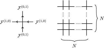
Figure 1: $\Phi^{*}\circ\Phi$ and $f^{\mathfrak{gl}_{N}}$.

Compose these operators reticulately as in Fig. 1, right. Specialize spectral parameters in a certain manner. Attach empty diagrams to all the external edges. Then we have the Macdonald function $f^{\mathfrak{gl}_{N}}$ as thus constructed matrix element (see Fact 3.13).

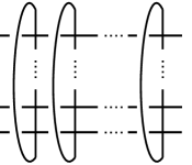
Figure 2: The cylindric web diagram for the non-stationary Ruijsenaars functions $f^{\widehat{\mathfrak{gl}}_{N}}$.

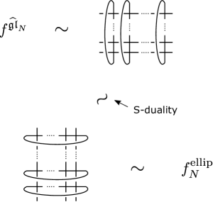
Figure 3: The sketch of the proof.

Suppose we consider the trace in the preferred or vertical direction, instead of the matrix element as above. See Fig. 2 below. We will prove that the $p$-trace associated with the web on a cylinder gives us the non-stationary Ruijsenaars function $f^{\widehat{\mathfrak{gl}}_{N}}$ for the special parameter $\kappa=t^{-1/N}$ for $N\geq 2$, and for generic $\kappa$ for $N=1$.

Thanks to the $S$-duality, we can flip the diagram, obtaining the picture as in Fig. 3. Finally, the trace in the horizontal direction can be calculated by the standard technique, thereby giving the elliptic lift $f^{\mathrm{ellip}}_{N}$ of the asymptotically free eigenfunction $f^{\mathfrak{gl}_{N}}$ for the Macdonald $q$-difference operator. In Section 3 are given our proofs of Theorems 3.30 and 3.41 which go along this idea.

Some explanations are in order, concerning the physical background and recent related works on the non-stationary systems, including the non-stationary Heun, Lamé, and elliptic Calogero–Sutherland equations. These non-stationary equations have been extensively studied based on the perturbative approach by Atai and Langmann in [3]. Recently in [4], they obtained an integral formula for the eigenfunctions for the non-stationary elliptic Calogero–Sutherland equation for some special choices of the parameter in the “time derivative” term, using the kernel function technique.

Note that no explicit equations have been obtained for the non-stationary Ruijsenaars function $f^{\widehat{\mathfrak{gl}}_{N}}$ unfortunately. So the authors have been lead to use the representation theories of the DIM algebra, to bypass the troublesome situation without any eigenvalue equations or associated kernel functions. One may find, nevertheless, the resulting formula in Theorem 3.30 can be regarded as a $q$-difference analogue of Atai and Langmann’s integral formula in [4], suggesting the existence of $q$-analogue of the kernel functions.

The function $f^{\widehat{\mathfrak{gl}}_{N}}$ is by definition a series which can be regarded as a Jackson integral, whereas the eigenfunction in [4] is given in terms of a contour integral. The functions $f^{\widehat{\mathfrak{gl}}_{N}}$ is parametrized by the continuous parameters $s_{i}$, while Atai and Langmann’s integral formula contains a partition as a set of discrete parameters. The integral formula in [4] works not only for $\kappa^{\prime}=g$ but also for $\kappa^{\prime}=kg$ ($k=2,3,\ldots$), where $\kappa^{\prime}$ and $g$ are parameters corresponding to $\kappa$ and $t$ as $\kappa={\rm e}^{\kappa^{\prime}\hbar}$, $t={\rm e}^{g\hbar}$. It is an interesting problem to find a similar construction of the non-stationary Ruijsenaars functions for $\kappa=t^{-k/N}$ ($k=2,3,\ldots$).

In this occasion, we address some other related problems in the representation theory of the DIM algebra. First, we derive an integral operator $I(s_{1}/s_{0},\ldots,s_{N}/s_{0})$ introduced in [40, 41, 43] from the intertwining operators of the DIM algebra. As for the definition of $I(s_{1}/s_{0},\ldots,s_{N}/s_{0})$, see Definition 4.6. In [40, 41, 43], it was conjectured that the integral operator $I(s_{1}/s_{0},\ldots,s_{N}/s_{0})$ commutes with Macdonald’s difference operator. A proof has been given in [31]. We provide yet another perspective based on the vertex operator. We also discuss the elliptic analogue of the integral operator. Our elliptic integral operator can be constructed by taking the loop of intertwining operators. It commutes with the Ruijsenaars operator.

Secondly, we study the conformal limit $q\rightarrow 1$ of the $2N$-valent intertwining operator $\mathcal{V}(z)$, which is a main object in the authors’ previous paper [21], restricting ourselves to the simplest nontrivial case $N=2$. The operator $\mathcal{V}(z)$ is defined by the relations with the $q$-$W_{N}$ algebra, the $q$-Vir algebra for $N=2$. We will derive the well-known relation of the Virasoro primary fields from those defining relations in the limit $q\rightarrow 1$. In [21], a formula for the matrix elements of $\mathcal{V}(z)$ with respect to generalized Macdonald functions (Fact 2.21) are proved. The result Theorem 5.25 and the matrix elements formula for $\mathcal{V}(z)$ prove that the generalized Macdonald functions are reduced to Alba, Fateev Litvinov and Tarnopolskii’s basis [1]. Hence, the matrix element formula for $\mathcal{V}(z)$ provides us with another proof of the 4-dimensional AGT correspondence [2].

This paper is organized as follows. Basic facts with respect to the intertwining operators of the DIM algebra are summarized in Section 2. In Section 3, we reproduce the non-stationary Ruijsenaars functions from the intertwiners on the cylindric web diagrams. We also prove Theorem 3.30 by using the $S$-duality. In Section 4, we derive the integral operator $I(s_{1}/s_{0},\ldots,s_{N}/s_{0})$ and prove the commutativity with the Macdonald $q$-difference operator. The elliptic extension of the integral operator is also discussed. We take the conformal limit $q\rightarrow 1$ in Section 5. In Appendix A, some facts with respect to Macdonald functions $f^{\mathfrak{gl}_{N}}$ are explained. In Appendix B, we describe the construction of the non-stationary Ruijsenaars functions from the affine screening operators in the case of general $\kappa$. In Appendix C are given some straightforward but cumbersome details needed for our proofs.

Notation

We use the following standard symbols for the $q$-shifted factorials, the theta functions and the elliptic gamma functions [22]:

$$(a;q)_{\infty}:=\prod_{n=1}^{\infty}\big{(}1-q^{n-1}a\big{)},\qquad(a;q)_{m}:=\frac{(a;q)_{\infty}}{(aq^{m};q)_{\infty}},$$

$$\theta_{q}(a):=(a;q)_{\infty}\big{(}qa^{-1};q\big{)}_{\infty},$$

$$(a;q,p)_{\infty}:=\prod_{n,m=1}^{\infty}\big{(}1-q^{n-1}p^{m-1}a\big{)},\qquad\Gamma(a;q,p):=\frac{(qp/a;q,p)_{\infty}}{(a;q,p)_{\infty}}.$$

For integers $n\leq m$, we use the following symbols for the tensor product and the ordered products

$$\bigotimes_{n\leq i\leq m}^{\curvearrowright}A_{i}:=A_{n}\otimes A_{n+1}\otimes\cdots\otimes A_{m},$$

$$\prod_{n\leq i\leq m}^{\curvearrowright}A_{i}:=A_{n}\times A_{n+1}\times\cdots\times A_{m},$$

$$\prod_{n\leq i\leq m}^{\curvearrowleft}A_{i}:=A_{m}\times A_{m-1}\times\cdots\times A_{n}.$$

A partition $\lambda=(\lambda_{1},\lambda_{2},\ldots)$ is a sequence of nonnegative integers such that $\lambda_{1}\geq\lambda_{2}\geq\cdots$ with finitely many nonzero elements $\lambda_{j}$. The empty diagram is denoted by $\emptyset=(0,0,\ldots)$. $\mathsf{P}$ denotes the set of all partitions. For $\lambda\in\mathsf{P}$, we write $|\lambda|=\sum_{i\geq 1}\lambda_{i}$ and $\ell(\lambda)=\#\{i\,|\,\lambda_{i}\neq 0\}$. The conjugate partition of $\lambda$ is denoted by $\lambda^{\prime}$. If $\lambda_{i}\leq\mu_{i}$ for all $i$, we write $\lambda\subset\mu$. For an $N$-tuple of partitions $\boldsymbol{\lambda}=\big{(}\lambda^{(1)},\lambda^{(2)},\ldots,\lambda^{(N)}\big{)}\in\mathsf{P}^{N}$, write $|\boldsymbol{\lambda}|=\big{|}\lambda^{(1)}\big{|}+\cdots+\big{|}\lambda^{(N)}\big{|}$. For a pair of positive integers $(i,j)\in\mathbb{Z}^{2}_{>0}$, the arm length $a_{\lambda}(i,j)$ and the leg length $\ell_{\lambda}(i,j)$ are defined by

$$a_{\lambda}(i,j)=\lambda_{i}-j,\qquad\ell_{\lambda}(i,j)=\lambda^{\prime}_{j}-i.$$

2 DIM algebra, intertwiners, and Mukadé operators

We briefly recall the definition of the Ding–Iohara–Miki (DIM) algebra [13, 28], its intertwining operators and the $S$-duality formula for the intertwining operators. Let $q$ and $t$ be generic complex parameters with $|q|$, $|t^{-1}|<1$.

Definition 2.1.

The DIM algebra, which we denote by $\mathcal{U}=\mathcal{U}_{q,t}$, is a unital associative algebra generated by the currents $x^{\pm}(z)=\sum_{n\in\mathbb{Z}}x^{\pm}_{n}z^{-n}$, $\psi^{\pm}(z)=\sum_{\pm n\in\mathbb{Z}_{\geq 0}}\psi^{\pm}_{n}z^{-n}$ and the central elements $c^{\pm 1/2}$. The defining relations are

$$\psi^{+}(z)x^{\pm}(w)=g\big{(}c^{\mp 1/2}w/z\big{)}^{\mp 1}x^{\pm}(w)\psi^{+}(z),$$

$$\psi^{-}(z)x^{\pm}(w)=g\big{(}c^{\mp 1/2}z/w\big{)}^{\pm 1}x^{\pm}(w)\psi^{-}(z),$$

$$\psi^{\pm}(z)\psi^{\pm}(w)=\psi^{\pm}(w)\psi^{\pm}(z),\qquad\psi^{+}(z)\psi^{-}(w)=\dfrac{g\big{(}c^{+1}w/z\big{)}}{g\big{(}c^{-1}w/z\big{)}}\psi^{-}(w)\psi^{+}(z),$$

$$\big{[}x^{+}(z),x^{-}(w)\big{]}=\dfrac{(1-q)(1-1/t)}{1-q/t}\big{(}\delta\big{(}c^{-1}z/w\big{)}\psi^{+}\big{(}c^{1/2}w\big{)}-\delta(cz/w)\psi^{-}\big{(}c^{-1/2}w\big{)}\big{)},$$

$$G^{\mp}(z/w)x^{\pm}(z)x^{\pm}(w)=G^{\pm}(z/w)x^{\pm}(w)x^{\pm}(z),$$

where

$$g(z)=\dfrac{G^{+}(z)}{G^{-}(z)},\qquad G^{\pm}(z)=\big{(}1-q^{\pm 1}z\big{)}\big{(}1-t^{\mp 1}z\big{)}\big{(}1-q^{\mp 1}t^{\pm 1}z\big{)},\qquad\delta(z)=\sum_{n\in\mathbb{Z}}z^{n}.$$

Fact 2.2 ([13]).

The Drinfeld coproduct

$$\Delta\big{(}c^{\pm 1/2}\big{)}=c^{\pm 1/2}\otimes c^{\pm 1/2},$$

$$\Delta\big{(}x^{+}(z)\big{)}=x^{+}(z)\otimes 1+\psi^{-}\big{(}c_{(1)}^{1/2}z\big{)}\otimes x^{+}(c_{(1)}z),$$

$$\Delta\big{(}x^{-}(z)\big{)}=x^{-}(c_{(2)}z)\otimes\psi^{+}\big{(}c_{(2)}^{1/2}z\big{)}+1\otimes x^{-}(z),$$

$$\Delta\big{(}\psi^{\pm}(z)\big{)}=\psi^{\pm}\big{(}c_{(2)}^{\pm 1/2}z\big{)}\otimes\psi^{\pm}\big{(}c_{(1)}^{\mp 1/2}z\big{)}$$

gives rise to a bialgebra structure. Further, $\mathcal{U}$ has a Hopf algebra structure. We omit the counit and the antipode.

A $\mathcal{U}$-module is called of level-$(n,m)$ if the central elements act as $c=(t/q)^{n/2}$ and $(\psi^{+}_{0}/\psi^{-}_{0})^{1/2}\allowbreak=(q/t)^{m/2}$. In this paper, we use two kinds of $\mathcal{U}$-modules. The first one is a free field representation with the following boson. Let $\mathcal{H}$ be the Heisenberg algebra generated by $\{a_{n}\,|\,n\in\mathbb{Z}\}$ with the commutation relation

$$[a_{n},a_{m}]=n\frac{1-q^{|n|}}{1-t^{|n|}}\delta_{n+m,0}.$$

Let $\ket{0}$ and $\bra{0}$ be the highest weight vectors defined by $a_{n}\ket{0}=0$ ($n\geq 0$) and $\bra{0}a_{n}=0$ ($n\leq 0$), respectively. Denote by $\mathcal{F}$ (resp. $\mathcal{F}^{*}$) the Fock space generated from the highest weight vector $\ket{0}$ (resp. $\bra{0}$). The bilinear form $\mathcal{F}^{*}\otimes\mathcal{F}\rightarrow\mathbb{C}$ is defined by setting $\braket{0}{0}=1$.

Definition 2.3.

Define the vertex operators $\eta(z)$, $\xi(z)$ and $\varphi^{\pm}(z)\in\mathrm{End}(\mathcal{F})\big{[}\big{[}z^{\pm 1}\big{]}\big{]}$ by

$$\eta(z)=\exp\bigg{(}\sum_{n=1}^{\infty}\dfrac{1-t^{-n}}{n}a_{-n}z^{n}\bigg{)}\exp\bigg{(}{-}\sum_{n=1}^{\infty}\dfrac{1-t^{n}}{n}a_{n}z^{-n}\bigg{)},$$

$$\xi(z)=\exp\bigg{(}{-}\sum_{n=1}^{\infty}\dfrac{1-t^{-n}}{n}q^{-n/2}t^{n/2}a_{-n}z^{n}\bigg{)}\exp\bigg{(}\sum_{n=1}^{\infty}\dfrac{1-t^{n}}{n}q^{-n/2}t^{n/2}a_{n}z^{-n}\bigg{)},$$

$$\varphi^{+}(z)=\exp\bigg{(}{-}\sum_{n=1}^{\infty}\dfrac{1-t^{n}}{n}\big{(}1-t^{n}q^{-n}\big{)}q^{n/4}t^{-n/4}a_{n}z^{-n}\bigg{)},$$

$$\varphi^{-}(z)=\exp\bigg{(}\sum_{n=1}^{\infty}\dfrac{1-t^{-n}}{n}\big{(}1-t^{n}q^{-n}\big{)}q^{n/4}t^{-n/4}a_{-n}z^{n}\bigg{)}.$$

Fact 2.4 ([15]).

Let $u$ be an indeterminate and $M$ be an integer. The algebra homomorphism $\rho_{u}\colon\mathcal{U}\rightarrow\mathrm{End}(\mathcal{F})$ defined by

$$c^{1/2}\mapsto(t/q)^{1/4},\qquad x^{+}(z)\mapsto uz^{-M}q^{-M/2}t^{M/2}\eta(z),\qquad x^{-}(z)\mapsto u^{-1}z^{M}q^{M/2}t^{-M/2}\xi(z),$$

$$\psi^{+}(z)\mapsto q^{M/2}t^{-M/2}\varphi^{+}(z),\qquad\psi^{-}(z)\mapsto q^{-M/2}t^{M/2}\varphi^{-}(z)$$

endows $\mathcal{F}$ with the level $(1,M)$-module structure.

We denote by $\mathcal{F}^{(1,M)}_{u}$ the Fock space endowed with the level $(1,M)$-module structure. The dual space $\mathcal{F}^{*}$ can also be endowed with the right $\mathcal{U}$-module structure through $\rho_{u}$. Then it is denoted by $\mathcal{F}^{(1,M)*}_{u}$. The $\rho_{u}$ is called the horizontal representation.

Next, we consider the level $(0,1)$-module. Let $\mathcal{F}^{(0,1)}$ be the vector space spanned by the vectors $\ket{\lambda}$ with $\lambda\in\mathsf{P}$. Define $(\bra{\lambda}\,|\,\lambda\in\mathsf{P})$ to be the dual basis such that $\braket{\lambda}{\mu}=\delta_{\lambda,\mu}$.

Fact 2.5 ([14, 19]).

Let $u$ be an indeterminate. The following action gives the level $(0,1)$-module structure to $\mathcal{F}^{(0,1)}$:

$$c^{1/2}\ket{\lambda}=\ket{\lambda},$$

$$x^{+}(z)\ket{\lambda}=\sum_{i=1}^{\ell(\lambda)+1}A^{+}_{\lambda,i}\delta\big{(}q^{\lambda_{i}}t^{-i+1}u/z\big{)}\ket{\lambda+{\bf 1}_{i}},$$

$$x^{-}(z)\ket{\lambda}=q^{1/2}t^{-1/2}\sum_{i=1}^{\ell(\lambda)}A^{-}_{\lambda,i}\delta\big{(}q^{\lambda_{i}-1}t^{-i+1}u/z\big{)}\ket{\lambda-{\bf 1}_{i}},$$

$$\psi^{+}(z)\ket{\lambda}=q^{1/2}t^{-1/2}B^{+}_{\lambda}(u/z)\ket{\lambda},$$

$$\psi^{-}(z)\ket{\lambda}=q^{-1/2}t^{1/2}B^{-}_{\lambda}(z/u)\ket{\lambda}.$$

Here, $A^{\pm}_{\lambda,i}\in\mathbb{Q}(q,t)$ and $B^{+}_{\lambda}(z)\in\mathbb{Q}(q,t)[[z]]$ are defined by

$$A^{+}_{\lambda,i}=(1-t)\prod_{j=1}^{i-1}{\big{(}1-q^{\lambda_{i}-\lambda_{j}}t^{-i+j+1}\big{)}\big{(}1-q^{\lambda_{i}-\lambda_{j}+1}t^{-i+j-1}\big{)}\over\big{(}1-q^{\lambda_{i}-\lambda_{j}}t^{-i+j}\big{)}\big{(}1-q^{\lambda_{i}-\lambda_{j}+1}t^{-i+j}\big{)}},$$

$$A^{-}_{\lambda,i}=(1-t^{-1}){1-q^{\lambda_{i+1}-\lambda_{i}}\over 1-q^{\lambda_{i+1}-\lambda_{i}+1}t^{-1}}\prod_{j=i+1}^{\infty}{\big{(}1-q^{\lambda_{j}-\lambda_{i}+1}t^{-j+i-1}\big{)}\big{(}1-q^{\lambda_{j+1}-\lambda_{i}}t^{-j+i}\big{)}\over\big{(}1-q^{\lambda_{j+1}-\lambda_{i}+1}t^{-j+i-1}\big{)}\big{(}1-q^{\lambda_{j}-\lambda_{i}}t^{-j+i}\big{)}},$$

$$B^{+}_{\lambda}(z)={1-q^{\lambda_{1}-1}tz\over 1-q^{\lambda_{1}}z}\prod_{i=1}^{\infty}{\big{(}1-q^{\lambda_{i}}t^{-i}z\big{)}\big{(}1-q^{\lambda_{i+1}-1}t^{-i+1}z\big{)}\over\big{(}1-q^{\lambda_{i+1}}t^{-i}z\big{)}\big{(}1-q^{\lambda_{i}-1}t^{-i+1}z\big{)}},$$

$$B^{-}_{\lambda}(z)={1-q^{-\lambda_{1}+1}t^{-1}z\over 1-q^{-\lambda_{1}}z}\prod_{i=1}^{\infty}{\big{(}1-q^{-\lambda_{i}}t^{i}z\big{)}\big{(}1-q^{-\lambda_{i+1}+1}t^{i-1}z\big{)}\over\big{(}1-q^{-\lambda_{i+1}}t^{i}z\big{)}\big{(}1-q^{-\lambda_{i}+1}t^{i-1}z\big{)}}.$$

We denote this module by $\mathcal{F}^{(0,1)}_{u}$. This is called the vertical representation or the preferred direction. By using the two representations, the trivalent intertwiners $\Phi$, $\Phi^{\ast}$ of the DIM algebra were introduced in [6].

Fact 2.6 ([6]).

Let $M$ be an integer. If $w=-vu$, there exists a unique linear operator

$$\Phi\left[(1,M+1),w\atop(0,1),v;(1,M),u\right]\colon\ \mathcal{F}^{(0,1)}_{v}\otimes\mathcal{F}^{(1,M)}_{u}\longrightarrow\mathcal{F}^{(1,M+1)}_{w}$$

such that $\bra{0}\Phi(\ket{\emptyset}\otimes\ket{0})=1$ and

$$a\Phi=\Phi\Delta(a)\qquad(\forall\,a\in\mathcal{U}).$$

Similarly, there exists a unique linear operator

$$\Phi^{*}\left[(1,M),u;(0,1),v\atop(1,M+1),-vu\right]\colon\ \mathcal{F}^{(1,M+1)}_{-uv}\longrightarrow\mathcal{F}^{(1,M)}_{u}\otimes\mathcal{F}^{(0,1)}_{v}$$

such that $(\bra{0}\otimes\bra{\emptyset})\Phi^{*}\ket{0}=1$ and

$$\Delta(a)\Phi^{*}=\Phi^{*}a\qquad(\forall\,a\in\mathcal{U}).$$

It is known that these intertwining operators can be realized as follows.

Definition 2.7.

For a partition $\lambda$, define the $\lambda$-component $\Phi_{\lambda}$ of $\Phi$

$$\Phi_{\lambda}\left[(1,M+1),-uv\atop(0,1),v;(1,M),u\right]\colon\ \mathcal{F}^{(1,M)}_{u}\rightarrow\mathcal{F}^{(1,M+1)}_{-uv}$$

by

$$\Phi_{\lambda}(\alpha)=\Phi(\ket{\lambda}\otimes\alpha)\qquad\big{(}\forall\,\alpha\in\mathcal{F}^{(1,M)}_{u}\big{)}.$$

Similarly, define the $\lambda$-component $\Phi^{\ast}_{\lambda}$ of $\Phi^{\ast}$

$$\Phi^{*}_{\lambda}\left[(1,M),u;(0,1),v\atop(1,M+1),-vu\right]\colon\ \mathcal{F}^{(1,M+1)}_{-uv}\rightarrow\mathcal{F}^{(1,M)}_{u}$$

by

$$\Phi^{*}(\alpha)=\sum_{\lambda\in\mathsf{P}}\Phi^{*}_{\lambda}(\alpha)\otimes\ket{\lambda}\qquad\big{(}\forall\,\alpha\in\mathcal{F}^{(1,M+1)}_{-uv}\big{)}.$$

Notation 2.8.

For $\lambda\in\mathsf{P}$, set

$$n(\lambda)=\sum_{i\geq 1}(i-1)\lambda_{i},\qquad f_{\lambda}=(-1)^{|\lambda|}q^{n(\lambda^{\prime})+|\lambda|/2}t^{-n(\lambda)-|\lambda|/2},$$

$$c_{\lambda}:=\prod_{(i,j)\in\lambda}\big{(}1-q^{a_{\lambda}(i,j)}t^{\ell_{\lambda}(i,j)+1}\big{)},\qquad c^{\prime}_{\lambda}:=\prod_{(i,j)\in\lambda}\big{(}1-q^{a_{\lambda}(i,j)+1}t^{\ell_{\lambda}(i,j)}\big{)}.$$

Fact 2.9 ([6]).

$\Phi_{\lambda}$ is of the form

$$\Phi_{\lambda}\left[(1,M+1),-vu\atop(0,1),v;(1,M),u\right]=\hat{t}(\lambda,u,v,M)\widehat{\Phi}_{\lambda}(v),$$

where

$$\hat{t}(\lambda,u,v,M)=(-vu)^{|\lambda|}(-v)^{-(M+1)|\lambda|}f_{\lambda}^{-M-1}q^{n(\lambda^{\prime})}/c_{\lambda},$$

$$\widehat{\Phi}_{\lambda}(v)={:}\Phi_{\emptyset}(v)\eta_{\lambda}(v){:},$$

$$\Phi_{\emptyset}(v)=\exp\bigg{(}{-}\sum_{n=1}^{\infty}\dfrac{1}{n}\dfrac{1}{1-q^{n}}a_{-n}v^{n}\bigg{)}\exp\bigg{(}{-}\sum_{n=1}^{\infty}\dfrac{1}{n}\dfrac{q^{n}}{1-q^{n}}a_{n}v^{-n}\bigg{)},$$

$$\eta_{\lambda}(v)={:}\prod_{i=1}^{\ell(\lambda)}\prod_{j=1}^{\lambda_{i}}\eta(q^{j-1}t^{-i+1}v){:}.$$

The symbol ${:}\cdots{:}$ means the usual normal ordering product. Similarly, $\Phi^{*}_{\lambda}$ is of the form

$$\Phi^{*}_{\lambda}\left[(1,M),v;(0,1),u\atop(1,M+1),-vu\right]=\hat{t}^{*}(\lambda,u,v,M)\widehat{\Phi}^{*}_{\lambda}(u),$$

where

$$\hat{t}^{*}(\lambda,u,v,M)=(q^{-1}v)^{-|\lambda|}(-u)^{M|\lambda|}f_{\lambda}^{M}q^{n(\lambda^{\prime})}/c^{\prime}_{\lambda},$$

$$\widehat{\Phi}^{*}_{\lambda}(u)={:}\Phi^{*}_{\emptyset}(u)\xi_{\lambda}(u){:},$$

$$\Phi^{*}_{\emptyset}(u)=\exp\bigg{(}\sum_{n=1}^{\infty}\dfrac{1}{n}\dfrac{1}{1-q^{n}}q^{-n/2}t^{n/2}a_{-n}u^{n}\bigg{)}\exp\bigg{(}\sum_{n=1}^{\infty}\dfrac{1}{n}\dfrac{q^{n}}{1-q^{n}}q^{-n/2}t^{n/2}a_{n}u^{-n}\bigg{)},$$

$$\xi_{\lambda}(u)={:}\prod_{i=1}^{\ell(\lambda)}\prod_{j=1}^{\lambda_{i}}\xi(q^{j-1}t^{-i+1}u){:}.$$

Figure 4: The trivalent intertwining operators. Left: $\Phi$, Right: $\Phi^{*}$. Note that the diagrams in this papar are flipped horizontally for the ones in [21].

Throughout the paper, the case $M=0$ is concerned. The intertwining operators $\Phi$ and $\Phi^{*}$ are expressed as the trivalent diagrams in Fig. 4. It is known that their matrix elements coincide with the Iqbal, Kozcaz and Vafa’s or Awata and Kanno’s refined topological vertecies [6, 8, 24], and the vertical representation corresponds to the preferred direction. We prepare the formula for the normal ordering of the intertwiners, in which the Nekrasov factor appears.

Definition 2.10.

Define the Nekrasov factor to be

$$N_{\lambda\mu}(u):=\prod_{(i,j)\in\lambda}\big{(}1-uq^{-a_{\mu}(i,j)-1}t^{-\ell_{\lambda}(i,j)}\big{)}\prod_{(i,j)\in\mu}\big{(}1-uq^{a_{\lambda}(i,j)}t^{\ell_{\mu}(i,j)+1}\big{)}$$

$$\hphantom{N_{\lambda\mu}(u):\!}{}=\prod_{(i,j)\in\lambda}\big{(}1-uq^{a_{\lambda}(i,j)}t^{\ell_{\mu}(i,j)+1}\big{)}\prod_{(i,j)\in\mu}\big{(}1-uq^{-a_{\mu}(i,j)-1}t^{-\ell_{\lambda}(i,j)}\big{)}.$$

Fact 2.11 ([6]).

Put $\gamma=(t/q)^{1/2}$. We have

$$\Phi_{\lambda^{(i)}}(v_{i})\Phi^{*}_{\mu^{(j)}}(u_{j})=\mathcal{G}(u_{j}/\gamma v_{i})^{-1}N_{\mu^{(j)}\lambda^{(i)}}(u_{j}/\gamma v_{i}){:}\Phi_{\lambda^{(i)}}(v_{i})\Phi^{*}_{\mu^{(j)}}(u_{j}){:},$$

$$\Phi^{*}_{\mu^{(j)}}(u_{j})\Phi_{\lambda^{(i)}}(v_{i})=\mathcal{G}(v_{i}/\gamma u_{j})^{-1}N_{\lambda^{(i)}\mu^{(j)}}(v_{i}/\gamma u_{j}){:}\Phi^{*}_{\mu^{(j)}}(u_{j})\Phi_{\lambda^{(i)}}(v_{i}){:},$$

$$\Phi_{\lambda^{(i)}}(v_{i})\Phi_{\lambda^{(j)}}(v_{j})=\frac{\mathcal{G}(v_{j}/\gamma^{2}v_{i})}{N_{\lambda^{(j)}\lambda^{(i)}}(v_{j}/\gamma^{2}v_{i})}{:}\Phi_{\lambda^{(i)}}(v_{i})\Phi_{\lambda^{(j)}}(v_{j}){:},$$

$$\Phi^{*}_{\mu^{(i)}}(u_{i})\Phi^{*}_{\mu^{(j)}}(u_{j})=\frac{\mathcal{G}(u_{j}/u_{i})}{N_{\mu^{(j)}\mu^{(i)}}(u_{j}/u_{i})}{:}\Phi^{*}_{\mu^{(i)}}(u_{i})\Phi^{*}_{\mu^{(j)}}(u_{j}){:},$$

where $\mathcal{G}(z)=\prod_{i,j=0}^{\infty}\big{(}1-zq^{i}t^{-j}\big{)}=\big{(}z;q,t^{-1}\big{)}_{\infty}$.

Furthermore, we introduce the following operators for convenience, which is expressed by the cross diagram in Fig. 5.

Figure 5: The operator $\Phi^{\mathrm{cr}}$.

Definition 2.12.

Define

$$\Phi^{\mathrm{cr}}\left[v;{us/v\atop s};u\right]=\dfrac{\Phi^{*}\left[\displaystyle(1,0),v;(0,1),us/v\atop\displaystyle(1,1),-us\right]\circ\Phi\left[\displaystyle(1,1),-us\atop\displaystyle(0,1),s;(1,0),u\right]}{\bra{0}\Phi^{*}_{\emptyset}\left[\displaystyle(1,0),v;(0,1),us/v\atop\displaystyle(1,1),-us\right]\Phi_{\emptyset}\left[\displaystyle(1,1),-us\atop\displaystyle(0,1),s;(1,0),u\right]\ket{0}},$$

$$\Phi^{\mathrm{cr}}\left[v;{us/v,\mu\atop s,\lambda};u\right]=\dfrac{\Phi^{*}_{\mu}\left[\displaystyle(1,0),v;(0,1),us/v\atop\displaystyle(1,1),-us\right]\Phi_{\lambda}\left[\displaystyle(1,1),-us\atop\displaystyle(0,1),s;(1,0),u\right]}{\bra{0}\Phi^{*}_{\emptyset}\left[\displaystyle(1,0),v;(0,1),us/v\atop\displaystyle(1,1),-us\right]\Phi_{\emptyset}\left[\displaystyle(1,1),-us\atop\displaystyle(0,1),s;(1,0),u\right]\ket{0}}.$$

Let $N\in\mathbb{Z}_{\geq 1}$. The main objects in the previous paper [21] are the following $2N$-valent intertwiners, which we called the Mukadé operators after the shape of diagrams obtained by connecting the trivalent diagrams. (“Mukade” means centipedes in Japanese. See Fig. 6.)

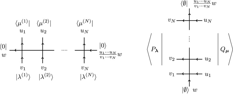
Figure 6: The $S$-duality formula.

Definition 2.13.

Take the composition

$$\bigg{(}\bigotimes_{1\leq i\leq N}^{\curvearrowright}\mathcal{F}^{(0,1)}_{v_{i}}\bigg{)}\otimes\mathcal{F}^{(1,0)}_{w^{\prime}}\xrightarrow{{\rm id}\otimes\cdots\otimes{\rm id}\otimes\Phi^{\mathrm{cr}}}\bigg{(}\bigotimes_{1\leq i\leq N-1}^{\curvearrowright}\mathcal{F}^{(0,1)}_{v_{i}}\bigg{)}\otimes\mathcal{F}^{(1,0)}_{\frac{v_{N}}{u_{N}}w^{\prime}}\otimes\mathcal{F}^{(0,1)}_{u_{N}}$$

$$\hphantom{\bigg{(}\bigotimes_{1\leq i\leq N}^{\curvearrowright}\mathcal{F}^{(0,1)}_{v_{i}}\bigg{)}\otimes}\xrightarrow{{\rm id}\otimes\cdots\otimes{\rm id}\otimes\Phi^{\mathrm{cr}}\otimes{\rm id}}\cdots\xrightarrow{\Phi^{\mathrm{cr}}{\rm id}\otimes\cdots\otimes{\rm id}}\mathcal{F}^{(1,0)}_{w}\otimes\bigotimes_{1\leq i\leq N}^{\curvearrowright}\mathcal{F}^{(0,1)}_{u_{i}}.$$ (2.1)

Here $w^{\prime}=\frac{u_{1}\cdots u_{N}}{v_{1}\cdots v_{N}}w$. Define the operator

$$T^{H}(\boldsymbol{u},\boldsymbol{v},w)\colon\ \bigotimes_{1\leq i\leq N}^{\curvearrowright}\mathcal{F}^{(0,1)}_{v_{i}}\rightarrow\bigotimes_{1\leq i\leq N}^{\curvearrowright}\mathcal{F}^{(0,1)}_{u_{i}}$$

as the vacuum expectation value $\bra{0}\cdots\ket{0}$ of the operator $(\ref{eq: comp. for PhiH})$ with respect to the level $(1,0)$ representation. Furthermore, we define the normalized operator

$$\mathcal{T}^{H}(\boldsymbol{u},\boldsymbol{v},w)=\frac{T^{H}(\boldsymbol{u},\boldsymbol{v},w)}{\bra{\boldsymbol{\emptyset}}T^{H}(\boldsymbol{u},\boldsymbol{v},w)\ket{\boldsymbol{\emptyset}}}.$$

Here, we have set $\ket{\boldsymbol{\emptyset}}=\ket{\emptyset}\otimes\cdots\otimes\ket{\emptyset}$.

Definition 2.14.

Define the operators

$$T^{V}(\boldsymbol{u},\boldsymbol{v},w),\mathcal{T}^{V}(\boldsymbol{u},\boldsymbol{v},w)\colon\ \bigotimes_{1\leq i\leq N}^{\curvearrowright}\mathcal{F}^{(1,0)}_{u_{i}}\rightarrow\bigotimes_{1\leq i\leq N}^{\curvearrowright}\mathcal{F}^{(1,0)}_{v_{i}}$$

by

$$T^{V}(\boldsymbol{u},\boldsymbol{v},w)=\sum_{\mu^{(1)},\ldots,\mu^{(N-1)}\in\mathsf{P}}\bigotimes^{\curvearrowright}_{1\leq k\leq N}\Phi^{\mathrm{cr}}\left[v_{k};{\frac{u_{k}}{v_{k}}w_{k},\mu^{(k)}\atop w_{k},\mu^{(k-1)}};u_{k}\right]\qquad\big{(}\mu^{(0)}=\mu^{(N)}=\emptyset\big{)},$$

$$\mathcal{T}^{V}(\boldsymbol{u},\boldsymbol{v},w)=\frac{T^{V}(\boldsymbol{u},\boldsymbol{v},w)}{\bra{\boldsymbol{0}}T^{V}(\boldsymbol{u},\boldsymbol{v},w)\ket{\boldsymbol{0}}}.$$

Here, $w_{k}=\frac{u_{1}\cdots u_{k-1}}{v_{1}\cdots v_{k-1}}w$.

We prepare some notations to treat the $N$-fold Fock tensor spaces.

Notation 2.15.

We write

$$\mathcal{F}_{\boldsymbol{u}}^{(N,0)}=\bigotimes_{1\leq i\leq N}^{\curvearrowright}\mathcal{F}^{(1,0)}_{u_{i}},\qquad\mathcal{F}_{\boldsymbol{u}}^{(N,0)*}=\bigotimes_{1\leq i\leq N}^{\curvearrowright}\mathcal{F}^{(1,0)*}_{u_{i}},$$

$$\mathcal{F}_{\boldsymbol{u}}^{(0,N)}=\bigotimes_{1\leq i\leq N}^{\curvearrowright}\mathcal{F}^{(0,1)}_{u_{i}}\qquad(\boldsymbol{u}=(u_{1},\ldots,u_{N})),$$

$$a^{(i)}_{n}=\overbrace{1\otimes\cdots\otimes 1}^{i-1}\otimes a_{n}\otimes\overbrace{1\otimes\dots\otimes 1}^{N-i}.$$

For $\boldsymbol{\lambda}=\big{(}\lambda^{(1)},\ldots,\lambda^{(N)}\big{)}\in\mathsf{P}^{N}$, set

$$\ket{\boldsymbol{\lambda}}=\bigotimes_{1\leq i\leq N}^{\curvearrowright}\ket{\lambda^{(i)}},\qquad\bra{\boldsymbol{\lambda}}=\bigotimes_{1\leq i\leq N}^{\curvearrowright}\bra{\lambda^{(i)}},$$

$$\ket{a_{\boldsymbol{\lambda}}}=a^{(1)}_{-\lambda^{(1)}_{1}}a^{(1)}_{-\lambda^{(1)}_{2}}\cdots a^{(2)}_{-\lambda^{(2)}_{1}}a^{(2)}_{-\lambda^{(2)}_{2}}\cdots a^{(N)}_{-\lambda^{(N)}_{1}}a^{(N)}_{-\lambda^{(N)}_{2}}\ket{\boldsymbol{0}},$$

$$\bra{a_{\boldsymbol{\lambda}}}=\bra{\boldsymbol{0}}\cdots a^{(N)}_{\lambda^{(N)}_{2}}a^{(N)}_{\lambda^{(N)}_{1}}\cdots a^{(2)}_{\lambda^{(2)}_{2}}a^{(2)}_{\lambda^{(2)}_{1}}\cdots a^{(1)}_{\lambda^{(1)}_{2}}a^{(1)}_{\lambda^{(1)}_{1}}.$$

In [21], the $S$-duality formula for the matrix elements of $\mathcal{T}^{V}$ and $\mathcal{T}^{H}$ is proved. Recall that the matrix elements of $\mathcal{T}^{H}$ with respect to the basis $(\ket{\lambda^{(1)}}\otimes\cdots\otimes\ket{\lambda^{(N)}})$ can be easily calculated by operator products. On the other hand, the basis on $\mathcal{F}^{(N,0)}_{\boldsymbol{u}}$ which corresponds to $\ket{\lambda^{(1)}}\otimes\cdots\otimes\ket{\lambda^{(N)}}$ is defied as the eigenfunctions of the operator $X^{(1)}_{0}$ given as follows.

Definition 2.16.

Define the operator $X^{(1)}(z)=\sum_{n\in\mathbb{Z}}X^{(1)}_{n}z^{-n}\in\mathrm{End}\big{(}\mathcal{F}^{(N,0)}_{\boldsymbol{u}}\big{)}$ by

$$X^{(1)}(z)=(\rho_{u_{1}}\otimes\rho_{u_{2}}\otimes\cdots\otimes\rho_{u_{N}})\circ\Delta^{(N)}(x^{+}(z)).$$

Here,

$$\Delta^{(1)}:={\rm id},\qquad\Delta^{(N)}:=(\underbrace{{\rm id}\otimes\cdots\otimes{\rm id}}_{N-2}\otimes\Delta)\circ\cdots\circ({\rm id}\otimes\Delta)\circ\Delta\qquad(N\geq 2).$$

Definition 2.17.

For $k=1,2,\dots,N$, set

$$\Lambda^{(i)}(z):=\varphi^{-}(\gamma^{1/2}z)\otimes\cdots\otimes\varphi^{-}(\gamma^{i-3/2}z)\otimes\overbrace{\eta(\gamma^{i-1}z)}^{i\text{-th Fock space}}\otimes 1\otimes\cdots\otimes 1.$$

Fact 2.18.

On $\mathcal{F}^{(N,0)}_{\boldsymbol{u}}$, we get

$$X^{(1)}(z)=\sum_{i=1}^{N}u_{i}\Lambda^{(i)}(z).$$

Let $\Lambda$ be the ring of symmetric functions, and $p_{n}$ be the power sum symmetric function of degree $n$. Then the map

$$\mathcal{F}\ni\ket{a_{\lambda}}\mapsto\prod_{i\geq 1}p_{\lambda_{i}}\in\Lambda$$ (2.2)

gives the isomorphism as graded vector spaces between $\mathcal{F}$ and $\Lambda$. If $N=1$, the operator $X^{(1)}_{0}$ is essentially the same as Macdonald’s difference operator under this isomorphism [10]. Therefore, its eigenfunctions can be identified with the ordinary Macdonald functions. In the case of general $N$, the eigenfunctions of $X^{(1)}_{0}$ can be viewed as a generalization of Macdonald functions. Their existence theorem is given in terms of the following generalized dominance partial ordering.

Definition 2.19.

We write $\boldsymbol{\lambda}\geq^{\mathrm{L}}\boldsymbol{\mu}$ (resp. $\boldsymbol{\lambda}\geq^{\mathrm{R}}\boldsymbol{\mu}$) if and only if $|\boldsymbol{\lambda}|=|\boldsymbol{\mu}|$ and

$$|\lambda^{(N)}|+\cdots+|\lambda^{(j+1)}|+\sum_{k=1}^{i}\lambda^{(j)}_{k}\geq|\mu^{(N)}|+\cdots+|\mu^{(j+1)}|+\sum_{k=1}^{i}\mu^{(j)}_{k}$$

$$\bigg{(}\mathrm{resp.~{}}|\lambda^{(1)}|+\cdots+|\lambda^{(j-1)}|+\sum_{k=1}^{i}\lambda^{(j)}_{k}\geq|\mu^{(1)}|+\cdots+|\mu^{(j-1)}|+\sum_{k=1}^{i}\mu^{(j)}_{k}\bigg{)}$$

for all $i\geq 1$ and $1\leq j\leq N$.

Let us prepare the notation for the vectors corresponding to the monomial symmetric functions.

Notation 2.20.

Let $m_{\lambda}(a_{-n})\in\mathbb{C}[a_{-1},a_{-2},\ldots]$ be the element in the Heisenberg algebra $\mathcal{H}$ such that $m_{\lambda}(a_{-n})\ket{0}$ coincides with the monomial symmetric function under the identification (2.2). $m_{\lambda}(a_{-n})$ is the abbreviation for $m_{\lambda}(a_{-1},a_{-2},\ldots)$. Note that we often substitute $a_{n}$ or another boson for $a_{-n}$.

We state the existence theorem of the generalized Macdonald functions.

Fact 2.21 (existence and uniqueness [5, 7]).

For an $N$-tuple of partitions $\boldsymbol{\lambda}$, there exists a unique vector $\Ket{P_{\boldsymbol{\lambda}}}=\Ket{P_{\boldsymbol{\lambda}}(\boldsymbol{u})}\in\mathcal{F}^{(N,0)}_{\boldsymbol{u}}$ such that

$$\bullet\quad\Ket{P_{\boldsymbol{\lambda}}(\boldsymbol{u})}=\prod_{i=1}^{N}m_{\lambda^{(i)}}(a^{(i)}_{-n})\ket{\boldsymbol{0}}+\sum_{\boldsymbol{\mu}<^{\mathrm{L}}\boldsymbol{\lambda}}v_{\boldsymbol{\lambda},\boldsymbol{\mu}}\prod_{i=1}^{N}m_{\mu^{(i)}}(a^{(i)}_{-n})\ket{\boldsymbol{0}},\qquad v_{\boldsymbol{\lambda},\boldsymbol{\mu}}\in\mathbb{C}(\boldsymbol{u});$$

$$\bullet\quad X^{(1)}_{0}\Ket{P_{\boldsymbol{\lambda}}(\boldsymbol{u})}=\epsilon_{\boldsymbol{\lambda}}(\boldsymbol{u})\Ket{P_{\boldsymbol{\lambda}}(\boldsymbol{u})},\qquad\epsilon_{\boldsymbol{\lambda}}(\boldsymbol{u})\in\mathbb{C}(\boldsymbol{u}).$$

Similarly, there exists a unique vector $\Bra{P_{\boldsymbol{\lambda}}}=\Bra{P_{\boldsymbol{\lambda}}(\boldsymbol{u})}\in\mathcal{F}_{\boldsymbol{u}}^{(N,0)*}$ such that

$$\bullet\quad\Bra{P_{\boldsymbol{\lambda}}(\boldsymbol{u})}=\bra{\boldsymbol{0}}\prod_{i=1}^{N}m_{\lambda^{(i)}}(a^{(i)}_{n})+\sum_{\boldsymbol{\mu}<^{\mathrm{R}}\boldsymbol{\lambda}}v_{\boldsymbol{\lambda},\boldsymbol{\mu}}^{*}\bra{\boldsymbol{0}}\prod_{i=1}^{N}m_{\mu^{(i)}}(a^{(i)}_{n}),\qquad v^{*}_{\boldsymbol{\lambda},\boldsymbol{\mu}}\in\mathbb{C}(\boldsymbol{u});$$

$$\bullet\quad\Bra{P_{\boldsymbol{\lambda}}(\boldsymbol{u})}X^{(1)}_{0}=\epsilon_{\boldsymbol{\lambda}}^{*}(\boldsymbol{u})\Bra{P_{\boldsymbol{\lambda}}(\boldsymbol{u})},\qquad\epsilon_{\boldsymbol{\lambda}}^{*}(\boldsymbol{u})\in\mathbb{C}(\boldsymbol{u}).$$

The eigenvalues $\epsilon_{\boldsymbol{\lambda}}$ and $\epsilon^{*}_{\boldsymbol{\lambda}}$ are of the forms

$$\epsilon_{\boldsymbol{\lambda}}(\boldsymbol{u})=\epsilon_{\boldsymbol{\lambda}}^{*}(\boldsymbol{u})=\sum_{k=1}^{N}u_{k}e_{\lambda^{(k)}},\qquad e_{\lambda}:=1+(t-1)\sum_{i\geq 1}(q^{\lambda_{i}}-1)t^{-i}.$$

Definition 2.22.

Set

$$\ket{Q_{\boldsymbol{\lambda}}}:=\prod_{i=1}^{N}\frac{c_{\lambda^{(i)}}}{c^{\prime}_{\lambda^{(i)}}}\,\ket{P_{\boldsymbol{\lambda}}}.$$

Fact 2.23 ([5]).

It follows that

$$\braket{P_{\boldsymbol{\lambda}}}{Q_{\boldsymbol{\mu}}}=\delta_{\boldsymbol{\lambda},\boldsymbol{\mu}}.$$

The following is the $S$-duality formula for changing the preferred directions. See also Fig. 6.

Theorem 2.24 ([21]).

We have

$$\bra{\boldsymbol{\mu}}\mathcal{T}^{H}(\boldsymbol{u},\boldsymbol{v};w)\ket{\boldsymbol{\lambda}}=\bra{P_{\boldsymbol{\lambda}}}\mathcal{T}^{V}(\boldsymbol{u},\boldsymbol{v};w)\ket{Q_{\boldsymbol{\mu}}}\times(-1)^{|\boldsymbol{\lambda}|+|\boldsymbol{\mu}|}.$$

Theorem 2.24 is essentially proved in [21]. See Appendix C.2 as to the appearance of the factor $(-1)^{|\boldsymbol{\lambda}|+|\boldsymbol{\mu}|}$. For the explicit form of the matrix elements, see Fact 3.35.

3 Proofs of main theorems

3.1 Non-stationary Ruijsenaars functions and intertwining operators

In [44], an operator formula is given for the non-stationary Ruijsenaars functions by using the affine screening currents [17, 18, 25]. In this subsection, we show that the affine screening currents can be reproduced from the intertwiners of the DIM algebra in the special case of $\kappa=t^{-1}$, giving an expression of the non-stationary Ruijsenaars functions in terms of the Mukadé operators. To help the interested readers, the operator product formulas for the affine screenings given in [44] are reproduced in Appendix B.

Definition 3.1.

Define

$$\mathcal{A}(z)=\exp\bigg{(}{-}\sum_{n>0}\frac{1-t^{-n}}{n(1-q^{n})}a_{-n}z^{n}\bigg{)}\exp\bigg{(}\sum_{n>0}\frac{1-t^{n}}{n(1-q^{-n})}a_{n}z^{-n}\bigg{)},$$

$$\mathcal{A}^{*}(z)=\exp\bigg{(}\sum_{n>0}\frac{1-t^{-n}}{n(1-q^{n})}\gamma^{n}a_{-n}z^{n}\bigg{)}\exp\bigg{(}{-}\sum_{n>0}\frac{1-t^{n}}{n(1-q^{-n})}\gamma^{n}a_{n}z^{-n}\bigg{)}.$$

These operators $\mathcal{A}(z)$ and $\mathcal{A}^{*}(z)$ appear in the following decomposition of the intertwiners $\widehat{\Phi}_{\lambda}(z)$ and $\widehat{\Phi}^{*}_{\lambda}(z)$.

Proposition 3.2.

For a partition $\lambda=(m_{1},\dots,m_{\ell})$,

$$\widehat{\Phi}_{(m_{1},\ldots,m_{\ell})}(z)={:}\widehat{\Phi}_{\emptyset}\big{(}t^{-\ell}z\big{)}\mathcal{A}(q^{m_{1}}z)\mathcal{A}\big{(}q^{m_{2}}t^{-1}z\big{)}\cdots\mathcal{A}\big{(}q^{m_{\ell}}t^{-\ell+1}z\big{)}{:},$$

$$\widehat{\Phi}^{*}_{(m_{1},\ldots,m_{\ell})}(z)={:}\widehat{\Phi}_{\emptyset}^{*}\big{(}t^{-\ell}z\big{)}\mathcal{A}^{*}\big{(}q^{m_{1}}z\big{)}\mathcal{A}^{*}\big{(}q^{m_{2}}t^{-1}z\big{)}\cdots\mathcal{A}^{*}\big{(}q^{m_{\ell}}t^{-\ell+1}z\big{)}{:}.$$

Let $N\geq 2$ in this subsection. The case $N=1$ will be considered in Section 3.4. Define the screening currents as follows.

Notation 3.3.

For an $N$-tuple of the parameters $\boldsymbol{u}=(u_{1},\ldots,u_{N})$, we write

$$t^{\alpha_{i}}\cdot\boldsymbol{u}:=\big{(}u_{1},\ldots,u_{i-1},tu_{i},t^{-1}u_{i+1},u_{i+2},\ldots,u_{N}\big{)},\qquad 1\leq i\leq N-1,$$

$$t^{\alpha_{0}}\cdot\boldsymbol{u}:=\big{(}t^{-1}u_{1},u_{2},\ldots,u_{N-1},tu_{N}\big{)}.$$

Here, $\alpha_{0}$, $\alpha_{1}$, …, $\alpha_{N-1}$ are regarded as the classical part of the real simple roots of the affine Lie algebra $\widehat{\mathfrak{gl}}_{N}$.

Definition 3.4.

Define the screening currents $S^{(i)}(y)\colon\mathcal{F}_{t^{\alpha_{i}}\cdot\boldsymbol{u}}\to\mathcal{F}_{\boldsymbol{u}}$ by

$$\widetilde{S}^{(i)}(z):=\overbrace{1\otimes\cdots\otimes 1}^{i-1}\otimes\mathcal{A}^{*}\big{(}\gamma^{-i}z\big{)}\otimes\mathcal{A}\big{(}\gamma^{-i}z\big{)}\otimes\overbrace{1\otimes\cdots\otimes 1}^{N-i-1},\qquad i=1,\dots,N-1,$$

$$\widetilde{S}^{(0)}(z):=\mathcal{A}(z)\otimes\overbrace{1\otimes\cdots\otimes 1}^{N-2}\otimes\mathcal{A}^{*}\big{(}\gamma^{-N}t^{-1}z\big{)}.$$

We cyclically identify $\widetilde{S}^{(i+N)}(z)=\widetilde{S}^{(i)}(z)$.

Remark 3.5.

Note that these screening currents essentially coincide with those in [17, 18, 25] when $\kappa=t^{-1}$.

Proposition 3.6.

We have

$$\mathcal{A}(z)\mathcal{A}(w)=\frac{(qw/tz;q)_{\infty}}{(qw/z;q)_{\infty}}{:}\mathcal{A}(z)\mathcal{A}(w){:},\qquad\mathcal{A}^{*}(z)\mathcal{A}^{*}(w)=\frac{(w/z;q)_{\infty}}{(tw/z;q)_{\infty}}{:}\mathcal{A}^{*}(z)\mathcal{A}^{*}(w){:},$$

$$\mathcal{A}(z)\mathcal{A}^{*}(w)=\frac{(q\gamma w/z;q)_{\infty}}{(q\gamma w/tz;q)_{\infty}}{:}\mathcal{A}(z)\mathcal{A}^{*}(w){:},\quad\mathcal{A}^{*}(z)\mathcal{A}(w)=\frac{(q\gamma w/z;q)_{\infty}}{(q\gamma w/tz;q)_{\infty}}{:}\mathcal{A}^{*}(z)\mathcal{A}(w){:},$$

and for $N\geq 3$, we obtain

$$\widetilde{S}^{(i)}(z)\widetilde{S}^{(i)}(w)=(1-w/z)\frac{(qw/tz;q)_{\infty}}{(tw/z;q)_{\infty}}{:}\widetilde{S}^{(i)}(z)\widetilde{S}^{(i)}(w){:}\qquad(i=0,\dots,N-1),$$

$$\widetilde{S}^{(i)}(z)\widetilde{S}^{(i+1)}(w)=\frac{(qw/z;q)_{\infty}}{(qw/tz;q)_{\infty}}{:}\widetilde{S}^{(i)}(z)\widetilde{S}^{(i+1)}(w){:}\qquad(i=0,\dots,N-2),$$

$$\widetilde{S}^{(i+1)}(z)\widetilde{S}^{(i)}(w)=\frac{(tw/z;q)_{\infty}}{(w/z;q)_{\infty}}{:}\widetilde{S}^{(i+1)}(z)\widetilde{S}^{(i)}(w){:}\qquad(i=0,\dots,N-2),$$

$$\widetilde{S}^{(0)}(z)\widetilde{S}^{(N-1)}(w)=\frac{(t^{2}w/z;q)_{\infty}}{(tw/z;q)_{\infty}}{:}\widetilde{S}^{(0)}(z)\widetilde{S}^{(N-1)}(w){:},$$

$$\widetilde{S}^{(N-1)}(z)\widetilde{S}^{(0)}(w)=\frac{(qw/tz;q)_{\infty}}{(qw/t^{2}z;q)_{\infty}}{:}\widetilde{S}^{(N-1)}(z)\widetilde{S}^{(0)}(w){:},$$

$$\widetilde{S}^{(i)}(z)\widetilde{S}^{(j)}(w)={:}\widetilde{S}^{(i)}(z)\widetilde{S}^{(j)}(w):\qquad\text{for }|i-j|>2.$$

Let us introduce the following vertex operator.

Notation 3.7.

Write

$$\gamma^{-1}t^{\pm\delta_{i}}\cdot\boldsymbol{u}:=\big{(}\gamma^{-1}u_{1},\ldots,\gamma^{-1}u_{i-1},\gamma^{-1}t^{\pm 1}u_{i},\gamma^{-1}u_{i+1},\ldots,\gamma^{-1}u_{N}\big{)}.$$

Definition 3.8.

Define $\phi_{0}(z)\colon\mathcal{F}^{(N,0)}_{\gamma^{-1}t^{-\delta_{i}}\cdot\boldsymbol{u}}\rightarrow\mathcal{F}^{(N,0)}_{\boldsymbol{u}}$ by

$$\phi_{0}(z)=\bigotimes_{1\leq k\leq N}^{\curvearrowright}{:}\Phi^{*}_{\emptyset}\big{(}t^{-1}\gamma^{-k}z\big{)}\Phi_{\emptyset}\big{(}t^{-1+\delta_{k,1}}\gamma^{-k+1}z\big{)}{:}.$$

Proposition 3.9.

We have

$$\phi_{0}(z)\widetilde{S}^{(1)}(w)=\frac{(qw/z;q)_{\infty}}{(qw/tz;q)_{\infty}}{:}\phi_{0}(z)\widetilde{S}^{(1)}(w){:}$$

$$\phi_{0}(z)\widetilde{S}^{(i)}(w)={:}\phi_{0}(z)\widetilde{S}^{(i)}(w){:}\qquad(2\leq i\leq N-1),$$

$$\widetilde{S}^{(1)}(z)\phi_{0}(w)=\frac{(tw/z;q)_{\infty}}{(w/z;q)_{\infty}}{:}\widetilde{S}^{(1)}(z)\phi_{0}(w){:},$$

$$\widetilde{S}^{(i)}(z)\phi_{0}(w)={:}\widetilde{S}^{(i)}(z)\phi_{0}(w){:}\qquad(2\leq i\leq N-1),$$

$$\phi_{0}(z)\widetilde{S}^{(0)}(w)=\frac{(w/z;q)_{\infty}}{(tw/z;q)_{\infty}}{:}\phi_{0}(z)\widetilde{S}^{(0)}(w){:},$$

$$\widetilde{S}^{(0)}(z)\phi_{0}(w)=\frac{(qw/tz;q)_{\infty}}{(qw/z;q)_{\infty}}{:}\widetilde{S}^{(0)}(z)\phi_{0}(w){:},$$

$$\phi_{0}(z)\phi_{0}(w)=\frac{(qw/tz;q)_{\infty}}{(tw/z;q)_{\infty}}{:}\phi_{0}(z)\phi_{0}(w){:}.$$

These screening currents and $\phi_{0}(z)$ can be obtained by a specialization of the Mukadé operators. Firstly, we consider the non-affine case and derive the Macdonald functions from specialized Mukadé operators to fix our starting point for making the $p$-traces (Fig. 1).

Definition 3.10.

For $1\leq i\leq N$, define

$$\widetilde{\mathcal{T}}^{V}_{i}(z)=\widetilde{\mathcal{T}}^{V}_{i}(\boldsymbol{u};z):=T^{V}(\boldsymbol{v},\boldsymbol{u};z)\Big{|}_{\begin{subarray}{c}v_{k}\to\gamma^{-1}t^{-\delta_{k,i}}u_{k}\\ (1\leq k\leq N)\end{subarray}},$$

$$\widetilde{\mathcal{T}}^{H}_{i}(z)=\widetilde{\mathcal{T}}^{H}_{i}(\boldsymbol{u};z):=T^{H}(\boldsymbol{v},\boldsymbol{u};z)\Big{|}_{\begin{subarray}{c}v_{k}\to\gamma^{-1}t^{-\delta_{k,i}}u_{k}\\ (1\leq k\leq N)\end{subarray}}.$$

When we construct $T^{V}$, we need to compose many $\Phi^{\mathrm{cr}}$’s producing a big summation running over the set of the partitions in $\mathsf{P}^{N-1}$. By giving a certain condition to the spectral parameters attached to the internal edges, we have the “restricted operator” $\widetilde{\mathcal{T}}^{V}_{i}(z)$. Then, one finds that all the internal partitions are allowed to run over the one row diagrams satisfying certain interlacing conditions among them.

Fact 3.11 (Appendix A in [21]).

We have

$$\widetilde{\mathcal{T}}^{V}_{i}(\boldsymbol{u};z)=\bigg{(}\frac{(q/t;q)_{\infty}}{(q;q)_{\infty}}\bigg{)}^{i-1}\!\!\!\sum_{0\leq m_{1}\leq m_{2}\leq\leq m_{i-1}<\infty}\!\!\!\phi_{0}(z)\prod_{1\leq j\leq i-1}^{\curvearrowright}\widetilde{S}^{(j)}(q^{m_{j}}z)\prod_{k=1}^{i-1}(u_{k+1}/u_{k})^{m_{k}}.$$

We call $\widetilde{\mathcal{T}}^{V}_{i}$ the “screened vertex operator”. From these screened vertex operators, we can construct the Macdonald functions.

Definition 3.12.

Let $\boldsymbol{s}=(s_{1},\ldots,s_{N})$, $\boldsymbol{x}=(x_{1},\ldots,x_{N})$ be $N$-tuples of indeterminates. Define the formal series $f^{\mathfrak{gl}_{N}}(\boldsymbol{x};\boldsymbol{s}|q,t)\in\mathbb{Q}(q,t,\boldsymbol{s})[[x_{2}/x_{1},\ldots,x_{N}/x_{N-1}]]$ by

$$f^{\mathfrak{gl}_{N}}(\boldsymbol{x};\boldsymbol{s}|q,t)=\sum_{\theta\in\mathsf{M}_{N}}c_{N}(\theta;\boldsymbol{s}|q,t)\prod_{1\leq i<j\leq N}(x_{j}/x_{i})^{\theta_{ij}},$$

where $\mathsf{M}_{N}=\{(\theta_{ij})_{1\leq i,j\leq N}\,|\,\theta_{ij}\in\mathbb{Z}_{\geq 0},\ \theta_{kl}=0\mbox{ if }k\geq l\}$ is the set of $N\times N$ strictly upper triangular matrices with nonnegative integer entries, and the coefficient $c_{N}(\theta;\boldsymbol{s}|q,t)$ is defined by

$$c_{N}(\theta;\boldsymbol{s}|q,t)=\prod_{k=2}^{N}\prod_{1\leq i<j\leq k}\dfrac{\big{(}q^{\sum_{a>k}(\theta_{ia}-\theta_{ja})}ts_{j}/s_{i};q\big{)}_{\theta_{ik}}}{\big{(}q^{\sum_{a>k}(\theta_{ia}-\theta_{ja})}qs_{j}/s_{i};q\big{)}_{\theta_{ik}}}$$

$$\phantom{c_{N}(\theta;\boldsymbol{s}|q,t)=}{}\times\prod_{k=2}^{N}\prod_{1\leq i\leq j<k}\dfrac{\big{(}q^{-\theta_{jk}+\sum_{a>k}(\theta_{ia}-\theta_{ja})}qs_{j}/ts_{i};q\big{)}_{\theta_{ik}}}{\big{(}q^{-\theta_{jk}+\sum_{a>k}(\theta_{ia}-\theta_{ja})}s_{j}/s_{i};q\big{)}_{\theta_{ik}}}.$$

It is known that $f^{\mathfrak{gl}_{N}}(\boldsymbol{x};\boldsymbol{s}|q,t)$ is an eigenfunction of Macdonald’s difference operator [11, 31, 42]. For some basic facts about $f^{\mathfrak{gl}_{N}}(\boldsymbol{x};\boldsymbol{s}|q,t)$, see Appendix A. This function can be reproduced as follows.

Fact 3.13 (Appendix A of [21]).

It follows that

$$\bra{\boldsymbol{0}}\widetilde{\mathcal{T}}^{V}_{1}(\boldsymbol{x};s_{1})\widetilde{\mathcal{T}}^{V}_{2}(s_{2})\cdots\widetilde{\mathcal{T}}^{V}_{N}(s_{N})\ket{\boldsymbol{0}}=\prod_{1\leq i<j\leq N}\frac{(qx_{j}/x_{i};q)_{\infty}}{(tx_{j}/x_{i};q)_{\infty}}\,f^{\mathfrak{gl}_{N}}(\boldsymbol{s};\boldsymbol{x}|q,q/t).$$ (3.1)

In Appendix A in [21], (3.1) was proved up to proportionality. We can easily calculate the proportional constant by taking the constant term of $s_{i}$’s and using $q$-binomial theorem.

Remark 3.14.

By using the bispectral duality proved in [31], the right hand side in (3.1) can be rewritten as

$$\prod_{1\leq i<j\leq N}\frac{(qx_{j}/x_{i};q)_{\infty}}{(tx_{j}/x_{i};q)_{\infty}}\,f^{\mathfrak{gl}_{N}}(\boldsymbol{s};\boldsymbol{x}|q,q/t)=\prod_{1\leq i<j\leq N}\frac{(qs_{j}/s_{i};q)_{\infty}}{(ts_{j}/s_{i};q)_{\infty}}\,f^{\mathfrak{gl}_{N}}(\boldsymbol{x};\boldsymbol{s}|q,q/t).$$

We can also obtain this equation by applying the $S$-duality formula for the intertwiners (Theorem 2.24) to the left hand side in (3.1) and using Fact 3.13 again.

The formula (3.1) should be understood as the equation as formal power series in $s_{i+1}/s_{i}$ and $x_{i+1}/x_{i}$ ($i=1,\ldots,N-1$). By Fact A.7, we can also treat the variables $x_{i}$ and $s_{i}$ as complex numbers. We will give an affine analogue of the above facts. Since analyticity of the non-stationary Ruijsenaars functions has not been clarified, we treat $x_{i}$’s and $s_{i}$’s as indeterminates in the affine case.

Let $p$ be an indeterminate, and consider the following “loop operator” obtained by the loop of the Mukadé operator. (See Fig. 7.)

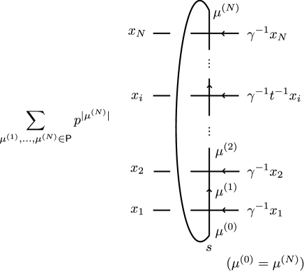
Figure 7: $\widetilde{\mathcal{T}}^{\mathrm{loop}}_{i}(\boldsymbol{x},p;s)$.

Definition 3.15.

Define $\widetilde{\mathcal{T}}^{\mathrm{loop}}_{i}(\boldsymbol{x},p;s)\colon\mathcal{F}^{(N,0)}_{\gamma^{-1}t^{-\delta_{i}}\cdot\boldsymbol{x}}\rightarrow\mathcal{F}^{(N,0)}_{\boldsymbol{x}}$ by

$$\widetilde{\mathcal{T}}^{\mathrm{loop}}_{i}(\boldsymbol{x},p;s)=\sum_{\begin{subarray}{c}\mu^{(1)},\ldots,\mu^{(N)}\in\mathsf{P}\\ (\mu^{(0)}=\mu^{(N)})\end{subarray}}p^{|\mu^{(N)}|}\bigotimes^{\curvearrowright}_{1\leq k\leq N}\Phi^{\mathrm{cr}}\left[x_{k};{\frac{y_{1}\cdots y_{k}}{x_{1}\cdots x_{k}}s,\mu^{(k)}\atop\frac{y_{1}\cdots y_{k-1}}{x_{1}\cdots x_{k-1}}s,\mu^{(k-1)}};y_{k}\right]\Bigg{|}_{y_{k}\rightarrow\gamma^{-1}t^{-\delta_{i,k}}x_{k}}.$$

Definition 3.16.

Set the shifted screening currents

$$S_{i}(z)=\widetilde{S}^{(i)}\big{(}t^{-i/N}z\big{)},\qquad 0\leq i\leq N-1.$$

The screening currents $S_{i}(z)$ are the realization of the operator in Appendix B in the case of $\kappa=t^{-1}$. In Fact 3.11, we expressed $\widetilde{\mathcal{T}}^{V}_{i}$ by composition of screening currents $\widetilde{S}^{(i)}(z)$ and $\phi_{0}(z)$. In the affine case, we compose the screening currents as follow.

Definition 3.17.

Define the affine screened vertex operators

$$\phi_{i}(z)={:}\phi_{i-1}\big{(}t^{-{1}/{N}}z\big{)}S_{i}(z){:}\qquad(i=1,\ldots,N-1),$$

$$\phi_{i+N}(z)=\phi_{i}(z),$$

$$\phi^{i}_{\lambda}(z)=\phi_{i-\ell(\lambda)}\big{(}t^{-(\ell(\lambda)+1)/N}z\big{)}\prod^{\curvearrowleft}_{1\leq j\leq\ell(\lambda)}S_{i-j+1}\big{(}t^{-j/N}q^{\lambda_{j}}z\big{)},$$

$$\Phi^{i}_{\lambda}(z)=\left(\frac{(q/t;q)_{\infty}}{(q;q)_{\infty}}\right)^{\ell(\lambda)}\phi^{i}_{\lambda}(z).$$

The operator $\widetilde{\mathcal{T}}^{\mathrm{loop}}_{i}$ can be expressed as follows. This is an affine analogue of Fact 3.11.

Proposition 3.18.

Let $i=1,\ldots,N$. Then we have

$$\widetilde{\mathcal{T}}^{\mathrm{loop}}_{i}(\boldsymbol{x},p;s)=\sum_{\lambda\in\mathsf{P}}p^{|\lambda|^{(i-1)}}\Phi^{i-1}_{\lambda}\big{(}t^{i/N}s\big{)}\prod_{1\leq k\leq N}x_{k}^{|\lambda|^{(i-k)}-|\lambda|^{(i-k-1)}},$$ (3.2)

where $|\lambda|^{(i)}=\sum_{j\equiv i+1(\mathrm{mod}N)}\lambda_{j}$.

For the proof, we prepare two lemmas.

Lemma 3.19.

Let $i=1,\ldots,N$. For a partition $\lambda\in\mathsf{P}$, set $\mu^{(k)}=(\lambda_{j};\ 1\leq j\leq\ell(\lambda),\ i-j\equiv k\mod N)$. Then, we have

$$\prod_{1\leq k\leq N}\frac{N_{\mu^{(k-1)},\mu^{(k)}}(t^{\delta_{k,i}})}{N_{\mu^{(k)},\mu^{(k)}}(1)}=\frac{\mathsf{N}^{(0|N)}_{\lambda\lambda}\big{(}t|q,t^{-1/N}\big{)}}{\mathsf{N}^{(0|N)}_{\lambda\lambda}\big{(}1|q,t^{-1/N}\big{)}},$$

where $\mathsf{N}^{(k|N)}_{\lambda\mu}(z|q,\kappa)$ is defined in Definition 3.21.

The proof is given in Section C.1.

Lemma 3.20.

Let $i=1,\ldots,N$. Then we have

$$\Phi^{i-1}_{\lambda}(z)=t^{-|\lambda|^{(0)}}\frac{\mathsf{N}^{(0|N)}_{\lambda\lambda}\big{(}t|q,t^{-1/N}\big{)}}{\mathsf{N}^{(0|N)}_{\lambda\lambda}(1|q,t^{-1/N}\big{)}}{:}\phi^{i-1}_{\lambda}(z){:}.$$

The proof is given in [44, Section 2.5].

Proof of Proposition 3.18.

First, the Nekrasov factors $\prod_{k=1}^{N}N_{\mu^{(k-1)},\mu^{(k)}}\big{(}t^{\delta_{k,i}}\big{)}$ arise from the normal ordering product of the operator

$$\bigotimes^{\curvearrowright}_{1\leq k\leq N}\Phi^{\mathrm{cr}}\left[x_{k};{\frac{y_{1}\cdots y_{k}}{x_{1}\cdots x_{k}}s,\mu^{(k)}\atop\frac{y_{1}\cdots y_{k-1}}{x_{1}\cdots x_{k-1}}s,\mu^{(k-1)}};y_{k}\right]\Bigg{|}_{y_{k}\rightarrow\gamma^{-1}t^{-\delta_{i,k}}x_{k}}.$$

(See Fact 2.11.) In general, for partitions $\nu$ and $\rho$, we have $N_{\nu,\rho}(1)\neq 0$ (resp. $N_{\nu,\rho}(t)\neq 0$) if and only if $\nu\subset\rho$ (resp. $\bar{\nu}\subset\rho$). Here, we put $\bar{\nu}=(\nu_{2},\nu_{3},\ldots)$ for $\nu=(\nu_{1},\nu_{2},\nu_{3},\ldots)$. Thus the partitions $\mu^{(k)}$ in (3.15) are restricted by the cyclic interlacing conditions

$$\mu^{(k-1)}\subset\mu^{(k)},\qquad k=1,\ldots,N\qquad(k\neq i);$$

$$\bar{\mu}^{(i-1)}\subset\mu^{(i)}.$$

Therefore, the $\mu^{(k)}$’s can be expressed by the single partition

$$\lambda=\big{(}\mu^{(i-1)}_{1},\mu^{(i-2)}_{1},\ldots,\mu^{(1)}_{1},\mu^{(N)}_{1},\mu^{(N-1)}_{1},\ldots,\mu^{(i)}_{1},$$

$$\hphantom{\lambda=\big{(}}\mu^{(i-1)}_{2},\mu^{(i-2)}_{2},\ldots,\mu^{(1)}_{2},\mu^{(N)}_{2},\ldots,\mu^{(i)}_{2},\mu^{(i-1)}_{3},\ldots\big{)}.$$

By using this $\lambda$, the partitions $\mu^{(k)}$’s can be written as

$$\mu^{(k)}=(\lambda_{j};\ 1\leq j\leq\ell(\lambda),\ i-j\equiv k\mod N).$$

Recalling Proposition 3.2 and Definition 3.4, we have

$$\bigotimes^{\curvearrowright}_{1\leq k\leq N}\Phi^{\mathrm{cr}}\left[x_{k};{\frac{y_{1}\cdots y_{k}}{x_{1}\cdots x_{k}}s,\mu^{(k)}\atop\frac{y_{1}\cdots y_{k-1}}{x_{1}\cdots x_{k-1}}s,\mu^{(k-1)}};y_{k}\right]\Bigg{|}_{y_{k}\rightarrow\gamma^{-1}t^{-\delta_{i,k}}x_{k}}$$

$$\hphantom{\bigotimes^{\curvearrowright}_{1\leq k\leq N}\Phi^{\mathrm{cr}}}{}=\prod_{1\leq k\leq N}N_{\mu^{(k-1)},\mu^{(k)}}\big{(}t^{\delta_{k,i}}\big{)}\frac{q^{2n(\mu^{(k)^{\prime}})}}{c_{\mu^{(k)}}c^{\prime}_{\mu^{(k)}}}\big{(}\gamma^{-1}t^{-\delta_{k,i}}x_{k}\big{)}^{|\mu^{(k-1)}|}f^{-1}_{\mu^{(k-1)}}q^{|\mu^{(k)}|}x_{k}^{-|\mu^{(k)}|}$$

$$\hphantom{\bigotimes^{\curvearrowright}_{1\leq k\leq N}\Phi^{\mathrm{cr}}\quad}{}\times{:}\phi_{0}(t^{-l^{\prime}}s)\prod_{k=1}^{i-1}\prod_{\alpha=0}^{l^{\prime}}\widetilde{S}^{(k)}\big{(}q^{\mu^{(k)}_{\alpha+1}}t^{-\alpha}s\big{)}\prod_{\alpha=0}^{l^{\prime}-1}\widetilde{S}^{(0)}\big{(}q^{\mu^{(0)}_{\alpha+1}}t^{-\alpha}s\big{)}$$

$$\hphantom{\bigotimes^{\curvearrowright}_{1\leq k\leq N}\Phi^{\mathrm{cr}}\quad}{}\times\prod_{k=i}^{N-1}\prod_{\alpha=1}^{l^{\prime}}\widetilde{S}^{(k)}\big{(}q^{\mu^{(k)}_{\alpha}}t^{-\alpha}s\big{)}{:},$$ (3.3)

where we put $l^{\prime}=\big{\lfloor}\frac{\ell(\lambda)-i}{N}\big{\rfloor}+1$. For $a\in\mathbb{Q}$, $\lfloor a\rfloor$ is defined to be the integer $n$ satisfying $n\leq a<n+1$. Lemma 3.19 and the equation

$$c_{\lambda}c^{\prime}_{\lambda}=(-1)^{(|\lambda|)}q^{n(\lambda^{\prime})+|\lambda|}t^{n(\lambda)}N_{\lambda,\lambda}(1)$$

show that

$$\prod_{1\leq k\leq N}N_{\mu^{(k-1)},\mu^{(k)}}(t^{\delta_{k,i}})\frac{q^{2n(\mu^{(k)^{\prime}})}}{c_{\mu^{(k)}}c^{\prime}_{\mu^{(k)}}}\big{(}\gamma^{-1}t^{-\delta_{k,i}}x_{k}\big{)}^{|\mu^{(k-1)}|}f^{-1}_{\mu^{(k-1)}}q^{|\mu^{(k)}|}x_{k}^{-|\mu^{(k)}|}$$

$$\hphantom{\prod_{1\leq k\leq N}}{}=t^{-|\lambda|^{(0)}}\frac{\mathsf{N}^{(0)}_{\lambda\lambda}\big{(}t|q,t^{-1/N}\big{)}}{\mathsf{N}^{(0)}_{\lambda\lambda}\big{(}1|q,t^{-1/N}\big{)}}\prod_{1\leq k\leq N}x_{k}^{|\lambda|^{(i-k)}-|\lambda|^{(i-k-1)}}.$$

Furthermore, by using the shifted screening current $S_{k}(z)$’s, the operator part in (3.3) can be rewritten as

$${:}\phi_{0}(t^{-l^{\prime}}s)\prod_{k=1}^{i-1}\prod_{\alpha=0}^{l^{\prime}}\widetilde{S}^{(k)}\big{(}q^{\mu^{(k)}_{\alpha+1}}t^{-\alpha}s\big{)}\prod_{\alpha=0}^{l^{\prime}-1}\widetilde{S}^{(0)}\big{(}q^{\mu^{(0)}_{\alpha+1}}t^{-\alpha}s\big{)}\prod_{k=i}^{N-1}\prod_{\alpha=1}^{l^{\prime}}\widetilde{S}^{(k)}\big{(}q^{\mu^{(k)}_{\alpha}}t^{-\alpha}s\big{)}{:}$$

$$\hphantom{{:}\phi_{0}(t^{-l^{\prime}}s)}{}={:}\phi_{0}\big{(}t^{-l^{\prime}}s\big{)}S_{i-\ell(\lambda)-1}\big{(}t^{-l^{\prime}}t^{[i-\ell(\lambda)-1]/N}s\big{)}\cdots S_{2}\big{(}t^{-l^{\prime}}t^{2/N}\big{)}S_{1}\big{(}t^{-l^{\prime}}t^{1/N}s\big{)}$$

$$\hphantom{{:}\phi_{0}(t^{-l^{\prime}}s)={:}}{}\times\prod_{1\leq j\leq\ell(\lambda)}S_{i-j}\big{(}t^{-j/N}q^{\lambda_{j}}t^{i/N}s\big{)}{:}={:}\phi^{i-1}_{\lambda}\big{(}t^{i/N}s\big{)}{:}.$$

Here, [a] is the integer satisfying that $0\leq[a]<N$ and $[a]\equiv a\mod N$. Therefore, by Lemma 3.20, we can show that (3.3) coincides with the RHS of (3.2). ∎

This proposition says that the vertex operators $\widetilde{\mathcal{T}}^{\mathrm{loop}}_{i}(\boldsymbol{x},p;s)$ can be identified with the screened vertex operators which are used to construct the non-stationary Ruijsenaars function in [44], though in our case, $\kappa$ should be specialized to $t^{-1/N}$. (See Appendix B.) This motivates us to state the affine analogue of Fact 3.13, that is, to construct the non-stationary Ruijsenaars function as the matrix element of the composition of $\widetilde{\mathcal{T}}^{\mathrm{loop}}_{i}(\boldsymbol{x},p;s)$’s.

In order to state the claim, we introduce the non-stationary Ruijsenaars function.

Definition 3.21 ([44]).

Let $\boldsymbol{s}=(s_{1},\ldots,s_{N})$, $\boldsymbol{x}=(x_{1},\ldots,x_{N})$ be $N$-tuples of indeterminates. Define $f^{\widehat{\mathfrak{gl}}_{N}}(\boldsymbol{x},p|\boldsymbol{s},\kappa|q,t)$ in $\mathbb{Q}(q,t,\boldsymbol{s})[[px_{2}/x_{1},\ldots,px_{N}/x_{N-1},px_{1}/x_{N}]]$ by

$$f^{\widehat{\mathfrak{gl}}_{N}}(\boldsymbol{x},p|\boldsymbol{s},\kappa|q,t)=\sum_{\lambda^{(1)},\ldots,\lambda^{(N)}\in{\mathsf{P}}}\prod_{i,j=1}^{N}{\mathsf{N}^{(j-i|N)}_{\lambda^{(i)},\lambda^{(j)}}(ts_{j}/s_{i}|q,\kappa)\over\mathsf{N}^{(j-i|N)}_{\lambda^{(i)},\lambda^{(j)}}(s_{j}/s_{i}|q,\kappa)}\prod_{\beta=1}^{N}\prod_{\alpha\geq 1}(px_{\alpha+\beta}/tx_{\alpha+\beta-1})^{\lambda^{(\beta)}_{\alpha}}.$$

We cyclically identify $x_{i+N}=x_{i}$ and put

$$\mathsf{N}^{(k|N)}_{\lambda,\mu}(u|q,\kappa)=\mathsf{N}^{(k)}_{\lambda,\mu}(u|q,\kappa)$$

$$\hphantom{\mathsf{N}^{(k|N)}_{\lambda,\mu}(u|q,\kappa)}{}=\!\!\!\prod_{j\geq i\geq 1\atop j-i\equiv k({\rm mod}N)}\!\!\!\!\!\big{(}uq^{-\mu_{i}+\lambda_{j+1}}\kappa^{-i+j};q\big{)}_{\lambda_{j}-\lambda_{j+1}}\!\!\!\!\!\!\!\prod_{\beta\geq\alpha\geq 1\atop\beta-\alpha\equiv-k-1({\rm mod}N)}\!\!\!\!\!\!\!\!\!\!\!\big{(}uq^{\lambda_{\alpha}-\mu_{\beta}}\kappa^{\alpha-\beta-1};q\big{)}_{\mu_{\beta}-\mu_{\beta+1}}.$$

Then, we obtain the following theorem. (See also Fig. 8.)

Figure 8: Non-stationary Ruijsenaars function $f^{\widehat{\mathfrak{gl}}_{N}}\big{(}\boldsymbol{x}^{\prime},p^{{1}/{N}}|\boldsymbol{s}^{\prime},t^{-{1}/{N}}|q,t\big{)}$.

Theorem 3.22.

Let

$$\boldsymbol{x}^{(i)}=\big{(}\gamma^{-i}t^{-1}x_{1},\ldots,\gamma^{-i}t^{-1}x_{i},\gamma^{-i}x_{i+1},\ldots,\gamma^{-i}x_{N}\big{)},\qquad 0\leq i\leq N.$$

Then we obtain

$$\bra{\boldsymbol{0}}\widetilde{\mathcal{T}}^{\mathrm{loop}}_{1}\big{(}\boldsymbol{x}^{(0)},p;s_{1}\big{)}\widetilde{\mathcal{T}}^{\mathrm{loop}}_{2}\big{(}\boldsymbol{x}^{(1)},p;s_{2}\big{)}\cdots\widetilde{\mathcal{T}}^{\mathrm{loop}}_{N}\big{(}\boldsymbol{x}^{(N-1)},p;s_{N}\big{)}\ket{\boldsymbol{0}}$$

$$\hphantom{\bra{\boldsymbol{0}}\widetilde{\mathcal{T}}^{\mathrm{loop}}_{1}\big{(}}{}=\prod_{1\leq i<j\leq N}\frac{(qs_{j}/s_{i};q)_{\infty}}{(ts_{j}/s_{i};q)_{\infty}}\,f^{\widehat{\mathfrak{gl}}_{N}}\big{(}\boldsymbol{x}^{\prime},p^{{1}/{N}}|\boldsymbol{s}^{\prime},t^{-{1}/{N}}|q,t\big{)}.$$

Here, we set

$$\boldsymbol{s}^{\prime}=(s^{\prime}_{1},\ldots,s^{\prime}_{N}),\qquad s^{\prime}_{k}=t^{{k}/{N}}s_{k},$$

$$\boldsymbol{x}^{\prime}=(x^{\prime}_{1},\ldots,x^{\prime}_{N}),\qquad x^{\prime}_{k}=p^{-{k}/{N}}x_{k}.$$

Proof.

Proposition 3.18 gives

$$\bra{\boldsymbol{0}}\widetilde{\mathcal{T}}^{\mathrm{loop}}_{1}\big{(}\boldsymbol{x}^{(0)},p;s_{1}\big{)}\widetilde{\mathcal{T}}^{\mathrm{loop}}_{2}\big{(}\boldsymbol{x}^{(1)},p;s_{2}\big{)}\cdots\widetilde{\mathcal{T}}^{\mathrm{loop}}_{N}\big{(}\boldsymbol{x}^{(N-1)},p;s_{N}\big{)}\ket{\boldsymbol{0}}$$

$$\hphantom{\bra{\boldsymbol{0}}\widetilde{\mathcal{T}}^{\mathrm{loop}}_{1}\big{(}}{}=\sum_{\lambda^{(1)},\ldots,\lambda^{(N)}}\bra{\boldsymbol{0}}\Phi^{0}_{\lambda^{(1)}}\big{(}t^{1/N}s_{1}\big{)}\Phi^{1}_{\lambda^{(2)}}\big{(}t^{2/N}s_{2}\big{)}\cdots\Phi^{N-1}_{\lambda^{(N)}}\big{(}t^{N/N}s_{N}\big{)}\ket{\boldsymbol{0}}$$

$$\hphantom{\bra{\boldsymbol{0}}\widetilde{\mathcal{T}}^{\mathrm{loop}}_{1}\big{(}=}{}\times\prod_{i=1}^{N}\prod_{k=1}^{N}(\gamma^{-i+1}t^{-\delta_{k\leq i-1}}x_{k})^{|\lambda^{(i)}|^{(i-k)}-|\lambda^{(i)}|^{(i-k-1)}}\prod_{i=1}^{N}p^{|\lambda^{(i)}|^{(i-1)}}.$$ (3.4)

Here, $\delta_{a\leq b}$ is $1$ if $a\leq b$ or $0$ if $a>b$. Then, we have

$$\prod_{i=1}^{N}\prod_{k=1}^{N}(\gamma^{-i+1})^{|\lambda^{(i)}|^{(i-k)}-|\lambda^{(i)}|^{(i-k-1)}}=1,$$

$$\prod_{i=1}^{N}\prod_{k=1}^{N}(t^{-\delta_{k\leq i-1}})^{|\lambda^{(i)}|^{(i-k)}-|\lambda^{(i)}|^{(i-k-1)}}=\prod_{i=1}^{N}t^{-|\lambda^{(i)}|^{(i-1)}+|\lambda^{(i)}|^{(0)}}$$

and

$$\prod_{i=1}^{N}\prod_{k=1}^{N}x_{k}^{|\lambda^{(i)}|^{(i-k)}-|\lambda^{(i)}|^{(i-k-1)}}\prod_{i=1}^{N}p^{|\lambda^{(i)}|^{(i-1)}}=\prod_{i=1}^{N}\prod_{j=1}^{\ell(\lambda^{(i)})}(x_{i-j+1}/x_{i-j})^{\lambda^{(i)}_{j}}\prod_{i=1}^{N}p^{|\lambda^{(i)}|^{(i-1)}}$$

$$\hphantom{\prod_{i=1}^{N}\prod_{k=1}^{N}x_{k}^{|\lambda^{(i)}|^{(i-k)}-|\lambda^{(i)}|^{(i-k-1)}}\prod_{i=1}^{N}p^{|\lambda^{(i)}|^{(i-1)}}}{}=\prod_{i=1}^{N}\prod_{j=1}^{\ell(\lambda^{(i)})}(p^{1/N}x^{\prime}_{i-j+1}/x^{\prime}_{i-j})^{\lambda^{(i)}_{j}}.$$

Therefore, Fact B.4 shows that (3.4) is equal to

$$\prod_{1\leq i<j\leq N}\frac{(qs_{j}/s_{i};q)_{\infty}}{(ts_{j}/s_{i};q)_{\infty}}\,f^{\widehat{\mathfrak{gl}}_{N}}\big{(}(1/x^{\prime}_{N},\ldots,1/x^{\prime}_{1}),p^{{1}/{N}}\big{|}(1/s^{\prime}_{N},\ldots,1/s^{\prime}_{N}),t^{-{1}/{N}}\big{|}q,t\big{)}.$$ (3.5)

Finally, it can be easily shown that the non-stationary Ruijsenaars function in (3.5) coincides with $f^{\widehat{\mathfrak{gl}}_{N}}\big{(}\boldsymbol{x}^{\prime},p^{{1}/{N}}|\boldsymbol{s}^{\prime},t^{-{1}/{N}}|q,t\big{)}$. ∎

Remark 3.23.

The LHS in this theorem can be rewritten by the trace of the operators $\widetilde{\mathcal{T}}^{H}$. For an operator $A\in\mathrm{End}\big{(}(\mathcal{F}^{(0,1)})^{\otimes N}\big{)}$, set the formal power series

$$\mathrm{Tr}_{p}(A)=\sum_{\boldsymbol{\lambda}\in\mathsf{P}^{N}}p^{|\boldsymbol{\lambda}|}\bra{\boldsymbol{\lambda}}A\ket{\boldsymbol{\lambda}}.$$

Then it is clear that

$$\bra{\boldsymbol{0}}\widetilde{\mathcal{T}}^{\mathrm{loop}}_{1}\big{(}\boldsymbol{x}^{(0)},p;s_{1}\big{)}\cdots\widetilde{\mathcal{T}}^{\mathrm{loop}}_{N}\big{(}\boldsymbol{x}^{(N-1)},p;s_{N}\big{)}\ket{\boldsymbol{0}}=\mathrm{Tr}_{p}\big{(}\widetilde{\mathcal{T}}^{H}_{N}\big{(}\boldsymbol{s}^{(N-1)};x_{N}\big{)}\cdots\widetilde{\mathcal{T}}^{H}_{1}\big{(}\boldsymbol{s}^{(0)};x_{1}\big{)}\big{)}.$$

Here,

$$\boldsymbol{s}^{(i)}=\big{(}\gamma^{-i}t^{-1}s_{1},\ldots,\gamma^{-i}t^{-1}s_{i},\gamma^{-i}s_{i+1},\ldots,\gamma^{-i}s_{N}\big{)},\qquad 0\leq i\leq N.$$

3.2 Lift to elliptic hypergeometric series
and non-stationary Ruijsenaars function

In the previous subsection, we took the loop at vertical direction of the reticulate diagram. Next, we calculate a loop at horizontal direction. This loop can reproduce the lift $f^{\mathrm{ellip}}_{N}(\boldsymbol{x},\boldsymbol{s}|q,t,p)$ of the Macdonald function $f^{\mathfrak{gl}_{N}}$ by the elliptic gamma functions. Let us recall the definition of $f^{\mathrm{ellip}}_{N}(\boldsymbol{x},\boldsymbol{s}|q,t,p)$.

Definition 3.24.

Define $f^{\mathrm{ellip}}_{N}(\boldsymbol{x};\boldsymbol{s}|q,t,p)\in\mathbb{Q}(q,t,\boldsymbol{s})[[p,x_{2}/x_{1},\ldots,x_{N}/x_{N-1}]]$ by

$$f^{\mathrm{ellip}}_{N}(\boldsymbol{x};\boldsymbol{s}|q,t,p)=\sum_{\theta\in\mathsf{M}_{N}}c^{\mathrm{ellip}}_{N}(\theta;\boldsymbol{s}|q,q/t,p)\prod_{1\leq i<j\leq N}(x_{j}/x_{i})^{\theta_{ij}},$$

where

$$c^{\mathrm{ellip}}_{N}(\theta;\boldsymbol{s}|q,t,p)=\prod_{k=2}^{N}\prod_{1\leq i<j\leq k}\dfrac{\Theta(q^{\sum_{a>k}(\theta_{ia}-\theta_{ja})}ts_{j}/s_{i};q,p)_{\theta_{ik}}}{\Theta(q^{\sum_{a>k}(\theta_{ia}-\theta_{ja})}qs_{j}/s_{i};q,p)_{\theta_{ik}}}$$

$$\hphantom{c^{\mathrm{ellip}}_{N}(\theta;\boldsymbol{s}|q,t,p)=}\times\prod_{k=2}^{N}\prod_{1\leq i\leq j<k}\dfrac{\Theta(q^{-\theta_{jk}+\sum_{a>k}(\theta_{ia}-\theta_{ja})}qs_{j}/ts_{i};q,p)_{\theta_{ik}}}{\Theta(q^{-\theta_{jk}+\sum_{a>k}(\theta_{ia}-\theta_{ja})}s_{j}/s_{i};q,p)_{\theta_{ik}}}.$$

$\Theta(-;q,p)_{n}$ is defined in (1.2).

It is clear that the function $f^{\mathrm{ellip}}_{N}(\boldsymbol{x},\boldsymbol{s}|q,t,p)$ is reduced to the ordinary Macdonald function, i.e.,

$$f^{\mathrm{ellip}}_{N}(\boldsymbol{x},\boldsymbol{s}|q,t,p)\underset{p\rightarrow 0}{\longrightarrow}f^{\mathfrak{gl}_{N}}(\boldsymbol{x},\boldsymbol{s}|q,q/t).$$

We give a realization of this elliptic lift by taking the trace of the Mukadé operators.

Definition 3.25.

For $A\in\mathrm{End}(\mathcal{F}^{\otimes N})$, define the $p$-trace $\mathrm{tr}(p^{d}A)$ to be

$$\mathrm{tr}(p^{d}A)=\sum_{\boldsymbol{\lambda}\in\mathsf{P}^{N}}p^{|\boldsymbol{\lambda}|}\frac{\bra{a_{\boldsymbol{\lambda}}}A\ket{a_{\boldsymbol{\lambda}}}}{\braket{a_{\boldsymbol{\lambda}}}{a_{\boldsymbol{\lambda}}}}.$$

Note that the trace $\mathrm{tr}(p^{d}{-})$ certainly does not depend on bases.

Our main purpose in this subsection is to compute the trace of the following operator. See also Fig. 9.

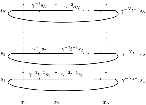
Figure 9: $\mathrm{tr}\big{(}p^{d}\widetilde{\mathcal{T}}^{N}(\boldsymbol{s};\boldsymbol{x})\big{)}$.

Definition 3.26.

Define the $N$-compositions of operators $\widetilde{\mathcal{T}}^{V}_{i}$ as

$$\widetilde{\mathcal{T}}^{N}(\boldsymbol{s};\boldsymbol{x}):=\widetilde{\mathcal{T}}^{V}_{1}\big{(}\boldsymbol{s}^{(0)};x_{1}\big{)}\widetilde{\mathcal{T}}^{V}_{2}\big{(}\boldsymbol{s}^{(1)};x_{2}\big{)}\cdots\widetilde{\mathcal{T}}^{V}_{N}\big{(}\boldsymbol{s}^{(N-1)};x_{N}\big{)},$$

where

$$\boldsymbol{s}^{(i)}=\big{(}\gamma^{-i}t^{-1}s_{1},\dots,\gamma^{-i}t^{-1}s_{i},\gamma^{-i}s_{i+1},\dots,\gamma^{-i}u_{N}\big{)}.$$ (3.6)

We state the key property of the $p$-trace.

Notation 3.27.

Write

$$\widehat{\mathcal{H}}^{N}[z]:=\left\{{\rm e}^{\sum_{r>0,1\leq i\leq N}R^{(i)}_{-r}a^{(i)}_{-r}z^{r}}{\rm e}^{\sum_{r>0,1\leq i\leq N}R^{(i)}_{r}a^{(i)}_{r}z^{-r}}\in\mathrm{End}\big{(}\mathcal{F}^{\otimes N}\big{)}\big{[}\big{[}z^{\pm 1}\big{]}\big{]}\,|\,R^{(i)}_{r}\in\mathbb{C}\right\}.$$

Lemma 3.28.

Let $A_{i}(z)\in\widehat{\mathcal{H}}^{N}[z]$ $(i=1,\ldots,n)$ be operators which satisfy

$$A_{i}(z)A_{j}(w)=\prod_{l}\frac{1-a^{i,j}_{l}w/z}{1-b^{i,j}_{l}w/z}{:}A_{i}(z)A_{j}(w){:}\qquad(a^{i,j}_{l},b^{i,j}_{l}\in\mathbb{C},\;i,j=1,\ldots,n),$$

where the product with respect to $l$ can be either finite or infinite if it converges. Then, it follows that

$$\mathrm{tr}\big{(}p^{d}A_{1}(z_{1})\cdots A_{n}(z_{n})\big{)}=\frac{1}{(p;p)_{\infty}^{N}}\prod_{1\leq i<j\leq n}\prod_{l}\frac{(a^{i,j}_{l}z_{j}/z_{i};p)_{\infty}}{(b^{i,j}_{l}z_{j}/z_{i};p)_{\infty}}\prod_{1\leq j\leq i\leq n}\prod_{l}\frac{(pa^{i,j}_{l}z_{j}/z_{i};p)_{\infty}}{(pb^{i,j}_{l}z_{j}/z_{i};p)_{\infty}}.$$

In particular, if the operators satisfy

$$A_{1}(z)A_{2}(w)=\frac{(aw/z;q)_{\infty}}{(bw/z;q)_{\infty}}{:}A_{1}(z)A_{2}(w){:},\quad\ A_{2}(w)A_{1}(z)=\frac{(qz/bw;q)_{\infty}}{(qz/aw;q)_{\infty}}{:}A_{2}(w)A_{1}(z){:},$$

then we can rewrite the result by the elliptic gamma functions:

$$\mathrm{tr}\big{(}p^{d}A_{1}(z)A_{2}(w)\big{)}=\frac{1}{(p;p)_{\infty}^{N}}\frac{\Gamma(bw/z;q,p)}{\Gamma(aw/z;q,p)}\prod_{i=1}^{2}\prod_{l}\frac{(pa^{i,i}_{l};p)_{\infty}}{(pb^{i,i}_{l};p)_{\infty}}.$$

Proof.

Let $A^{\pm}_{i}(z)$ be the operators of the forms

$$A^{-}_{i}(z)={\rm e}^{\sum_{r>0,1\leq i\leq N}R^{(i)}_{-r}a^{(i)}_{-r}z^{r}},\qquad A^{+}_{i}(z)={\rm e}^{\sum_{r>0,1\leq i\leq N}R^{(i)}_{r}a^{(i)}_{r}z^{-r}}\qquad\big{(}R^{(i)}_{\pm r}\in\mathbb{C}\big{)}$$

such that $A_{i}(z)=A^{-}_{i}(z)A^{+}_{i}(z)$. Then we have

$$\mathrm{tr}\big{(}p^{d}A_{1}(z_{1})\cdots A_{n}(z_{n})\big{)}$$

$$\qquad{}=\prod_{1\leq i<j\leq n}\prod_{l}\frac{1-a^{i,j}_{l}z_{j}/z_{i}}{1-b^{i,j}_{l}z_{j}/z_{i}}\,\mathrm{tr}\big{(}p^{d}A^{-}_{1}(z_{1})\cdots A^{-}_{n}(z_{n})A^{+}_{1}(z_{1})\cdots A^{+}_{n}(z_{n})\big{)}$$

$$\qquad{}=\prod_{1\leq i<j\leq n}\prod_{l}\frac{1-a^{i,j}_{l}z_{j}/z_{i}}{1-b^{i,j}_{l}z_{j}/z_{i}}\,\mathrm{tr}\big{(}p^{d}A^{+}_{1}\big{(}p^{-1}z_{1}\big{)}\cdots A^{+}_{n}(p^{-1}z_{n})A^{-}_{1}(z_{1})\cdots A^{-}_{n}(z_{n})\big{)}$$

$$\qquad{}=\prod_{1\leq i<j\leq n}\prod_{l}\frac{1-a^{i,j}_{l}z_{j}/z_{i}}{1-b^{i,j}_{l}z_{j}/z_{i}}\prod_{i,j=1}^{n}\prod_{l}\frac{1-pa^{i,j}_{l}z_{j}/z_{i}}{1-pb^{i,j}_{l}z_{j}/z_{i}}$$

$$\phantom{\qquad{}=\prod_{1\leq i<j\leq n}}\times\mathrm{tr}\big{(}p^{d}A^{-}_{1}(z_{1})\cdots A^{-}_{n}(z_{n})A^{+}_{1}\big{(}p^{-1}z_{1}\big{)}\cdots A^{+}_{n}\big{(}p^{-1}z_{n}\big{)}\big{)}.$$

Since $\mathrm{tr}(p^{d}\cdot 1)=\frac{1}{(p;p)^{N}_{\infty}}$, by repeating the calculation above, it can shown that for any $m\in\mathbb{Z}_{>0}$,

$$\mathrm{tr}\big{(}p^{d}A_{1}(z_{1})\cdots A_{n}(z_{n})\big{)}$$

$$\qquad{}=\frac{1}{(p;p)_{\infty}^{N}}\prod_{1\leq i<j\leq n}\prod_{l}\frac{\big{(}a^{i,j}_{l}z_{j}/z_{i};p\big{)}_{m}}{\big{(}b^{i,j}_{l}z_{j}/z_{i};p\big{)}_{m}}\prod_{1\leq j\leq i\leq n}\prod_{l}\frac{\big{(}pa^{i,j}_{l}z_{j}/z_{i};p\big{)}_{m}}{\big{(}pb^{i,j}_{l}z_{j}/z_{i};p\big{)}_{m}}+\mathcal{O}(p^{m}).$$

This completes the proof. ∎

Proposition 3.29.

We obtain

$$\mathrm{tr}\big{(}p^{d}\widetilde{\mathcal{T}}^{N}(\boldsymbol{s};\boldsymbol{x})\big{)}=\left(\frac{(pq/t;q,p)_{\infty}}{(p;p)_{\infty}(pt;q,p)_{\infty}}\right)^{N}\prod_{1\leq i<j\leq N}\frac{\Gamma(tx_{j}/x_{i};q,p)}{\Gamma(qx_{j}/x_{i};q,p)}\,f^{\mathrm{ellip}}_{N}(\boldsymbol{s};\boldsymbol{x}|q,t,p).$$

Proof.

Using Fact 3.11 and Lemma 3.28, we can compute the trace as

$$\mathrm{tr}\big{(}p^{d}\widetilde{\mathcal{T}}^{N}(\boldsymbol{s};\boldsymbol{x})\big{)}$$

$$\hphantom{\mathrm{tr}\big{(}}{}=\left(\frac{(q/t;q)_{\infty}}{(q;q)_{\infty}}\right)^{N(N-1)/2}(p;p)^{N(N-3)/2}\left(\frac{(pq/t;q,p)_{\infty}}{(pt;q,p)_{\infty}}\right)^{N(N+1)/2}$$

$$\hphantom{\mathrm{tr}\big{(}=}{}\times\prod_{1\leq i<j\leq N}\frac{\Gamma(tx_{j}/x_{i};q,p)}{\Gamma(qx_{j}/tx_{i};q,p)}\sum_{(m_{i,j})_{1\leq i<j\leq N}}\prod_{1\leq i<j\leq N}\frac{\Gamma(qq^{m_{i,j}-m_{i-1,j}}/t;q,p)}{\Gamma(qq^{m_{i,j}-m_{i-1,j}};q,p)}$$

$$\hphantom{\mathrm{tr}\big{(}=}\times\prod_{1\leq i<j\leq N}\frac{\Gamma(qq^{m_{1,j}}x_{j}/tx_{i};q,p)}{\Gamma(qq^{m_{1,j}}x_{j}/x_{i};q,p)}$$

$$\hphantom{\mathrm{tr}\big{(}=}\times\prod_{k=2}^{N-1}\prod_{k\leq i<j\leq N}\frac{\Gamma(qq^{m_{k-1,j}-m_{k-1,i}}x_{j}/x_{i};q,p)}{\Gamma(q^{m_{k-1,j}-m_{k-1,i}}x_{j}/x_{i};q,p)}\frac{\Gamma(tq^{m_{k-1,j}-m_{k-1,i}}x_{j}/x_{i};q,p)}{\Gamma(qq^{m_{k-1,j}-m_{k-1,i}}x_{j}/tx_{i};q,p)}$$

$$\hphantom{\mathrm{tr}\big{(}=}\times\prod_{k=2}^{N-1}\prod_{k\leq i<j\leq N}\frac{\Gamma(q^{m_{k-2,j}-m_{k-1,i}}x_{j}/x_{i};q,p)}{\Gamma(tq^{m_{i-2,j}-m_{k-1,i}}x_{j}/x_{i};q,p)}\frac{\Gamma(qq^{m_{k,j}-m_{k-1,i}}x_{j}/tx_{i};q,p)}{\Gamma(qq^{m_{k,j}-m_{k-1,i}}x_{j}/x_{i};q,p)}$$

$$\hphantom{\mathrm{tr}\big{(}=}\times\prod_{k=2}^{N}\prod_{i=1}^{k-1}\big{(}t^{\delta_{i,k-1}}s_{i+1}/s_{i}\big{)}^{m_{i,k}}.$$

Here, the summation runs over all integers such that $m_{j-1,j}\geq m_{j-2,j}\geq\cdots\geq m_{1,j}\geq 0$ ($j=2,\ldots,N$). Then, it can be shown that

$$\left(\frac{(q/t;q)_{\infty}}{(q;q)_{\infty}}\right)^{N(N-1)/2}(p;p)^{N(N-3)/2}\left(\frac{(pq/t;q,p)_{\infty}}{(pt;q,p)_{\infty}}\right)^{N(N+1)/2}$$

$$\qquad=\left(\frac{\Gamma(q;q,p)}{\Gamma(q/t;q,p)}\right)^{N(N-1)/2}\left(\frac{(pq/t;q,p)_{\infty}}{(p;p)_{\infty}(pt;q,p)_{\infty}}\right)^{N}.$$

Put $\theta_{1,j}:=m_{1,j}$ ($j=2,\ldots,N$) and $\theta_{i,j}:=m_{i,j}-m_{i-1,j}$ ($j\geq 3$, $i=2,\ldots,j-1$). We have

$$\left(\frac{\Gamma(q;q,p)}{\Gamma(q/t;q,p)}\right)^{N(N-1)/2}\prod_{1\leq i<j\leq N}\frac{\Gamma(qq^{m_{i,j}-m_{i-1,j}}/t;q,p)}{\Gamma(qq^{m_{i,j}-m_{i-1,j}};q,p)}=\prod_{1\leq i<j\leq N}\frac{\Theta(q/t;q,p)_{\theta_{i,j}}}{\Theta(q;q,p)_{\theta_{i,j}}},$$

$$\prod_{1\leq i<j\leq N}\frac{\Gamma(qq^{m_{1,j}}x_{j}/tx_{i};q,p)}{\Gamma(qq^{m_{1,j}}x_{j}/x_{i};q,p)}=\prod_{1\leq i<j\leq N}\frac{\Theta(qx_{j}/tx_{i};q,p)_{\theta_{1,j}}}{\Theta(qx_{j}/x_{i};q,p)_{\theta_{1,j}}}\frac{\Gamma(qx_{j}/tx_{i};q,p)}{\Gamma(qx_{j}/x_{i};q,p)}$$

and

$$\prod_{k=2}^{N-1}\prod_{k\leq i<j\leq N}\frac{\Gamma(qq^{m_{k-1,j}-m_{k-1,i}}x_{j}/x_{i};q,p)}{\Gamma(q^{m_{k-1,j}-m_{k-1,i}}x_{j}/x_{i};q,p)}\frac{\Gamma(tq^{m_{k-1,j}-m_{k-1,i}}x_{j}/x_{i};q,p)}{\Gamma(qq^{m_{k-1,j}-m_{k-1,i}}x_{j}/tx_{i};q,p)}$$

$$\quad\times\prod_{k=2}^{N-1}\prod_{k\leq i<j\leq N}\frac{\Gamma(q^{m_{k-2,j}-m_{k-1,i}}x_{j}/x_{i};q,p)}{\Gamma(tq^{m_{i-2,j}-m_{k-1,i}}x_{j}/x_{i};q,p)}\frac{\Gamma(qq^{m_{k,j}-m_{k-1,i}}x_{j}/tx_{i};q,p)}{\Gamma(qq^{m_{k,j}-m_{k-1,i}}x_{j}/x_{i};q,p)}$$

$$\quad=\prod_{k=2}^{N-1}\prod_{k\leq i<j\leq N}\!\!\frac{\Theta(tq^{m_{k-2,j}-m_{k-1,i}}x_{j}/x_{i};q,p)_{\theta_{k-1,j}}}{\Theta(q^{m_{k-2,j}-m_{k-1,i}}x_{j}/x_{i};q,p)_{\theta_{k-1,j}}}\frac{\Theta(qq^{m_{k-1,j}-m_{k-1,i}}x_{j}/tx_{i};q,p)_{\theta_{k,j}}}{\Theta(qq^{m_{k-1,j}-m_{k-1,i}}x_{j}/x_{i};q,p)_{\theta_{k,j}}}.\!\!$$ (3.7)

The exponent of $q$ in (3.7) can be rewritten as

$$m_{k-2,j}-m_{k-1,i}=-\theta_{k-1,i}+\sum_{a=1}^{k-2}(\theta_{a,j}-\theta_{a,i}),\qquad m_{k-1,j}-m_{k-1,i}=\sum_{a=1}^{k-1}(\theta_{a,j}-\theta_{a,i}).$$

Moreover, we have

$$\prod_{k=2}^{N}\prod_{i=1}^{k-1}\big{(}t^{\delta_{i,k-1}}s_{i+1}/s_{i}\big{)}^{m_{i,k}}=\prod_{1\leq i<j\leq N}t^{\theta_{i,j}}(s_{j}/s_{i})^{\theta_{i,j}}.$$

By the calculation above, we obtain

$$\mathrm{tr}\big{(}p^{d}\widetilde{\mathcal{T}}^{N}(\boldsymbol{s};\boldsymbol{x})\big{)}=\left(\frac{(pq/t;q,p)_{\infty}}{(p;p)_{\infty}(pt;q,p)_{\infty}}\right)^{N}\prod_{1\leq i<j\leq N}\frac{\Gamma(tx_{j}/x_{i};q,p)}{\Gamma(qx_{j}/x_{i};q,p)}$$

$$\hphantom{\mathrm{tr}\big{(}p^{d}\widetilde{\mathcal{T}}^{N}(\boldsymbol{s};\boldsymbol{x})\big{)}=}{}\times\sum_{\theta\in\mathsf{M}_{N}}\prod_{1\leq i<j\leq N}\frac{\Theta(q/t;q,p)_{\theta_{i,j}}}{\Theta(q;q,p)_{\theta_{i,j}}}\prod_{1\leq i<j\leq N}\frac{\Theta(qx_{j}/tx_{i};q,p)_{\theta_{1,j}}}{\Theta(qx_{j}/x_{i};q,p)_{\theta_{1,j}}}$$

$$\hphantom{\mathrm{tr}\big{(}p^{d}\widetilde{\mathcal{T}}^{N}(\boldsymbol{s};\boldsymbol{x})\big{)}=}{}\times\prod_{k=2}^{N-1}\prod_{k\leq i<j\leq N}\frac{\Theta(tq^{-\theta_{k-1,i}+\sum_{a=1}^{k-2}(\theta_{a,j}-\theta_{a,i})}x_{j}/x_{i};q,p)_{\theta_{k-1,j}}}{\Theta(q^{-\theta_{k-1,i}+\sum_{a=1}^{k-2}(\theta_{a,j}-\theta_{a,i})}x_{j}/x_{i};q,p)_{\theta_{k-1,j}}}$$

$$\hphantom{\mathrm{tr}\big{(}p^{d}\widetilde{\mathcal{T}}^{N}(\boldsymbol{s};\boldsymbol{x})\big{)}=}{}\times\frac{\Theta(qq^{\sum_{a=1}^{k-1}(\theta_{a,j}-\theta_{a,i})}x_{j}/tx_{i};q,p)_{\theta_{k,j}}}{\Theta(qq^{\sum_{a=1}^{k-1}(\theta_{a,j}-\theta_{a,i})}x_{j}/x_{i};q,p)_{\theta_{k,j}}}\prod_{1\leq i<j\leq N}t^{\theta_{i,j}}(s_{j}/s_{i})^{\theta_{i,j}}$$

$$\hphantom{\mathrm{tr}\big{(}p^{d}\widetilde{\mathcal{T}}^{N}(\boldsymbol{s};\boldsymbol{x})\big{)}}{}=\left(\frac{(pq/t;q,p)_{\infty}}{(p;p)_{\infty}(pt;q,p)_{\infty}}\right)^{N}\prod_{1\leq i<j\leq N}\frac{\Gamma(tx_{j}/x_{i};q,p)}{\Gamma(qx_{j}/x_{i};q,p)}$$

$$\hphantom{\mathrm{tr}\big{(}p^{d}\widetilde{\mathcal{T}}^{N}(\boldsymbol{s};\boldsymbol{x})\big{)}=}{}\times\sum_{\theta\in\mathsf{M}_{N}}\prod_{k=1}^{N-1}\prod_{k<i\leq j\leq N}\frac{\Theta(tq^{-\theta_{k,i}+\sum_{a=1}^{k-1}(\theta_{a,j}-\theta_{a,i})}x_{j}/x_{i};q,p)_{\theta_{k,j}}}{\Theta(q^{-\theta_{k,i}+\sum_{a=1}^{k-1}(\theta_{a,j}-\theta_{a,i})}x_{j}/x_{i};q,p)_{\theta_{k,j}}}$$

$$\hphantom{\mathrm{tr}\big{(}p^{d}\widetilde{\mathcal{T}}^{N}(\boldsymbol{s};\boldsymbol{x})\big{)}=}{}\times\prod_{k=1}^{N-1}\prod_{k\leq i<j\leq N}\frac{\Theta(qq^{\sum_{a=1}^{k-1}(\theta_{a,j}-\theta_{a,i})}x_{j}/tx_{i};q,p)_{\theta_{k,j}}}{\Theta(qq^{\sum_{a=1}^{k-1}(\theta_{a,j}-\theta_{a,i})}x_{j}/x_{i};q,p)_{\theta_{k,j}}}\prod_{1\leq i<j\leq N}(s_{j}/s_{i})^{\theta_{i,j}}.$$

Since $\theta_{i,j}$, $x_{i}$ and $s_{i}$ correspond to $\theta_{N-j+1,N-i+1}$, $1/s_{N-i+1}$ and $1/x_{N-i+1}$ in Definition 3.24, respectively, we have

$$\mathrm{tr}\big{(}p^{d}\widetilde{\mathcal{T}}^{N}(\boldsymbol{s};\boldsymbol{x})\big{)}=\left(\frac{(pq/t;q,p)_{\infty}}{(p;p)_{\infty}(pt;q,p)_{\infty}}\right)^{N}\prod_{1\leq i<j\leq N}\frac{\Gamma(tx_{j}/x_{i};q,p)}{\Gamma(qx_{j}/x_{i};q,p)}$$

$$\hphantom{\mathrm{tr}\big{(}p^{d}\widetilde{\mathcal{T}}^{N}(\boldsymbol{s};\boldsymbol{x})\big{)}=}{}\times f^{\mathrm{ellip}}_{N}(1/s_{N},\ldots,1/s_{1};1/x_{N},\ldots,1/x_{1}|q,q/t,p).$$

Therefore, Proposition 3.29 follows from the symmetry

$$f^{\mathrm{ellip}}_{N}(1/x_{N},\ldots,1/x_{1};1/s_{N},\ldots,1/s_{1}|q,t,p)=f^{\mathrm{ellip}}_{N}(x_{1},\ldots,x_{N};s_{1},\ldots,s_{N}|q,t,p).$$ ∎

Now, we obtain a relationship between the non-stationary Ruijsenaars functions and the functions $f^{\mathrm{ellip}}$.

Theorem 3.30.

As formal series in $p$, $s_{i+1}/s_{i}$, $x_{i+1}/x_{i}$ ($i=1,\ldots,N-1$) and $px_{1}/x_{N}$, we obtain

$$f^{\widehat{\mathfrak{gl}}_{N}}\big{(}\boldsymbol{x}{}^{\prime},p^{{1}/{N}}|\boldsymbol{s}^{\prime},t^{-{1}/{N}}|q,t\big{)}=\mathfrak{C}\times f^{\mathrm{ellip}}_{N}(\boldsymbol{s};\boldsymbol{x}|q,t,p),$$

where we put

$$\mathfrak{C}:=\left(\frac{(pq/t;q,p)_{\infty}}{(p;p)_{\infty}(pt;q,p)_{\infty}}\right)^{N}\prod_{1\leq i<j\leq N}\frac{\Gamma(tx_{j}/x_{i};q,p)}{\Gamma(qx_{j}/x_{i};q,p)}\prod_{1\leq i<j\leq N}\frac{(ts_{j}/s_{i};q)_{\infty}}{(qs_{j}/s_{i};q)_{\infty}}.$$

$\boldsymbol{x}^{\prime}$ and $\boldsymbol{s}^{\prime}$ are the same ones in Theorem 3.22:

$$\boldsymbol{s}^{\prime}=(s^{\prime}_{1},\ldots,s^{\prime}_{N}),\qquad s^{\prime}_{k}=t^{{k}/{N}}s_{k},$$

$$\boldsymbol{x}^{\prime}=(x^{\prime}_{1},\ldots,x^{\prime}_{N}),\qquad x^{\prime}_{k}=p^{-{k}/{N}}x_{k}.$$

For the proof, we prepare the following lemma.

Lemma 3.31.

Let $1\leq k\leq N$. The vacuum expectation values of the Mukadé operators are

$$\bra{\boldsymbol{\emptyset}}\widetilde{\mathcal{T}}^{H}_{k}\left(\boldsymbol{u},;x\right)\ket{\boldsymbol{\emptyset}}=\prod_{1\leq i<k}\frac{(qu_{k}/tu_{i};q)_{\infty}}{(u_{k}/u_{i};q)_{\infty}},\qquad\bra{\boldsymbol{0}}\widetilde{\mathcal{T}}^{V}_{k}(\boldsymbol{u};x)\ket{\boldsymbol{0}}=\prod_{i=1}^{k-1}\frac{(qu_{k}/tu_{i};q)_{\infty}}{(u_{k}/u_{i};q)_{\infty}}.$$

Proof.

The first vacuum expectation value can be directly calculated as

$$\bra{\boldsymbol{\emptyset}}\widetilde{\mathcal{T}}^{H}_{k}(\boldsymbol{u},;x)\ket{\boldsymbol{\emptyset}}=\prod_{1\leq i<j\leq N}\frac{\mathcal{G}(t^{-\delta_{j,k}+\delta_{i,k}}u_{j}/u_{i})}{\mathcal{G}(t^{\delta_{i,k}}u_{j}/u_{i})}\frac{\mathcal{G}(qu_{j}/tu_{i})}{\mathcal{G}(qt^{-\delta_{j,k}-1}u_{j}/u_{i})}$$

$$\hphantom{\bra{\boldsymbol{\emptyset}}\widetilde{\mathcal{T}}^{H}_{k}(\boldsymbol{u},;x)\ket{\boldsymbol{\emptyset}}}{}=\prod_{1\leq i<k}\frac{\mathcal{G}(u_{j}/tu_{i})}{\mathcal{G}(u_{j}/u_{i})}\frac{\mathcal{G}(qu_{j}/tu_{i})}{\mathcal{G}(qu_{j}/t^{2}u_{i})}=\prod_{1\leq i<k}\frac{(qu_{k}/tu_{i};q)_{\infty}}{(u_{k}/u_{i};q)_{\infty}}.$$

The second one can be calculated by using the $q$-binomial theorem:

$$\bra{\boldsymbol{0}}\widetilde{\mathcal{T}}^{V}_{k}(\boldsymbol{u};x)\ket{\boldsymbol{0}}=\left(\frac{(q/t;q)_{\infty}}{(q;q)_{\infty}}\right)^{k-1}\sum_{0\leq m_{1}\leq\cdots\leq m_{k-1}}\frac{(qq^{m_{1}};q)_{\infty}}{(qq^{m_{1}}/t;q)_{\infty}}\prod_{i=2}^{k-1}\frac{(qq^{m_{i}-m_{i-1}};q)_{\infty}}{(qq^{m_{i}-m_{i-1}}/t;q)_{\infty}}$$

$$\hphantom{\bra{\boldsymbol{0}}\widetilde{\mathcal{T}}^{V}_{k}(\boldsymbol{u};x)\ket{\boldsymbol{0}}=}{}\times\prod_{i=1}^{k-1}\left(\frac{u_{i+1}}{u_{i}}\right)^{m_{i}}=\sum_{n_{1},\ldots,n_{k-1}\in\mathbb{Z}_{\geq 0}}\prod_{i=1}^{k-1}\frac{(q/t;q)_{n_{i}}}{(q;q)_{n_{i}}}\prod_{i=1}^{k-1}\left(\frac{u_{k}}{u_{i}}\right)^{n_{i}}$$

$$\hphantom{\bra{\boldsymbol{0}}\widetilde{\mathcal{T}}^{V}_{k}(\boldsymbol{u};x)\ket{\boldsymbol{0}}}{}=\prod_{i=1}^{k-1}\frac{(qu_{k}/tu_{i};q)_{\infty}}{(u_{k}/u_{i};q)_{\infty}}.$$ ∎

Proof of Theorem 3.30.

In this proof, we use the same notation as in (3.6). For the sketch of the proof, see Fig. 3 in Introduction. By virtue of Theorem 2.24, we have

$$\mathrm{tr}\big{(}p^{d}\widetilde{\mathcal{T}}^{N}(\boldsymbol{s};\boldsymbol{x})\big{)}=\sum_{\boldsymbol{\mu}_{0},\ldots,\boldsymbol{\mu}_{N-1}\in\mathsf{P}^{N}}p^{|\boldsymbol{\mu}_{0}|}\prod_{i=1}^{N}\bra{P_{\boldsymbol{\mu}_{i-1}}}\widetilde{\mathcal{T}}^{V}_{i}\big{(}\boldsymbol{s}^{(i-1)};x_{i}\big{)}\ket{Q_{\boldsymbol{\mu}_{i}}}$$

$$\hphantom{\mathrm{tr}\big{(}p^{d}\widetilde{\mathcal{T}}^{N}(\boldsymbol{s};\boldsymbol{x})\big{)}}{}=\sum_{\boldsymbol{\mu}_{0},\ldots,\boldsymbol{\mu}_{N-1}\in\mathsf{P}^{N}}p^{|\boldsymbol{\mu}_{0}|}\prod_{i=1}^{N}\bra{\boldsymbol{\mu}_{i}}\widetilde{\mathcal{T}}^{H}_{i}\big{(}\boldsymbol{s}^{(i-1)},;x_{i}\big{)}\ket{\boldsymbol{\mu}_{i-1}}\prod_{i=1}^{N}(-1)^{|\boldsymbol{\mu}_{i}|+|\boldsymbol{\mu}_{i-1}|}$$

$$\hphantom{\mathrm{tr}\big{(}p^{d}\widetilde{\mathcal{T}}^{N}(\boldsymbol{s};\boldsymbol{x})\big{)}=}{}\times\prod_{i=1}^{N}\frac{\bra{\boldsymbol{0}}\widetilde{\mathcal{T}}^{V}_{i}\big{(}\boldsymbol{s}^{(i-1)};x_{i}\big{)}\ket{\boldsymbol{0}}}{\bra{\boldsymbol{\emptyset}}\widetilde{\mathcal{T}}^{H}_{i}\big{(}\boldsymbol{s}^{(i-1)},;x_{i}\big{)}\ket{\boldsymbol{\emptyset}}},$$

where $\boldsymbol{\mu}_{i}=\big{(}\mu^{(i,1)},\ldots,\mu^{(i,N)}\big{)}\in\mathsf{P}^{N}$ and $\boldsymbol{\mu}_{0}=\boldsymbol{\mu}_{N}$. It is clear that

$$\prod_{i=1}^{N}(-1)^{|\boldsymbol{\mu}_{i}|+|\boldsymbol{\mu}_{i-1}|}=1.$$

By Lemma 3.31, we have

$$\prod_{i=1}^{N}\frac{\bra{\boldsymbol{0}}\widetilde{\mathcal{T}}^{V}_{i}\big{(}\boldsymbol{s}^{(i-1)};x_{i}\big{)}\ket{\boldsymbol{0}}}{\bra{\boldsymbol{\emptyset}}\widetilde{\mathcal{T}}^{H}_{i}\big{(}\boldsymbol{s}^{(i-1)},;x_{i}\big{)}\ket{\boldsymbol{\emptyset}}}=1.$$

Therefore, it follows that

$$\mathrm{tr}\big{(}p^{d}\widetilde{\mathcal{T}}^{N}(\boldsymbol{s};\boldsymbol{x})\big{)}=\sum_{\boldsymbol{\mu}_{0},\ldots,\boldsymbol{\mu}_{N-1}\in\mathsf{P}^{N}}p^{|\boldsymbol{\mu}_{0}|}\prod_{i=1}^{N}\bra{\boldsymbol{\mu}_{i}}\widetilde{\mathcal{T}}^{H}_{i}\big{(}\boldsymbol{s}^{(i-1)};x_{i}\big{)}\ket{\boldsymbol{\mu}_{i-1}}$$

$$\hphantom{\mathrm{tr}\big{(}p^{d}\widetilde{\mathcal{T}}^{N}(\boldsymbol{s};\boldsymbol{x})\big{)}}=\mathrm{Tr}_{p}\big{(}\widetilde{\mathcal{T}}^{H}_{N}\big{(}\boldsymbol{s}^{(N-1)};x_{N}\big{)}\cdots\widetilde{\mathcal{T}}^{H}_{1}\big{(}\boldsymbol{s}^{(0)};x_{1}\big{)}\big{)}.$$

As a result, by Theorem 3.22 (see also Remark 3.23), we obtain

$$\mathrm{tr}\big{(}p^{d}\widetilde{\mathcal{T}}^{N}(\boldsymbol{s};\boldsymbol{x})\big{)}=\prod_{1\leq i<j\leq N}\frac{(qs_{j}/s_{i};q)_{\infty}}{(ts_{j}/s_{i};q)_{\infty}}\,f^{\widehat{\mathfrak{gl}}_{N}}\big{(}\boldsymbol{x}^{\prime},p^{{1}/{N}}|\boldsymbol{s}^{\prime},t^{-{1}/{N}}|q,t\big{)}.$$ (3.8)

Combining Proposition 3.29 and (3.8) yields Theorem 3.30. ∎

3.3 Another expression

In the previous subsection, we have established the relationship between $f^{\widehat{\mathfrak{gl}}_{N}}$ and $f^{\mathrm{ellip}}$ by taking traces of intertwiners. By changing the computation method to take the trace, another expression can be obtained. That is, we use the generalized Macdonald functions as a basis. We first fix the normalization of the generalized Macdonald functions $\ket{P_{\boldsymbol{\lambda}}}$, which simplifies the matrix elements of the Mukadé operators.

Definition 3.32.

Define

$$\mathcal{C}_{\boldsymbol{\lambda}}^{(+)}(\boldsymbol{u}):=\xi_{\boldsymbol{\lambda}}^{(+)}(\boldsymbol{u})\times\prod_{1\leq i<j\leq N}N_{\lambda^{(i)},\lambda^{(j)}}(qu_{i}/tu_{j})\prod_{k=1}^{N}c_{\lambda^{(k)}},$$

$$\mathcal{C}_{\boldsymbol{\lambda}}^{(-)}(\boldsymbol{u}):=\xi_{\boldsymbol{\lambda}}^{(-)}(\boldsymbol{u})\times\prod_{1\leq i<j\leq N}N_{\lambda^{(j)},\lambda^{(i)}}(qu_{j}/tu_{i})\prod_{k=1}^{N}c_{\lambda^{(k)}},$$

$$\xi_{\boldsymbol{\lambda}}^{(+)}(\boldsymbol{u}):=\prod_{i=1}^{N}(-1)^{(N-i+1)|\lambda^{(i)}|}u_{i}^{(-N+i)|\lambda^{(i)}|+\sum_{k=1}^{i}|\lambda^{(k)}|}$$

$$\hphantom{\xi_{\boldsymbol{\lambda}}^{(+)}(\boldsymbol{u}):=}{}\times\prod_{i=1}^{N}(q/t)^{\left(\frac{1-i}{2}\right)|\lambda^{(i)}|}q^{(i-N)(n(\lambda^{(i)^{\prime}})+|\lambda^{(i)}|)}t^{(N-i-1)(n(\lambda^{(i)})+|\lambda^{(i)}|)},$$

$$\xi_{\boldsymbol{\lambda}}^{(-)}(\boldsymbol{u}):=\prod_{i=1}^{N}(-1)^{i|\lambda^{(i)}|}u_{i}^{(-i+1)|\lambda^{(i)}|+\sum_{k=i}^{N}|\lambda^{(k)}|}$$

$$\hphantom{\xi_{\boldsymbol{\lambda}}^{(+)}(\boldsymbol{u}):=}{}\times\prod_{i=1}^{N}(q/t)^{\left(\frac{i-1}{2}\right)|\lambda^{(i)}|}t^{|\lambda^{(i)}|}q^{(1-i)(n(\lambda^{(i)^{\prime}})+|\lambda^{(i)}|)}t^{(i-2)(n(\lambda^{(i)})+|\lambda^{(i)}|)}.$$

Definition 3.33.

Define $\ket{K_{\boldsymbol{\lambda}}}=\ket{K_{\boldsymbol{\lambda}}(\boldsymbol{u})}\in\mathcal{F}_{\boldsymbol{u}}$ and $\bra{K_{\boldsymbol{\lambda}}}=\bra{K_{\boldsymbol{\lambda}}(\boldsymbol{u})}\in\mathcal{F}^{*}_{\boldsymbol{u}}$ by

$$\ket{K_{\boldsymbol{\lambda}}(\boldsymbol{u})}:=\mathcal{C}_{\boldsymbol{\lambda}}^{(+)}(\boldsymbol{u})\ket{P_{\boldsymbol{\lambda}}(\boldsymbol{u})},\qquad\bra{K_{\boldsymbol{\lambda}}(\boldsymbol{u})}:=\mathcal{C}_{\boldsymbol{\lambda}}^{(-)}(\boldsymbol{u})\bra{P_{\boldsymbol{\lambda}}(\boldsymbol{u})}.$$

This normalization is based on our yet unfinished study of Conjecture 3.38 in [21]. Note, however, that we do not need the conjecture itself here.

Fact 3.34 ([21]).

We have

$$\braket{K_{\boldsymbol{\lambda}}(\boldsymbol{u})}{K_{\boldsymbol{\lambda}}(\boldsymbol{u})}=\overline{\mathcal{M}}(\boldsymbol{u};\boldsymbol{\lambda})\prod_{i,j=1}^{N}N_{\lambda^{(i)},\lambda^{(j)}}(qu_{i}/tu_{j}),$$

where

$$\overline{\mathcal{M}}(\boldsymbol{u};\boldsymbol{\lambda})=\big{(}(-1)^{N}\gamma^{2}e_{N}(\boldsymbol{u})\big{)}^{|\boldsymbol{\lambda}|}\prod_{i=1}^{N}\big{(}u_{i}^{|\lambda^{(i)}|}\gamma^{-2|\lambda^{(i)}|}g_{\lambda^{(i)}}\big{)}^{(2-N)},\qquad g_{\lambda}=q^{n(\lambda^{\prime})}t^{-n(\lambda)},$$

with $e_{N}(\boldsymbol{u})=u_{1}\cdots u_{N}$.

Fact 3.35 ([21]).

We have

$$\bra{K_{\boldsymbol{\lambda}}(\boldsymbol{v})}\mathcal{T}^{V}(\boldsymbol{u},\boldsymbol{v},x)\ket{K_{\boldsymbol{\mu}}(\boldsymbol{u})}=\mathcal{M}(\boldsymbol{u},\boldsymbol{v};\boldsymbol{\lambda},\boldsymbol{\mu};x)\prod_{i,j=1}^{N}N_{\lambda^{(i)},\mu^{(j)}}(v_{i}/\gamma u_{j}).$$

Here

$$\mathcal{M}(\boldsymbol{u},\boldsymbol{v};\boldsymbol{\lambda},\boldsymbol{\mu};x)=\frac{\big{(}(-\gamma)^{N}e_{N}(\boldsymbol{u})x\big{)}^{|\boldsymbol{\lambda}|}}{(\gamma^{2}x)^{|\boldsymbol{\mu}|}}\prod_{i=1}^{N}\frac{u_{i}^{|\mu^{(i)}|}g_{\mu^{(i)}}}{\big{(}v_{i}^{|\lambda^{(i)}|}g_{\lambda^{(i)}}\big{)}^{N-1}}.$$

By this matrix element formula, the trace of $\widetilde{\mathcal{T}}^{N}(\boldsymbol{u};\boldsymbol{x})$ can be calculated as follows.

Proposition 3.36.

It follows that

$$\mathrm{tr}\big{(}p^{d}\widetilde{\mathcal{T}}^{N}(\boldsymbol{u};\boldsymbol{x})\big{)}=\gamma^{-N^{2}}t^{-N}\prod_{1\leq i<j\leq N}\frac{(qs_{j}/s_{i};q)_{\infty}}{(ts_{j}/s_{i};q)_{\infty}}$$

$$\hphantom{\mathrm{tr}\big{(}p^{d}\widetilde{\mathcal{T}}^{N}(\boldsymbol{u};\boldsymbol{x})\big{)}=}{}\times\sum_{\boldsymbol{\lambda}_{0},\ldots,\boldsymbol{\lambda}_{N-1}\in\mathsf{P}^{N-1}}\prod_{k=0}^{N-1}\prod_{i,j=1}^{N}\frac{N_{\lambda^{(k,i)},\lambda^{(k+1,j)}}(u_{k,i}/\gamma u_{k+1,j})}{N_{\lambda^{(k,i)},\lambda^{(k,j)}}(qu_{k,i}/tu_{k,j})}\,(p\gamma^{N}t)^{|\boldsymbol{\lambda}_{0}|}$$

$$\hphantom{\mathrm{tr}\big{(}p^{d}\widetilde{\mathcal{T}}^{N}(\boldsymbol{u};\boldsymbol{x})\big{)}=}{}\times\prod_{k=0}^{N-1}\big{(}x_{k+1}/\gamma^{2N}tx_{k}\big{)}^{|\boldsymbol{\lambda}_{k}|}.$$ (3.9)

Proof.

By Fact 3.35 and Lemma 3.31, we have

$$\mathrm{tr}\big{(}p^{d}\widetilde{\mathcal{T}}^{N}(\boldsymbol{u};\boldsymbol{x})\big{)}=\sum_{\boldsymbol{\lambda}_{0}}p^{|\boldsymbol{\lambda}_{0}|}\frac{\bra{K_{\boldsymbol{\lambda}_{0}}\big{(}\boldsymbol{u}^{(0)}\big{)}}\widetilde{\mathcal{T}}^{N}(\boldsymbol{u};\boldsymbol{x})\ket{K_{\boldsymbol{\lambda}_{0}}\big{(}\boldsymbol{u}^{(0)}\big{)}}}{\langle K_{\boldsymbol{\lambda}_{0}}\big{(}\boldsymbol{u}^{(0)}\big{)}\ket{K_{\boldsymbol{\lambda}_{0}}\big{(}\boldsymbol{u}^{(0)}\big{)}}}$$

$$\hphantom{\mathrm{tr}\big{(}p^{d}\widetilde{\mathcal{T}}^{N}(\boldsymbol{u};\boldsymbol{x})\big{)}}{}=\sum_{\boldsymbol{\lambda}_{0}}p^{|\boldsymbol{\lambda}_{0}|}\frac{\xi^{(+)}_{\boldsymbol{\lambda}_{0}}\big{(}\boldsymbol{u}^{(0)}\big{)}}{\xi^{(+)}_{\boldsymbol{\lambda}_{0}}\big{(}\boldsymbol{u}^{(N)}\big{)}}\frac{\bra{K_{\boldsymbol{\lambda}_{0}}\big{(}\boldsymbol{u}^{(0)}\big{)}}\widetilde{\mathcal{T}}^{N}(\boldsymbol{u};\boldsymbol{x})\ket{K_{\boldsymbol{\lambda}_{0}}\big{(}\boldsymbol{u}^{(N)}\big{)}}}{\langle K_{\boldsymbol{\lambda}_{0}}\big{(}\boldsymbol{u}^{(0)}\big{)}\ket{K_{\boldsymbol{\lambda}_{0}}\big{(}\boldsymbol{u}^{(0)}\big{)}}}$$

$$\hphantom{\mathrm{tr}\big{(}p^{d}\widetilde{\mathcal{T}}^{N}(\boldsymbol{u};\boldsymbol{x})\big{)}}{}=\sum_{\boldsymbol{\lambda}_{0},\ldots,\boldsymbol{\lambda}_{N-1}}\big{(}p\gamma^{N}t\big{)}^{|\boldsymbol{\lambda}_{0}|}\prod_{k=0}^{N-1}\frac{\bra{K_{\boldsymbol{\lambda}_{k}}\big{(}\boldsymbol{u}^{(k)}\big{)}}\widetilde{\mathcal{T}}^{V}_{k+1}\big{(}\boldsymbol{u}^{{(k)}};x_{k+1}\big{)}\ket{K_{\boldsymbol{\lambda}_{k+1}}\big{(}\boldsymbol{u}^{(k+1)}\big{)}}}{\langle K_{\boldsymbol{\lambda}_{k}}\big{(}\boldsymbol{u}^{(k)}\big{)}\ket{K_{\boldsymbol{\lambda}_{k}}\big{(}\boldsymbol{u}^{(k)}\big{)}}}$$

$$\hphantom{\mathrm{tr}\big{(}p^{d}\widetilde{\mathcal{T}}^{N}(\boldsymbol{u};\boldsymbol{x})\big{)}}{}=\sum_{\boldsymbol{\lambda}_{0},\ldots,\boldsymbol{\lambda}_{N-1}}\big{(}p\gamma^{N}t\big{)}^{|\boldsymbol{\lambda}_{0}|}\prod_{k=0}^{N-1}\frac{\mathcal{M}\big{(}\boldsymbol{u}^{(k+1)},\boldsymbol{u}^{(k)};\boldsymbol{\lambda}_{k},\boldsymbol{\lambda}_{k+1};x_{k+1}\big{)}}{\overline{\mathcal{M}}\big{(}\boldsymbol{u}^{(k)};\boldsymbol{\lambda}_{k}\big{)}}$$

$$\hphantom{\mathrm{tr}\big{(}p^{d}\widetilde{\mathcal{T}}^{N}(\boldsymbol{u};\boldsymbol{x})\big{)}=}{}\times\prod_{1\leq i<j\leq N}\frac{(qs_{j}/s_{i};q)_{\infty}}{(ts_{j}/s_{i};q)_{\infty}}\prod_{k=0}^{N-1}\prod_{i,j=1}^{N}\frac{N_{\lambda^{(k,i)},\lambda^{(k+1,j)}}(u_{k,i}/\gamma u_{k+1,j})}{N_{\lambda^{(k,i)},\lambda^{(k,j)}}(qu_{k,i}/tu_{k,j})}.$$

Furthermore, it can be shown that

$$\prod_{k=0}^{N-1}\frac{\mathcal{M}\big{(}\boldsymbol{u}^{(k+1)},\boldsymbol{u}^{(k)};\boldsymbol{\lambda}_{k},\boldsymbol{\lambda}_{k+1};x_{k+1}\big{)}}{\overline{\mathcal{M}}\big{(}\boldsymbol{u}^{(k)};\boldsymbol{\lambda}_{k}\big{)}}=\gamma^{-N^{2}}t^{-N}\prod_{k=1}^{N}\big{(}x_{k+1}/\gamma^{2N}tx_{k}\big{)}^{|\boldsymbol{\lambda}_{k}|}.$$

Thus, we have (3.9). ∎

Corollary 3.37.

We obtain

$$f^{\widehat{\mathfrak{gl}}_{N}}\big{(}\boldsymbol{x},p^{{1}/{N}}|\boldsymbol{s}^{\prime},t^{-{1}/{N}}|q,t\big{)}$$

$$\qquad{}=\prod_{1\leq i<j\leq N}\frac{(ts_{j}/s_{i};q)_{\infty}}{(qs_{j}/s_{i};q)_{\infty}}\,\gamma^{-N^{2}}t^{-N}\sum_{\boldsymbol{\lambda}_{0},\ldots,\boldsymbol{\lambda}_{N-1}\in\mathsf{P}^{N}}\prod_{k=0}^{N-1}\prod_{i,j=1}^{N}\frac{N_{\lambda^{(k,i)},\lambda^{(k+1,j)}}(u_{k,i}/\gamma u_{k+1,j})}{N_{\lambda^{(k,i)},\lambda^{(k,j)}}(qu_{k,i}/tu_{k,j})}$$

$$\qquad\qquad{}\times(t^{3}\gamma^{N})^{|\boldsymbol{\lambda}_{0}|}\prod_{k=1}^{N}\big{(}p^{1/N}x_{N-k+1}/\gamma^{2N}qx_{N-k}\big{)}^{|\boldsymbol{\lambda}_{k}|}.$$

Here,

$$\boldsymbol{s}^{\prime}=(s^{\prime}_{1},\ldots,s^{\prime}_{N}),\qquad s^{\prime}_{k}=t^{{k}/{N}}s_{k}.$$

Proof.

Combine Proposition 3.29, Theorem 3.30 and Propositon 3.36. ∎

3.4 Case $\boldsymbol{N=1}$

In this subsection, we treat the case $N=1$. This case is special in the sense that the $\kappa$ parameter is not specialized. This is because in this case, the ratio of spectral parameters $v/u$ is the free parameter, and it becomes the $\kappa$ parameter.

Definition 3.38.

We put

$$\check{\Phi}^{-}(s)=\exp\bigg{(}{-}\sum_{n}\frac{1-(1/\gamma\kappa)^{n}}{1-q^{n}}a_{-n}s^{n}\bigg{)},\qquad\check{\Phi}^{+}(s)=\exp\bigg{(}\sum_{n}\frac{1-(t\gamma\kappa/q)^{n}}{1-q^{-n}}a_{n}s^{-n}\bigg{)},$$

with $\kappa=qv/tu$ so that

$$\Phi^{\mathrm{cr}}\bigg{[}tu\kappa/q;{qs/t\kappa,\emptyset\atop s,\emptyset};u\bigg{]}=\check{\Phi}^{-}(s)\check{\Phi}^{+}(s).$$

First, we take the trace in the horizontal direction. We obtain the next lemma.

Lemma 3.39.

We have

$$\mathrm{tr}\bigg{(}p^{d}\Phi^{\mathrm{cr}}\bigg{[}tu\kappa/q;{qs/t\kappa,\emptyset\atop s,\emptyset};u\bigg{]}\bigg{)}=\exp\bigg{(}\sum\frac{1}{n}\frac{(1-q^{n}(\gamma\kappa)^{n})(1-(\gamma\kappa)^{n}/t^{n})(\gamma\kappa)^{-n}p^{n}}{(1-q^{n})(1-t^{-n})(1-p^{n})}\bigg{)}.$$

Proof.

We note the formula for the normal ordering:

$$\check{\Phi}^{+}\big{(}p^{-1}s\big{)}\check{\Phi}^{-}(s)=g(p){:}\check{\Phi}^{+}\big{(}p^{-1}s\big{)}\check{\Phi}^{-}(s){:},$$

where

$$g(p)=\exp\bigg{(}\sum_{n}\frac{\big{(}1-(\gamma\kappa)^{n}\big{)}\big{(}1-q^{n}t^{-n}(\gamma\kappa)^{-n}\big{)}}{\big{(}1-t^{n}\big{)}\big{(}1-q^{n}\big{)}}p^{n}\bigg{)}.$$

By Lemma 3.28, we can show that the given trace is

$$\frac{1}{(p;p)_{\infty}}\prod_{k=1}^{\infty}g(p^{k})=\exp\bigg{(}\sum\frac{1}{n}\frac{\big{(}1-q^{n}(\gamma\kappa)^{n}\big{)}\big{(}1-(\gamma\kappa)^{n}/t^{n}\big{)}(\gamma\kappa)^{-n}p^{n}}{\big{(}1-q^{n}\big{)}\big{(}1-t^{-n}\big{)}\big{(}1-p^{n}\big{)}}\bigg{)}.$$ ∎

Next, we make the loop in the vertical direction. We obtain the following lemma.

Lemma 3.40.

$$\mathrm{tr}\bigg{(}p^{d}\Phi^{\mathrm{cr}}\bigg{[}tu\kappa/q;{qs/t\kappa,\emptyset\atop s,\emptyset};u\bigg{]}\bigg{)}=\sum_{\lambda}p^{|\lambda|}(\gamma\kappa)^{-|\lambda|}\frac{N_{\lambda\lambda}(\gamma\kappa)}{N_{\lambda\lambda}(1)}.$$

Proof.

Use the $S$-duality formula

$$\mathrm{tr}\bigg{(}p^{d}\Phi^{\mathrm{cr}}\bigg{[}tu\kappa/q;{qs/t\kappa,\emptyset\atop s,\emptyset};u\bigg{]}\bigg{)}=\sum_{\lambda}p^{|\lambda|}\bra{P_{\lambda}}\Phi^{\mathrm{cr}}\bigg{[}tu\kappa/q;{qs/t\kappa,\emptyset\atop s,\emptyset};u\bigg{]}\ket{Q_{\lambda}}$$

$$\phantom{\mathrm{tr}\bigg{(}p^{d}\Phi^{\mathrm{cr}}\bigg{[}tu\kappa/q;{qs/t\kappa,\emptyset\atop s,\emptyset};u\bigg{]}\bigg{)}}=\sum_{\lambda}p^{|\lambda|}\bra{0}\Phi^{\mathrm{cr}}\bigg{[}s;{u,\;\lambda\atop tu\kappa/q,\lambda};qs/t\kappa\bigg{]}\ket{0},$$

and take the normal ordering (Fact 2.11). ∎

Combining these two lemmas results in the following summation formula.

Theorem 3.41.

We have

$$\exp\bigg{(}\sum\frac{1}{n}\frac{(1-q^{n}\kappa^{n})(1-\kappa^{n}/t^{n})\kappa^{-n}p^{n}}{(1-q^{n})(1-t^{-n})(1-p^{n})}\bigg{)}$$

$$\qquad=\sum_{\lambda\in\mathsf{P}}(p/\kappa)^{|\lambda|}\frac{\prod_{1\leq i\leq j}\big{(}\kappa q^{-\lambda_{i}+\lambda_{j+1}}t^{i-j};q\big{)}_{\lambda_{j}-\lambda_{j+1}}\big{(}\kappa q^{\lambda_{i}-\lambda_{j}}t^{-i+j+1};q\big{)}_{\lambda_{j}-\lambda_{j+1}}}{\prod_{1\leq i\leq j}\big{(}q^{-\lambda_{i}+\lambda_{j+1}}t^{i-j};q\big{)}_{\lambda_{j}-\lambda_{j+1}}\big{(}q^{\lambda_{i}-\lambda_{j}}t^{-i+j+1};q\big{)}_{\lambda_{j}-\lambda_{j+1}}}.$$

This gives the proof of the conjecture in [23], which claims the two different forms of the mixed Hodge polynomials of certain twisted $\mathrm{GL}(n,\mathbb{C})$-character varieties of Riemann surfaces with $g=1$. The identity was proposed also in [9] motivated by the S-duality conjecture in the string theory. The similar proof is given in [12, 35]. Physically, this relates the partition function of the 5d $\mathcal{N}=1^{\ast}$ $U(1)$ gauge theory to that of the 6d theory with one tensor multiplet.

4 Integral operators

4.1 Integral operator of Macdonald functions

We return to the non-affine case with $N\geq 2$. In Fact 3.13, the ordinary Macdonald functions were constructed from the screened vertex operators. In this section, an integral operator introduced in [40, 41, 43] will be constructed from them. We treat the spectral parameters $\boldsymbol{s}=(s_{1},\ldots,s_{N})$ as generic complex variables in this section. First, we rewrite the screened vertex operators (non-affine case) by the contour integrals.

Definition 4.1.

For $k=0,\ldots,N-1$, define $\phi^{\mathrm{cont}}_{k,N}(x)=\phi^{\mathrm{cont}}_{k,N}(\boldsymbol{s};x)\colon\mathcal{F}^{(N,0)}_{\gamma^{-1}t^{-\delta_{k+1}}\cdot\boldsymbol{s}}\rightarrow\mathcal{F}^{(N,0)}_{\boldsymbol{s}}$ by

$$\phi^{\mathrm{cont}}_{k,N}(x):=K(\boldsymbol{s})\oint_{C}\prod_{i=1}^{k}\frac{{\rm d}y_{i}}{2\pi\sqrt{-1}y_{i}}\phi_{0}(x)\widetilde{S}^{(1)}(y_{1})\cdots\widetilde{S}^{(k)}(y_{k})g(\boldsymbol{s};x,y_{1},\ldots,y_{k}),$$

$$K(\boldsymbol{s}):=\prod_{i=1}^{k}\frac{(q;q)_{\infty}(q/t;q)_{\infty}}{(\frac{qs_{i}}{s_{k+1}};q)_{\infty}(\frac{qs_{k+1}}{ts_{i}};q)_{\infty}},$$

$$g(\boldsymbol{s};x,y_{1},\ldots,y_{k}):=\frac{\theta_{q}(qs_{1}y_{1}/s_{k+1}x)}{\theta_{q}(qy_{1}/x)}\prod_{i=1}^{k-1}\frac{\theta_{q}(qs_{i+1}y_{i+1}/s_{k+1}y_{i})}{\theta_{q}(qy_{i+1}/y_{i})}.$$

Here, the contour of the integration $C$ is taken such that $|q/t|<|x/y_{1}|<|q|$ and $|t^{-1}|<y_{i}/y_{i+1}|<1$ for $i=1,\ldots,k$.

Remark 4.2.

The spectral parameter $\gamma^{-1}t^{-\delta_{k+1}}\cdot\boldsymbol{s}$ in the domain of $\phi^{\mathrm{cont}}$ is determined by the spectral parameter $\boldsymbol{s}$ in the codomain. Though all $\phi^{\mathrm{cont}}_{k,N}(x)$ depend on the parameter $\boldsymbol{s}$, we omit it in the argument if spectral parameters of the domain and the codomain are automatically determined such as the composition of the operators:

$$\phi^{\mathrm{cont}}_{1,N}(\boldsymbol{s},x)\,\phi^{\mathrm{cont}}_{2,N}(x)\,\phi^{\mathrm{cont}}_{3,N}(x)\cdots.$$

This operator can be expanded as follows.

Proposition 4.3.

We have

$$\phi^{\mathrm{cont}}_{k,N}(x)\!=\!\oint_{C}\!\prod_{i=1}^{k}\frac{{\rm d}y_{i}}{2\pi\sqrt{-1}y_{i}}\!\!\sum_{r_{1},\ldots,r_{k}\in\mathbb{Z}}\prod_{i=1}^{k}\frac{(ts_{i}/s_{k+1};q)_{r_{i}}}{(qs_{i}/s_{k+1};q)_{r_{i}}}\left(\frac{qy_{i}}{ty_{i-1}}\right)^{r_{i}}\!\!{:}\phi_{0}(x)\widetilde{S}^{(1)}(y_{1})\cdots\widetilde{S}^{(k)}(y_{k}){:}.$$

Proof.

It follows from the operator product formulas (Proposition 3.9) and Ramanujan’s ${}_{1}\psi_{1}$ summation formula ((5.2.1) in [22]):

$${}_{1}\psi_{1}(a;b;q;z):=\sum_{n=-\infty}^{\infty}\frac{(a;q)_{n}}{(b;q)_{n}}z^{n}=\frac{(q;q)_{\infty}(b/a;q)_{\infty}(az;q)_{\infty}(q/az;q)_{\infty}}{(b;q)_{\infty}(q/a;q)_{\infty}(z;q)_{\infty}(b/az;q)_{\infty}}$$

$$\hphantom{{}_{1}\psi_{1}(a;b;q;z):=}(|b/a|<z<1).$$ ∎

Proposition 4.4.

$\phi^{\mathrm{cont}}_{k}(x)$ is given by $\widetilde{\mathcal{T}}^{V}$ as

$$\phi^{\mathrm{cont}}_{k,N}(\boldsymbol{s},x)=\prod_{i=1}^{k}\frac{(s_{k+1}/s_{i};q)_{\infty}}{(qs_{k+1}/ts_{i};q)_{\infty}}\,\widetilde{\mathcal{T}}^{V}_{k+1}(\boldsymbol{s};x).$$

Proof.

First, we adjust the contour of the integration to the condition $|q|<|y_{i-1}/y_{i}|<1$ ($i=1,\ldots,k$). Here, we put $y_{0}=x$. Note that no pole affects this change. Then we have

$$g(\boldsymbol{s};x,y_{1},\ldots,y_{k})=\prod_{i=0}^{k-1}\Bigg{(}\frac{(\frac{s_{k+1}}{s_{i+1}};q)_{\infty}(\frac{qs_{i+1}}{s_{k+1}};q)_{\infty}}{(q;q)_{\infty}(q;q)_{\infty}}\sum_{n\in\mathbb{Z}}\frac{1}{1-q^{n}\frac{s_{k+1}}{s_{i+1}}}(y_{i}/y_{i+1})^{n}\Bigg{)}.$$

By the deformation of the formal series

$$\sum_{n\in\mathbb{Z}}\frac{1}{1-q^{n}\frac{s_{k+1}}{s_{i+1}}}(y_{i}/y_{i+1})^{n}=\sum_{n\in\mathbb{Z}}\sum_{m\geq 0}\left(q^{n}\frac{s_{k+1}}{s_{i+1}}\right)^{m}(y_{i}/y_{i+1})^{n}$$

$$\hphantom{\sum_{n\in\mathbb{Z}}\frac{1}{1-q^{n}\frac{s_{k+1}}{s_{i+1}}}(y_{i}/y_{i+1})^{n}}{}=\sum_{m\geq 0}\delta(q^{m}y_{i}/y_{i+1})\left(\frac{s_{k+1}}{s_{i+1}}\right)^{m},$$ (4.1)

we have

$$\phi^{\mathrm{cont}}_{k,N}(x)=K(\boldsymbol{s})\prod_{i=0}^{k-1}\frac{\big{(}\frac{s_{k+1}}{s_{i+1}};q\big{)}_{\infty}\big{(}\frac{qs_{i+1}}{s_{k+1}};q\big{)}_{\infty}}{(q;q)_{\infty}(q;q)_{\infty}}\sum_{m_{0},\ldots,m_{k-1}\geq 0}\oint_{C}\prod_{i=1}^{k}\frac{{\rm d}y_{i}}{2\pi\sqrt{-1}y_{i}}\phi_{0}(x)$$

$$\hphantom{\phi^{\mathrm{cont}}_{k,N}(x)=}{}\times\prod_{1\leq i\leq k}^{\curvearrowright}\widetilde{S}^{(i)}(q^{m_{0}+\cdots+m_{i-1}}x)\prod_{i=0}^{k-1}\delta\left(\frac{q^{m_{i}}y_{i}}{y_{i+1}}\right)\left(\frac{s_{k+1}}{s_{i+1}}\right)^{m_{i}}$$

$$\hphantom{\phi^{\mathrm{cont}}_{k,N}(x)}{}=K(\boldsymbol{s})\prod_{i=0}^{k-1}\frac{\big{(}\frac{s_{k+1}}{s_{i+1}};q\big{)}_{\infty}\big{(}\frac{qs_{i+1}}{s_{k+1}};q\big{)}_{\infty}}{(q;q)_{\infty}(q;q)_{\infty}}\!\!\!\sum_{0\leq\ell_{1}\leq\ell_{2}\leq\cdots\leq\ell_{k}}\!\!\!\phi_{0}(x)\prod_{1\leq i\leq k}^{\curvearrowright}\widetilde{S}^{(i)}(q^{\ell_{i}}x)\prod_{i=1}^{k-1}\left(\frac{s_{i+1}}{s_{i}}\right)^{\ell_{i}}$$

$$\hphantom{\phi^{\mathrm{cont}}_{k,N}(x)}{}=\prod_{i=1}^{k}\frac{(s_{k+1}/s_{i};q)_{\infty}}{(qs_{k+1}/ts_{i};q)_{\infty}}\,\widetilde{\mathcal{T}}^{V}_{k+1}(\boldsymbol{s};x).$$ (4.2)

The deformation (4.1) itself is not well-defined because $\sum_{m\geq 0}(q^{n}\frac{s_{k+1}}{s_{i+1}})^{m}$ does not converge for arbitrary $n\in\mathbb{Z}$. However, considering the matrix elements of the operators, we can justify the calculation (4.2). For more detail, see Remark A.2 in [21]. ∎

Fact 3.13 can be rewritten as follows.

Fact 4.5 ([21], Theorem 3.26).

It follows that

$$\bra{\boldsymbol{0}}\phi^{\mathrm{cont}}_{0,N}(\boldsymbol{s};x_{1})\,\phi^{\mathrm{cont}}_{1,N}(x_{2})\cdots\phi^{\mathrm{cont}}_{N-1,N}(x_{N})\ket{\boldsymbol{0}}=f^{\mathfrak{gl}_{N}}(\boldsymbol{x},\boldsymbol{s}|q,q/t).$$

We introduce the following integral operator, which is essentially the same as the one in [43].

Definition 4.6.

Define the integral operator $I(s_{1}/s_{0},\ldots,s_{N}/s_{0})$ on $\mathbb{C}[[x_{2}/x_{1},\ldots,x_{N}/x_{N-1}]]$ by

$$I(s_{1}/s_{0},\ldots,s_{N}/s_{0})(f(x_{1},\ldots,x_{N}))$$

$$\qquad{}=\mathcal{K}(s)\prod_{1\leq i<j\leq N}\frac{(qx_{j}/tx_{i};q)_{\infty}}{(tx_{j}/x_{i};q)_{\infty}}\oint_{C^{\prime}}\prod_{i=1}^{N}\frac{{\rm d}y_{i}}{2\pi\sqrt{-1}y_{i}}\,\Pi^{(q,t)}(x|y)\prod_{i=1}^{N}\frac{\theta_{q}(qs_{0}y_{i}/s_{i}x_{i})}{\theta_{q}(qy_{i}/x_{i})}$$

$$\phantom{=}\qquad\times\prod_{1\leq i<j\leq N}\frac{\theta_{q}(tx_{j}/y_{i})}{\theta_{q}(x_{j}/y_{i})}\prod_{1\leq i<j\leq N}(1-y_{j}/y_{i})\,f(y_{1},\ldots,y_{N}).$$

Here, we put

$$\mathcal{K}(s)=\mathcal{K}(s_{1}/s_{0},\ldots,s_{N}/s_{0})=\prod_{i=1}^{k}\frac{(q;q)_{\infty}(q/t;q)_{\infty}}{(qs_{0}/s_{i};q)_{\infty}(qs_{i}/ts_{0};q)_{\infty}}.$$

$\Pi^{(q,t)}(x|y)$ is the kernel function:

$$\Pi^{(q,t)}(x|y)=\prod_{i,j=1}^{N}\frac{(qy_{j}/x_{i};q)_{\infty}}{(qy_{j}/tx_{i};q)_{\infty}}.$$

We chose the integration contour $C^{\prime}$ so that $|y_{k+1}/qy_{k}|<|t^{-1}|$ ($k=1,\ldots,N-1$) and $|t^{-1}|<|x_{i}/y_{i}|<|q|$ ($i=1,\ldots,N$), regarding the variables $x_{i}$’s as complex variables satisfying $|x_{k+1}/x_{k}|<|t^{-1}|$ ($k=1,\ldots,N-1$).

Remark 4.7.

In what follows, we assume $|t^{-1}|<|q|$ so that the integration contour is well-defined.

Consider the $N+1$ fold Fock tensor spaces

$$\mathcal{F}^{(N+1,0)}_{s_{0},\ldots,s_{N}}=\mathcal{F}^{(1,0)}_{s_{0}}\otimes\mathcal{F}^{(N,0)}_{s_{1},\ldots,s_{N}}$$

and naturally extend the screened vertex operators $\phi^{\mathrm{cont}}_{k,N}$’s to this space. Then we can construct the Macdonald functions from $\mathcal{F}^{(N,0)}_{s_{1},\ldots.s_{N}}$ and reproduce the integral operator from the additional Fock space $\mathcal{F}^{(1,0)}_{s_{0}}$. That is to say, the matrix element in the following proposition can be viewed as the action of $I$ on Macdonald functions. See also Fig. 10.

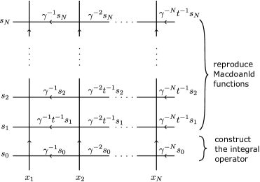
Figure 10: Operators in Proposition 4.8.

Proposition 4.8.

Let $\boldsymbol{s}^{+}=(s_{0},s_{1},\ldots,s_{N})$. Then we have

$$\bra{\boldsymbol{0}}\phi^{\mathrm{cont}}_{1,N+1}(\boldsymbol{s}^{+};x_{1})\ldots\phi^{\mathrm{cont}}_{N,N+1}(x_{N})\ket{\boldsymbol{0}}$$

$$\qquad{}=I(s_{1}/s_{0},\ldots,s_{N}/s_{0})\big{(}f^{\mathfrak{gl}_{N}}((x_{1},\ldots,x_{N});(s_{1},\ldots,s_{N})|q,q/t)\big{)}.$$

Proof.

In this proof, we put $s_{i,j}:=\gamma^{-i+1}t^{-\delta_{i>j}}s_{j}$. Here $\delta_{a>b}$ is $1$ if $a>b$ or $0$ if $a\leq b$. By taking the normal ordering, we have

$$\bra{\boldsymbol{0}}\phi^{\mathrm{cont}}_{1,N+1}(\boldsymbol{s}^{+};x_{1})\cdots\phi^{\mathrm{cont}}_{N,N+1}(x_{N})\ket{\boldsymbol{0}}$$

$$\qquad{}=\prod_{0\leq i<j\leq N}^{N}\frac{(q;q)_{\infty}(q/t;q)_{\infty}}{(\frac{qs_{j,i}}{s_{j,j}};q)_{\infty}(\frac{qs_{j,j}}{ts_{j,i}};q)_{\infty}}\prod_{1\leq i<j\leq N}\frac{(qx_{j}/tx_{i};q)_{\infty}}{(tx_{j}/x_{i};q)_{\infty}}\oint\prod_{i=1}^{N}\frac{{\rm d}y_{i,1}}{2\pi\sqrt{-1}y_{i,1}}$$

$$\qquad\phantom{=}{}\times\prod_{1\leq i<j\leq N}\frac{(qy_{j,1}/x_{i};q)_{\infty}}{(qy_{j,1}/tx_{i};q)_{\infty}}\frac{(tx_{j}/y_{i,1};q)_{\infty}}{(x_{j}/y_{i,1};q)_{\infty}}\prod_{1\leq i<j\leq N}\bigg{(}1-\frac{y_{j,1}}{y_{i,1}}\bigg{)}\frac{(qy_{j,1}/ty_{i,1};q)_{\infty}}{(ty_{j,1}/y_{i,1};q)_{\infty}}$$

$$\qquad\phantom{=}{}\times\oint\prod_{2\leq i<j\leq N}\frac{{\rm d}y_{j,i}}{2\pi\sqrt{-1}y_{j,i}}\prod_{1\leq i\leq j\leq N}\frac{(qy_{j,2}/y_{i,1};q)_{\infty}}{(qy_{j,2}/ty_{i,1};q)_{\infty}}\prod_{2\leq i<j\leq N}\frac{(ty_{j,1}/y_{i,2};q)_{\infty}}{(y_{j,1}/y_{i,2};q)_{\infty}}$$

$$\qquad\phantom{=}{}\times\bra{\boldsymbol{0}}S_{2}(y_{2,2})S_{3}(y_{3,2})S_{3}(y_{3,3})\cdots S_{N}(y_{N,2})\cdots S_{N}(y_{N,N})\ket{\boldsymbol{0}}$$

$$\qquad\phantom{=}{}\times\prod_{1\leq i<j\leq N}\frac{\theta_{q}\big{(}q\tfrac{s_{j,i}}{s_{j,j}}\tfrac{y_{j,i+1}}{y_{j,i}}\big{)}}{\theta_{q}\big{(}q\tfrac{y_{j,i+1}}{y_{j,i}}\big{)}}\prod_{i=1}^{N}\frac{\theta_{q}\big{(}q\tfrac{s_{i,0}}{s_{i,i}}\tfrac{y_{i,1}}{x_{i}}\big{)}}{\theta_{q}\big{(}q\tfrac{y_{i,1}}{x_{i}}\big{)}}.$$

As in Fact 4.5, we can rewrite the inner integrals by Macdonald functions, and we can show that

$$\prod_{1\leq i<j\leq N}^{N}\frac{(q;q)_{\infty}(q/t;q)_{\infty}}{\big{(}\frac{qs_{j,i}}{s_{j,j}};q\big{)}_{\infty}\big{(}\frac{qs_{j,j}}{ts_{j,i}};q\big{)}_{\infty}}\prod_{1\leq i<j\leq N}\frac{(qy_{j,1}/ty_{i,k};q)_{\infty}}{(qy_{j,1}/y_{i,k};q)_{\infty}}\oint\prod_{2\leq i<j\leq N}\frac{{\rm d}y_{j,i}}{2\pi\sqrt{-1}y_{j,i}}$$

$$\qquad\phantom{=}{}\times\prod_{1\leq i\leq j\leq N}\frac{(qy_{j,2}/y_{i,1};q)_{\infty}}{(qy_{j,2}/ty_{i,1};q)_{\infty}}\prod_{2\leq i<j\leq N}\frac{(ty_{j,1}/y_{i,2};q)_{\infty}}{(y_{j,1}/y_{i,2};q)_{\infty}}$$

$$\qquad\phantom{=}{}\times\bra{\boldsymbol{0}}S_{2}(y_{2,2})S_{3}(y_{3,2})S_{3}(y_{3,3})\cdots S_{N}(y_{N,2})\cdots S_{N}(y_{N,N})\ket{\boldsymbol{0}}\prod_{1\leq i<j\leq N}\frac{\theta_{q}\big{(}q\tfrac{s_{j,i}}{s_{j,j}}\tfrac{y_{j,i+1}}{y_{j,i}}\big{)}}{\theta_{q}\big{(}q\tfrac{y_{j,i+1}}{y_{j,i}}\big{)}}$$

$$\qquad{}=f^{\mathfrak{gl}_{N}}((y_{1,1},y_{2,1},\ldots,y_{N,1});(s_{1},\ldots,s_{N})|q,q/t).$$

Therefore, Proposition 4.8 follows. ∎

We prove the commutativity between the integral operator $I$ and Macdonald’s difference operator. For the proof, we need to take care of the analyticity of the domain. Hence, let us define the following region.

Notation 4.9.

Define the projection $\pi\colon(\mathbb{C}^{*})^{N}\rightarrow\mathbb{C}^{N-1}$ by

$$\pi(a_{1},\ldots,a_{N})=(a_{2}/a_{1},\ldots,a_{N}/a_{N-1}).$$

Set

$$U^{N}_{r}:=\big{\{}(z_{1},\ldots,z_{N-1})\in(\mathbb{C})^{N-1}\,|\,z_{i}<r,\ i=1,\ldots,N-1\big{\}},$$

$$B^{N}_{r}:=\big{\{}(z_{1},\ldots,z_{N-1})\in(\mathbb{C})^{N-1}\,|\,z_{i}\leq r,\ i=1,\ldots,N-1\big{\}}.$$

so that

$$\pi^{-1}\big{(}U^{N}_{r}\big{)}=\big{\{}(x_{1},\ldots,x_{N})\in(\mathbb{C}^{*})^{N};\ x_{j}/x_{i}<r^{j-i},\ 1\leq i<j\leq N\big{\}}.$$

Define the subset $\mathcal{O}(U^{N}_{r})\subset\mathbb{C}[[x_{2}/x_{1},\ldots,x_{N}/x_{N-1}]]$ to be the set of power series which absolutely convergent on the $B^{N}_{r^{\prime}}$ for any $r^{\prime}<r$, i.e., which can be regarded as a holomorphic function on $U^{N}_{r}$.

Theorem 4.10.

On $\mathcal{O}\big{(}U^{N}_{|t^{-1}|}\big{)}$, we obtain

$$[D_{x}(s_{1},\ldots,s_{N};q,q/t),\ I(s_{1}/s_{0},\ldots,s_{N}/s_{0})]=0.$$

Here, $D_{x}(\boldsymbol{s};q,t)$ is the Macdonald $q$-difference operator:

$$D_{x}(\boldsymbol{s};q,t):=\sum_{k=1}^{N}s_{k}\prod_{1\leq\ell<k}\frac{1-tx_{k}/x_{\ell}}{1-x_{k}/x_{\ell}}\prod_{k<\ell\leq n}\frac{1-x_{\ell}/tx_{k}}{1-x_{\ell}/x_{k}}T_{q,x_{k}}.$$

As for the relation between $D_{x}(\boldsymbol{s};q,t)$ and ordinary Macdonald’s difference operator, see Remark A.3. In the proof, we use the following fact.

Fact 4.11 ([27]).

It follows that

$$D_{x}\big{(}1,t^{-1},\ldots,t^{-N+1};q,t\big{)}\Pi^{(q,t)}(x|y)=D_{y^{-1}}\big{(}1,t^{-1},\ldots,t^{-N+1};q,t\big{)}\Pi^{(q,t)}(x|y).$$

Here, we put

$$D_{y^{-1}}(\boldsymbol{s};q,t):=\sum_{k=1}^{n}s_{k}\prod_{1\leq\ell<k}\frac{1-ty_{\ell}/y_{k}}{1-y_{\ell}/y_{k}}\prod_{k<\ell\leq n}\frac{1-y_{k}/ty_{\ell}}{1-y_{k}/y_{\ell}}T_{q^{-1},y_{k}}.$$

Proof of Proposition 4.10.

A direct calculation gives

$$D_{x}(\boldsymbol{s};q,q/t)\prod_{1\leq i<j\leq N}\frac{(qx_{j}/tx_{i};q)_{\infty}}{(tx_{j}/x_{i};q)_{\infty}}=\prod_{1\leq i<j\leq N}\frac{(qx_{j}/tx_{i};q)_{\infty}}{(tx_{j}/x_{i};q)_{\infty}}D_{x}(\boldsymbol{s};q,t),$$

and

$$D_{x}(\boldsymbol{s};q,t)\prod_{i=1}^{N}\frac{\theta_{q}(qs_{0}y_{i}/s_{i}x_{i})}{\theta_{q}(qy_{i}/x_{i})}\prod_{1\leq i<j\leq N}\frac{\theta_{q}(tx_{j}/y_{i})}{\theta_{q}(x_{j}/y_{i})}$$

$$\phantom{D_{x}(\boldsymbol{s};)}{}=\prod_{i=1}^{N}\frac{\theta_{q}(qs_{0}y_{i}/s_{i}x_{i})}{\theta_{q}(qy_{i}/x_{i})}\prod_{1\leq i<j\leq N}\frac{\theta_{q}(tx_{j}/y_{i})}{\theta_{q}(x_{j}/y_{i})}s_{0}D_{x}\big{(}\big{(}1,t^{-1},\ldots,t^{-N+1}\big{)};q,t\big{)}.$$

By these equations and Fact 4.11, we can show that for a function $f(x_{1},\ldots,x_{N})\in\mathcal{O}\big{(}U^{N}_{|t^{-1}|}\big{)}$,

$$D_{x}(\boldsymbol{s};q,q/t)I(s_{1}/s_{0},\ldots,s_{N}/s_{0})f(x_{1},\ldots,x_{N})$$

$$\qquad{}=\mathcal{K}(s)\prod_{1\leq i<j\leq N}\frac{(qx_{j}/tx_{i};q)_{\infty}}{(tx_{j}/x_{i};q)_{\infty}}\oint\prod_{i=1}^{N}\frac{{\rm d}y_{i}}{2\pi\sqrt{-1}y_{i}}\prod_{i=1}^{N}\frac{\theta_{q}(qs_{0}y_{i}/s_{i}x_{i})}{\theta_{q}(qy_{i}/x_{i})}$$

$$\qquad\qquad\ {}\times\prod_{1\leq i<j\leq N}\frac{\theta_{q}(tx_{j}/y_{i})}{\theta_{q}(x_{j}/y_{i})}\prod_{1\leq i<j\leq N}(1-y_{j}/y_{i})\,f(y_{1},\ldots,y_{N})s_{0}$$

$$\qquad\qquad\ {}\times D_{y^{-1}}(1,\ldots,t^{-N+1};q,t)\Pi^{(q,t)}(x|y)$$

$$\qquad{}=\mathcal{K}(s)\prod_{1\leq i<j\leq N}\frac{(qx_{j}/tx_{i};q)_{\infty}}{(tx_{j}/x_{i};q)_{\infty}}\oint\prod_{i=1}^{N}\frac{{\rm d}y_{i}}{2\pi\sqrt{-1}y_{i}}\prod_{i=1}^{N}\frac{\theta_{q}(qs_{0}y_{i}/s_{i}x_{i})}{\theta_{q}(qy_{i}/x_{i})}$$

$$\qquad\qquad\ {}\times\prod_{1\leq i<j\leq N}\frac{\theta_{q}(tx_{j}/y_{i})}{\theta_{q}(x_{j}/y_{i})}\prod_{1\leq i<j\leq N}(1-y_{j}/y_{i})\,f(y_{1},\ldots,y_{N})s_{0}$$

$$\qquad\qquad\ {}\times\sum_{k=1}^{N}\prod_{\ell\neq k}\frac{1-y_{k}/ty_{\ell}}{1-y_{k}/y_{\ell}}\,T_{q^{-1},y_{k}}\Pi^{(q,t)}(x|y).$$ (4.3)

We have poles in $y_{k}$ of the each term containing the difference operator $T_{q^{-1},y_{k}}$ at $y_{k}=q^{a}x_{k}$, $y_{k}=q^{-a}tx_{k}$, $y_{k}=q^{a+1}x_{j}$, $y_{k}=q^{-a}tx_{i}$ ($a=0,1,2,\ldots$, $i<k<j$). Therefore, by the change of variable $y_{k}\rightarrow qy_{k}$ in the each term (note that there is no pole between $y_{k}$ and $qy_{k}$), we can show that (4.3) is equal to

$$\mathcal{K}(s)\prod_{1\leq i<j\leq N}\frac{(qx_{j}/tx_{i};q)_{\infty}}{(tx_{j}/x_{i};q)_{\infty}}\oint\prod_{i=1}^{N}\frac{{\rm d}y_{i}}{2\pi\sqrt{-1}y_{i}}\,\Pi^{(q,t)}(x|y)$$

$$\qquad{}\times\sum_{k=1}^{N}t^{-k+1}T_{q,y_{k}}\prod_{1\leq\ell<k}\frac{1-ty_{\ell}/y_{k}}{1-y_{\ell}/y_{k}}\prod_{k<\ell\leq n}\frac{1-y_{k}/ty_{\ell}}{1-y_{k}/y_{\ell}}\prod_{i=1}^{N}\frac{\theta_{q}(qs_{0}y_{i}/s_{i}x_{i})}{\theta_{q}(qy_{i}/x_{i})}$$

$$\qquad{}\times\prod_{1\leq i<j\leq N}\frac{\theta_{q}(tx_{j}/y_{i})}{\theta_{q}(x_{j}/y_{i})}\prod_{1\leq i<j\leq N}(1-y_{j}/y_{i})f(y_{1},\ldots,y_{N})s_{0}$$

$$\qquad{}=\mathcal{K}(s)\prod_{1\leq i<j\leq N}\frac{(qx_{j}/tx_{i};q)_{\infty}}{(tx_{j}/x_{i};q)_{\infty}}\oint\prod_{i=1}^{N}\frac{{\rm d}y_{i}}{2\pi\sqrt{-1}y_{i}}\,\Pi^{(q,t)}(x|y)\prod_{i=1}^{N}\frac{\theta_{q}(qs_{0}y_{i}/s_{i}x_{i})}{\theta_{q}(qy_{i}/x_{i})}$$

$$\qquad\qquad\ {}\times\prod_{1\leq i<j\leq N}\frac{\theta_{q}(tx_{j}/y_{i})}{\theta_{q}(x_{j}/y_{i})}\!\!\prod_{1\leq i<j\leq N}\!\!(1-y_{j}/y_{i})D_{y}(s_{1},\ldots,s_{N}|q,q/t)f(y_{1},\ldots,y_{N}).$$

This completes the proof. ∎

Corollary 4.12.

We have

$$I(s_{1}/s_{0},\ldots,s_{N}/s_{0})\big{(}f^{\mathfrak{gl}_{N}}(x_{1},\ldots,x_{N};s_{1},\ldots,s_{N}|q,q/t)\big{)}$$

$$\qquad{}=f^{\mathfrak{gl}_{N}}(x_{1},\ldots,x_{N};s_{1},\ldots,s_{N}|q,q/t).$$

Proof.

Since by fixing $\boldsymbol{s}$, the Macdonald function $f^{\mathfrak{gl}_{N}}(\boldsymbol{x};\boldsymbol{s}|q,q/t)$ is in $\mathcal{O}\big{(}U^{N}_{|t^{-1}|}\big{)}$ (Fact A.7), we can use Theorem 4.10. Moreover, by the uniqueness of Fact A.2, we can show that $f^{\mathfrak{gl}_{N}}(\boldsymbol{x};\boldsymbol{s}|q,q/t)$ is an eigenfunction of $I(s_{1}/s_{0},\ldots,s_{N}/s_{0})$:

$$I(s_{1}/s_{0},\ldots,s_{N}/s_{0})\big{(}f^{\mathfrak{gl}_{N}}(\boldsymbol{x};\boldsymbol{s}|q,q/t)\big{)}\propto f^{\mathfrak{gl}_{N}}(\boldsymbol{x};\boldsymbol{s}|q,q/t).$$

The expansion (Proposition 4.3) makes it clear that the constant term of the LHS is $1$. Hence, the eigenvalue is $1$. ∎

4.2 Integral operator in elliptic case

In this subsection, we give brief discussion on the elliptic lift of the integral operator. Namely, consider the trace at the horizontal representation of the operator in Proposition 4.8. Then we can derive the following integral operator.

Definition 4.13.

Define the operator $I^{\mathrm{ellip}}$ on $\mathbb{C}[[x_{2}/x_{1},\ldots,x_{N}/x_{N-1}]]$ by

$$I^{\mathrm{ellip}}(s_{1}/s_{0},\ldots,s_{N}/s_{0})(f(x_{1},\ldots,x_{N}))=\left(\frac{(pq/t;q,p)_{\infty}}{(pt;q,p)_{\infty}}(p;p)\right)^{N}\mathcal{K}(\boldsymbol{s})$$

$$\qquad{}\times\prod_{1\leq i<j\leq N}\frac{\Gamma(tx_{j}/x_{i};q,p)}{\Gamma(qx_{j}/tx_{i};q,p)}\oint\prod_{i=1}^{N}\frac{{\rm d}y_{i}}{2\pi\sqrt{-1}y_{i}}\Pi^{(q,t,p)}(x|y)\prod_{i=1}^{N}\frac{\theta_{q}(qs_{0}y_{i}/s_{i}x_{i})}{\theta_{q}(qy_{i}/x_{i})}$$

$$\qquad{}\times\prod_{1\leq i<j\leq N}\frac{\theta_{q}(tx_{j}/y_{i})}{\theta_{q}(x_{j}/y_{i})}\prod_{1\leq i<j\leq N}\theta_{p}(y_{j}/y_{i})\,f(y_{1},\ldots,y_{N}).$$

Here, $\mathcal{K}(\boldsymbol{s})$ is defined in Definition 4.6. Further we set

$$\Pi^{(q,t,p)}(x|y)=\prod_{i,j=1}^{N}\frac{\Gamma(qy_{j}/tx_{i};q,p)}{\Gamma(qy_{j}/x_{i};q,p)}.$$

The following trace can be viewed as the action of $I^{\mathrm{ellip}}$ on the non-stationary Ruijsenaars functions.

Proposition 4.14.

Let $\boldsymbol{s}^{+}=(s_{0},s_{1},\ldots,s_{N})$. Then we have

$$\mathrm{tr}\big{(}p^{d}\phi^{\mathrm{cont}}_{1,N+1}(\boldsymbol{s}^{+};x_{1})\cdots\phi^{\mathrm{cont}}_{N,N+1}(x_{N})\big{)}$$

$$\qquad{}=I^{\mathrm{ellip}}(s_{1}/s_{0},\ldots,s_{N}/s_{0})\big{(}f^{\widehat{\mathfrak{gl}}_{N}}(\boldsymbol{x}^{\prime},p^{1/N}|\boldsymbol{s}^{\prime},t^{-1/N}|q,t)\big{)},$$

where we used the same notation in Theorem 3.22. As explained in Remark 4.2, we omitted the spectral parameters $\boldsymbol{s}^{+}$ in the argument of $\phi^{\mathrm{cont}}$.

Proof.

This can be proved similarly to the one of Proposition 4.8. By Lemma 3.28 and Proposition 3.29, we can show that

$$\mathrm{tr}\big{(}p^{d}\phi^{\mathrm{cont}}_{1,N+1}(\boldsymbol{s}^{+};x_{1})\cdots\phi^{\mathrm{cont}}_{N,N+1}(x_{N})\big{)}$$

$$\qquad{}=\left(\frac{(pq/t;q,p)_{\infty}}{(p;p)_{\infty}(pt;q,p)_{\infty}}\right)^{N}I^{\mathrm{ellip}}(s_{1}/s_{0},\ldots,s_{N}/s_{0})\bigg{(}\prod_{1\leq i<j\leq N}\frac{\Gamma(tx_{j}/x_{i};q,p)}{\Gamma(qx_{j}/x_{i};q,p)}$$

$$\qquad\qquad{}\times\prod_{1\leq i<j\leq N}\frac{(ts_{j}/s_{i};q)_{\infty}}{(qs_{j}/s_{i};q)_{\infty}}\,f^{\mathrm{ellip}}_{N}(\boldsymbol{s};\boldsymbol{x}|q,t,p)\bigg{)}.$$

Applying Theorem 3.30, we obtain the claim. ∎

We can obtain the commutativity between the integral operator $I^{\mathrm{ellip}}$ and the Ruijsenaars operator.

Proposition 4.15.

We obtain

$$\big{[}D_{x}(s_{1},\ldots,s_{N};q,q/t,p),I^{\mathrm{ellip}}(s_{1}/s_{0},\ldots,s_{N}/s_{0})\big{]}=0.$$

Here,

$$D_{x}(\boldsymbol{s};q,t,p):=\sum_{k=1}^{n}s_{k}\prod_{1\leq\ell<k}\frac{\theta_{p}(tx_{k}/x_{\ell})}{\theta_{p}(x_{k}/x_{\ell})}\prod_{k<\ell\leq n}\frac{\theta_{p}(x_{\ell}/tx_{k})}{\theta_{p}(x_{\ell}/x_{k})}T_{q,x_{k}}.$$

In the proof, we use the following fact.

Fact 4.16 ([37, 38]).

It follows that

$$D_{x}(1,t^{-1},\ldots,t^{-N+1};q,t,p)\Pi^{(q,t,p)}(x|y)=D_{y^{-1}}\big{(}1,t^{-1},\ldots,t^{-N+1};q,t,p\big{)}\Pi^{(q,t,p)}(x|y).$$

Here, we put

$$D_{y^{-1}}(\boldsymbol{s};q,t,p):=\sum_{k=1}^{n}s_{k}\prod_{1\leq\ell<k}\frac{\theta_{p}(ty_{\ell}/y_{k})}{\theta_{p}(y_{\ell}/y_{k})}\prod_{k<\ell\leq n}\frac{\theta_{p}(y_{k}/ty_{\ell})}{\theta_{p}(y_{k}/y_{\ell})}T_{q^{-1},y_{k}}.$$

Proof of Proposition 4.15.

A direct calculation gives

$$D_{x}(\boldsymbol{s};q,q/t,p)\prod_{1\leq i<j\leq N}\frac{\Gamma(tx_{j}/x_{i};q,p)}{\Gamma(qx_{j}/tx_{i};q,p)}=\prod_{1\leq i<j\leq N}\frac{\Gamma(tx_{j}/x_{i};q,p)}{\Gamma(qx_{j}/tx_{i};q,p)}D_{x}(\boldsymbol{s};q,t,p),$$

and

$$D_{x}(\boldsymbol{s};q,t,p)\prod_{i=1}^{N}\frac{\theta_{q}(qs_{0}y_{i}/s_{i}x_{i})}{\theta_{q}(qy_{i}/x_{i})}\prod_{1\leq i<j\leq N}\frac{\theta_{q}(tx_{j}/y_{i})}{\theta_{q}(x_{j}/y_{i})}$$

$$\qquad\qquad\,{}=\prod_{i=1}^{N}\frac{\theta_{q}(qs_{0}y_{i}/s_{i}x_{i})}{\theta_{q}(qy_{i}/x_{i})}\prod_{1\leq i<j\leq N}\frac{\theta_{q}(tx_{j}/y_{i})}{\theta_{q}(x_{j}/y_{i})}s_{0}D_{x}\big{(}\big{(}1,t^{-1},\ldots,t^{-N+1}\big{)};q,t,p\big{)}.$$

By these equations and Fact 4.16, we can show that for a function $f(x_{1},\ldots,x_{N})\in\mathcal{O}\big{(}U^{N}_{|t^{-1}|}\big{)}$,

$$D_{x}(\boldsymbol{s};q,q/t,p)I^{\mathrm{ellip}}(s_{1}/s_{0},\ldots,s_{N}/s_{0})f(x_{1},\ldots,x_{N})$$

$$\qquad{}=\left(\frac{(pq/t;q,p)_{\infty}}{(pt;q,p)_{\infty}}(p;p)\right)^{N}\mathcal{K}(s)\prod_{1\leq i<j\leq N}\frac{\Gamma(tx_{j}/x_{i};q,p)}{\Gamma(qx_{j}/tx_{i};q,p)}$$

$$\qquad\qquad{}\times\oint\prod_{i=1}^{N}\frac{{\rm d}y_{i}}{2\pi\sqrt{-1}y_{i}}\prod_{i=1}^{N}\frac{\theta_{q}(qs_{0}y_{i}/s_{i}x_{i})}{\theta_{q}(qy_{i}/x_{i})}\prod_{1\leq i<j\leq N}\frac{\theta_{q}(tx_{j}/y_{i})}{\theta_{q}(x_{j}/y_{i})}$$

$$\qquad\qquad{}\times\prod_{1\leq i<j\leq N}\theta_{p}(y_{j}/y_{i})f(y_{1},\ldots,y_{N})s_{0}D_{y^{-1}}\big{(}1,\ldots,t^{-N+1};q,t\big{)}\Pi^{(q,t)}(x|y)$$

$$\qquad{}=\left(\frac{(pq/t;q,p)_{\infty}}{(pt;q,p)_{\infty}}(p;p)\right)^{N}\mathcal{K}(s)\prod_{1\leq i<j\leq N}\frac{\Gamma(tx_{j}/x_{i};q,p)}{\Gamma(qx_{j}/tx_{i};q,p)}$$

$$\qquad\qquad{}\times\oint\prod_{i=1}^{N}\frac{{\rm d}y_{i}}{2\pi\sqrt{-1}y_{i}}\prod_{i=1}^{N}\frac{\theta_{q}(qs_{0}y_{i}/s_{i}x_{i})}{\theta_{q}(qy_{i}/x_{i})}\prod_{1\leq i<j\leq N}\frac{\theta_{q}(tx_{j}/y_{i})}{\theta_{q}(x_{j}/y_{i})}$$

$$\qquad\qquad{}\times\prod_{1\leq i<j\leq N}\theta_{p}(y_{j}/y_{i})f(y_{1},\ldots,y_{N})s_{0}\sum_{k=1}^{N}\prod_{\ell\neq k}\frac{\theta_{p}(y_{k}/ty_{\ell})}{\theta_{p}(y_{k}/y_{\ell})}\,T_{q^{-1},y_{k}}\Pi^{(q,t)}(x|y).$$ (4.4)

Similarly to the proof of Theorem 4.10, by the change of variable $y_{k}\rightarrow qy_{k}$ in the each term, we can show that (4.4) is equal to

$$\left(\frac{(pq/t;q,p)_{\infty}}{(pt;q,p)_{\infty}}(p;p)\right)^{N}\mathcal{K}(s)\prod_{1\leq i<j\leq N}\frac{\Gamma(tx_{j}/x_{i};q,p)}{\Gamma(qx_{j}/tx_{i};q,p)}\oint\prod_{i=1}^{N}\frac{{\rm d}y_{i}}{2\pi\sqrt{-1}y_{i}}\Pi^{(q,t,p)}(x|y)$$

$$\qquad{}\times\prod_{i=1}^{N}\frac{\theta_{q}(qs_{0}y_{i}/s_{i}x_{i})}{\theta_{q}(qy_{i}/x_{i})}\prod_{1\leq i<j\leq N}\frac{\theta_{q}(tx_{j}/y_{i})}{\theta_{q}(x_{j}/y_{i})}\prod_{1\leq i<j\leq N}\theta_{p}(y_{j}/y_{i})$$

$$\qquad{}\times D_{y}(s_{1},\ldots,s_{N}|q,q/t,p)f(y_{1},\ldots,y_{N}).$$

This completes the proof. ∎

In this subsection, we have derived the integral operator $I^{\mathrm{ellip}}$ and given commutativity with the Ruijsenaars operator. Unfortunately, the non-stationary Ruijsenaars functions $f^{\widehat{\mathfrak{gl}}_{N}}$ are not the eigenfunctions of the Ruijsenaars operator. So, neither for $I^{\mathrm{ellip}}$. It is left to a future study to find an operator whose eigenfunctions are $f^{\widehat{\mathfrak{gl}}_{N}}$.

5 Conformal limit $\boldsymbol{q\rightarrow 1}$

5.1 Preparation

In this section, we will derive the relation of the Virasoro algebra and the primary field from the relation of the $q$-Virasoro algebra and the Mukadé operator $\mathcal{T}^{V}$. Firstly, we define the following algebra.

Definition 5.1.

For $k=2,\dots,N$, define

$$X^{(k)}(z)=\sum_{n\in\mathbb{Z}}X^{(k)}_{n}z^{-n}=X^{(1)}\big{(}\gamma^{2(1-k)}z\big{)}X^{(1)}\big{(}\gamma^{2(2-k)}z\big{)}\cdots X^{(1)}(z)\in\mathrm{End}(\mathcal{F}_{\boldsymbol{u}})\big{[}\big{[}z^{\pm 1}\big{]}\big{]}.$$

Fact 5.2 ([5]).

The operator $X^{(k)}(z)$ is of the form

$$X^{(k)}(z)=\sum_{1\leq j_{1}<\cdots<j_{k}\leq N}{:}\Lambda^{(j_{1})}(z)\cdots\Lambda^{(j_{k})}\big{(}(q/t)^{k-1}z\big{)}{:}u_{j_{1}}\cdots u_{j_{k}}.$$

Here, $\Lambda^{(j)}(z)$ is defined in Definition 2.17.

The algebra generated by $X^{(k)}(z)$ can be regarded as the tensor product of the $q$-deformed $W_{N}$ algebra and some Heisenberg algebra [16] (See Proposition 5.20 in the next subsection). Their PBW(Poincaré–Birkhoff–Witt)-type basis is well-understood.

Definition 5.3.

For an $N$-tuple of partitions $\boldsymbol{\lambda}=\big{(}\lambda^{(1)},\lambda^{(2)},\ldots,\lambda^{(N)}\big{)}$, we define the vectors $\Ket{X_{\boldsymbol{\lambda}}}=\Ket{X_{\boldsymbol{\lambda}}(\boldsymbol{u})}\in\mathcal{F}_{\boldsymbol{u}}$ and $\Bra{X_{\boldsymbol{\lambda}}}=\Bra{X_{\boldsymbol{\lambda}}(\boldsymbol{u})}\in\mathcal{F}_{\boldsymbol{u}}^{*}$ by

$$\Ket{X_{\boldsymbol{\lambda}}(\boldsymbol{u})}:=X^{(1)}_{-\lambda^{(1)}_{1}}X^{(1)}_{-\lambda^{(1)}_{2}}\cdots X^{(2)}_{-\lambda^{(2)}_{1}}X^{(2)}_{-\lambda^{(2)}_{2}}\cdots X^{(N)}_{-\lambda^{(N)}_{1}}X^{(N)}_{-\lambda^{(N)}_{2}}\cdots\ket{\boldsymbol{0}},$$

$$\Bra{X_{\boldsymbol{\lambda}}(\boldsymbol{u})}:=\bra{\boldsymbol{0}}\cdots X^{(N)}_{\lambda^{(N)}_{2}}X^{(N)}_{\lambda^{(N)}_{1}}\cdots X^{(2)}_{\lambda^{(2)}_{2}}X^{(2)}_{\lambda^{(2)}_{1}}\cdots X^{(1)}_{\lambda^{(1)}_{2}}X^{(1)}_{\lambda^{(1)}_{1}}.$$

Fact 5.4 ([21, 33]).

The set $(\Ket{X_{\boldsymbol{\lambda}}})$ (resp. $(\Bra{X_{\boldsymbol{\lambda}}})$) form a PBW-type basis of $\mathcal{F}_{\boldsymbol{u}}$ (resp. $\mathcal{F}^{*}_{\boldsymbol{u}}$), if $u_{i}\neq q^{s}t^{-r}u_{j}$ and $u_{i}\neq 0$ for all $i,j$ and $r,s\in\mathbb{Z}$.

Definition 5.5.

Define the linear operator $\mathcal{V}(x)=\mathcal{V}\Big{(}\begin{array}[]{c}\boldsymbol{v}\\ \boldsymbol{u}\end{array};x\Big{)}\colon\mathcal{F}_{\boldsymbol{u}}\to\mathcal{F}_{\boldsymbol{v}}$ by

$$\left(1-\frac{x}{z}\right)X^{(i)}(z)\mathcal{V}(x)=\left(1-(t/q)^{i}\frac{x}{z}\right)\mathcal{V}(x)X^{(i)}(z)\qquad(i\in\{1,2,\dots,N\})$$

and the normalization condition $\bra{\boldsymbol{0}}\mathcal{V}(x)\ket{\boldsymbol{0}}=1$.

It is known that the operator $\mathcal{V}(x)$ exists uniquely [21]. Moreover, their matrix element formula is proved.

Fact 5.6 ([21]).

It follows that

$$\bra{K_{\boldsymbol{\lambda}}(\boldsymbol{v})}\mathcal{V}(x)\ket{K_{\boldsymbol{\mu}}(\boldsymbol{u})}=\frac{\big{(}(-\gamma^{2})^{N}e_{N}(\boldsymbol{u})x\big{)}^{|\boldsymbol{\lambda}|}}{(\gamma^{2}x)^{|\boldsymbol{\mu}|}}\prod_{i=1}^{N}\frac{u_{i}^{|\mu^{(i)}|}g_{\mu^{(i)}}}{\big{(}v_{i}^{|\lambda^{(i)}|}g_{\lambda^{(i)}}\big{)}^{N-1}}\prod_{i,j=1}^{N}N_{\lambda^{(i)},\mu^{(j)}}(qv_{i}/tu_{j}).$$

Remark 5.7.

The operator $\mathcal{T}^{V}(\boldsymbol{u})$ satisfies [21]

$$\left(1-\frac{w}{z}\right)X^{(i)}(z)\mathcal{T}^{V}(\boldsymbol{u},\boldsymbol{v};w)=\gamma^{-i}\left(1-\gamma^{2i}\frac{w}{z}\right)\mathcal{T}^{V}(\boldsymbol{u},\boldsymbol{v};w)X^{(i)}(z).$$

Thus, the $\mathcal{V}(x)$ can be realized by $\mathcal{T}^{V}$ with some modifications to spectral parameters.

5.2 Conformal limit $\boldsymbol{q\rightarrow 1}$

Consider the limit $q\rightarrow 1$ of $\mathcal{V}(x)=\mathcal{V}\Big{(}\begin{array}[]{c}\boldsymbol{v}\\ \boldsymbol{u}\end{array};x\Big{)}$ in the case $N=2$. Put

$$\begin{array}[]{l}q={\rm e}^{b^{-1}\hbar},\qquad t={\rm e}^{-b\hbar},\\ u_{i}={\rm e}^{u^{\prime}_{i}\hbar},\qquad v_{i}={\rm e}^{v^{\prime}_{i}\hbar}\qquad(i=1,2),\end{array}$$ (5.3)

and we parametrize $v^{\prime}_{i}$ and $u^{\prime}_{i}$ by the parameters $\mathtt{P}^{\prime}$, $\mathtt{P}$ and $\alpha$ such that

$$v^{\prime}_{i}-u^{\prime}_{j}=\mathtt{P}^{\prime}_{i}-\mathtt{P}_{j}-\alpha,\qquad i,j=1,2.$$ (5.4)

Here, we set $\mathtt{P}_{1}=-\mathtt{P}_{2}=\mathtt{P}$, $\mathtt{P}^{\prime}_{1}=-\mathtt{P}^{\prime}_{2}=\mathtt{P}^{\prime}$. Write

$$Q:=b+b^{-1}.$$

The parameters $b$, $\mathtt{P}$, $\mathtt{P}^{\prime}$, and $\alpha$ directly correspond to $b$, $P$, $P^{\prime}$, and $\alpha$ in [1], which come from the central charges of the Virasoro algebra, highest weights of its representation, and so on.

Remark 5.8.

There is an ambiguity of the choice of parametrization satisfying (5.4). No matter how we choose it, final results (Theorem 5.25) are not affected if (5.4) is satisfied. For example, the simplest parametrization is

$$u^{\prime}_{1}=\mathtt{P}+\alpha/2,\qquad u^{\prime}_{2}=-\mathtt{P}+\alpha/2,$$ (5.5)

$$v^{\prime}_{1}=\mathtt{P}^{\prime}-\alpha/2,\qquad v^{\prime}_{2}=-\mathtt{P}^{\prime}-\alpha/2.$$ (5.6)

Even if we add an arbitrary parameter to (5.5) and (5.6) to keep the degree of freedom of $u^{\prime}_{i}$ and $v^{\prime}_{i}$, the results stay the same.

It is easy to show the following lemma.

Lemma 5.9.

If (5.4) is satisfied, it follows that

$$u^{\prime}_{1}-u^{\prime}_{2}=2\mathtt{P},\qquad v^{\prime}_{1}-v^{\prime}_{2}=2\mathtt{P}^{\prime},$$

$$u^{\prime}_{1}+u^{\prime}_{2}-v^{\prime}_{1}-v^{\prime}_{2}=2\alpha.$$

The parametrization above is designed so that the following factor appears in the limit of the Nekrasov factor.

Definition 5.10.

Set

$$Z_{bif}(\alpha|\mathtt{P}^{\prime},\boldsymbol{\lambda}|\mathtt{P},\boldsymbol{\mu})=\prod_{i,j=1}^{2}\prod_{(k,l)\in\lambda^{(i)}}\big{(}\mathtt{P}^{\prime}_{i}-\mathtt{P}_{j}-\alpha+b^{-1}(a_{\lambda^{(i)}}(k,l)+1)-b\ell_{\mu^{(j)}}(k,l)\big{)}$$

$$\hphantom{Z_{bif}(\alpha|\mathtt{P}^{\prime},\boldsymbol{\lambda}|\mathtt{P},\boldsymbol{\mu})=}{}\times\prod_{(k,l)\in\mu^{(j)}}\big{(}\mathtt{P}^{\prime}_{i}-\mathtt{P}_{j}-\alpha-b^{-1}a_{\mu^{(j)}}(k,l)+b(\ell_{\lambda^{(i)}}(k,l)+1)\big{)}.$$

Proposition 5.11.

We have

$$\prod_{i,j=1}^{2}N_{\lambda^{(i)},\mu^{(i)}}(qv_{i}/tu_{j})=Z_{bif}(\alpha|\mathtt{P}^{\prime},\boldsymbol{\lambda}|\mathtt{P},\boldsymbol{\mu})\cdot\hbar^{2(|\boldsymbol{\lambda}|+|\boldsymbol{\mu}|)}+\mathcal{O}\big{(}\hbar^{2(|\boldsymbol{\lambda}|+|\boldsymbol{\mu}|)+1}\big{)}.$$

Proof.

Follows by direct calculation. ∎

Let us define bosons independent of $\hbar$ which is naturally obtained from the parameterization (5.3) and the limit $\hbar\rightarrow 0$.

Definition 5.12.

Define the Heisenberg algebra $\mathsf{a}_{n}$ ($n\in\mathbb{Z}_{\neq 0}$) by the commutation relation

$$[\mathsf{a}_{n},\mathsf{a}_{m}]=-b^{-2}n\delta_{n+m,0}.$$

Set

$$\mathsf{a}^{(1)}_{n}=\mathsf{a}_{n}\otimes 1,\qquad\mathsf{a}^{(2)}_{n}=1\otimes\mathsf{a}_{n},$$

and we assume that

$$a^{(i)}_{-n}=\mathsf{a}^{(i)}_{-n},\qquad a^{(i)}_{n}=\big{(}{-}b^{2}\big{)}\frac{1-q^{n}}{1-t^{n}}\mathsf{a}^{(i)}_{n}\qquad(n>0),$$

$$\lim_{\hbar\rightarrow 0}a^{(i)}_{-n}=\mathsf{a}^{(i)}_{-n},\qquad\lim_{\hbar\rightarrow 0}a^{(i)}_{n}=\mathsf{a}^{(i)}_{n}.$$

It is known that the generalized Macdonald functions are reduced to the generalized Jack functions [29] in the limit $\hbar\rightarrow 0$. They are defined as eigenfunctions of the following Hamiltonian. The existence theorem also follows similarly to the generalized Macdonald functions.

Definition 5.13.

Define the operator $H_{b}$ by

$$H_{b}=H_{b}^{(1)}+H_{b}^{(2)}-\big{(}1+b^{-2}\big{)}\sum_{n=1}^{\infty}n\mathsf{a}^{(1)}_{-n}\mathsf{a}^{(2)}_{n},$$

where $H_{b}^{(i)}$ ($i=1,2$) is a modified Hamiltonian of the Calogero–Sutherland model:

$$H_{b}^{(i)}\mathbin{:=}\frac{1}{2}\sum_{n,m}\left(\mathsf{a}^{(i)}_{-n}\mathsf{a}^{(i)}_{-m}\mathsf{a}^{(i)}_{n+m}+\mathsf{a}^{(i)}_{-n-m}\mathsf{a}^{(i)}_{n}\mathsf{a}^{(i)}_{m}\right)-\sum_{n=1}^{\infty}\left(b^{-1}u_{i}^{\prime}+\frac{1+b^{-2}}{2}n\right)\mathsf{a}^{(i)}_{-n}\mathsf{a}^{(i)}_{n}.$$

Fact 5.14 ([32]).

There exists a unique function $\ket{J_{\boldsymbol{\lambda}}}=\ket{J_{\boldsymbol{\lambda}}(u^{\prime}_{1},u^{\prime}_{2})}$ satisfying the following two conditions:

$$\ket{J_{\boldsymbol{\lambda}}}=\prod_{i=1}^{2}m_{\lambda^{(i)}}\big{(}\mathsf{a}^{(i)}_{-n}\big{)}\ket{\boldsymbol{0}}+\sum_{\boldsymbol{\mu}<^{\mathrm{L}}\boldsymbol{\lambda}}d_{\boldsymbol{\lambda}\boldsymbol{\mu}}\prod_{i=1}^{2}m_{\mu^{(i)}}\big{(}\mathsf{a}^{(i)}_{-n}\big{)}\ket{\boldsymbol{0}},\qquad d_{\boldsymbol{\lambda}\boldsymbol{\mu}}\in\mathbb{C};$$

$$H_{b}\ket{J_{\boldsymbol{\lambda}}}=e^{\prime}_{\boldsymbol{\lambda}}\ket{J_{\boldsymbol{\lambda}}},\qquad e^{\prime}_{\boldsymbol{\lambda}}\in\mathbb{C}.$$

Similarly, there exists a unique function $\bra{J_{\boldsymbol{\lambda}}}=\bra{J_{\boldsymbol{\lambda}}(u^{\prime}_{1},u^{\prime}_{2})}$ such that

$$\bra{J_{\boldsymbol{\lambda}}}=\bra{\boldsymbol{0}}\prod_{i=1}^{2}m_{\lambda^{(i)}}\big{(}\mathsf{a}^{(i)}_{n}\big{)}+\sum_{\boldsymbol{\mu}<^{\mathrm{R}}\boldsymbol{\lambda}}d^{\prime}_{\boldsymbol{\lambda}\boldsymbol{\mu}}\bra{\boldsymbol{0}}\prod_{i=1}^{2}m_{\mu^{(i)}}\big{(}\mathsf{a}^{(i)}_{n}\big{)},\qquad d^{\prime}_{\boldsymbol{\lambda}\boldsymbol{\mu}}\in\mathbb{C};$$

$$\bra{J_{\boldsymbol{\lambda}}}H_{b}=e^{\prime}_{\boldsymbol{\lambda}}\bra{J_{\boldsymbol{\lambda}}},\qquad e^{\prime}_{\boldsymbol{\lambda}}\in\mathbb{C}.$$

We call the eigenfunctions $\ket{J_{\boldsymbol{\lambda}}}$ and $\bra{J_{\boldsymbol{\lambda}}}$ the generalized Jack functions.

Fact 5.15 ([32]).

We have

$$\ket{P_{\boldsymbol{\lambda}}(\boldsymbol{u})}\underset{\begin{subarray}{c}\hbar\rightarrow 0,\\ u_{i}={\rm e}^{u_{i}^{\prime}\hbar},\ q={\rm e}^{b^{-1}\hbar},\ t={\rm e}^{-b\hbar}\end{subarray}}{\longrightarrow}\ket{J_{\boldsymbol{\lambda}}(u^{\prime}_{1},u^{\prime}_{2})},$$

$$\bra{P_{\boldsymbol{\lambda}}(\boldsymbol{u})}\underset{\begin{subarray}{c}\hbar\rightarrow 0,\\ {}_{i}={\rm e}^{u_{i}^{\prime}\hbar},\ q={\rm e}^{b^{-1}\hbar},\ t={\rm e}^{-b\hbar}\end{subarray}}{\longrightarrow}\bra{J_{\boldsymbol{\lambda}}(u^{\prime}_{1},u^{\prime}_{2})}.$$

In fact, the generalized Jack functions are defined for general $N$. Also for general $N$, they correspond to the limit of the generalized Macdonald function.

Next, we take the limit of the generator $X^{(i)}(z)$. In advance, we decompose the generator $X^{(i)}(z)$ into the $q$-Virasoro algebra and some Heisenberg algebra in order to obtain the relation of the Virasoro Primary fields. This decomposition can be obtained by the following linear transformation of the bosons.

Definition 5.16.

For $n>0$, define

$$b^{\prime}_{-n}:=\frac{(1-t^{-n})}{(1+(q/t)^{n})}\big{(}a^{(1)}_{-n}-\gamma^{-n}a^{(2)}_{-n}\big{)},\qquad b^{\prime}_{n}:=-\frac{(1-t^{n})}{(1+(q/t)^{n})}\big{(}a^{(1)}_{n}-\gamma^{-n}a^{(2)}_{n}\big{)},$$

$$b^{\prime\prime}_{-n}:=(1-t^{-n})\big{(}\gamma^{-2n}a^{(1)}_{-n}+\gamma^{-n}a^{(2)}_{-n}\big{)},\qquad b^{\prime\prime}_{n}:=-(1-t^{n})\big{(}a^{(1)}_{n}+\gamma^{n}a^{(2)}_{n}\big{)}.$$

Furthermore, for $n\in\mathbb{Z}_{\neq 0}$, define

$$\beta^{(1)}_{n}:=-\frac{\sqrt{-1}}{2}b\big{(}\mathsf{a}^{(1)}_{n}-\mathsf{a}^{(2)}_{n}\big{)},\qquad\beta^{(2)}_{n}:=-\frac{\sqrt{-1}}{2}b\big{(}\mathsf{a}^{(1)}_{n}+\mathsf{a}^{(2)}_{n}\big{)}.$$

Definition 5.17.

Define the zero mode by

$$\beta^{(1)}_{0}:=\sqrt{-1}\cdot\frac{u^{\prime}_{1}-u^{\prime}_{2}}{2}=\sqrt{-1}\mathtt{P},\qquad\beta^{(2)}_{0}:=\sqrt{-1}\cdot\frac{u^{\prime}_{1}+u^{\prime}_{2}}{2}\qquad\mbox{on $\mathcal{F}_{\boldsymbol{u}}$},$$

$$\beta^{(1)}_{0}:=\sqrt{-1}\cdot\frac{v^{\prime}_{1}-v^{\prime}_{2}}{2}=\sqrt{-1}\mathtt{P}^{\prime},\qquad\beta^{(2)}_{0}:=\sqrt{-1}\cdot\frac{v^{\prime}_{1}+v^{\prime}_{2}}{2}\qquad\mbox{on $\mathcal{F}_{\boldsymbol{v}}$}.$$

Proposition 5.18.

For $n,m\in\mathbb{Z}$, it follows that

$$[b^{\prime}_{n},b^{\prime}_{m}]=-n\frac{(1-q^{n})(1-t^{-n})}{(1+(q/t)^{n})}\delta_{n+m,0},$$

$$[b^{\prime}_{n},b^{\prime\prime}_{m}]=\big{[}\beta^{(1)}_{n},\beta^{(2)}_{n}\big{]}=0,$$

$$[\beta^{(2)}_{n},\beta^{(2)}_{m}]=\frac{n}{2}\delta_{n+m,0}.$$

Proof.

It follows from direct computation. ∎

Definition 5.19.

Set

$$\Lambda^{\prime}_{1}(z)={:}\exp\bigg{(}\sum_{n\neq 0}\frac{b^{\prime}_{n}}{|n|}z^{-n}\bigg{)}{:},\qquad\Lambda^{\prime}_{2}(z)={:}\exp\bigg{(}{-}\sum_{n\neq 0}\frac{b^{\prime}_{n}}{|n|}(t/q)^{n}z^{-n}\bigg{)}{:},$$

$$\Lambda^{\prime\prime}(z)=\exp\bigg{(}\sum_{n>0}\frac{b^{\prime\prime}_{-n}}{n(1+(q/t)^{n})}z^{n}\bigg{)}\exp\bigg{(}\sum_{n>0}\frac{(q/t)^{n}b^{\prime\prime}_{n}}{n(1+(q/t)^{n})}z^{-n}\bigg{)}.$$

Moreover, define

$$T(z)=\Lambda^{\prime}_{1}(z){\rm e}^{-\sqrt{-1}\hbar\beta^{(1)}_{0}}+\Lambda^{\prime}_{2}(z){\rm e}^{\sqrt{-1}\hbar\beta^{(1)}_{0}},\qquad Y(z)=\Lambda^{\prime\prime}(z){\rm e}^{-\sqrt{-1}\hbar\beta^{(2)}_{0}}.$$

Proposition 5.20.

$X^{(1)}(z)$ can be decomposed as

$$X^{(1)}(z)=T(z)Y(z).$$

Moreover we have

$$X^{(2)}(z)={:}\exp\bigg{(}\sum_{n\neq 0}\frac{b^{\prime\prime}_{n}}{|n|}z^{-n}\bigg{)}{:}{\rm e}^{-2\sqrt{-1}\hbar\beta^{(2)}_{0}}.$$

Proposition 5.21.

The operator $T(z)$ satisfies the defining relation of the $q$-Virasoro algebra:

$$f(w/z)T(z)T(w)-f(z/w)T(w)T(z)=-\frac{(1-q)\big{(}1-t^{-1}\big{)}}{1-(q/t)}(\delta(qw/tz)-\delta(tw/qz)),$$

where

$$f(z)=\exp\bigg{(}\sum_{n>0}\frac{1}{n}\frac{(1-q^{n})(1-t^{-n})}{1+(q/t)^{n}}z^{n}\bigg{)}.$$

These proposition can be shown by direct calculation. (See also [16].) For representation theory of the $q$-Virasoro algebra, we refer the reader to [45]. Now, we consider the limit of these generators.

Fact 5.22 ([45]).

The $\hbar$-expansion of $T(z)$ is of the form

$$T(z)=2-\left(L(z)-\frac{Q^{2}}{4}\right)\hbar^{2}+\mathcal{O}\big{(}\hbar^{4}\big{)}.$$

Here $L(z)=\sum_{n\in\mathbb{Z}}L_{n}z^{-n}$ is some operator written by the boson $\beta^{(1)}_{n}$. Moreover, $L_{n}$’s generate the Virasoro algebra with the central element $c=1+6Q^{2}$:

$$[L_{n},L_{m}]=(n-m)L_{n+m}+\frac{n(n-1)(n+1)c}{12}\delta_{n+m,0}.$$

Remark 5.23.

On $\mathcal{F}_{\boldsymbol{u}}^{(2,0)}$, the Virasoro algebra acts as

$$L_{0}\ket{\boldsymbol{0}}=\left(\frac{Q^{2}}{4}-\mathtt{P}^{2}\right)\ket{\boldsymbol{0}},\qquad L_{n}\ket{\boldsymbol{0}}=0\qquad(n>0).$$

Similarly, on $\mathcal{F}_{\boldsymbol{v}}^{(2,0)*}$

$$\bra{\boldsymbol{0}}L_{0}=\left(\frac{Q^{2}}{4}-\mathtt{P}^{\prime 2}\right)\bra{\boldsymbol{0}},\qquad\bra{\boldsymbol{0}}L_{-n}=0\qquad(n>0).$$

If $\mathtt{P}$, $\mathtt{P}^{\prime}$ and $b$ are generic, the following vectors form a basis on $\mathcal{F}^{(2,0)}_{\boldsymbol{u}}$ and $\mathcal{F}^{(2,0)*}_{\boldsymbol{v}}$, respectively:

$$\ket{L_{\lambda,\mu}}:=L_{-\lambda_{1}}L_{-\lambda_{2}}\cdots\beta^{(2)}_{-\mu_{1}}\beta^{(2)}_{-\mu_{2}}\cdots\ket{\boldsymbol{0}},\qquad\lambda,\mu\in\mathsf{P},$$

$$\bra{L_{\lambda,\mu}}:=\bra{\boldsymbol{0}}\cdots\beta^{(2)}_{\mu_{2}}\beta^{(2)}_{\mu_{1}}\cdots L_{\lambda_{2}}L_{\lambda_{1}},\qquad\lambda,\mu\in\mathsf{P}.$$

Hence, we can identify $\mathcal{F}_{\boldsymbol{u}}^{(2,0)}$ with the tensor product of the Verma module of the Virasoro algebra $\langle L_{n}\rangle$ and the Fock space of the Heisenberg algebra $\langle\beta^{(2)}_{n}\rangle$. Further, $\ket{\boldsymbol{0}}$ can be regarded as the tensor product of the highest wight vector of the highest weight $\frac{Q^{2}}{4}-\mathtt{P}^{2}$ and the vacuum state of the Fock space. For simplicity, we hereafter assume that $\mathtt{P}$, $\mathtt{P}^{\prime}$ and $b$ are generic so that the modules are irreducible.

By Fact 5.6, Proposition 5.11 and Fact 5.15, we can assume the following expansion. Namely, there is no pole at $\hbar=0$.

Definition 5.24.

Define $\mathcal{V}_{i}(z)$ ($i=0,1,\ldots$) to be each coefficient in the $\hbar$-expansion of $\mathcal{V}(z)=\mathcal{V}\Big{(}\begin{array}[]{c}\boldsymbol{v}\\ \boldsymbol{u}\end{array};z\Big{)}$, i.e.,

$$\mathcal{V}(z)=\mathcal{V}_{0}(z)+\mathcal{V}_{1}(z)\hbar+\mathcal{V}_{2}(z)\hbar^{2}+\cdots.$$

Furthermore, we introduce

$$\Phi^{\mathrm{H.V}}(z)=z^{-\mathtt{P}^{\prime}{}^{2}+\mathtt{P}^{2}-\alpha(Q-\alpha)}\mathcal{V}_{0}(z).$$

We obtain the result that the operator $\Phi^{\mathrm{H.V}}(z)$ corresponds to the Virasoro primary fields.

Theorem 5.25.

$\Phi^{\mathrm{H.V}}(z)$ satisfies the relation

$$[L_{n},\Phi^{\mathrm{H.V}}(z)]=z^{n}\left(z\frac{\partial}{\partial z}+\alpha(Q-\alpha)(n+1)\right)\Phi^{\mathrm{H.V}}(z).$$

Moreover, we obtain

$$\big{[}\beta^{(2)}_{n},\Phi^{\mathrm{H.V}}(w)\big{]}=\sqrt{-1}w^{n}(Q-\alpha)\Phi^{\mathrm{H.V}}(w),\qquad n>0,$$

$$\big{[}\beta^{(2)}_{-n},\Phi^{\mathrm{H.V}}(w)\big{]}=-\sqrt{-1}w^{-n}\alpha\Phi^{\mathrm{H.V}}(w),\qquad n\geq 0.$$

The proof is given in Section 5.3. Let us also state the following proposition.

Proposition 5.26.

We have

$$\frac{\braket{\widetilde{J}_{\boldsymbol{\lambda}}(v^{\prime}_{1},v^{\prime}_{2})}{\Phi^{\mathrm{H.V}}(z)}{\widetilde{J}_{\boldsymbol{\mu}}(u^{\prime}_{1},u^{\prime}_{2})}}{\bra{\boldsymbol{0}}\Phi^{\mathrm{H.V}}(z)\ket{\boldsymbol{0}}}=Z_{bif}(\alpha|p^{\prime},\boldsymbol{\lambda}|p,\boldsymbol{\mu}),$$

where we put

$$\ket{\widetilde{J}_{\boldsymbol{\lambda}}(u^{\prime}_{1},u^{\prime}_{2})}=\ket{J_{\boldsymbol{\lambda}}(u^{\prime}_{1},u^{\prime}_{2})}\lim_{\hbar\rightarrow 0}\hbar^{-N|\boldsymbol{\lambda}|}\mathcal{C}_{\boldsymbol{\lambda}}^{+}(\boldsymbol{u}),$$

$$\bra{\widetilde{J}_{\boldsymbol{\lambda}}(v^{\prime}_{1},v^{\prime}_{2})}=\bra{J_{\boldsymbol{\lambda}}(v^{\prime}_{1},v^{\prime}_{2})}\lim_{\hbar\rightarrow 0}\hbar^{-N|\boldsymbol{\lambda}|}\mathcal{C}_{\boldsymbol{\lambda}}^{-}(\boldsymbol{v}).$$

Proof.

This is clear by Fact 5.6, Fact 5.15 and Proposition 5.11. ∎

The relations in Theorem 5.25 are the exactly same as the ones in [1] up to notation. We can also check that $\ket{\widetilde{J}_{\boldsymbol{\lambda}}}$ corresponds to the Alba, Fateev, Litvinov and Tarnopolski’s (AFLT) basis [1] under the identification between the Fock space $\mathcal{F}_{\boldsymbol{u}}$ and the Verma module of the algebra $(\mathrm{Virasoro})\otimes(\mathrm{Heisemberg})$. However, $\ket{\widetilde{J}_{\boldsymbol{\lambda}}}$ and the AFLT basis are defined in the different ways. While $\ket{J_{\boldsymbol{\lambda}}}$ is defined as eigenfunctions of $H_{b}$, the AFLT basis is defined by the condition that the matrix elements of the primary fields reproduce the $Z_{bif}$. Our matrix elements formula (Fact 5.6) and Theorem 5.25 prove that $\ket{\widetilde{J}_{\vec{\lambda}}}$ and the AFLT basis actually coincide. Furthermore, these results also prove the 4D AGT correspondence [2] which states the duality between the (non-deformed) Virasoro algebra and the 4D $\mathcal{N}=2$ gauge theory. We can also expect the similar results for general $N$.

5.3 Proof of Theorem 5.25

Definition 5.27.

Define the currents

$$J^{(1)}(z)=-2\sqrt{-1}\sum_{n\in\mathbb{Z}}\beta^{(2)}_{n}z^{-n},$$

$$J^{(2)}(z)=\frac{1}{8}{:}J^{(1)}(z)^{2}{:}-\frac{1}{4}\sum_{n>0}n\big{(}\big{(}1+2b^{2}\big{)}\mathsf{a}^{(1)}_{-n}+b^{2}\mathsf{a}^{(2)}_{-n}\big{)}z^{n}$$

$$\hphantom{J^{(2)}(z)=}{}-\frac{1}{4}\sum_{n>0}n\big{(}\big{(}2+b^{2}\big{)}\mathsf{a}^{(1)}_{n}+\mathsf{a}^{(2)}_{n}\big{)}z^{-n},$$

$$\widetilde{J}^{(2)}(z)=\frac{1}{2}{:}J^{(1)}(z)^{2}{:}-\frac{1}{2}\sum_{n>0}n\big{(}\big{(}2+3b^{2}\big{)}\mathsf{a}^{(1)}_{-n}+\big{(}1+2b^{2}\big{)}\mathsf{a}^{(2)}_{-n}\big{)}z^{n}$$

$$\hphantom{\widetilde{J}^{(2)}(z)=}{}+\frac{1}{2}\sum_{n>0}n\big{(}{-}\,\mathsf{a}^{(1)}_{n}+b^{2}\mathsf{a}^{(2)}_{n}\big{)}z^{-n}.$$

These currents appear in the following expansion.

Lemma 5.28.

We have

$$Y(z)=1+\frac{1}{2}J^{(1)}(z)\hbar+J^{(2)}(z)\hbar^{2}+\mathcal{O}\big{(}\hbar^{3}\big{)},$$

$$(t/q)Y(z)=1+\left({-}Q+\frac{1}{2}J^{(1)}(z)\right)\hbar+\left(J^{(2)}(z)-\frac{1}{2}QJ^{(1)}(z)+\frac{Q^{2}}{2}\right)\hbar^{2}+\mathcal{O}\big{(}\hbar^{3}\big{)},$$

$$X^{(2)}(z)=1+J^{(1)}(z)\hbar+\widetilde{J}^{(2)}(z)\hbar^{2}+\mathcal{O}\big{(}\hbar^{3}\big{)},$$

$$(t/q)^{2}X^{(2)}(z)=1+\left({-}2Q+J^{(1)}(z)\right)\hbar+\left(\widetilde{J}^{(2)}(z)-2QJ^{(1)}(z)+2Q^{2}\right)\hbar^{2}+\mathcal{O}\big{(}\hbar^{3}\big{)}.$$

Proof.

By direct calculation. ∎

At first, we prove the relation with the Heisenberg algebra $\beta^{(2)}_{n}$.

Proposition 5.29.

We have

$$\big{[}\beta^{(2)}_{n},\mathcal{V}_{0}(w)\big{]}=\sqrt{-1}w^{n}(Q-\alpha)\mathcal{V}_{0}(w),\qquad n>0,$$ (5.7)

$$\big{[}\beta^{(2)}_{-n},\mathcal{V}_{0}(w)\big{]}=-\sqrt{-1}w^{-n}\alpha\mathcal{V}_{0}(w),\qquad n\geq 0.$$ (5.8)

Proof.

We calculate the $\hbar$-expansion of the defining relation

$$\left(X^{(2)}(z)-\frac{w}{z}X^{(2)}(z)\right)\mathcal{V}(w)=\mathcal{V}(w)\left(X^{(2)}(z)-(t/q)^{2}\frac{w}{z}X^{(2)}(z)\right).$$ (5.9)

Lemma 5.28 shows that the coefficient in front of $\hbar^{1}$ in the expansion of (5.9) is

$$\left(J^{(1)}(z)-\frac{w}{z}J^{(1)}(z)\right)\mathcal{V}_{0}(w)=\mathcal{V}_{0}(w)\left(J^{(1)}(z)-\frac{w}{z}\left({-}2Q+J^{(1)}(z)\right)\right).$$ (5.10)

The coefficients of (5.10) in front of $z^{n}$ gives the following relations.

$$\bullet z^{n} n>0$$ Coefficient of ():

$$\big{[}\beta^{(2)}_{-n},\mathcal{V}_{0}(w)\big{]}=w\big{[}\beta^{(2)}_{-n-1},\mathcal{V}_{0}(w)\big{]},$$

$$\bullet z^{0}$$ Coefficient of :

$$\big{[}\beta^{(2)}_{-1},\mathcal{V}_{0}(w)\big{]}=-\sqrt{-1}\frac{\alpha}{w}\mathcal{V}_{0}(w),$$

$$\bullet z^{-1}$$ Coefficient of :

$$\big{[}\beta^{(2)}_{1},\mathcal{V}_{0}(w)\big{]}=\sqrt{-1}w(Q-\alpha)\mathcal{V}_{0}(w),$$

$$\bullet z^{-n} n>1$$ Coefficient of ():

$$\big{[}\beta^{(2)}_{n},\mathcal{V}_{0}(w)\big{]}=w\big{[}\beta^{(2)}_{n-1},\mathcal{V}_{0}(w)\big{]}.$$

By solving inductively these relations, we can get Proposition 5.29. ∎

In the proof of Proposition 5.29, we computed the coefficient in front of $\hbar^{1}$ with respect to the relation between $\mathcal{V}(w)$ and $X^{(2)}(z)$. Actually, the same relation can be obtained from the relation between $\mathcal{V}(w)$ and $X^{(1)}(z)$. (The coefficients of $\hbar^{0}$ give trivial relations.) Next, we calculate the coefficient of $\hbar^{2}$, from which the relation with the Virasoro algebra arises. Let us introduce the following operator.

Definition 5.30.

Define $\mathcal{L}(z)=\sum_{n\in\mathbb{Z}}\mathcal{L}_{n}z^{-n}$ by

$$\mathcal{L}(z):=2J^{(2)}-\widetilde{J}^{(2)}(z)=\sum_{n,m\in\mathbb{Z}}{:}\beta^{(2)}_{n}\beta^{(2)}_{m}{:}z^{-n-m}-\sqrt{-1}Q\sum_{n\in\mathbb{Z}}n\beta^{(2)}_{n}z^{-n}.$$

Lemma 5.31.

We have

$$\left({-}L(z)+\mathcal{L}(z)-\frac{w}{z}\big{(}{-}L(z)+\mathcal{L}(z)\big{)}\right)\mathcal{V}_{0}(w)$$

$$\qquad{}=\mathcal{V}_{0}(w)\left({-}L(z)+\mathcal{L}(z)-\frac{w}{z}\big{(}{-}L(z)+\mathcal{L}(z)+QJ^{(1)}(z)-Q^{2}\big{)}\right).$$ (5.11)

Proof.

We calculate the $\hbar$-expansion of the defining relation

$$\left(1-\frac{w}{z}\right)X^{(1)}(z)\mathcal{V}(w)=\left(1-(t/q)\frac{w}{z}\right)\mathcal{V}(w)X^{(1)}(z).$$ (5.12)

By Fact 5.22 and Lemma 5.28, the coefficient of $\hbar^{2}$ in the expansion of (5.12) gives the relation

$$\left(1-\frac{w}{z}\right)\left({-}L(z)+\frac{Q^{2}}{4}+2J^{(2)}(z)\right)\mathcal{V}_{0}(w)+\left(1-\frac{w}{z}\right)J^{(1)}(z)\mathcal{V}_{1}(w)$$

$$\qquad{}=\mathcal{V}_{0}(w)\left({-}L(z)+\frac{Q^{2}}{4}+2J^{(2)}(z)-\frac{w}{z}\left({-}L(z)+\frac{Q^{2}}{4}+2J^{(2)}(z)-QJ^{(1)}(z)+Q^{2}\right)\right)$$

$$\qquad\phantom{=}{}+\mathcal{V}_{1}(w)\left(J^{(1)}(z)-\frac{w}{z}\left(J^{(1)}(z)-2Q\right)\right).$$ (5.13)

The coefficient of $\hbar^{2}$ in the $\hbar$-expansion of the defining relation (5.9) is

$$\left(1-\frac{w}{z}\right)\widetilde{J}^{(2)}(z)\mathcal{V}_{0}(z)+\left(1-\frac{w}{z}\right)J^{(1)}(z)\mathcal{V}_{1}(w)$$

$$\qquad{}=\mathcal{V}_{0}(w)\left(\widetilde{J}^{(2)}(z)-\frac{w}{z}\big{(}\widetilde{J}^{(2)}(z)-2QJ^{(1)}(z)+2Q^{2}\big{)}\right)$$

$$\qquad\phantom{=}{}+\mathcal{V}_{1}(w)\left(J^{(1)}(z)-\frac{w}{z}\big{(}J^{(1)}(z)-2Q\big{)}\right).$$ (5.14)

By subtracting (5.14) from (5.13), we can cancel the terms of $\mathcal{V}_{1}(w)$ and obtain (5.11). ∎

To obtain the relation of the Virasoro primary, we have to remove the contribution of $\mathcal{L}(z)$ from (5.11). For this purpose, we give the following lemma.

Lemma 5.32.

It follows that

$$\left(\mathcal{L}(z)-\frac{w}{z}\mathcal{L}(z)\right)\mathcal{V}_{0}(w)-\mathcal{V}_{0}(w)\left(\mathcal{L}(z)-\frac{w}{z}\big{(}\mathcal{L}(z)+QJ^{(1)}(z)-Q^{2}\big{)}\right)$$

$$\qquad{}=\alpha(Q-\alpha)\mathcal{V}_{0}(w)\sum_{n\in\mathbb{Z}}(w/z)^{n}.$$ (5.15)

Proof.

By Proposition 5.29, we can show that for $k>0$,

$$\bigg{[}\sum_{m\in\mathbb{Z}}{:}\beta^{(2)}_{k-m}\beta^{(2)}_{m}{:},\mathcal{V}_{0}(w)\bigg{]}$$

$$\qquad{}=\mathcal{V}_{0}(w)\bigg{(}{-}2\sqrt{-1}\alpha\sum_{m\geq k}\beta^{(2)}_{m}w^{k-m}+2\sqrt{-1}(Q-\alpha)\sum_{0<m<k}\beta^{(2)}_{m}w^{k-m}\bigg{)}$$

$$\qquad\phantom{=}{}-(Q-\alpha)^{2}(k-1)w^{k}\mathcal{V}_{0}(w)+2\sqrt{-1}(Q-\alpha)\sum_{m\leq 0}\beta^{(2)}_{m}w^{k-m}\mathcal{V}_{0}(w).$$

For $k=0$,

$$\bigg{[}\sum_{m\in\mathbb{Z}}{:}\beta^{(2)}_{-m}\beta^{(2)}_{m}{:},\mathcal{V}_{0}(w)\bigg{]}=-2\sqrt{-1}\alpha\mathcal{V}_{0}(w)\sum_{m>0}\beta^{(2)}_{m}w^{-m}+\alpha\left(\frac{u^{\prime}_{1}+u^{\prime}_{2}+v^{\prime}_{1}+v^{\prime}_{2}}{2}\right)\mathcal{V}_{0}(w)$$

$$\qquad{}+2\sqrt{-1}(Q-\alpha)\sum_{m>0}\beta^{(2)}_{-m}w^{m}\mathcal{V}_{0}(w).$$

For $k<0$,

$$\bigg{[}\sum_{m\in\mathbb{Z}}{:}\beta^{(2)}_{k-m}\beta^{(2)}_{m}{:},\mathcal{V}_{0}(w)\bigg{]}=-2\sqrt{-1}\alpha\mathcal{V}_{0}(w)\sum_{0\leq m}w^{k-m}\beta^{(2)}_{m}-(k+1)\alpha^{2}w^{k}\mathcal{V}_{0}(w)$$

$$\qquad{}+\bigg{(}{-}2\sqrt{-1}\alpha\sum_{k\leq m<0}w^{k-m}\beta^{(2)}_{m}+2\sqrt{-1}(Q-\alpha)\sum_{m<k}w^{k-m}\beta^{(2)}_{m}\bigg{)}\mathcal{V}_{0}(w).$$

By using these commutation relations, we can prove (5.15) at each coefficient of $z^{-k}$. ∎

By the above lemmas, we can obtain the following relation between the Virasoro algebra $L_{n}$ and $\mathcal{V}_{0}(w)$.

Proposition 5.33.

For $n\in\mathbb{Z}$, we have

$$[L_{n},\mathcal{V}_{0}(w)]=w[L_{n-1},\mathcal{V}_{0}(w)]+\alpha(Q-\alpha)w^{n}\mathcal{V}_{0}(w).$$ (5.16)

Proof.

By Lemmas 5.31 and 5.32, we have

$$\left(1-\frac{w}{z}\right)L(z)\mathcal{V}_{0}(w)-\left(1-\frac{w}{z}\right)\mathcal{V}_{0}(w)L(z)=\alpha(Q-\alpha)\mathcal{V}_{0}(w)\sum_{n\in\mathbb{Z}}(w/z)^{n}.$$

By taking the coefficient of $z^{-n}$, we get (5.16). ∎

We have proved the relations among $\mathcal{V}_{0}(w)$, the Heisenberg algebra $\beta^{(2)}_{n}$ and the Virasoro algebra $L_{n}$. Conversely, we can show that an operator satisfying these relations is unique up to the vacuum expectation value.

Lemma 5.34.

Let $\widetilde{\mathcal{V}}_{0}(w)\colon\mathcal{F}^{(2,0)}_{\boldsymbol{u}}\rightarrow\mathcal{F}^{(2,0)}_{\boldsymbol{v}}$ be an operator satisfying the relations obtained by replacing $\mathcal{V}_{0}(w)$ with $\widetilde{\mathcal{V}}_{0}(w)$ in (5.7), (5.8) and (5.16). Then, we have

$$\widetilde{\mathcal{V}}_{0}(w)=\mathcal{V}_{0}(w)\times\bra{\boldsymbol{0}}\widetilde{\mathcal{V}}_{0}(w)\ket{\boldsymbol{0}}.$$

Proof.

As we explained in Remark 5.23, we can regard $\mathcal{F}^{(2,0)}_{\boldsymbol{u}}$ and $\mathcal{F}^{(2,0)*}_{\boldsymbol{v}}$ as the modules of the Virasoro algebra $\langle L_{n}\rangle$ and the Heisenberg algebra $\langle\beta^{(2)}_{n}\rangle$. Since $\ket{L_{\lambda,\mu}}$ and $\bra{L_{\lambda,\mu}}$ form bases on $\mathcal{F}^{(2,0)}_{\boldsymbol{u}}$ and $\mathcal{F}^{(2,0)*}_{\boldsymbol{v}}$, respectively, the linear operators from $\mathcal{F}^{(2,0)}_{\boldsymbol{u}}$ to $\mathcal{F}^{(2,0)}_{\boldsymbol{v}}$ can be characterized by the matrix elements with respect to them. By (5.7), (5.8) and (5.16), the matrix elements $\braket{L_{\boldsymbol{\lambda}}}{\mathcal{V}_{0}(w)}{L_{\boldsymbol{\mu}}}$ can be attributed to the matrix elements with respect to partitions of smaller size. Indeed, if $\lambda^{(1)}\neq 0$, then (5.16) gives

$$\braket{L_{\lambda^{(1)},\lambda^{(2)}}}{\mathcal{V}_{0}(w)}{L_{\mu^{(1)},\mu^{(2)}}}=\sum_{\nu}(\mbox{const})\braket{L_{(\lambda^{(1)}-1,\lambda^{(1)}_{2},\lambda^{(1)}_{3},\ldots),\lambda^{(2)}}}{\mathcal{V}_{0}(w)}{L_{\nu,\mu^{(2)}}}.$$

Here, $\nu$ runs partitions of size $|\nu|=\big{|}\mu^{(2)}\big{|}-\big{|}\lambda^{(1)}\big{|}$ or $\big{|}\mu^{(2)}\big{|}-\big{|}\lambda^{(1)}\big{|}+1$. Eventually, there remains only the vacuum expectation value $\bra{\boldsymbol{0}}\mathcal{V}_{0}(w)\ket{\boldsymbol{0}}$ in the calculation of the matrix elements. Therefore, the operator is unique up to the vacuum expectation value. ∎

By the uniqueness of Lemma 5.34, we can prove Theorem 5.25.

Proof of Theorem 5.25.

Firstly, we prepare notations of the Verma modules and the Fock space explained in Remark 5.23. Let $M_{h_{1}}$ (resp. $M_{h_{2}}$) be the Verma module of the Virasoro algebra with the highest weight vector $\ket{h_{1}}$ (resp. $\ket{h_{2}}$) of highest weight $h_{1}=\frac{Q^{2}}{4}-\mathtt{P}^{2}$ $\big{(}$resp. $h_{2}=\frac{Q^{2}}{4}-\mathtt{P}^{\prime 2}\big{)}$. Let $F_{u}$ be the Fock space of the Heisenberg algebra $\langle\beta^{(2)}_{n}\rangle$ in which the zero mode acts as $\beta^{(2)}_{0}=u$. Then we can show that

$$\mathcal{F}_{\boldsymbol{u}}\cong M_{h_{1}}\otimes F_{u^{\prime}},\qquad u^{\prime}=\sqrt{-1}(u^{\prime}_{1}+u^{\prime}_{2})/2,$$

$$\mathcal{F}_{\boldsymbol{v}}\cong M_{h_{2}}\otimes F_{v^{\prime}},\qquad v^{\prime}=\sqrt{-1}(v^{\prime}_{1}+v^{\prime}_{2})/2$$

as representation spaces of the algebra $\langle L_{n}\rangle\otimes\langle\beta^{(2)}_{n}\rangle$. Further, let $\bra{h_{2}}$ be the dual vector such that $\bra{h_{2}}L_{0}=h_{2}\bra{h_{2}}$, $\bra{h_{2}}L_{-n}=0$ ($n>0$), and $\braket{h_{2}}{h_{2}}=1$.

Define $V^{H}(w)\colon F_{u^{\prime}}\rightarrow F_{v^{\prime}}$ by

$$V^{H}(w)=\exp\bigg{(}2\sqrt{-1}(\alpha-Q)\sum_{n>0}\frac{\beta^{(2)}_{n}}{n}w^{-n}\bigg{)}\exp\bigg{(}{-}2\sqrt{-1}\alpha\sum_{n>0}\frac{\beta^{(2)}_{-n}}{n}w^{n}\bigg{)}.$$

Then we have

$$\big{[}\beta^{(2)}_{n},V^{H}(w)\big{]}=\sqrt{-1}w^{n}(Q-\alpha)V^{H}(w),\qquad n>0,$$

$$\big{[}\beta^{(2)}_{-n},V^{H}(w)\big{]}=-\sqrt{-1}w^{-n}\alpha V^{H}(w),\qquad n\geq 0.$$

Define $V^{\rm Vir}(w)\colon M_{h_{1}}\rightarrow M_{h_{2}}$ to be the Virasoro primary field of conformal dimension $\alpha(Q-\alpha)$, i.e., it satisfies

$$\big{[}L_{n},V^{\rm Vir}(w)\big{]}=w^{n}\left(w\frac{\partial}{\partial w}+\alpha(Q-\alpha)(n+1)\right)V^{\rm Vir}(w)$$

and

$$\bra{h_{2}}V^{\rm Vir}(w)\ket{h_{1}}=w^{h_{2}-h_{1}-\alpha(Q-\alpha)}\times(\mbox{scalar}).$$

Then it follows that

$$\big{[}L_{n},V^{\rm Vir}(w)\big{]}=w\big{[}L_{n-1},V^{\rm Vir}(w)\big{]}+\alpha(Q-\alpha)w^{n}\mathcal{V}_{0}(w).$$

Therefore, Lemma 5.34 shows that

$$\Phi^{\mathrm{H.V}}(z)=V^{\rm Vir}(w)\otimes V^{H}(w)\times(\mbox{scalar})^{-1}.$$

This completes the proof. ∎

Appendix A Asymptotically free eigenfunction
of Macdonald’s difference operator

In this appendix, we briefly review basic facts of the asymptotically free eigenfunction of Macdonald’s difference operator. Consider the following modification of Macdonald’s difference operator.

Definition A.1.

Define the operator $D_{N}(\boldsymbol{s};q,t)$ on $\mathbb{Q}(q,t,\boldsymbol{s})[[x_{2}/x_{1},\ldots,x_{N}/x_{N-1}]]$ by

$$D_{N}(\boldsymbol{s};q,t):=\sum_{k=1}^{N}s_{k}\prod_{1\leq\ell<k}\frac{1-tx_{k}/x_{\ell}}{1-x_{k}/x_{\ell}}\prod_{k<\ell\leq N}\frac{1-x_{\ell}/tx_{k}}{1-x_{\ell}/x_{k}}T_{q,x_{k}},$$

where $T_{q,x_{k}}$ is the difference operator defined by

$$T_{q,x_{k}}F(x_{1},\ldots,x_{N})=F(x_{1},\ldots,qx_{k},\ldots,x_{N}).$$

An combinatorial formula for the eigenfunction of $D_{N}(\boldsymbol{s};q,t)$ was given in [11, 31, 42]. That is the function $f^{\mathfrak{gl}_{N}}$ given in Section 3.1.

Fact A.2 ([11, 31, 42]).

The function $f^{\mathfrak{gl}_{N}}(\boldsymbol{x};\boldsymbol{s}|q,t)$ is an unique formal solution to the eigenfunction equation

$$D_{N}(\boldsymbol{s};q,t)f^{\mathfrak{gl}_{N}}(\boldsymbol{x};\boldsymbol{s}|q,t)=(s_{1}+\cdots+s_{N})f^{\mathfrak{gl}_{N}}(\boldsymbol{x};\boldsymbol{s}|q,t)$$

up to scalar multiples.

Remark A.3.

The ordinary Macdonald polynomials [27] are defined as the eigenfunctions of the operator

$$\mathcal{D}_{x}=\sum_{i=1}^{N}\prod_{\begin{subarray}{c}1\leq j\leq N\\ j\neq i\end{subarray}}\frac{x_{j}-tx_{i}}{x_{j}-x_{i}}\,T_{q,x_{i}},$$

which acts on the ring of symmetric polynomials $\mathbb{Q}(q,t)[x_{1},\ldots,x_{N}]^{\mathfrak{S}_{N}}$. The eigenfunctions of this operator, that are Macdonald polynomials, are parametrized by the partitions $\lambda=(\lambda_{1},\lambda_{2},\ldots)$. By specializing $s_{i}$’s as $s_{i}=q^{\lambda_{i}}t^{N-i}$, the asymptotically free eigenfunctions $f^{\mathfrak{gl}_{N}}$ give Macdonald polynomials with partitions $\lambda$. That is to say, if $\ell(\lambda)\leq N$ and $s_{i}=q^{\lambda_{i}}t^{N-i}$, the infinite series $x^{\lambda}f^{\mathfrak{gl}_{N}}(\boldsymbol{x};\boldsymbol{s}|q,t)$ becomes a polynomial $\big{(}x^{\lambda}:=\prod_{i\geq 1}x_{i}^{\lambda_{i}}\big{)}$, and we have

$$\mathcal{D}_{x}x^{\lambda}f^{\mathfrak{gl}_{N}}(\boldsymbol{x};\boldsymbol{s}|q,t)=\sum_{i=1}^{N}q^{\lambda_{i}}t^{N-i}x^{\lambda}f^{\mathfrak{gl}_{N}}(\boldsymbol{x};\boldsymbol{s}|q,t).$$

The parameters $\boldsymbol{s}=(s_{1},\ldots,s_{n})$ and $\boldsymbol{x}=(x_{1},\ldots,x_{N})$ are symmetric to each other in the meaning of the following bispectral duality.

Fact A.4 ([31]).

It follows that

$$\prod_{1\leq i<j\leq N}\frac{(qs_{j}/s_{i};q)_{\infty}}{(qs_{j}/ts_{i};q)_{\infty}}\,f^{\mathfrak{gl}_{N}}(\boldsymbol{x};\boldsymbol{s}|q,t)=\prod_{1\leq i<j\leq N}\frac{(qx_{j}/x_{i};q)_{\infty}}{(qx_{j}/tx_{i};q)_{\infty}}\,f^{\mathfrak{gl}_{N}}(\boldsymbol{s};\boldsymbol{x}|q,t).$$

The following Poincaré duality is also important.

Fact A.5 ([31]).

It follows that

$$f^{\mathfrak{gl}_{N}}(\boldsymbol{x};\boldsymbol{s}|q,t)=\prod_{1\leq i<j\leq N}\frac{(tx_{j}/x_{i};q)_{\infty}}{(qx_{j}/tx_{i};q)_{\infty}}\,f^{\mathfrak{gl}_{N}}(\boldsymbol{x};\boldsymbol{s}|q,q/t).$$

We defined $f^{\mathfrak{gl}_{N}}(\boldsymbol{x};\boldsymbol{s}|q,t)$ as a formal power series. However, its analyticity is well-understood, and we can treat $f^{\mathfrak{gl}_{N}}(\boldsymbol{x};\boldsymbol{s}|q,t)$ as a function of several complex variables.

Notation A.6.

Define the subset $D^{N}\subset\mathbb{C}^{N-1}$ to be

$$D^{N}=\big{\{}(w_{1},\ldots,w_{N-1})\in\mathbb{C}^{N-1}\,|\,w_{i}\cdots w_{j-1}\notin q^{-\mathbb{Z}}\cup\{0\}\ (1\leq i<j\leq N)\big{\}}$$

so that

$$\pi^{-1}\big{(}D^{N}\big{)}=\big{\{}(s_{1},\ldots,s_{N})\in(\mathbb{C}^{*})^{N}\,|\,s_{j}/s_{i}\notin q^{-\mathbb{Z}}\ (1\leq i<j\leq N)\big{\}}.$$

Fact A.7 ([31]).

Let $\tau$ be a generic complex parameter. We regard $f^{\mathfrak{gl}_{N}}(\boldsymbol{x};\boldsymbol{s}|q,\tau)$ as formal power series in

$$(z_{1},\ldots,z_{N})=(x_{2}/x_{1},\ldots,x_{N}/x_{N-1}).$$

Set $r_{0}=|q/\tau|^{\frac{n-2}{n-1}}$ if $|q/\tau|\leq 1$, and $r_{0}=|\tau/q|$ if $|q/\tau|\geq 1$. Then for any $r<r_{0}$ and any compact subset $K\subset D^{N}$, the series $f^{\mathfrak{gl}_{N}}(\boldsymbol{x};\boldsymbol{s}|q,\tau)$ is absolutely convergent, uniformly on $B^{N}_{r}\times K$. Hence $f^{\mathfrak{gl}_{N}}(\boldsymbol{x};\boldsymbol{s}|q,\tau)$ defines a holomorphic function on $U^{N}_{r_{0}}\times D^{N}$. (For the notation $B^{N}_{r}$ and $U^{N}_{r}$, see Notation 4.9.)

We have the correspondence between the non-stationary Ruijsenaars functions and the ordinary Macdonald functions.

Fact A.8 ([44]).

Let $p^{\delta}\boldsymbol{x}=(p^{N/N}x_{1},\ldots,p^{1/N}x_{N})$ and $\kappa^{\delta}\boldsymbol{s}=(\kappa^{N/N}x_{1},\ldots,\kappa^{1/N}x_{N})$. Then, it follows that

$$\lim_{p\rightarrow 0}f^{\widehat{\mathfrak{gl}}_{N}}(p^{\delta}\boldsymbol{x},p|\kappa^{\delta}\boldsymbol{s},\kappa|q,t)=f^{\mathfrak{gl}_{N}}(\boldsymbol{x};\boldsymbol{s}|q,q/t).$$

By this limit, we can check that Theorem 3.22 is certainly consistent with Fact 3.13.

Appendix B Non-stationary Ruijsenaars functions
and affine screening current

We recall the screening currents and vertex operators depending on the parameter $\kappa$. The operators in the main text correspond to the specialized case $\kappa\rightarrow t^{-1}$.

Definition B.1.

Let $S_{i}(z),\phi_{i}(z)\in\widehat{\mathcal{H}}^{N}[z]$ be operators satisfying

$$S_{i}(z)S_{i}(w)={(w/z;q)_{\infty}\over(tw/z;q)_{\infty}}{(qw/tz;q)_{\infty}\over(qw/z;q)_{\infty}}{:}S_{i}(z)S_{i}(w){:},$$

$$S_{i}(z)S_{i+1}(w)={\big{(}\kappa^{1/N}qw/z;q\big{)}_{\infty}\over\big{(}\kappa^{1/N}qw/tz;q\big{)}_{\infty}}{:}S_{i}(z)S_{i+1}(w){:},$$

$$S_{i+1}(z)S_{i}(w)={\big{(}\kappa^{-1/N}tw/z;q\big{)}_{\infty}\over\big{(}\kappa^{-1/N}w/z;q\big{)}_{\infty}}{:}S_{i+1}(z)S_{i}(w){:},$$

$$\phi_{i}(z)\phi_{i}(w)={(w/z;q,\kappa)_{\infty}\over(tw/z;q,\kappa)_{\infty}}{(\kappa qw/z;q,\kappa)_{\infty}\over(\kappa qw/tz;q,\kappa)_{\infty}}{:}\phi_{i}(z)\phi_{i}(w){:}\qquad(0\leq i\leq N-1),$$

$$\phi_{i}(z)\phi_{j}(w)={\big{(}\kappa^{(-i+j)/N}w/z;q,\kappa\big{)}_{\infty}\over\big{(}\kappa^{(-i+j)/N}tw/z;q,\kappa\big{)}_{\infty}}{\big{(}\kappa^{(-i+j)/N}qw/z;q,\kappa\big{)}_{\infty}\over\big{(}\kappa^{(-i+j)/N}qw/tz;q,\kappa\big{)}_{\infty}}{:}\phi_{i}(z)\phi_{j}(w){:}$$

$$\hphantom{\phi_{i}(z)\phi_{j}(w)=}(0\leq i<j\leq N-1),$$

$$\phi_{i}(z)\phi_{j}(w)={\big{(}\kappa^{(-i+j+N)/N}w/z;q,\kappa\big{)}_{\infty}\over\big{(}\kappa^{(-i+j+N)/N}tw/z;q,\kappa\big{)}_{\infty}}{\big{(}\kappa^{(-i+j+N)/N}qw/z;q,\kappa\big{)}_{\infty}\over\big{(}\kappa^{(-i+j+N)/N}qw/tz;q,\kappa\big{)}_{\infty}}{:}\phi_{i}(z)\phi_{j}(w){:}$$

$$\hphantom{\phi_{i}(z)\phi_{j}(w)=}(0\leq j<i\leq N-1),$$

and

$$\phi_{i}(z)S_{i+1}(w)={\big{(}\kappa^{1/N}qw/z;q\big{)}_{\infty}\over\big{(}\kappa^{1/N}qw/tz;q\big{)}_{\infty}}{:}\phi_{i}(z)S_{i+1}(w){:},$$

$$S_{i+1}(w)\phi_{i}(z)={\big{(}\kappa^{-1/N}tz/w;q\big{)}_{\infty}\over\big{(}\kappa^{-1/N}z/w;q\big{)}_{\infty}}{:}\phi_{i}(z)S_{i+1}(w){:},$$

$$\phi_{i}(z)S_{i}(w)={(w/z;q)_{\infty}\over(tw/z;q)_{\infty}}{:}\phi_{i}(z)S_{i}(w){:},\qquad S_{i}(w)\phi_{i}(z)={(qz/tw;q)_{\infty}\over(qz/w;q)_{\infty}}{:}\phi_{i}(z)S_{i}(w){:},$$

$$\phi_{i}(z)S_{j}(w)={:}\phi_{i}(z)S_{j}(w){:},\qquad S_{j}(w)\phi_{i}(z)={:}\phi_{i}(z)S_{j}(w){:}\qquad(j\neq i,i+1).$$

The screened vertex operator having the parameter $\kappa$ is defined as follows.

Definition B.2.

For $1\leq i\leq N-1$ and $\lambda\in\mathsf{P}$, define

$$\phi^{i}_{\lambda}(z)=\phi_{i-\ell}(\kappa^{(\ell+1)/N}z)\prod^{\curvearrowleft}_{1\leq j\leq\ell}S_{i-j+1}\big{(}\kappa^{j/N}q^{\lambda_{j}}z\big{)},$$

$$\Phi^{i}_{\lambda}(z)=\left({(q/t;q)_{\infty}\over(q;q)_{\infty}}\right)^{\ell(\lambda)}\phi^{i}_{\lambda}(z),$$

$$\Phi^{i}(z|x,p)=\sum_{\lambda\in\mathsf{P}}\Phi^{i}_{\lambda}(z)\prod_{k\geq 1}\big{(}p^{1/N}x_{N-i+k}/x_{N-i+k-1}\big{)}^{\lambda_{k}}.$$

Notation B.3.

For $1\leq i\leq N$, set

$$\omega^{i}=(\omega^{i}_{1},\ldots,\omega^{i}_{N})=(\overbrace{0,\ldots,0}^{i\ {\rm times}},1,\ldots,1)\in\mathbb{Z}^{N}.$$

We write

$$t^{\omega^{i}}x=\big{(}t^{\omega^{i}_{1}}x_{1},\ldots,t^{\omega^{i}_{N}}x_{N}\big{)}.$$

The non-stationary Ruijsenaars functions can be constructed by the screened vertex operators.

Fact B.4 ([44]).

Let $N\in\mathbb{Z}_{\geq 2}$. Then, it follows that

$$\langle 0|\Phi^{0}\big{(}1/s_{N}|t^{\omega^{N}}x,p\big{)}\Phi^{1}\big{(}1/s_{N-1}|t^{\omega^{N-1}}x,p\big{)}\cdots\Phi^{N-1}\big{(}1/s_{1}|t^{\omega^{1}}x,p\big{)}|0\rangle$$

$$\qquad{}=\sum_{\lambda^{(1)},\ldots,\lambda^{(N)}\in\mathsf{P}}\langle 0|\Phi^{0}_{\lambda^{(N)}}(1/s_{N})\Phi^{1}_{\lambda^{(N-1)}}(1/s_{N-1})\cdots\Phi^{N-1}_{\lambda^{(1)}}(1/s_{1})|0\rangle$$

$$\qquad\qquad{}\times\mathfrak{t}(\boldsymbol{\lambda})\prod_{j=1}^{N}\prod_{i\geq 1}(p^{1/N}x_{j+i}/x_{j+i-1})^{\lambda^{(j)}_{i}}$$

$$\qquad{}=\prod_{1\leq i<j\leq N}{(\kappa^{(j-i)/N}s_{j}/s_{i};q,\kappa)_{\infty}\over(\kappa^{(j-i)/N}ts_{j}/s_{i};q,\kappa)_{\infty}}{(\kappa^{(j-i)/N}qs_{j}/s_{i};q,\kappa)_{\infty}\over(\kappa^{(j-i)/N}qs_{j}/ts_{i};q,\kappa)_{\infty}}f^{\widehat{\mathfrak{g}l}_{N}}\big{(}x,p^{1/N}|s,\kappa^{1/N}|q,t\big{)}.$$

Here, we put

$$\mathfrak{t}(\boldsymbol{\lambda}):=\prod_{i=1}^{N}t^{-|\lambda^{(i)}|+|\lambda^{(i)}|^{(0)}}\prod_{0\leq i<j\leq N-1}t^{|\lambda^{(N-i)}|^{(N+i-j)}+|\lambda^{(N-j)}|^{(-i+j-1)}}$$

$$\hphantom{\mathfrak{t}(\boldsymbol{\lambda}):}=\prod_{i=1}^{N}t^{-|\lambda^{(i)}|^{(i-1)}+|\lambda^{(i)}|^{(0)}}.$$

Note that there is a typo in [44], and the corresponding formula Theorem 2.13 in [44] should be read as in Fact B.4.

Appendix C Some combinatorial formulas

C.1 Proof of Lemma 3.19

By using factorials, we can rewrite the Nekrasov factors as follows. If $k\neq i$,

$$N_{\mu^{(k-1)},\mu^{(k)}}(Q)$$

$$\qquad{}=\prod_{\begin{subarray}{c}h\equiv i-k\\ j-h\equiv 0\\ j\geq h\geq 1\end{subarray}}\!\!\big{(}Qq^{-\lambda_{h}+\lambda_{j+N+1}}t^{\frac{h-j}{N}};q\big{)}_{\lambda_{j+1}-\lambda_{j+N+1}}\prod_{\begin{subarray}{c}h\equiv i-k+1\\ j-h\equiv 0\\ j\geq h\geq 1\end{subarray}}\!\!\big{(}Qq^{\lambda_{h}-\lambda_{j-1}}t^{\frac{j-h}{N}+1};q\big{)}_{\lambda_{j-1}-\lambda_{j+N-1}}.$$

Decomposing factors which will be canceled afterward, we have

$$N_{\mu^{(k-1)},\mu^{(k)}}(Q)=A^{(k-1,k)}(Q)\cdot\widetilde{A}^{(k-1,k)}(Q)\qquad(k\neq i),$$

where we put

$$A^{(k-1,k)}(Q):=\prod_{\begin{subarray}{c}h\equiv i-k\\ j-h\equiv 0\\ j\geq h\geq 1\end{subarray}}\big{(}Qq^{-\lambda_{h}+\lambda_{j+N}}t^{\frac{h-j}{N}};q\big{)}_{\lambda_{j+1}-\lambda_{j+N}}\prod_{\begin{subarray}{c}h\equiv i-k+1\\ j-h\equiv 0\\ j\geq h\geq 1\end{subarray}}\big{(}Qq^{\lambda_{h}-\lambda_{j}}t^{\frac{j-h}{N}+1};q\big{)}_{\lambda_{j}-\lambda_{j+N-1}},$$

$$\widetilde{A}^{(k-1,k)}(Q):=\!\prod_{\begin{subarray}{c}h\equiv i-k\\ j-h\equiv 0\\ j\geq h\geq 1\end{subarray}}\!\!\big{(}Qq^{-\lambda_{h}+\lambda_{j+N+1}}t^{\frac{h-j}{N}};q\big{)}_{\lambda_{j+N}-\lambda_{j+N+1}}\!\!\!\prod_{\begin{subarray}{c}h\equiv i-k+1\\ j-h\equiv 0\\ j\geq h\geq 1\end{subarray}}\!\!\!\!\big{(}Qq^{\lambda_{h}-\lambda_{j-1}}t^{\frac{j-h}{N}+1};q\big{)}_{\lambda_{j-1}-\lambda_{j}}.$$

Similarly, we have

$$N_{\mu^{(i-1)},\mu^{(i)}}(Q)=\prod_{\begin{subarray}{c}h\equiv N\\ j-h\equiv 0\\ j\geq h\geq 1\end{subarray}}\big{(}Qq^{-\lambda_{h}+\lambda_{j+1}}t^{\frac{h-j}{N}};q\big{)}_{\lambda_{j-N+1}-\lambda_{j+1}}\!\!\prod_{\begin{subarray}{c}\alpha\equiv 1\\ \beta-\alpha\equiv-1\\ \beta\geq\alpha\geq 1\end{subarray}}\!\!\big{(}Qq^{\lambda_{\alpha}-\lambda_{\beta}}t^{\frac{\beta-\alpha+1}{N}};q\big{)}_{\lambda_{\beta}-\lambda_{\beta+N}}\$$

$$\hphantom{N_{\mu^{(i-1)},\mu^{(i)}}(Q)}{}=A^{(i-1,i)}(Q)\cdot\widetilde{A}^{(i-1,i)}(Q),$$

where we put

$$A^{(i-1,i)}(Q):=\prod_{\begin{subarray}{c}h\equiv N\\ j-h\equiv 0\\ j\geq h\geq 1\end{subarray}}\big{(}Qq^{-\lambda_{h}+\lambda_{j}}t^{\frac{h-j}{N}};q\big{)}_{\lambda_{j-N+1}-\lambda_{j}}\prod_{\begin{subarray}{c}\alpha\equiv 1\\ \beta-\alpha\equiv-1\\ \beta\geq\alpha\geq 1\end{subarray}}\big{(}Qq^{\lambda_{\alpha}-\lambda_{\beta+1}}t^{\frac{\beta-\alpha+1}{N}};q\big{)}_{\lambda_{\beta+1}-\lambda_{\beta+N}},$$

$$\widetilde{A}^{(i-1,i)}(Q):=\prod_{\begin{subarray}{c}h\equiv N\\ j-h\equiv 0\\ j\geq h\geq 1\end{subarray}}\big{(}Qq^{-\lambda_{h}+\lambda_{j+1}}t^{\frac{h-j}{N}};q\big{)}_{\lambda_{j}-\lambda_{j+1}}\prod_{\begin{subarray}{c}\alpha\equiv 1\\ \beta-\alpha\equiv-1\\ \beta\geq\alpha\geq 1\end{subarray}}\big{(}Qq^{\lambda_{\alpha}-\lambda_{\beta}}t^{\frac{\beta-\alpha+1}{N}};q\big{)}_{\lambda_{\beta}-\lambda_{\beta+1}}.$$

For $k=1,\ldots,N$,

$$N_{\mu^{(k)},\mu^{(k)}}(Q)=\prod_{\begin{subarray}{c}h\equiv i-k\\ j-h\equiv 0\\ j\geq h\geq 1\end{subarray}}\big{(}Qq^{-\lambda_{h}+\lambda_{j+N}}t^{\frac{h-j}{N}};q\big{)}_{\lambda_{j}-\lambda_{j+N}}\prod_{\begin{subarray}{c}h\equiv i-k\\ j-h\equiv 0\\ j\geq h\geq 1\end{subarray}}\big{(}Qq^{\lambda_{h}-\lambda_{j}}t^{\frac{j-h}{N}+1};q\big{)}_{\lambda_{j}-\lambda_{j+N}}$$

$$\hphantom{N_{\mu^{(k)},\mu^{(k)}}(Q)}{}=B^{(k)}(Q)\cdot\widetilde{B}^{(k)}(Q),$$

where we put

$$B^{(k)}(Q):=\prod_{\begin{subarray}{c}h\equiv i-k\\ j-h\equiv 0\\ j\geq h\geq 1\end{subarray}}\big{(}Qq^{-\lambda_{h}+\lambda_{j+N}}t^{\frac{h-j}{N}};q\big{)}_{\lambda_{j+1}-\lambda_{j+N}}\prod_{\begin{subarray}{c}h\equiv i-k\\ j-h\equiv 0\\ j\geq h\geq 1\end{subarray}}\big{(}Qq^{\lambda_{h}-\lambda_{j}}t^{\frac{j-h}{N}+1};q\big{)}_{\lambda_{j}-\lambda_{j+N-1}},$$

$$\widetilde{B}^{(k)}(Q):=\prod_{\begin{subarray}{c}h\equiv i-k\\ j-h\equiv 0\\ j\geq h\geq 1\end{subarray}}\big{(}Qq^{-\lambda_{h}+\lambda_{j+1}}t^{\frac{h-j}{N}};q\big{)}_{\lambda_{j}-\lambda_{j+1}}\prod_{\begin{subarray}{c}h\equiv i-k\\ j-h\equiv 0\\ j\geq h\geq 1\end{subarray}}\big{(}Qq^{\lambda_{h}-\lambda_{j+N-1}}t^{\frac{j-h}{N}+1};q\big{)}_{\lambda_{j+N-1}-\lambda_{j+N}}.$$

Then, it is clear that

$$\prod_{1\leq k\leq N}\widetilde{B}^{(k)}(1)=\mathsf{N}^{(0)}_{\lambda\lambda}\big{(}1|q,t^{-1/N}\big{)}.$$

Since it follows that

$$A^{(i-1,i)}(Q)=\prod_{\begin{subarray}{c}h\equiv N\\ j-h\equiv 0\\ j\geq h\geq 1\end{subarray}}\big{(}Qq^{-\lambda_{h}+\lambda_{j+N}}t^{\frac{h-j}{N}-1};q\big{)}_{\lambda_{j+1}-\lambda_{j+N}}\prod_{\begin{subarray}{c}h\equiv N\\ h\geq 1\end{subarray}}(Q;q)_{\lambda_{h-N+1}-\lambda_{h}}$$

$$\hphantom{A^{(i-1,i)}(Q)=}{}\times\prod_{\begin{subarray}{c}\alpha\equiv 1\\ \beta-\alpha\equiv-1\\ \beta\geq\alpha\geq 1\end{subarray}}\big{(}Qq^{\lambda_{\alpha}-\lambda_{\beta+1}}t^{\frac{\beta-\alpha+1}{N}};q\big{)}_{\lambda_{\beta+1}-\lambda_{\beta+N}}$$

$$\hphantom{A^{(i-1,i)}(Q)}{}=\prod_{\begin{subarray}{c}h\equiv N\\ j-h\equiv 0\\ j\geq h\geq 1\end{subarray}}\big{(}Qq^{-\lambda_{h}+\lambda_{j+N}}t^{\frac{h-j}{N}-1};q\big{)}_{\lambda_{j+1}-\lambda_{j+N}}\prod_{\begin{subarray}{c}\alpha\equiv 1\\ \beta-\alpha\equiv 0\\ \beta\geq\alpha\geq 1\end{subarray}}\big{(}Qq^{\lambda_{\alpha}-\lambda_{\beta}}t^{\frac{\beta-\alpha}{N}};q\big{)}_{\lambda_{\beta}-\lambda_{\beta+N-1}},$$

we have

$$\prod_{1\leq k\leq N}\frac{A^{(k-1,k)}(t^{\delta_{k,i}})}{B^{(k)}(1)}=1.$$

By the above computation, it follows that

$$\prod_{1\leq k\leq N}\frac{N_{\mu^{(k-1)},\mu^{(k)}}(t^{\delta_{k,i}})}{N_{\mu^{(k)},\mu^{(k)}}(1)}=\frac{1}{\mathsf{N}^{(0)}_{\lambda\lambda}(1|q,t^{-1/N})}\,\widetilde{A}^{(i-1,i)}(t)\prod_{k\neq i}\widetilde{A}^{(k-1,k)}(1).$$

Furthermore, it can be shown that for $k\neq i$,

$$\widetilde{A}^{(k-1,k)}(1)=\prod_{\begin{subarray}{c}h\equiv i-k\\ j-h\equiv 0\\ j\geq h\geq 1\end{subarray}}\big{(}q^{-\lambda_{h}+\lambda_{j+N+1}}t^{\frac{h-j}{N}};q\big{)}_{\lambda_{j+N}-\lambda_{j+N+1}}$$

$$\phantom{\widetilde{A}^{(k-1,k)}(1)=}{}\times\prod_{\begin{subarray}{c}h\equiv i-k+1\\ j-h\equiv 0\\ j\geq h\geq 1\end{subarray}}\big{(}q^{\lambda_{h}-\lambda_{j+N-1}}t^{\frac{j-h}{N}+2};q\big{)}_{\lambda_{j+N-1}-\lambda_{j+N}}\prod_{\begin{subarray}{c}h\equiv i-k+1\\ h\geq 1\end{subarray}}\big{(}q^{\lambda_{h}-\lambda_{h-1}}t;q\big{)}_{\lambda_{h-1}-\lambda_{h}}$$

$$\phantom{\widetilde{A}^{(k-1,k)}(1)}{}=\prod_{\begin{subarray}{c}h\equiv i-k\\ j-h\equiv 0\\ j\geq h\geq 1\end{subarray}}\big{(}q^{-\lambda_{h}+\lambda_{j+1}}t^{\frac{h-j}{N}+1};q\big{)}_{\lambda_{j}-\lambda_{j+1}}\prod_{\begin{subarray}{c}\alpha\equiv i-k+1\\ \beta-\alpha\equiv-1\\ \beta\geq\alpha\geq 1\end{subarray}}\big{(}q^{\lambda_{\alpha}-\lambda_{\beta}}t^{\frac{\beta-\alpha+1}{N}+1};q\big{)}_{\lambda_{\beta}-\lambda_{\beta+1}}.$$

Therefore, we obtain

$$\prod_{1\leq k\leq N}\frac{N_{\mu^{(k-1)},\mu^{(k)}}(t^{\delta_{k,i}})}{N_{\mu^{(k)},\mu^{(k)}}(1)}=\frac{\mathsf{N}^{(0)}_{\lambda\lambda}(t|q,t^{-1/N})}{\mathsf{N}^{(0)}_{\lambda\lambda}(1|q,t^{-1/N})}.$$

C.2 Proof of Theorem 2.24

By Fact 3.35, we have

$$\bra{P_{\boldsymbol{\lambda}}(\boldsymbol{v})}\mathcal{T}^{V}(\boldsymbol{u},\boldsymbol{v},w)\ket{Q_{\boldsymbol{\mu}}(\boldsymbol{u})}$$

$$\qquad{}=\zeta^{\sharp}\times\frac{\prod_{i,j=1}^{N}N_{\lambda^{(i)},\mu^{(j)}}(v_{i}/\gamma u_{j})}{\prod_{k=1}^{N}c_{\lambda^{(k)}}c^{\prime}_{\mu^{(k)}}\prod_{1\leq i<j\leq N}N_{\mu^{(i)},\mu^{(j)}}(qu_{i}/tu_{j})\prod_{1\leq i<j\leq N}N_{\lambda^{(j)},\lambda^{(i)}}(qv_{j}/tv_{i})},$$

where

$$\zeta^{\sharp}:=\mathcal{M}(\boldsymbol{u},\boldsymbol{v};\boldsymbol{\lambda},\boldsymbol{\mu};w)\cdot\xi^{(+)}_{\boldsymbol{\mu}}(\boldsymbol{u})^{-1}\cdot\xi^{(-)}_{\boldsymbol{\lambda}}(\boldsymbol{v})^{-1}.$$

On the other hand, by using the relation

$$N_{\lambda,\mu}(\gamma^{-1}x)=N_{\mu,\lambda}(\gamma^{-1}x^{-1})x^{|\lambda|+|\mu|}\frac{f_{\lambda}}{f_{\mu}},$$

we have

$$\bra{\boldsymbol{\mu}}\mathcal{T}^{H}(\boldsymbol{u},\boldsymbol{v};w)\ket{\boldsymbol{\lambda}}$$

$$\qquad{}=\zeta^{\flat}\times\frac{\prod_{i,j=1}^{N}N_{\lambda^{(i)},\mu^{(j)}}(v_{i}/\gamma u_{j})}{\prod_{k=1}^{N}c_{\lambda^{(k)}}c^{\prime}_{\mu^{(k)}}\prod_{1\leq i<j\leq N}N_{\mu^{(i)},\mu^{(j)}}(qu_{i}/tu_{j})\prod_{1\leq i<j\leq N}N_{\lambda^{(j)},\lambda^{(i)}}(qv_{j}/tv_{i})},$$

where

$$\zeta^{\flat}:=\prod_{i=1}^{N}\hat{t}\big{(}\lambda^{(i)},\tfrac{u_{1}\cdots u_{i}}{v_{1}\cdots v_{i}}w,v_{i},0\big{)}c_{\lambda^{(i)}}\hat{t}^{*}\big{(}\mu^{(i)},u_{i},\tfrac{u_{1}\cdots u_{i-1}}{v_{1}\cdots v_{i-1}}w,0\big{)}c^{\prime}_{\mu^{(i)}}$$

$$\hphantom{\zeta^{\flat}:=}{}\times\prod_{1\leq i<j\leq N}(\gamma u_{j}/u_{i})^{-|\mu^{(i)}|-|\mu^{(j)}|}\frac{f_{\mu^{(i)}}}{f_{\mu^{(j)}}}\prod_{1\leq i<j\leq N}(u_{j}/u_{i})^{|\lambda^{(i)}|+|\mu^{(j)}|}\frac{f_{\mu^{(j)}}}{f_{\lambda^{(i)}}}.$$

A direct calculation gives

$$\zeta^{\sharp}=w^{|\boldsymbol{\lambda}|-|\boldsymbol{\mu}|}(-1)^{N|\boldsymbol{\lambda}|+(N+1)|\boldsymbol{\mu}|}\gamma^{(N+1)|\boldsymbol{\lambda}|+(-2N+1)|\boldsymbol{\mu}|}e_{N}(\boldsymbol{u})^{|\boldsymbol{\lambda}|}$$

$$\phantom{\zeta^{\sharp}=}{}\times\prod_{i=1}^{N}q^{n(\mu^{(i)^{\prime}})+n(\lambda^{(i)^{\prime}})+|\mu^{(i)}|}g_{\lambda^{(i)}}^{-N+i-1}g_{\mu^{(i)}}^{N-i}(-1)^{i|\lambda^{(i)}|+i|\mu^{(i)}|}\gamma^{-i|\lambda^{(i)}|+i|\mu^{(i)}|}$$

$$\phantom{\zeta^{\sharp}=}{}\times\prod_{i=1}^{N}u_{i}^{(N-i+1)|\mu^{(i)}|-\sum_{k=1}^{i}|\mu^{(k)}|}\times\prod_{i=1}^{N}v_{i}^{(i-N)|\lambda^{(i)}|-\sum_{k=i}^{N}|\lambda^{(k)}|}=(-1)^{|\boldsymbol{\lambda}|+|\boldsymbol{\mu}|}\zeta^{\flat}.$$

This completes the proof of Theorem 2.24.

Acknowledgments

The authors would like to thank H. Awata, B. Feigin, A. Hoshino, H. Kanno, Y. Matsuo, M. Noumi and S. Yanagida for valuable comments. The authors are also grateful to the referees for helpful feedback. The research of J.S. is supported by JSPS KAKENHI (Grant Numbers 19K03512). Y.O. and M.F. are partially supported by Grant-in-Aid for JSPS Research Fellow (Y.O.: 18J00754, M.F.: 17J02745).

References

- [1] Alba V.A., Fateev V.A., Litvinov A.V., Tarnopolskiy G.M., On combinatorial expansion of the conformal blocks arising from AGT conjecture, Lett. Math. Phys. 98 (2011), 33–64, arXiv:1012.1312.
- [2] Alday L.F., Gaiotto D., Tachikawa Y., Liouville correlation functions from four-dimensional gauge theories, Lett. Math. Phys. 91 (2010), 167–197, arXiv:0906.3219.
- [3] Atai F., Langmann E., Series solutions of the non-stationary Heun equation, SIGMA 14 (2018), 011, 32 pages, arXiv:1609.02525.
- [4] Atai F., Langmann E., Exact solutions by integrals of the non-stationary elliptic Calogero–Sutherland equation, J. Integrable Syst. 5 (2020), xyaa001, 26 pages, arXiv:1908.00529.
- [5] Awata H., Feigin B., Hoshino A., Kanai M., Shiraishi J., Yanagida S., Notes on Ding–Iohara algebra and AGT conjecture, RIMS Kōkyūroku 1765 (2011), 12–32, arXiv:1106.4088.
- [6] Awata H., Feigin B., Shiraishi J., Quantum algebraic approach to refined topological vertex, J. High Energy Phys. 2012 (2012), no. 3, 041, 35 pages, arXiv:1112.6074.
- [7] Awata H., Fujino H., Ohkubo Y., Crystallization of deformed Virasoro algebra, Ding–Iohara–Miki algebra, and 5D AGT correspondence, J. Math. Phys. 58 (2017), 071704, 25 pages, arXiv:1512.08016.
- [8] Awata H., Kanno H., Refined BPS state counting from Nekrasov’s formula and Macdonald functions, Internat. J. Modern Phys. A 24 (2009), 2253–2306, arXiv:0805.0191.
- [9] Awata H., Kanno H., Changing the preferred direction of the refined topological vertex, J. Geom. Phys. 64 (2013), 91–110, arXiv:0903.5383.
- [10] Awata H., Matsuo Y., Odake S., Shiraishi J., Collective field theory, Calogero–Sutherland model and generalized matrix models, Phys. Lett. B 347 (1995), 49–55, arXiv:hep-th/9411053.
- [11] Braverman A., Finkelberg M., Shiraishi J., Macdonald polynomials, Laumon spaces and perverse coherent sheaves, in Perspectives in Representation Theory, Contemp. Math., Vol. 610, Amer. Math. Soc., Providence, RI, 2014, 23–41, arXiv:1206.3131.
- [12] Carlsson E., Nekrasov N., Okounkov A., Five dimensional gauge theories and vertex operators, Mosc. Math. J. 14 (2014), 39–61, arXiv:1308.2465.
- [13] Ding J., Iohara K., Generalization of Drinfeld quantum affine algebras, Lett. Math. Phys. 41 (1997), 181–193, arXiv:q-alg/9608002.
- [14] Feigin B., Feigin E., Jimbo M., Miwa T., Mukhin E., Quantum continuous : semiinfinite construction of representations, Kyoto J. Math. 51 (2011), 337–364, arXiv:1002.3100.
- [15] Feigin B., Hashizume K., Hoshino A., Shiraishi J., Yanagida S., A commutative algebra on degenerate and Macdonald polynomials, J. Math. Phys. 50 (2009), 095215, 42 pages, arXiv:0904.2291.
- [16] Feigin B., Hoshino A., Shibahara J., Shiraishi J., Yanagida S., Kernel function and quantum algebra, RIMS Kōkyūroku 1689 (2010), 133–152, arXiv:1002.2485.
- [17] Feigin B., Kojima T., Shiraishi J., Watanabe H., The integrals of motion for the deformed Virasoro algebra, arXiv:0705.0427.
- [18] Feigin B., Kojima T., Shiraishi J., Watanabe H., The integrals of motion for the deformed -algebra , arXiv:0705.0627.
- [19] Feigin B.L., Tsymbaliuk A.I., Equivariant -theory of Hilbert schemes via shuffle algebra, Kyoto J. Math. 51 (2011), 831–854, arXiv:0904.1679.
- [20] Felder G., Varchenko A., Hypergeometric theta functions and elliptic Macdonald polynomials, Int. Math. Res. Not. 2004 (2004), 1037–1055, arXiv:math.QA/0309452.
- [21] Fukuda M., Ohkubo Y., Shiraishi J., Generalized Macdonald functions on Fock tensor spaces and duality formula for changing preferred direction, Comm. Math. Phys. 380 (2020), 1–70, arXiv:1903.05905.
- [22] Gasper G., Rahman M., Basic hypergeometric series, 2nd ed., Encyclopedia of Mathematics and its Applications, Vol. 96, Cambridge University Press, Cambridge, 2004.
- [23] Hausel T., Rodriguez-Villegas F., Mixed Hodge polynomials of character varieties, Invent. Math. 174 (2008), 555–624, arXiv:math.AG/0612668.
- [24] Iqbal A., Kozçaz C., Vafa C., The refined topological vertex, J. High Energy Phys. 2009 (2009), no. 10, 069, 58 pages, arXiv:hep-th/0701156.
- [25] Kojima T., Shiraishi J., The integrals of motion for the deformed -algebra . II. Proof of the commutation relations, Comm. Math. Phys. 283 (2008), 795–851, arXiv:0709.2305.
- [26] Langmann E., Noumi M., Shiraishi J., Basic properties of non-stationary Ruijsenaars functions, SIGMA 16 (2020), 105, 26 pages, arXiv:2006.07171.
- [27] Macdonald I.G., Symmetric functions and Hall polynomials, 2nd ed., Oxford Classic Texts in the Physical Sciences, The Clarendon Press, Oxford University Press, New York, 2015.
- [28] Miki K., A analog of the algebra, J. Math. Phys. 48 (2007), 123520, 35 pages.
- [29] Morozov A., Smirnov A., Towards the proof of AGT relations with the help of the generalized Jack polynomials, Lett. Math. Phys. 104 (2014), 585–612, arXiv:1307.2576.
- [30] Nedelin A., Pasquetti S., Zenkevich Y., duality webs: mirror symmetry, spectral duality and gauge/CFT correspondences, J. High Energy Phys. 2019 (2019), no. 2, 176, 57 pages, arXiv:1712.08140.
- [31] Noumi M., Shiraishi J., A direct approach to the bispectral problem for the Ruijsenaars–Macdonald -difference operators, arXiv:1206.5364.
- [32] Ohkubo Y., Generalized Jack and Macdonald polynomials arising from AGT conjecture, J. Phys. Conf. Ser. 804 (2017), 012036, 7 pages, arXiv:1404.5401.
- [33] Ohkubo Y., Kac determinant and singular vector of the level representation of Ding–Iohara–Miki algebra, Lett. Math. Phys. 109 (2019), 33–60, arXiv:1706.02243.
- [34] Olshanetsky M.A., Perelomov A.M., Quantum integrable systems related to Lie algebras, Phys. Rep. 94 (1983), 313–404.
- [35] Rains E.M., Warnaar S.O., A Nekrasov–Okounkov formula for Macdonald polynomials, J. Algebraic Combin. 48 (2018), 1–30, arXiv:1606.04613.
- [36] Ruijsenaars S.N.M., Complete integrability of relativistic Calogero–Moser systems and elliptic function identities, Comm. Math. Phys. 110 (1987), 191–213.
- [37] Ruijsenaars S.N.M., Zero-eigenvalue eigenfunctions for differences of elliptic relativistic Calogero–Moser Hamiltonians, Theoret. and Math. Phys. 146 (2006), 25–33.
- [38] Ruijsenaars S.N.M., Hilbert–Schmidt operators vs. integrable systems of elliptic Calogero–Moser type. I. The eigenfunction identities, Comm. Math. Phys. 286 (2009), 629–657.
- [39] Ruijsenaars S.N.M., Hilbert–Schmidt operators vs. integrable systems of elliptic Calogero–Moser type. II. The case: first steps, Comm. Math. Phys. 286 (2009), 659–680.
- [40] Shiraishi J., A commutative family of integral transformations and basic hypergeometric Series. I. Eigenfunctions arXiv:math.QA/0501251.
- [41] Shiraishi J., A commutative family of integral transformations and basic hypergeometric series. II. Eigenfunctions and quasi-eigenfunctions, arXiv:math.QA/0502228.
- [42] Shiraishi J., A conjecture about raising operators for Macdonald polynomials, Lett. Math. Phys. 73 (2005), 71–81, arXiv:math.QA/0503727.
- [43] Shiraishi J., A family of integral transformations and basic hypergeometric series, Comm. Math. Phys. 263 (2006), 439–460.
- [44] Shiraishi J., Affine screening operators, affine Laumon spaces and conjectures concerning non-stationary Ruijsenaars functions, J. Integrable Syst. 4 (2019), xyz010, 30 pages, arXiv:1903.07495.
- [45] Shiraishi J., Kubo H., Awata H., Odake S., A quantum deformation of the Virasoro algebra and the Macdonald symmetric functions, Lett. Math. Phys. 38 (1996), 33–51, arXiv:q-alg/9507034.
- [46] Zenkevich Y., Higgsed network calculus, arXiv:1812.11961.