Dynamics of Quantum Coherence and Quantum Fisher information After a Sudden Quench

Abstract

The dynamics of relative entropy and $l_{1}$-norm of coherence, as well as, the Wigner-Yanase-skew and quantum Fisher information are studied in the one dimensional XY spin chain in the presence of a time-dependent transverse magnetic field. We show that independent of the initial state of the system and while the relative entropy of coherence, $l_{1}$-norm of coherence, and quantum Fisher information are incapable, surprisingly, the Wigner-Yanase-skew information dynamic can truly spotlight the equilibrium critical point. We also observe that when the system is quenched to the critical point, these quantities show suppressions and revivals. Moreover, the first suppression (revival) time scales linearly with the system size and its scaling ratio is unique for all quenches independent to the initial phase of the system. This is the promised universality of the first suppression (revival) time.

I Introduction

The evaluating quantum coherence (QC) is highly substantial for both quantum foundations and quantum technologies Horodecki et al. (2009); Modi et al. (2012). Quantum coherence itself represents an essential feature of quantum states and supports all forms of quantum correlations Ficek and Swain (2005), however the inevitable interaction of the system with the environment mostly brings incoherency to the input states and evolves a coherence loss Chuang and Nielsen (2000). Recently, several precise measures have been introduced to quantify the quantum coherence Baumgratz et al. (2014); Xi et al. (2015); Hu and Fan (2016); Qin et al. (2018), including the $l_{1}$-norm quantum coherence (C$l_{1}$) Baumgratz et al. (2014); Balazadeh et al. , the relative entropy of coherence (REC) Baumgratz et al. (2014), the trace norm quantum coherence (TQC) Baumgratz et al. (2014); Rana et al. (2016) and the Wigner-Yanase skew (WYSI) information Girolami (2014). Among these quantum resource measures, TQC and C$l_{1}$ are defined through a well trace norm, where a closed analytical formula for calculating X-states has been derived invariant under unitary transformations Rana et al. (2016); Huang et al. (2009); Huang (2017); Lei and Tong (2016); Mzaouali and Baz (2019). Skew information firstly introduced by Wigner and Yanase in 1963 Wigner and Yanase (1963), and it was originally used to represent the information content of mixed states. In the theory of statistical estimation, the statistical idea govern skew information is the Fisher information Luo (2003), which is not only a key notion of statistical inference Fisher (1925) but also plays an important role in informational treatments of physics Helstrom (1976); Frieden and Soffer (1995); Frieden (2000).

Nowadays, quantum Fisher information (QFI), as a witness of multipartite entanglement, displays much richer aspects of complex structures of topological states Zhang et al. (2018). It has been extensively explored in many different fields such as the calculation of quantum speedup limit time Taddei et al. (2013); the study of uncertainty relations Gibilisco et al. (2007); Karpat et al. (2014); and the properties of quantum phase transition Invernizzi et al. (2008); Sun et al. (2010). In particular, the quantum Fisher information prepares a bound to characterize the members of a family of probability distributions. Moreover, when quantum systems are involved, an excellent measurement may be found using tools from quantum estimation theory. This is especially true for a kind of problems that the quantity of interest is not directly available.

Quantum Fisher information has introduced the quantum version of the Cramér-Rao inequality Helstrom (1976); Holevo (1982); Braunstein and Caves (1994a); Braunstein et al. (1996) and has imposed the lower bound Braunstein and Caves (1994a). Moreover, different features of quantum coherence have been studied, including quantification, dynamic evolution and operational explanation of quantum coherence Hu and Fan (2016); Wang et al. (2016); Liu et al. (2016); Hu (2016); Yao et al. (2016). Some recent works have also examined the relationship between quantum coherence and quantum phase transition Invernizzi et al. (2008); Sun et al. (2010); Karpat et al. (2014), as well as, the performance of the quantum walk version of the Deutsch-Jozsa algorithm and the deterministic quantum computation with one quantum bit (DQC1) algorithm Hillery (2016); Ma et al. (2016); Matera et al. (2016). Additionally, it has been shown that multipartite entanglement which witnessed by QFI can capture a quantum phase transition point Braunstein and Caves (1994b); Giovannetti et al. (2006). However, despite several works on quantum coherence and QFI, the dynamics of quantum coherence and QFI have not yet been studied sufficiently. Therefore, understanding dynamical behaviour of quantum coherence and QFI would be very useful for the description of the nonequilibrium dynamics and universal behavior of quantum many-body systems Polkovnikov et al. (2011); Pappalardi et al. (2017); Häppölä et al. (2012); Jafari and Johannesson (2017a, b); Jafari et al. (2019); Mishra et al. (2018); Jafari (2019); Jafari and Akbari (2015); Jafari (2010, 2016).

In this paper, by considering a one-dimensional XY-model with time-dependent (step function) couplings, in an external time-dependent (step function) transverse magnetic field, we study the dynamical behavior of the relative entropy of coherence, $l_{1}$-norm of coherence, and also as measures of quantum coherence, the Wigner-Yanase-skew, and quantum Fisher information. We find that, all of these quantities show suppressions and revivals when the system is quenched to the critical point. We also show that the first suppression (revival) time scales linearly with the system size. This scaling ratio is independent of the size of the quench and the initial preparation phase of the system.

II Time Dependent XY-model

The Hamiltonian of time-dependent XY-model in a one-dimensional lattice is given by Barouch et al. (1970); Barouch and McCoy (1971); Sadiek et al. (2010); Huang and Kais (2006)

$${\cal H}\!=\!\!-\!\sum_{i=1}^{N}\Big{[}J(t)[(1\!+\!\gamma)S_{i}^{x}S_{i+1}^{x}\!+\!(1\!-\!\gamma)S_{i}^{y}S_{i+1}^{y}]\!+\!h(t)S_{i}^{z}\Big{]},$$ (1)

where $N$ shows the site’s number, and $\gamma$ is the anisotropy parameter. We consider the periodic boundary condition and $S_{i}^{\alpha}$ are the spin half operators at the $i$th site, which are defined by half of the Pauli matrices as follow

$$S_{i}^{\alpha}=\frac{1}{2}\sigma^{\alpha}_{i};\;\;\;\alpha=\{x,y,z\}.$$

To study the effect of a time-varying coupling parameter, $J(t)$, and magnetic field, $h(t)$, we assume the following expressions

$$J(t) =J_{0}+(J_{1}-J_{0})\Theta(t);$$ (2)

$$h(t) =h_{0}+(h_{1}-h_{0})\Theta(t),$$

with the Heaviside step function defined by

$$\Theta(t)=\left\{\begin{array}[]{lr}0&\qquad t\leq 0\\ 1&\qquad t>0\end{array}.\right.$$ (3)

The considered model, Eq. (1), can be exactly diagonalized by standard Jordan-Wigner transformation Barouch et al. (1970); Barouch and McCoy (1971); Sadiek et al. (2010); Huang and Kais (2006); Mishra et al. (2016). Then the Liouville equation of the Fourier transformed Hamiltonian can be solved exactly and the magnetization and two-point correlation functions can be calculated analytically Barouch et al. (1970); Barouch and McCoy (1971); Sadiek et al. (2010); Huang and Kais (2006); Mishra et al. (2016).

In the subsequent calculations, we assume that the system is initially at the thermal equilibrium. In this respect, the reduced two-spin density matrix $\varrho_{l,m}(t)$ is achieved by

$$\varrho_{l,m}(t)=\left(\begin{array}[]{cccc}\rho_{11}&0&0&\rho_{14}\\ 0&\rho_{22}&\rho_{23}&0\\ 0&\rho_{23}^{\ast}&\rho_{33}&0\\ \rho_{14}^{\ast}&0&0&\rho_{44}\\ \end{array}\right),$$ (4)

where its matrix elements can be written in terms of one- and two-point correlation functions, which are given by

$$\rho_{11}= \left\langle M^{z}_{l}\right\rangle+\left\langle S^{z}_{l}S^{z}_{m}\right\rangle+\frac{1}{4};\;\;\rho_{22}=\rho_{33}=-\left\langle S^{z}_{l}S^{z}_{m}\right\rangle+\frac{1}{4};$$ (5)

$$\rho_{23}= \left\langle S^{x}_{l}S^{x}_{m}\right\rangle+\left\langle S^{y}_{l}S^{y}_{m}\right\rangle;\;\;\;\;\;\rho_{14}=\left\langle S^{x}_{l}S^{x}_{m}\right\rangle-\left\langle S^{y}_{l}S^{y}_{m}\right\rangle;$$

$$\rho_{44}= -\left\langle M^{z}_{l}\right\rangle+\left\langle S^{z}_{l}S^{z}_{m}\right\rangle+\frac{1}{4},$$

with the magnetization in the $z$-direction characterized as follow

$$M^{z}=\frac{1}{N}\sum_{j=1}^{N}M_{j}^{z}=\frac{1}{N}\sum_{j=1}^{N}S_{j}^{z}.$$ (6)

Here, the expectation for the average value is defined by

$$\left\langle\cdots\right\rangle=\frac{{\rm Tr}[(\cdots)\rho(t)]}{{\rm Tr}[\rho(t)]},$$ (7)

where the exact analytical form of the magnetization, and two point spin-spin correlation functions are precisely presented in refs. Barouch et al. (1970); Barouch and McCoy (1971); Sadiek et al. (2010); Huang and Kais (2006); Mishra et al. (2016) (see also Appendix A).

III Quantum Coherence and Quantum Fisher information

As mentioned, quantum coherence is a fundamental physical resource in quantum information tasks Streltsov et al. (2017), and revealing quantum coherence is imperative to accomplish the realization of the quantum correlations. It is understood as a key root for physical resources in quantum computation and quantum information processing, and a rigorous theory has been proposed to define an excellent notion for measuring it Baumgratz et al. (2014). In this section we briefly quantify and review the relative entropy of coherence, $l_{1}$-norm of coherence, Wigner-Yanase-skew information, and the quantum Fisher information.

III.1 The relative entropy and $l_{1}$-norm of coherence

The $l_{1}$-norm of coherence is defined as a sum of the absolute values of all off-diagonal elements in the density matrix, $\varrho_{l,m}$, using following expression Baumgratz et al. (2014)

$${\rm C}l_{1}(\varrho)=\sum_{l\neq m}|\varrho_{l,m}|.$$ (8)

Moreover, the relative entropy of coherence is defined as

$${\rm C}_{\rm REC}(\varrho)=S(\varrho_{\rm{diag}})-S(\varrho),$$ (9)

where, $\varrho_{\rm{diag}}$ is the diagonal part of $\varrho_{l,m}$, and the function

$$S(\varrho_{l,m})=-\rm{Tr}\Big{[}\varrho_{l,m}\log_{2}\varrho_{l,m}\Big{]},$$ (10)

is the von Neumann entropy of the density matrix $\varrho_{l,m}$. Calculating the $l_{1}$-norm for a transverse field XY-model is straightforward and results

$${\rm C}l_{1}=4\;|\langle S^{x}_{l}S^{x}_{m}\rangle|,$$ (11)

furthermore, using the relative entropy formula, Eq. (9), we have

$${\rm C}_{\rm REC}=\sum_{q=0}^{1}(\xi_{q}\log\xi_{q}+\eta_{q}\log\eta_{q}-\zeta_{q}\log\zeta_{q})-2\varepsilon\log\varepsilon,$$ (12)

with

$$\xi_{q}\!= \frac{1}{4}-\langle S^{z}_{l}S^{z}_{m}\rangle+(-1)^{q}\Big{(}\langle S^{x}_{l}S^{x}_{m}\rangle+\langle S^{y}_{l}S^{y}_{m}\rangle\Big{)},$$ (13)

$$\eta_{q}\!= \frac{1}{4}+\langle S^{z}_{l}S^{z}_{m}\rangle+(-1)^{q}\sqrt{\!\langle S^{z}_{l}\rangle^{2}+(\langle S^{x}_{l}S^{x}_{m}\rangle\!-\!\langle S^{y}_{l}S^{y}_{m}\rangle)^{2}},$$

$$\varepsilon\!= \frac{1}{4}-\langle S^{z}_{l}S^{z}_{m}\rangle.$$

III.2 The Wigner-Yanase-Skew Information

The definition of the Wigner-Yanase-Skew Information which used as a measure of quantum coherence is given by Wigner and Yanase (1963); Girolami (2014); Karpat et al. (2014); Çakmak et al. (2012)

$$\begin{aligned} I(\varrho,V)=-\frac{1}{2}{\rm Tr}[\sqrt{\varrho},V]^{2},\end{aligned}$$ (14)

where the density matrix $\varrho$ depict a mixed quantum state, $V$ is an observable, and $[\cdots,\cdots]$ represents the commutator. The quantity $I(\varrho,V)$ can also be interpreted as a measure of the quantum uncertainty of $V$ in the state $\varrho$ instead of the conventional variance. A set of the local spin’s elements ($S^{\alpha}$) is an arbitrary and natural choice of observable which constitutes an local orthonormal basis, as

$${\rm LQC}_{\alpha}=I(\varrho_{l,m},S^{\alpha}_{l}\otimes\openone_{m}).$$ (15)

The reduced two-spin density matrix, Eq. (4), facilitates the analytical evaluation of the Wigner-Yanase skew information of the two-spin density matrix. Thus, one can obtain the eigenvalues and their corresponding normalized eigenvectors of the density matrix as

$$p_{1}=\frac{1}{2}(\rho_{11}+\rho_{44}+\sqrt{(\rho_{11}-\rho_{44})^{2}+4|\rho_{14}|^{2}}),$$ (16)

$$p_{2}=\frac{1}{2}(\rho_{11}+\rho_{44}-\sqrt{(\rho_{11}-\rho_{44})^{2}+4|\rho_{14}|^{2}}),$$

$$p_{3}=\frac{1}{2}(\rho_{22}+\rho_{33}+\sqrt{(\rho_{22}-\rho_{33})^{2}+4|\rho_{23}|^{2}}),$$

$$p_{4}=\frac{1}{2}(\rho_{22}+\rho_{33}-\sqrt{(\rho_{22}-\rho_{33})^{2}+4|\rho_{23}|^{2}}),$$

and

$$|\phi_{1}\rangle=\frac{1}{N_{1}}\left(\begin{array}[]{c}\rho_{14}\\ 0\\ 0\\ p_{1}-\rho_{11}\\ \end{array}\right);\;\;\;|\phi_{2}\rangle=\frac{1}{N_{2}}\left(\begin{array}[]{c}\rho_{14}\\ 0\\ 0\\ p_{2}-\rho_{11}\\ \end{array}\right);$$ (17)

$$|\phi_{3}\rangle=\frac{1}{N_{3}}\left(\begin{array}[]{c}0\\ \rho_{23}\\ p_{3}-\rho_{22}\\ 0\\ \end{array}\right);\;\;\;|\phi_{4}\rangle=\frac{1}{N_{4}}\left(\begin{array}[]{c}0\\ \rho_{23}\\ p_{4}-\rho_{22}\\ 0\\ \end{array}\right),$$

respectively. Here $N_{i}$ ($i=1,2,3,4$) are the normalization factors defined by

$$N_{1}\!\!= \sqrt{|\rho_{14}|^{2}\!+\!(p_{1}-\rho_{11})^{2}};\;\;N_{2}=\!\!\sqrt{|\rho_{14}|^{2}\!+\!(p_{2}-\rho_{11})^{2}};$$ (18)

$$N_{3}\!\!= \sqrt{|\rho_{23}|^{2}\!+\!(p_{3}\!-\!\rho_{22})^{2}};\;\;\;N_{4}=\!\!\sqrt{|\rho_{23}|^{2}+(p_{4}-\rho_{22})^{2}}.$$

By straightforward calculations, the root of the two-qubit reduced state $\sqrt{\varrho_{l,m}}$ can be obtained by

$$\sqrt{\varrho_{l,m}}=\left(\begin{array}[]{cccc}\alpha_{\varrho}&0&0&\lambda_{\varrho}\\ 0&\beta_{\varrho}&\nu_{\varrho}&0\\ 0&\nu_{\varrho}^{\ast}&\gamma_{\varrho}&0\\ \lambda_{\varrho}^{\ast}&0&0&\delta_{\varrho}\\ \end{array}\right),$$ (19)

with the following elements

$$\alpha_{\varrho}= |\rho_{14}|^{2}\Big{(}\frac{\sqrt{p_{1}}}{N_{1}^{2}}+\frac{\sqrt{p_{2}}}{N_{2}^{2}}\Big{)},$$ (20)

$$\beta_{\varrho}= |\rho_{23}|^{2}\Big{(}\frac{\sqrt{p_{3}}}{N_{3}^{2}}+\frac{\sqrt{p_{4}}}{N_{4}^{2}}\Big{)},$$

$$\gamma_{\varrho}= \frac{\sqrt{p_{3}}(p_{3}-\rho_{22})^{2}}{N_{3}^{2}}+\frac{\sqrt{p_{4}}(p_{4}-\rho_{22})^{2}}{N_{4}^{2}},$$

$$\delta_{\varrho}= \frac{\sqrt{p_{1}}(p_{1}-\rho_{11})^{2}}{N_{1}^{2}}+\frac{\sqrt{p_{2}}(p_{2}-\rho_{11})^{2}}{N_{2}^{2}},$$

$$\lambda_{\varrho}= \rho_{14}\Big{(}\frac{\sqrt{p_{1}}(p_{1}-\rho_{11})}{N_{1}^{2}}+\frac{\sqrt{p_{2}}(p_{2}-\rho_{11})}{N_{2}^{2}}\Big{)},$$

$$\nu_{\varrho}= \rho_{23}\Big{(}\frac{\sqrt{p_{3}}(p_{3}-\rho_{11})}{N_{3}^{2}}+\frac{\sqrt{p_{4}}(p_{4}-\rho_{11})}{N_{4}^{2}}\Big{)}.$$

Along, for the bipartite system in Eq. (4), the two-spin local quantum coherence (LQC) components can be written as Li and Luo (2013)

$${\rm LQC}_{x}= 1-2(\alpha_{\varrho}\beta_{\varrho}+\gamma_{\varrho}\delta_{\varrho})-4{\rm Re}\Big{[}\lambda_{\varrho}\nu_{\varrho}\Big{]},$$ (21)

$${\rm LQC}_{y}= 1-2(\alpha_{\varrho}\beta_{\varrho}+\gamma_{\varrho}\delta_{\varrho})+4{\rm Re}\Big{[}\lambda_{\varrho}\nu_{\varrho}\Big{]},$$

$${\rm LQC}_{z}= 1-\Big{[}\alpha_{\varrho}^{2}+\beta_{\varrho}^{2}+\gamma_{\varrho}^{2}+\delta_{\varrho}^{2}-2\Big{(}|\lambda_{\varrho}|^{2}+|\nu_{\varrho}|^{2}\Big{)}\Big{]},$$

which quantify the coherence with respect to the first subsystem locally.

III.3 The Quantum Fisher information

Estimation theory is an important topic in different areas of physics Giovannetti et al. (2006); Chin et al. (2012); Holevo (1982); Helstrom (1976); Liu et al. (2013); Zhang et al. (2013). In general phase estimation perspective, the evolution of a mixed quantum state, given by the density matrix $\varrho$, under a unitary transformation, can be described as

$$\varrho_{\theta}=e^{-iA\theta}\varrho\;e^{iA\theta},$$ (22)

where $\theta$ is the phase shift and $A$ is an operator. The estimation accuracy for $\theta$ is bounded by the quantum Cramér-Rao inequality Helstrom (1976); Holevo (1982):

$$\Delta\hat{\theta}\geq\frac{1}{\sqrt{\nu\mathcal{F}(\varrho_{\theta})}},$$ (23)

where $\hat{\theta}$ expresses the unbiased estimator for $\theta$, and $\nu$ is the number of times the measurement is repeated. Correspondingly, $\mathcal{F}(\varrho_{\theta})$ is the so-called quantum Fisher information, which is defined as Helstrom (1976); Holevo (1982); Liu et al. (2013); Zhang et al. (2013)

$$\mathcal{F}(\varrho,A)=2\sum_{m,n}\frac{(p_{m}-p_{n})^{2}}{(p_{m}+p_{n})}|\langle m|A|n\rangle|^{2},$$ (24)

where $p_{m}$ and $|\phi_{m}\rangle$ represent the eigenvalues and eigenvectors of the density matrix $\varrho$, respectively. Now, following the route provided in ref. Li and Luo (2013), the quantum Fisher information can be written as

$$\mathcal{F}_{Q}=\sum_{\mu}\mathcal{F}(\varrho,A_{\mu}\otimes I+I\otimes B_{\mu}),$$ (25)

where $\{A_{\mu}\}$ and $\{B_{\mu}\}$ are arbitrary and natural complete sets of local orthonormal observables of the two subsystems with respect to $\varrho$. The value of $\mathcal{F}_{Q}$ given by Eq. (25) is independent of the choice of local orthonormal bases Li and Luo (2013), meaning that it is an inherent quantity of the composite system. For a general two-spin system, the local orthonormal observables $\{A_{\mu}\}$ and $\{B_{\mu}\}$ can be defined as

$$\{A_{\mu}\}=\{B_{\mu}\}=\sqrt{2}\{I,S^{x},S^{y},S^{z}\},$$ (26)

and finally, for the reduced two-spin density matrix in Eq. (4) the analytical evaluation of the QFI can be evaluated as

$$\mathcal{F}_{Q}=\frac{16\Big{(}\langle S_{i}^{x}S_{i+r}^{x}\rangle-\langle S_{i}^{y}S_{i+r}^{y}\rangle\Big{)}^{2}}{1+4\langle S_{i}^{z}S_{i+r}^{z}\rangle}\;+$$ (27)

$$\Bigg{[}\frac{16}{\Big{(}1+4\langle S_{i}^{x}S_{i+r}^{x}\rangle\Big{)}\Big{(}1+4\langle S_{i}^{y}S_{i+r}^{y}\rangle\Big{)}-4\langle S_{i}^{z}\rangle^{2}}\Bigg{]}\times$$

$$\Bigg{[}\!\Big{(}\!3\langle S_{i}^{z}\rangle^{2}\!+\!4\langle S_{i}^{z}S_{i+r}^{z}\rangle^{2}\!\!-\!2\langle S_{i}^{z}S_{i+r}^{z}\rangle\!\Big{)}\!\Big{(}\!\langle S_{i}^{x}S_{i+r}^{x}\rangle\!+\!\langle S_{i}^{y}S_{i+r}^{y}\rangle\!\Big{)}$$

$$\;\;+\frac{1}{2}\Big{(}\langle S_{i}^{z}\rangle^{2}+4\langle S_{i}^{z}S_{i+r}^{z}\rangle^{2}-8\langle S_{i}^{z}\rangle^{2}\langle S_{i}^{z}S_{i+r}^{z}\rangle\Big{)}$$

$$\;\;+\Big{(}1-8\langle S_{i}^{z}S_{i+r}^{z}\rangle\Big{)}\Big{(}\langle S_{i}^{x}S_{i+r}^{x}\rangle^{2}+\langle S_{i}^{y}S_{i+r}^{y}\rangle^{2}\Big{)}$$

$$\;\;+4\langle S_{i}^{x}S_{i+r}^{x}\rangle^{3}+4\langle S_{i}^{y}S_{i+r}^{y}\rangle^{3}\Bigg{]}.$$

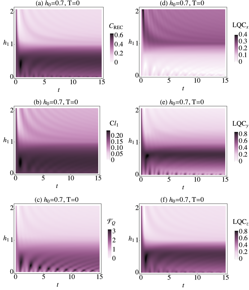
Figure 1: (Color online) Density plots of: (a) the relative entropy of quantum coherence (${\rm C_{REC}}$), (b) the $l_{1}$-norm of quantum coherence (Cl₁), (c) the quantum Fisher information (QFI), and (d-f) local quantum coherence (${\rm LQC_{\alpha}}$) with $\alpha=x,y,z$, versus $t$ and $h_{1}$, at zero temperature and for $h_{0}=0.7$ ($h_{0}<h_{c}$).

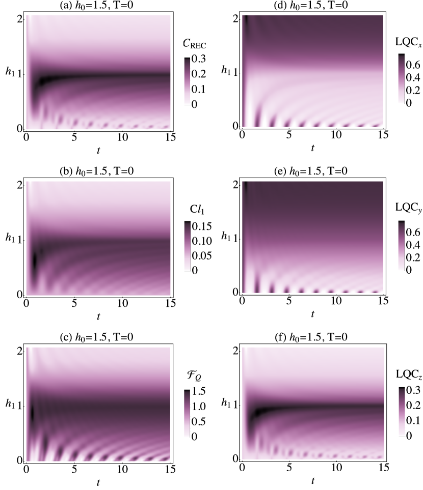
Figure 2: (Color online) Same density plots as Fig. 1 but for the case of $h_{0}=1.5$ ($h_{0}>h_{c}$).

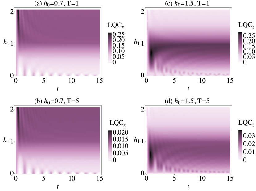
Figure 3: (Color online) The density plots of the local quantum coherence versus $t$, and $h_{1}$, for the different temperatures of $T=1$ and $T=5$. (a and b) show the ${\rm LQC_{x}}$ for $h_{0}=0.7$, and (c and d) represent the ${\rm LQC_{z}}$ for $h_{0}=1.5$.

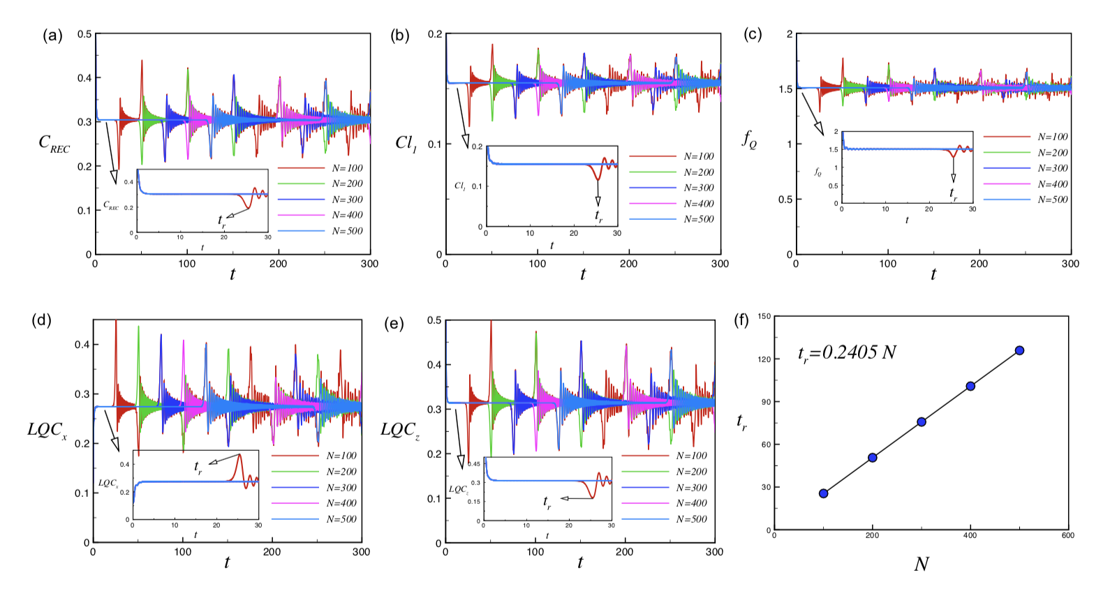
Figure 4: (Color online) The evolution of (a) the relative entropy of quantum coherence, (b) the $l_{1}$-norm of quantum coherence (c) the quantum Fisher information $\mathcal{F}_{Q}$, and (d and e) local quantum coherence, for a quench to the critical point $h_{1}=h_{c}$, for $h_{0}=0.7$ at zero temperature and for the different system sizes. (f) shows the linear behaviour of the first suppression-time (revival-time), $t_{r}(N)$, versus the system size.

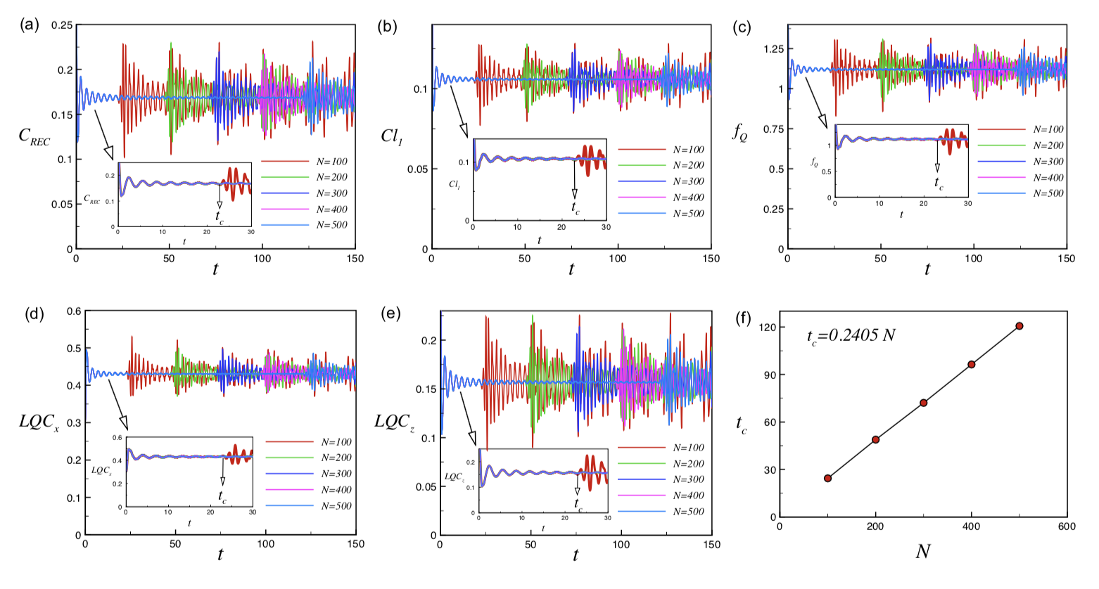
Figure 5: (Color online) (a-e) The same plots as Fig. 4(a-e) but for the case that the system is at the critical point $h_{0}=h_{c}$, and quenched to $h_{1}=1.5$. All plots shows again an oscillating behaviour after the time $t_{c}$, which scales linearly versus the system size shown in (f).

IV Numerical Results and Discussions

We now come to present our numerical results. Although our formalism was for a general case, for simplicity we restrict our discussion to the time dependent transverse magnetic field i.e., $J_{1}=J_{0}=1$. Furthermore, in the main text we only consider time dependent transverse filed Ising model (TFIM) by setting $\gamma=1$, and for more general cases, $\gamma\neq 1$, one can look at the Appendix B. It is well-known that the ground state of the TFIM is characterised by a quantum phase transition that takes place at the critical point $h_{c}=J_{0}$ Pfeuty (1970); McCoy (1968). This phase transition is a result of the quantum fluctuations at zero temperature, which destroy the quantum correlations in the ground state. It is determined via the order parameter, $\langle M^{x}\rangle$, which differs from a finite value for $h<h_{c}$ to zero for $h\geq h_{c}$. Moreover, the ground state is ferromagnetic aligned in $x$-direction for zero magnetic field and it has a paramagnetic alignment along the field for the limit of large magnetic field. Both cases are minimally entangled since the ground state is a product of individual spin states pointing in the $z$- ($x$-) direction as $h\rightarrow\infty$ ($h\rightarrow 0$) Pfeuty (1970); McCoy (1968). Furthermore, by raising the temperature the entanglement shows a sudden decay near the critical point, although at zero temperature and in a vicinity of critical point remains constant Osborne and Nielsen (2002).

IV.1 Quench away from the critical point

In Fig. 1, we plot the intensity of the relative entropy of coherence (a), the $l_{1}$-norm of coherence (b), the quantum Fisher information (c), and local quantum coherence components (d-f), versus $t$ and $h_{1}$. The plots are for $h_{0}=0.7$, and at zero temperature. As one can see, for zero $h_{1}$, where the spins are completely aligned in the $x$-direction, all quantities (expect C$l_{1}$) show an oscillatory behaviour in time. By introducing an external magnetic field, $h_{1}$, the magnitude of quantities increases as field increases until they reach their maximum value close to $h_{1}^{M}=h_{1}\approx 0.5$. In different circumstances, the maximum values of LQC_x occurs at the equilibrium critical point $h_{1}^{M}=h_{1}=h_{c}$. As $h_{1}$ exceeds $h_{1}^{M}$, magnitude of all quantities decrease gradually by magnetic field. Thus, when the system initially is prepared in ferromagnetic phase, $M^{x}(t,T=0)\neq 0$, the maximum of two-spin $S^{x}$ local coherence occurs at the equilibrium critical point and LQC_x is the only quantity can capture truly the critical point. It should be mention that, when the system is prepared in its critical point, $h_{0}=h_{c}$, the maximum value that quantities can reach is much greater than the previous case and appears at $h_{1}^{M}=h_{1}=h_{c}$.

To further elaborate on the behaviour of the zero temperature dynamics above the transition field, $h_{0}>h_{c}$, Fig. 2 presents the intensity of the relative entropy of coherence (a), the $l_{1}$-norm of coherence (b), the quantum Fisher information (c), and local quantum coherence components (d-f), versus $t$ and $h_{1}$. We assume $h_{0}=1.5$, where the system initially prepared at paramagnetic phase, $M^{z}(t,T=0)\neq 0$. As seen, for $h_{1}=0$, all quantities show an oscillatory behavior in time. Besides, when the external magnetic field is turned on ($h_{1}>0$), the magnitude of all quantities except LQC_x and LQC_y, enhances until they reach their maximum value at the equilibrium critical point $h_{1}^{M}=h_{1}=h_{c}$, then reduces by increasing the magnetic field. From these findings one can conclude that dynamical two-spin local $S^{z}$, quantum coherence (WYSI), can positively pick out the critical point while the REC, QFI, and C$l_{1}$ fail in this task. To summarize: Depends on the initial state which the system is prepared, dynamics of the proper component of local quantum coherence can capture the critical point of the system. In other words, when the system is prepared in the initial state with $M^{\alpha}\neq 0$, the dynamics of LQC_α reaches its maximum value at the critical point.

On top of that, there would be a great interest to study the effect of temperature on the critical behavior of many body systems such as the spin systems Sondhi et al. (1997); Osborne and Nielsen (2002); Arnesen et al. (2001); Gunlycke et al. (2001). To show whether the WYSI is able to pinpoint the critical point at finite temperature, we plot the LQC_x and LQC_z in Fig. 3 for different temperatures, namely $T=1,$  and $T=5$. Although the maximum value of LQC decreases as the temperature increases, the equilibrium phase transition point can still be signalled by the maximum of LQC_x and LQC_z at low temperature. This significant property can be easily applied to determine quantum critical points of the systems which today’s technology makes it virtually impossible to achieve the necessary temperature that quantum fluctuations are dominated.

IV.2 Quench from/to the critical point

The time evolution of REC, C$l_{1}$, QFI, and LQC are plotted for a quench to the critical point $h_{1}=1$, for $h_{0}=0.7$ in Fig. 4, for different system sizes. As is clear, in a very short time all quantities change rapidly from the equilibrium state to their average (constant) value that they oscillate around. More than that, all quantities show suppressions and revivals as deviations from the average value. In order to study the effect of the system size on revival/suppression time, $t_{r}$, we also plot $t_{r}(N)$ versus the system size in Fig. 4(f). As seen, the $t_{r}$ increases linearly by the system size, i.e.

$$t_{r}(N)=\tau N,$$ (28)

where the scaling ratio is obtained as $\tau=0.2405$. A more detailed analysis shows that $t_{r}$ and $\tau$ are the same for all quenches and do not depend on the initial preparation phase of system. This is the promised universality of revival/suppression time, which shows that the size of the quench (different values of $h_{0}$) and the initial phase of system are unimportant.

We also demonstrate in Fig. 5 the evolution of REC, C$l_{1}$, QFI, and LQC for $h_{1}=1.5$ and $h_{0}=h_{c}$, where the system prepared initially at the critical point. Applying the external magnetic field causes a rapidly change in all quantities from the equilibrium state to a constant value, before starting oscillations at the time $t_{c}(N)$ [See the insets in Figs. 5(a-e)]. In principle, $t_{c}(N)$ is an instances time under which all curves correspond to a system larger than size $N$, clearly join together. Examining the details in Fig. 5(f), also shows a linear behavior of $t_{c}$ versus $N$,

$$t_{c}(N)=\tau_{c}N,$$ (29)

and interestingly we find a similar scaling value as revival/suppression time, namely $\tau_{c}=\tau=0.2405$. Our calculations show that $t_{c}$ and $\tau_{c}$ are the same for all quenches and do not depend on the phase of system where it quenched to. This is the promised universality of $t_{c}$ which shows that the size of the quench (different values of $h_{1}$) and the phase of system, where the system is quenched to, are ineffectual.

Finally, we study the dynamics of REC, C$l_{1}$, WYSI and QFI for anisotropic case $\gamma\neq 0$. Our numerical analysis show that our previous findings are correct for anisotropic case (see Appendix B). It is worthwhile to mention that, for the case $\gamma<0$, when the system is initialized at the phase with $M^{y}(t,T=0)\neq 0$, the critical point of the system is signalled by the maximum of LQC_y (see Appendix B). Moreover, the numerical simulation shows that $t_{r}$, $t_{c}$ and their scaling ratios, $\tau$ and $\tau_{c}$ are independent of the anisotropy parameter.

V Summary

We have reported the dynamical behaviour of quantum coherence in the one dimensional time-dependent transverse magnetic field XY-model. For this purpose, we investigate the dynamics of relative entropy of coherence, $l_{1}$-norm of coherence, Wigner-Yanase-skew information, and quantum Fisher information. We show that, the phase-transition point can be signalled by the maximum of Wigner-Yanase-skew information local components even at low temperature. While relative entropy of coherence, $l_{1}$-norm of coherence and quantum Fisher information lack such an indicator of criticality in the model. In addition, we find that all of these quantities show suppressions and revivals by quenching the system to the critical point. Further, the first suppression (revival) time scales linearly with system size, and free from the quench size and the initial phase of system, therefore our work highlights the universality in out-of-equilibrium quantum many-body systems.

The success of Wigner-Yanase-skew information dynamics to reveal the equilibrium phase transition may originate from its dependence on the square root of the elements of the density matrix. Therefore, It is a meaningful proposal to study the dynamics of similar quantifiers with a functionality of the square root of the elements of the density matrix. Moreover, it will be interesting to extend the current investigation to more general time-dependent cases of the external magnetic field, such as exponential or periodic functions, and also it is worthwhile to extend the calculation to disorder case.

Appendix A Two point correlation functions of time dependent XY model

Using Eqs. (6, and 7) the expectation value of the magnetization along the $z$-direction, specifically, is given by Barouch et al. (1970); Barouch and McCoy (1971); Sadiek et al. (2010); Huang and Kais (2006); Mishra et al. (2016),

$$\langle M^{z}\rangle=\frac{1}{4N}\sum_{p=1}^{N/2}\frac{\tanh[\beta\Gamma(h_{0},J_{0})]}{\Gamma^{2}(h_{1},J_{1})\Gamma(h_{0},J_{0})}\Bigg{[}2J_{1}(J_{0}h_{1}-J_{1}h_{0})\delta_{p}^{2}\sin^{2}[2t\Gamma(h_{1},J_{1})]+4\Gamma^{2}(h_{1},J_{1})(J_{0}\cos\phi_{p}+h_{0})\Bigg{]},$$ (30)

where $\phi_{p}=2\pi p/N$ , $\delta_{p}=2\gamma\sin\phi_{p}$ and $\beta=1/K_{B}T$. Here $K_{B}$ is Boltzmann constant and $T$ is the temperature. One can simply use the Wick Theorem Wick (1950) to obtain the nearest-neighbor spin correlation functions as follows

$$\langle S^{x}_{l}S^{x}_{l+1}\rangle=\frac{1}{4}F_{l,l+1};\;\;\;\langle S^{y}_{l}S^{y}_{l+1}\rangle=\frac{1}{4}F_{l+1,l};\;\;\;\langle S^{z}_{l}S^{z}_{l+1}\rangle=\frac{1}{4}\Big{[}F_{l,l}\times F_{l+1,l+1}-Q_{l,l+1}\times G_{l,l+1}-F_{l+1,l}\times F_{l,l+1}\Big{]},$$ (31)

in which by defining $\Gamma[h(t),J(t)]=\Big{[}J(t)\cos\phi_{p}+h(t)]^{2}+\gamma^{2}J^{2}(t)\sin^{2}\phi_{p}\Big{]}^{\frac{1}{2}}$, we can write

$$Q_{l,m} =\frac{1}{N}\sum_{p=1}^{N/2}\Bigg{[}2\cos[(m-l)\phi_{p}]+\frac{i(J_{1}h_{0}-J_{0}h_{1})\delta_{p}\sin[(m-l)\phi_{p}]\sin[4t\Gamma(h_{1},J_{1})]\tanh[\beta\Gamma(h_{0},J_{0})]}{\Gamma(h_{1},J_{1})\Gamma(h_{0},J_{0})}\Bigg{]},\quad$$ (32)

$$G_{l,m} =\frac{1}{N}\sum_{p=1}^{N/2}\Bigg{[}-2\cos[(m-l)\phi_{p}]+\frac{i(J_{1}h_{0}-J_{0}h_{1})\delta_{p}\sin[(m-l)\phi_{p}]\sin[4t\Gamma(h_{1},J_{1})]\tanh[\beta\Gamma(h_{0},J_{0})]}{\Gamma(h_{1},J_{1})\Gamma(h_{0},J_{0})}\Bigg{]},\quad$$

$$F_{l,m}= \frac{1}{N}\sum_{p=1}^{N/2}\frac{\tanh[\beta\Gamma(h_{0},J_{0})]}{\Gamma^{2}(h_{1},J_{1})\Gamma(h_{0},J_{0})}\Bigg{[}\cos[(m-l)\phi_{p}]\times\Big{[}J_{1}[J_{0}h_{1}-J_{1}h_{0}]\delta^{2}_{p}\sin^{2}[2t\Gamma(h_{1},J_{1})]+2\Gamma^{2}(h_{1},J_{1})(J_{0}\cos\phi_{p}+h_{0})\Big{]}$$ (33)

$$+\delta_{p}\sin[(m-l)\phi_{p}]\Big{[}J_{0}\Gamma^{2}(h_{1},J_{1})+2(J_{1}h_{0}-J_{0}h_{1})(J_{1}\cos\phi_{p}+h_{1})\sin^{2}[2t\Gamma(h_{1},J_{1})]\Big{]}\Bigg{]}.$$

Appendix B WYSI for anisotropic case $\gamma\neq 0$

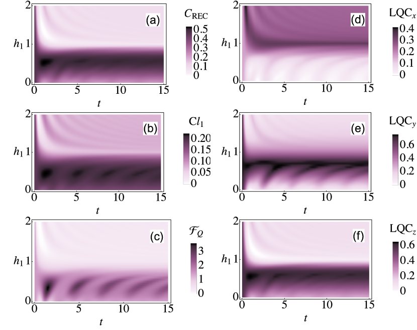
Figure 6: (Color online) Same density plots as Fig. 1 but for the case of $\gamma=0.5$, at zero temperature and for $h_{0}=0.7$ ($h_{0}<h_{c}$).

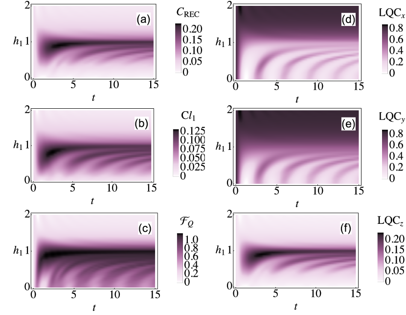
Figure 7: (Color online) Same density plots as Fig. 1 but for the case of $\gamma=0.5$ at zero temperature and $h_{0}=1.5$ ($h_{0}>h_{c}$).

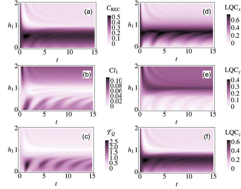
Figure 8: (Color online) Same density plots as Fig. 1 but for the case of $\gamma=-0.5$ at zero temperature and $h_{0}=0.7$ ($h_{0}<h_{c}$) with magnetisation along the $y$-direction.

In this appendix, we study the dynamics of the quantities for anisotropic case $\gamma\neq 0$ (Eq. 1). For this purpose in the Fig. 6, we first look at the anisotropic case $\gamma=0.5$. We show the density plot of dynamical behaviour of the relative entropy of coherence (a), the $l_{1}$-norm of coherence (b), the quantum Fisher information (c), and local quantum coherence components (d-f), versus time and $h_{1}$, for $J_{0}=J_{1}=1$, and $h_{0}=0.7$. As we expect, when the initial state prepared in ferromagnetic case $M^{x}\neq 0$, the LQC_x shows maximum at the critical point of the system $h_{c}=1$. Moreover, we show that when the system initialized at paramagnetic phase $M^{z}\neq 0$, i.e., $h_{0}>1$, the LQC_z fulfils the expectation and reaches its maximum at the critical point. This is clearly represented in the results of Fig. 7. Finally, for the case that, the system initially prepared at ferromagnetic phase $\gamma<0$, in which $M^{y}\neq 0$, the maximum of LQC_y happens at the critical point of the system (see Fig. 8). Briefly, one can conclude that when the system is prepared in the initial state with $M^{\alpha}\neq 0$, the dynamics of LQC_α reaches its maximum value at the critical point.

References

- Horodecki et al. (2009) R. Horodecki, P. Horodecki, M. Horodecki, and K. Horodecki, Rev. Mod. Phys. 81, 865 (2009).
- Modi et al. (2012) K. Modi, A. Brodutch, H. Cable, T. Paterek, and V. Vedral, Rev. Mod. Phys. 84, 1655 (2012).
- Ficek and Swain (2005) Z. Ficek and S. Swain, Quantum Interference and Coherence (Springer-Verlag New York, 2005).
- Chuang and Nielsen (2000) I. Chuang and M. Nielsen, Quantum Computation and Quantum Information (Cambridge University Press, Cambridge, 2000).
- Baumgratz et al. (2014) T. Baumgratz, M. Cramer, and M. B. Plenio, Phys. Rev. Lett. 113, 140401 (2014).
- Xi et al. (2015) Z. Xi, Y. Li, and H. Fan, Scientific Reports 5, 10922 (2015).
- Hu and Fan (2016) M.-L. Hu and H. Fan, Scientific Reports 6, 29260 (2016).
- Qin et al. (2018) M. Qin, Z. Ren, and X. Zhang, Phys. Rev. A 98, 012303 (2018).
- (9) L. Balazadeh, G. Najarbashi, and A. Tavana, 10.1007/s11128-020-02677-7.
- Rana et al. (2016) S. Rana, P. Parashar, and M. Lewenstein, Phys. Rev. A 93, 012110 (2016).
- Girolami (2014) D. Girolami, Phys. Rev. Lett. 113, 170401 (2014).
- Huang et al. (2009) J.-F. Huang, Y. Li, J.-Q. Liao, L.-M. Kuang, and C. P. Sun, Phys. Rev. A 80, 063829 (2009).
- Huang (2017) Z. Huang, Quantum Information Processing 16, 207 (2017).
- Lei and Tong (2016) S. Lei and P. Tong, Quantum Information Processing 15, 1811 (2016).
- Mzaouali and Baz (2019) Z. Mzaouali and M. E. Baz, Physica A: Statistical Mechanics and its Applications 518, 119 (2019).
- Wigner and Yanase (1963) E. P. Wigner and M. M. Yanase, Proceedings of the National Academy of Sciences 49, 910 (1963).
- Luo (2003) S. Luo, Phys. Rev. Lett. 91, 180403 (2003).
- Fisher (1925) R. A. Fisher, Mathematical Proceedings of the Cambridge Philosophical Society 22, 700 (1925).
- Helstrom (1976) C. W. Helstrom, Quantum detection and estimation theory, Math. Sci. Eng. (Academic Press, New York, NY, 1976).
- Frieden and Soffer (1995) B. R. Frieden and B. H. Soffer, Phys. Rev. E 52, 2274 (1995).
- Frieden (2000) B. R. Frieden, American Journal of Physics 68, 1064 (2000), https://doi.org/10.1119/1.1308267 .
- Zhang et al. (2018) Y.-R. Zhang, Y. Zeng, H. Fan, J. Q. You, and F. Nori, Phys. Rev. Lett. 120, 250501 (2018).
- Taddei et al. (2013) M. M. Taddei, B. M. Escher, L. Davidovich, and R. L. de Matos Filho, Phys. Rev. Lett. 110, 050402 (2013).
- Gibilisco et al. (2007) P. Gibilisco, D. Imparato, and T. Isola, Journal of Mathematical Physics 48, 072109 (2007), https://doi.org/10.1063/1.2748210 .
- Karpat et al. (2014) G. Karpat, B. Çakmak, and F. F. Fanchini, Phys. Rev. B 90, 104431 (2014).
- Invernizzi et al. (2008) C. Invernizzi, M. Korbman, L. Campos Venuti, and M. G. A. Paris, Phys. Rev. A 78, 042106 (2008).
- Sun et al. (2010) Z. Sun, J. Ma, X.-M. Lu, and X. Wang, Phys. Rev. A 82, 022306 (2010).
- Holevo (1982) A. S. Holevo, Probabilistic and Statistical Aspects of Quantum Theory, Math. Sci. Eng. (Edizioni della Normale, New York, NY, 1982).
- Braunstein and Caves (1994a) S. L. Braunstein and C. M. Caves, Phys. Rev. Lett. 72, 3439 (1994a).
- Braunstein et al. (1996) S. L. Braunstein, C. M. Caves, and G. Milburn, Annals of Physics 247, 135 (1996).
- Wang et al. (2016) J. Wang, Z. Tian, J. Jing, and H. Fan, Phys. Rev. A 93, 062105 (2016).
- Liu et al. (2016) X. Liu, Z. Tian, J. Wang, and J. Jing, Annals of Physics 366, 102 (2016).
- Hu (2016) X. Hu, Phys. Rev. A 94, 012326 (2016).
- Yao et al. (2016) Y. Yao, G. H. Dong, X. Xiao, and C. P. Sun, Scientific Reports 6, 32010 (2016).
- Hillery (2016) M. Hillery, Phys. Rev. A 93, 012111 (2016).
- Ma et al. (2016) J. Ma, B. Yadin, D. Girolami, V. Vedral, and M. Gu, Phys. Rev. Lett. 116, 160407 (2016).
- Matera et al. (2016) J. M. Matera, D. Egloff, N. Killoran, and M. B. Plenio, Quantum Science and Technology 1, 01LT01 (2016).
- Braunstein and Caves (1994b) S. L. Braunstein and C. M. Caves, Phys. Rev. Lett. 72, 3439 (1994b).
- Giovannetti et al. (2006) V. Giovannetti, S. Lloyd, and L. Maccone, Phys. Rev. Lett. 96, 010401 (2006).
- Polkovnikov et al. (2011) A. Polkovnikov, K. Sengupta, A. Silva, and M. Vengalattore, Rev. Mod. Phys. 83, 863 (2011).
- Pappalardi et al. (2017) S. Pappalardi, A. Russomanno, A. Silva, and R. Fazio, Journal of Statistical Mechanics: Theory and Experiment 2017, 053104 (2017).
- Häppölä et al. (2012) J. Häppölä, G. B. Halász, and A. Hamma, Phys. Rev. A 85, 032114 (2012).
- Jafari and Johannesson (2017a) R. Jafari and H. Johannesson, Phys. Rev. Lett. 118, 015701 (2017a).
- Jafari and Johannesson (2017b) R. Jafari and H. Johannesson, Phys. Rev. B 96, 224302 (2017b).
- Jafari et al. (2019) R. Jafari, H. Johannesson, A. Langari, and M. A. Martin-Delgado, Phys. Rev. B 99, 054302 (2019).
- Mishra et al. (2018) U. Mishra, H. Cheraghi, S. Mahdavifar, R. Jafari, and A. Akbari, Phys. Rev. A 98, 052338 (2018).
- Jafari (2019) R. Jafari, Scientific reports 9, 1 (2019).
- Jafari and Akbari (2015) R. Jafari and A. Akbari, EPL (Europhysics Letters) 111, 10007 (2015).
- Jafari (2010) R. Jafari, Phys. Rev. A 82, 052317 (2010).
- Jafari (2016) R. Jafari, Journal of Physics A: Mathematical and Theoretical 49, 185004 (2016).
- Barouch et al. (1970) E. Barouch, B. M. McCoy, and M. Dresden, Phys. Rev. A 2, 1075 (1970).
- Barouch and McCoy (1971) E. Barouch and B. M. McCoy, Phys. Rev. A 3, 786 (1971).
- Sadiek et al. (2010) G. Sadiek, B. Alkurtass, and O. Aldossary, Phys. Rev. A 82, 052337 (2010).
- Huang and Kais (2006) Z. Huang and S. Kais, Phys. Rev. A 73, 022339 (2006).
- Mishra et al. (2016) U. Mishra, D. Rakshit, and R. Prabhu, Phys. Rev. A 93, 042322 (2016).
- Streltsov et al. (2017) A. Streltsov, G. Adesso, and M. B. Plenio, Rev. Mod. Phys. 89, 041003 (2017).
- Çakmak et al. (2012) B. Çakmak, G. Karpat, and Z. Gedik, Physics Letters A 376, 2982 (2012).
- Li and Luo (2013) N. Li and S. Luo, Phys. Rev. A 88, 014301 (2013).
- Chin et al. (2012) A. W. Chin, S. F. Huelga, and M. B. Plenio, Phys. Rev. Lett. 109, 233601 (2012).
- Liu et al. (2013) J. Liu, X. Jing, and X. Wang, Phys. Rev. A 88, 042316 (2013).
- Zhang et al. (2013) Y. M. Zhang, X. W. Li, W. Yang, and G. R. Jin, Phys. Rev. A 88, 043832 (2013).
- Pfeuty (1970) P. Pfeuty, Annals of Physics 57, 79 (1970).
- McCoy (1968) B. M. McCoy, Phys. Rev. 173, 531 (1968).
- Osborne and Nielsen (2002) T. J. Osborne and M. A. Nielsen, Phys. Rev. A 66, 032110 (2002).
- Sondhi et al. (1997) S. L. Sondhi, S. M. Girvin, J. P. Carini, and D. Shahar, Rev. Mod. Phys. 69, 315 (1997).
- Arnesen et al. (2001) M. C. Arnesen, S. Bose, and V. Vedral, Phys. Rev. Lett. 87, 017901 (2001).
- Gunlycke et al. (2001) D. Gunlycke, V. M. Kendon, V. Vedral, and S. Bose, Phys. Rev. A 64, 042302 (2001).
- Wick (1950) G. C. Wick, Phys. Rev. 80, 268 (1950).