Variable-lag Granger Causality and Transfer Entropy for Time Series Analysis

Abstract.

Granger causality is a fundamental technique for causal inference in time series data, commonly used in the social and biological sciences. Typical operationalizations of Granger causality make a strong assumption that every time point of the effect time series is influenced by a combination of other time series with a fixed time delay. The assumption of fixed time delay also exists in Transfer Entropy, which is considered to be a non-linear version of Granger causality. However, the assumption of the fixed time delay does not hold in many applications, such as collective behavior, financial markets, and many natural phenomena. To address this issue, we develop Variable-lag Granger causality and Variable-lag Transfer Entropy, generalizations of both Granger causality and Transfer Entropy that relax the assumption of the fixed time delay and allow causes to influence effects with arbitrary time delays. In addition, we propose methods for inferring both variable-lag Granger causality and Transfer Entropy relations. In our approaches, we utilize an optimal warping path of Dynamic Time Warping (DTW) to infer variable-lag causal relations. We demonstrate our approaches on an application for studying coordinated collective behavior and other real-world casual-inference datasets and show that our proposed approaches perform better than several existing methods in both simulated and real-world datasets. Our approaches can be applied in any domain of time series analysis. The software of this work is available in the R-CRAN package: VLTimeCausality.

1. Introduction

Inferring causal relationships from data is a fundamental problem in statistics, economics, and science in general. The gold standard for assessing causal effects is running randomized controlled trials which randomly assign a treatment (e.g., a drug or a specific user interface) to a subset of a population of interest, and randomly select another subset as a control group which is not given the treatment, thus attributing the outcome difference between the two groups to the treatment. However, in many cases, running such trials may be unethical, expensive, or simply impossible (Varian, 2016). To address this issue, several methods have been developed to estimate causal effects from observational data (Pearl, 2000; Spirtes et al., 1993).

In the context of time series data, a well-known method that defines a causal relation in terms of predictability is Granger causality (Granger, 1969). $X$ Granger-causes $Y$ if past information on $X$ predicts the behavior of $Y$ better than $Y$’s past information alone (Arnold et al., 2007). In this work, when we refer to causality, we mean specifically the predictive causality defined by Granger causality. The key assumptions of Granger causality are that 1) the process of effect generation can be explained by a set of structural equations, and 2) the current realization of the effect at any time point is influenced by a set of causes in the past. Similar to other causal inference methods, Granger causality assumes unconfoundedness and that all relevant variables are included in the analysis (Granger, 1969; Peters et al., 2017).

There are several studies that have been developed based on Granger causality  (Liu et al., 2012; Atukeren et al., 2010; Peters et al., 2013).

Granger causality is typically studied in the context of linear structural equations. Transfer Entropy has been developed as a non-linear extension of Granger causality (Schreiber, 2000; Lee et al., 2012; Barnett et al., 2009).

The typical operational definitions (Atukeren et al., 2010) and inference methods for inferring Granger causality, including the common software implementation packages (MLS, [n. d.]; RSo, [n. d.]), assume that the effect is influenced by the cause with a fixed and constant time delay.

However, the assumption of an effect is fixed-lag influenced by the cause still exists in both Granger causality and transfer entropy.

This assumption of a fixed and constant time delay between the cause and effect is, in fact, too strong for many applications of understanding natural world and social phenomena. In such domains, data is often in the form of a set of time series and a common question of interest is which time series are the (causal) initiators of patterns of behaviors captured by another set of time series. For example, who are the individuals who influence a group’s direction in collective movement? What are the sectors that influence the stock market dynamics right now? Which part of the brain is critical in activating a response to a given action? In all of these cases, effects follow the causal time series with delays that can vary over time (Amornbunchornvej et al., 2018). The fact that one time series can be caused by multiple initiators and these initiators can be inferred from time series data (Amornbunchornvej et al., 2018; Arnold et al., 2007).

To address the remaining gap, we introduce the concepts Variable-lag Granger causality and Variable-lag Transfer Entropy and methods to infer them in time series data. We prove that our definitions and the proposed inference methods can address the arbitrary-time-lag influence between cause and effect, while the traditional operationalizations of Granger causality, transfer entropy, and their corresponding inference methods cannot. We show that the traditional definitions are indeed special cases of the new relations we define. We demonstrate the applicability of the newly defined causal inference frameworks by inferring initiators of collective coordinated movement, a problem proposed in (Amornbunchornvej et al., 2018), as well as inferring casual relations in other real-world datasets.

We use Dynamic Time Warping (DTW) (Sakoe and Chiba, 1978) to align the cause $X$ to the effect time series $Y$ while leveraging the power of Granger causality and transfer entropy. In the literature, there are many clustering-based Granger causality methods that use DTW to cluster time series and perform Granger causality only for time series within the same clusters (Yuan et al., 2016; Peng et al., 2007). Previous work on inferring causal relations using both Granger causality and DTW has the assumption that the smaller warping distance between two time series, the stronger the causal relation is (Sliva et al., 2015). If the minimum distance of elements within the DTW optimal warping path is below a given distance threshold, then the method considers that there is a causal relation between the two time series. However, their work assumes that Granger causality and DTW run independently. In contrast, our method formalizes the integration of Granger causality and DTW by generalizing the definition of Granger causality itself and using DTW as an instantiation of the optimal alignment requirement of the time series.

In addition to the standard uses of Granger causality and transfer entropy, our methods are capable of:

• Inferring arbitrary-lag causal relations: our methods can infer a causal relation of Granger or transfer entropy where a cause influences an effect with arbitrary delays that can change dynamically;

• Quantifying variable-lag emulation: our methods can report the similarity of time series patterns between the cause and the delayed effect, for arbitrary delays;

We also prove that when multiple time series cause the behavioral convergence of a set of time series then we can treat the set of these initiating causes in the aggregate and there is a causal relation between this aggregate cause (of the set of initiating time series) and the aggregate of the rest of the time series. We provide many experiments and examples using both simulated and real-world datasets to measure the performance of our approach in various causality settings and discuss the resulting domain insights. Our framework is highly general and can be used to analyze time series from any domain.

2. Related work

Granger causality has inspired a lot of research since its introduction in 1969 (Granger, 1969). Recent works on Granger causality has focused on various generalizations for it, including ones based on information theory, such as transfer entropy (Schreiber, 2000; Shibuya et al., 2009) and directed information graphs (Quinn et al., 2015). Recent inference methods are able to deal with missing data (Iseki et al., 2019) and enable feature selection (Sun et al., 2015). Granger causality has even been explored as a method to offer explainability of machine learning models (Schwab et al., 2019). However, none of them study tests for Variable-lag Granger causality, as we formalize and propose in this work.

Many causal inference methods assume that the data is i.i.d. and rely on knowing a mechanism that generates that data, e.g., expressed through causal graphs or structural equations (Pearl, 2000). In time series data, there are two ways in which time series can be i.i.d.: 1) the points of one time series are independent of other points in the same time series, 2) one time series is independent of another time series. Obviously, in most time series, the values of the consecutive time steps violate the i.i.d. assumption (the first way). In causal inference, the field focuses on the independent between two time series in the second way.

Another set of causal inference methods relax this strong i.i.d assumption, and instead assume independence between the cause and the mechanism generating the effect  (Janzing and Scholkopf, 2010; Schölkopf et al., 2012; Shajarisales et al., 2015). Specifically, knowing a distribution of random variable of cause $X$ never reveals information about the structural function $f(X)$ and vice versa. This idea has been used in the context of times series data (Shajarisales et al., 2015) by relying on the concept of Spectral Independence Criterion (SIC). If a cause $X$ is a stationary process that generates the effect $Y$ via linear time invariance filter $h$ (mechanism), then $X$ and $h$ should not contain any information about each other but dependency between them and $Y$ exists in spectral sense.

There is a framework of causal inference in (Malinsky and Spirtes, 2018) based on conditional independence tests on time series generated from some discrete-time stochastic processes that allows unknown latent variables. However, the approach in (Malinsky and Spirtes, 2018) still assumes that data points at any time step have been generated from some structural vector autoregression (SVAR). The recent work in (Griveau-Billion and Calderhead, 2019) models causal relation between time series as a form of polynomial function and uses a stochastic block model to find a causal graph. Both works, however, still have the assumption of fixed-lag influence from causes to effects.

Besides, no method studies a causal structure that is unstable overtime (Eichler, 2013).

Moreover, Transfer Entropy, which is considered to be a non-linear extension of Granger causality (Schreiber, 2000; Lee et al., 2012; Barnett et al., 2009), still has the fixed-lag assumption.

In our work, we also relax the stationary assumption of time series.

3. Extension from previous work

This paper is an extension of our conference proceeding (Amornbunchornvej et al., 2019). In our previous work (Amornbunchornvej et al., 2019), we formalized VL-Granger causality and proposed a framework to infer a causal relation using BIC and F-test as main criteria to infer whether $X$ causes $Y$.

In this work, we formalize Variable-Lag Transfer Entropy, which is a non-linear extension of Granger-causality. We investigate the challenge of generalizing Transfer Entropy by relaxing its fixed-lag assumption. Then, we propose a framework to infer VL-Transfer Entropy causal relations.

Moreover, we extend our work on VL-Granger Causality and propose to use a Bayesian Information Criterion difference ratio or BIC difference ratio, which is a normalized BIC, as a main criterion. There is evidence that BIC performs better than other model-selection criteria in general (Raffalovich et al., 2008; Granger and Jeon, 2004; Atukeren et al., 2010). We also add two new real-world datasets and additional experiments in this current work.

4. Granger causality and fixed lag limitation

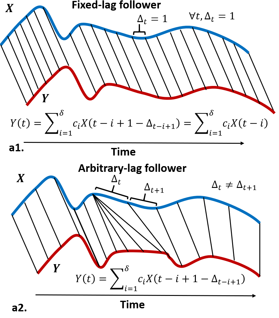
Figure 1. (a1-2.) A leader (blue) influences a follower (red) at a specific time point via black lines. (a1.) The follower is a distorted version of a leader with a fixed lag. (a2.) The follower is a distorted version of a leader with non-fixed lags in that violates an assumption of Granger causality. Granger causality can handle only the former case and typically fails to handle later case. We propose the generalization of Granger causality to handle variable-lag situation (equation in a2.).

Let $X=(X(1),\dots,X(t),\dots)$ be a time series. We will use $X(t)\in\mathbb{R}$ to denote an element of $X$ at time $t$. Given two time series $X$ and $Y$, it is said that $X$ Granger-causes (Granger, 1969) $Y$ if the information of $X$ in the past helps improve the prediction of the behavior of $Y$, over $Y$’s past information alone (Arnold et al., 2007). The typical way to operationalize this general definition of Granger causality  (Atukeren et al., 2010) is to define it as follows:

Definition 4.1 (Granger causal relation).

Let $X$ and $Y$ be time series, and $\delta_{max}\in\mathbb{N}$ be a maximum time lag. We define two residuals of regressions of $X$ and $Y$, $r_{Y},r_{YX}$, below:

(1) $$r_{Y}(t)=Y(t)-\sum_{i=1}^{\delta_{max}}a_{i}Y(t-i),$$

(2) $$r_{YX}(t)=Y(t)-\sum_{i=1}^{\delta_{max}}(a_{i}Y(t-i)+b_{i}X(t-i)),$$

where $a_{i}$ and $b_{i}$ are constants that optimally minimize the residual from the regression. Then $X$ Granger-causes $Y$ if the variance of $r_{YX}$ is less than the variance of $r_{Y}$.

This definition assumes that, for all $t>0$, $Y(t)$ can be predicted by the fixed linear combination of $a_{1}Y(1),\dots,a_{t-\Delta}Y(t-\Delta)$ and $b_{1}X(1),\dots,b_{t-\Delta}X(t-\Delta)$ with some fixed $\Delta>0$ and every $a_{i},b_{i}$ is a fixed constant over time (Atukeren et al., 2010; Arnold et al., 2007). However, in reality, two time series might influence each other with a sequence of arbitrary, non-fixed time lags. For example, Fig. 1(a2.) has $X$ as a cause time series and $Y$ as the effect time series that imitates the values of $X$ with arbitrary lags. Because $Y$ is not affected by $X$ with a fixed lags and the linear combination above can change over time, the standard Granger causality tests cannot appropriately infer Granger-causal relation between $X$ and $Y$ even if $Y$ is just a slightly distorted version of $X$ with some lags. For a concrete example, consider a movement context where time series represent trajectories. Two people follow each other if they move in the same trajectory. Assuming the followers follow leaders with a fixed lag means the followers walk lockstep with the leader, which is not the natural way we walk. Imagine two people embarking on a walk. The first starts walking, the second catches up a little later. They may walk together for a bit, then the second stops to tie the shoe and catches up again. The delay between the first and the second person keeps changing, yet there is no question the first sets the course and is the cause of the second’s choices where to go. Fig. 1 illustrates this example.

5. Variable-lag Granger Causality

Here, we propose the concept of variable-lag Granger causality, VL-Granger causality for short, which generalizes the Granger causal relation of Definition 4.1 in a way that addresses the fixed-lag limitation. We demonstrate the application of the new causality relation for a specific application of inferring initiators and followers of collective behavior.

Definition 5.1 (Alignment of time series).

An alignment between two time series $X$ and $Y$ is a sequence of pairs of indices $(t_{i},t_{j})$, aligning $X(t_{i})$ to $Y(t_{j})$, such that for any two pairs in the alignment $(t_{i},t_{j})$ and $(t^{\prime}_{i},t^{\prime}_{j})$, if $t_{i}<t^{\prime}_{i}$ then $t_{j}<t^{\prime}_{j}$ (non-crossing condition). The alignment defines a sequence of delays $P=(\Delta_{1},\dots,\Delta_{t},\dots)$, where $\Delta_{t}\in\mathbb{Z}$ and $X(t-\Delta_{t})$ aligns to $Y(t)$.

Definition 5.2 (VL-Granger causal relation).

Let $X$ and $Y$ be time series, and $\delta_{max}\in\mathbb{N}$ be a maximum time lag (this is an upper bound on the time lag between any two pairs of time series values to be considered as causal). We define residual $r^{*}_{YX}$ of the regression:

(3) $$r^{*}_{YX}(t)=Y(t)-\sum_{i=1}^{\delta_{max}}(a_{i}Y(t-i)+b_{i}X(t-i)+c_{i}X^{*}(t-i)).$$

Here $X^{*}(t-i)=X(t-i+1-\Delta_{t-i+1})$, where $\Delta_{t}>0$ is a time delay constant in the optimal alignment sequence $P^{*}$ of $X$ and $Y$ that minimizes the residual of the regression. The constants $a_{i},b_{i}$, and $c_{i}$ optimally minimize the residuals $r_{Y}$, $r_{YX}$, and $r^{*}_{YX}$, respectively. The terms $b_{i}$ and $c_{i}$ can be combined but we keep them separate to clearly denote the difference between the original and proposed VL-Granger causality. We say that $X$ VL-Granger-causes $Y$ if the variance of $r^{*}_{YX}$ is less than the variances of both $r_{Y}$ and $r_{YX}$.

In order to make Definition 5.2 fully operational for this more general case (and to find the optimal constants values), we need a similarity function between two sequences which will define the optimal alignment. We propose such a similarity-based approach in Definition 5.5. Before defining this approach, we show that VL-Granger causality is the proper generalization of the traditional operational definition of Granger causality stated in Definition 4.1. Clearly, assuming that all delays are less than $\delta_{max}$, if all the delays are constant, then $r^{*}_{YX}(t)=r_{YX}(t)$.

Proposition 5.3.

Let $X$ and $Y$ be time series and $P$ be their alignment sequence. If $\forall t,\Delta_{t}=\Delta$, then $r^{*}_{YX}(t)=r_{YX}(t)$.

We must also show that the variance of $r^{*}_{YX}(t)$ is no greater than the variance of $r_{YX}(t)$.

Proposition 5.4.

Let $X$ and $Y$ be time series, $P=(\Delta_{1},\dots,\Delta_{t},\dots)$ be their alignment sequence such that $Y(t)=X(t-\Delta_{t})$. If $\exists\Delta_{t},\Delta_{t^{\prime}}\in P$, such that $\Delta_{t}\neq\Delta_{t^{\prime}}$ and $\forall t,X(t)\neq X(t-1)$, then $VAR(r^{*}_{YX})<VAR(r_{YX})$.

Proof.

Because $Y(t)=X(t-\Delta_{t})$, by setting $a_{i}=0,b_{i}=0,c_{i}=1$ for all $i$, we have $r^{*}_{YX}=0$. In contrast, suppose $\Delta_{t+1}=\Delta_{t}+1$ and $X(t-\Delta_{t}-1)\neq X(t-\Delta_{t})\neq X(t-\Delta_{t}+1)$, so $Y(t)=Y(t+1)=X(t-\Delta_{t})$. Because $a_{i},b_{i}$ must be constant for all time step $t$ to compute $r_{YX}(t)$, at time $t$, the regression must choose to match either 1) $Y(t)-X(t-\Delta_{t})=0$ and $Y(t+1)-X(t+1-\Delta_{t})\neq 0$ or 2) $Y(t)-X(t-\Delta_{t+1})\neq 0$ and $Y(t+1)-X(t+1-\Delta_{t+1})=0$. Both 1) and 2) options make $r_{YX}(t)+r_{YX}(t+1)>0$. Hence, $VAR(r^{*}_{YX})<VAR(r_{YX})$. ∎

According to Propositions 5.3 and 5.4, VL-Granger causality is the generalization of the Def. 4.1 and always has lower or equal variance.

Of a particular interest is the case when there is an explicit similarity relation defined over the domain of the input time series. The underlying alignment of VL-Granger causality then should incorporate that similarity measure and the methods for inferring the optimal alignment for the given similarity measure.

Definition 5.5 (Variable-lag emulation).

Let $\mathcal{U}$ be a set of time series, $X,Y\in\mathcal{U}$, and $\mathrm{sim}:\mathcal{U}\times\mathcal{U}\to[0,1]$ be a similarity measure between two time series.

For a threshold $\sigma\in(0,1]$, if there exists a sequence of numbers $P=(\Delta_{1},\dots,\Delta_{t},\dots)$ s.t. $\mathrm{sim}(\tilde{X},Y)\geq\sigma$ when $\tilde{X}(t)=X(t-\Delta_{t})$, then we use the following notation:

• if $\forall\Delta_{t}\in P,\>\Delta_{t}\geq 0$ , then $Y$ emulates $X$, denoted by ${X\preceq Y}$,

• if $\forall\Delta_{t}\in P,\>\Delta_{t}\leq 0$ , then $X$ emulates $Y$, denoted by ${Y\preceq X}$,

• if ${X\preceq Y}$ and ${Y\preceq X}$, then ${Y\equiv X}$.

We denote ${X\prec Y}$ if ${X\preceq Y}$ and $\exists\Delta_{t}\in P,\Delta_{t}>0$.

Note, here the sim similarity function does not have to be a distance function that obeys, among others, a triangle inequality. It can be any function that quantitatively compares the two time series. For example, it may be that when one time series increases the other decreases. We provide a more concrete and realistic example in the application setting below.

Adding this similarity measure to Definition 5.2 allows us to instantiate the notion of the optimal alignment $P^{*}$ as the one that maximizes the similarity between $X$ and $Y$:

(4) $$P^{*}=\mathop{\mathrm{argmax}}\limits_{P}\mathrm{sim}(\tilde{X},Y),$$

where $\tilde{X}(t)=X(t-\Delta_{t})$ for any given $P$ and $\Delta_{t}\in P$. With that addition, if $X\prec Y$, then $X$ VL-Granger-causes $Y$. This allows us to operationalize VL-Granger causality by checking for variable-lag emulation, as we describe in the next section.

5.1. Example application: Initiators and followers

In this section, we demonstrate an application of the VL-Granger causal relation to finding initiators of collective behavior. The Variable-lag emulation concept corresponds to a relation of following in the leadership literature (Amornbunchornvej et al., 2018). That is, $X\prec Y$ if $Y$ is a follower of $X$. We are interested in the phenomenon of group convergence to a consensus behavior and answering the question of which subset of individuals, if any, initiated that collective consensus behavior. With that in mind, we now define the concept of an initiator and provide a set of subsidiary definitions that allow us to formally show (in Proposition 5.9) that initiators of collective behavior are indeed the time series that VL-Granger-cause the collective pattern in the set of the time series. In order to do this, we generalize our two-time series definitions to the case of multiple time series by defining the notion of an aggregate time series, which is consistent with previous Granger causality generalizations to multiple time series (Siggiridou and Kugiumtzis, 2016; Eichler, 2013; Chen et al., 2004).

Definition 5.6 (Initiators).

Let $\mathcal{U}=\{U_{1},\dots,U_{n}\}$ be a set of time series. We say that $\mathcal{X}\subseteq\mathcal{U}$ is a set of initiators if $\forall U\in\mathcal{U\setminus\mathcal{X}}$, $\>\exists X\in\mathcal{X}$, $\>s.t.X\prec U$, and, conversely, $\forall X\in\mathcal{X}\>\exists U\in\mathcal{U\setminus\mathcal{X}},\>s.t.X\prec U$. That is, every time series follows some initiator and every initiator has at least one follower.

Given a set of time series $\mathcal{U}=\{U_{1},\dots,U_{n}\}$ , and a set of time series $\mathcal{X}\subseteq\mathcal{U}$, we can define an aggregate time series as a time series of means at each step:

(5) $$agg(\mathcal{X})=\left({\frac{1}{|\mathcal{X}|}\sum_{U\in\mathcal{X}}U(0),\dots,\frac{1}{|\mathcal{X}|}\sum_{U\in\mathcal{X}}U(t),\dots}\right)$$

In order to identify the state of reaching a collective consensus of a time series, while allowing for some noise, we adopt the concept of $\epsilon$-convergence from (Chazelle, 2011).

Definition 5.7 ($\epsilon$-convergence).

Let $Q$ and $U$ be time series, $dist:\mathbb{R}^{2}\times[0,1]$ be a distance function, and $0<\epsilon\leq 1/2$. If for all time $t\in[t_{0},t_{1}],\>dist(Q(t),U(t))\leq\epsilon$, then $Q$ and $U$ $\epsilon$-converge toward each other in the interval $[t_{0},t_{1}]$. If $t_{1}=\infty$ then we say that $Q$ and $U$ $\epsilon$-converge at time $t_{0}$.

Definition 5.8 ($\epsilon$-convergence coordination set).

Given a set of time series $\mathcal{U}=\{U_{1},\dots,U_{n}\}$, if all time series in $\mathcal{U}$ $\epsilon$-converge toward $agg(\mathcal{U})$, then we say that the set $\mathcal{U}$ is an $\epsilon$-convergence coordination set.

We are finally ready to state the main connection between initiation of collective behavior and VL-Granger causality.

Proposition 5.9.

Let $dist:\mathbb{R}^{2}\times[0,1]$ be a distance function, $\mathcal{U}$ be a set of time series, and $\mathcal{X}\subseteq\mathcal{U}$ be a set of initiators, which is an $\epsilon$-convergence coordination set converging towards $agg(\mathcal{X})$ in the interval $[t_{0},t_{1}]$. For any $U,U^{\prime}\in\mathcal{U}$ of length $T$, let

$$\mathrm{sim}(U,U^{\prime})=\frac{\sum_{t}1-dist(U(t),U^{\prime}(t))}{T}.$$

If for any $U,U^{\prime}\in\mathcal{U}$ their similarity $\mathrm{sim}(U,U^{\prime})\geq 1-\epsilon$ in the interval $[t_{0},t_{1}]$, then $agg(\mathcal{X})$ VL-Granger-causes $agg(\mathcal{U}\setminus\mathcal{X})$ in that interval.

Proof.

Suppose $\forall X\in\mathcal{X}$, $X$ and $agg(\mathcal{X})$ $\epsilon$-converge toward each other in the interval $[t_{0},t_{1}]$, then, by definition, for all the times $t\in[t_{0},t_{1}],\>dist(agg(\mathcal{X})(t),X(t))\leq\epsilon$. By the definition of initiators, $\forall U\in\mathcal{U}\setminus\mathcal{X},\>\exists X\in\mathcal{X}$, such that $X\prec U$, from some time $t_{2}>t_{0}$. Thus, we have $\forall t$, s. t. $t_{2}\leq t\leq t_{1},\>\>dist(X(t),U(t))\leq\epsilon$, which means $dist(agg(\mathcal{X}),U(t))\leq 2\epsilon$. Hence, we have $\forall t,t_{2}\leq t\leq t_{1},\>\>dist(agg(\mathcal{X})(t),agg(\mathcal{U}\setminus\mathcal{X})(t))\leq 2\epsilon$. Since $agg(\mathcal{X})$ $2\epsilon$-converges towards some constant line $v$ in the interval $[t_{0},t_{1}]$ and $agg(\mathcal{U}\setminus\mathcal{X})(t))$ $2\epsilon$-converges towards the same line $v$ in the interval $[t_{2},t_{1}]$, hence $agg(\mathcal{X})\prec agg(\mathcal{U}\setminus\mathcal{X})$, which means, by definition, that $agg(\mathcal{X})$ VL-Granger-causes $agg(\mathcal{U}\setminus\mathcal{X})$. ∎

We have now shown that a subset of time series are initiators of a pattern of collective behavior of an entire set if that subset VL-Granger-causes the behavior of the set. Thus, VL-Granger causality can solve the Coordination Initiator Inference Problem (Amornbunchornvej et al., 2018), which is a problem of determining whether a pattern of collective behavior was spurious or instigated by some subset of initiators and, if so, finding those initiators who initiate collective patterns that everyone follows.

6. Variable-lag Transfer Entropy Causality

In this section, we generalize our concept of VL-Granger causality to the non-linear extension of Granger causality, Transfer Entropy (Lee et al., 2012; Barnett et al., 2009). Given two time series $X$ and $Y$, and a probability function $p(\cdot)$, the Transfer Entropy from $X$ to $Y$ is defined as follows:

(6) $$\mathcal{T}_{X\xrightarrow{}Y}=H(Y(t)\mid Y_{t-1}^{(k)})-H(Y(t)\mid Y_{t-1}^{(k)},X_{t-1}^{(l)}).$$

Where $H(\cdot\mid\cdot)$ is a conditional entropy, $k,l$ are lag constants, $Y_{t-1}^{(k)}=Y(t-1),\dots,Y(t-k)$, and $X_{t-1}^{(l)}=X(t-1),\dots,X(t-l)$.

One of the most common types of entropy is Shannon entropy (Shannon, 1948), based on which the function $H(\cdot)$ is defined as

(7) $$H(X)=-\sum_{t}p(X(t))\text{log}_{2}\left(p(X(t))\right).$$

Based on this function, the Shannon transfer entropy (Behrendt et al., 2019; Lee et al., 2012) is:

(8) $$\mathcal{T}_{X\xrightarrow{}Y}=\sum p(Y_{t}^{(k)},X_{t-1}^{(l)})\text{log}_{2}\frac{p(Y(t)\mid Y_{t-1}^{(k)},X_{t-1}^{(l)})}{p(Y(t)\mid Y_{t-1}^{(k)})}.$$

Typically, we infer whether $X$ causes $Y$ by comparing $\mathcal{T}_{X\xrightarrow{}Y}$ and $\mathcal{T}_{Y\xrightarrow{}X}$. If $\mathcal{T}_{X\xrightarrow{}Y}>\mathcal{T}_{Y\xrightarrow{}X}$, then we state that $X$ causes $Y$. However, transfer entropy is also limited by the fixed-lag assumption. Equation 6 shows a comparison between $Y(t)$ and $Y_{t-1}^{(k)}$ and $X_{t-1}^{(l)}$ and no variable lags are allowed. Therefore, we formalize the Variable-lag Transfer Entropy or VL-Transfer entropy function as below:

(9) $$\mathcal{T}^{\text{VL}}_{X\xrightarrow{}Y}(P)=H(Y(t)\mid Y_{t-1}^{(k)})-H(Y(t)\mid Y_{t-1}^{(k)},\tilde{X}_{t-1}^{(l)})$$

Where $\tilde{X}_{t-1}^{(l)}=X(t-1-\Delta_{t-1}),\dots,X(t-l-\Delta_{t-l})$ for a given $P$, $\Delta_{t}\in P$, and , $\Delta_{t}>0$.

Proposition 6.1.

Let $X$ and $Y$ be time series and $P$ be their alignment sequence. If $\forall\Delta_{t}\in P,\Delta_{t}=0$, then $\mathcal{T}^{\text{VL}}_{X\xrightarrow{}Y}(P)=\mathcal{T}_{X\xrightarrow{}Y}$.

Proof.

By setting $\Delta_{t}=0$ for all $t$, the function $\mathcal{T}^{\text{VL}}_{X\xrightarrow{}Y}(P)$ in Eq. 9 is equal to $\mathcal{T}_{X\xrightarrow{}Y}$ in Eq. 6. ∎

Hence, Variable-lag Transfer Entropy function generalizes the transfer entropy function. To find an appropriate $P$, we can use $P^{*}$ in Eq. 4 that is a result of alignment of time series $X$ along with $Y$. The $P^{*}$ in Eq. 4 represents a sequence of time delay that matches the most similar pattern of time series $X$ with the pattern in time series $Y$ where the pattern of $X$ comes before the pattern of $Y$.

7. VL-Granger and VL-Transfer Entropy Causality Inference

7.1. Variable-lag Causality Inference

Given a target time series $Y$, a candidate causing time series $X$, a threshold $\sigma$, a significance threshold $\alpha$ (or other threshold if we do not use statistical testing), the max lag $\delta_{max}$, and the linear flag $linearFLAG$, our framework evaluates whether $X$ variable-lag causes $Y$, $X$ fixed-lag causes $Y$ or no conclusion of causation between $X$ and $Y$ using either Granger causality or Transfer Entropy, which is a non-linear extension of Granger causality. In Algorithm 1, users can set either $linearFLAG=true$ to run Granger causality or $linearFLAG=false$ for Transfer Entropy.

For $linearFLAG=true$, in Algorithm 1 line 2-3, we have a fix-lag parameter $FixLag$ that controls whether we choose to compute the normal Granger causality ($FixLag=true$) or VL-Granger causality ($FixLag=false$). For $linearFLAG=false$, in the line 5-6, we compute Transfer Entropy if $FixLag=true$. Otherwise, we compute whether $X$ causes $Y$ w.r.t. VL-Transfer Entropy.

We present the high level logic of the algorithm. However, the actual implementation is more efficient by removing the redundancies of the presented logic.

For $linearFLAG=true$, first, we compute Granger causality (line 2 in Algorithm 1) using a function in Section 7.2. The flag $fixLagResult=true$ if $X$ Granger-causes $Y$, otherwise $fixLagResult=false$. Second, we compute VL-Granger causality (line 3 in Algorithm 1). The flag $VLResult=true$ if $X$ VL-Granger-causes $Y$, otherwise, $VLResult=false$. Third, in line 4 in Algorithm 1, based on the work in (Atukeren et al., 2010), we use the Bayesian Information Criteria (BIC) to compare the residual of regressing $Y$ on $Y$ past information, $r_{Y}$, with the residual of regressing $Y$ on $Y$ and $X$ past information $r_{YX}$. We use $v_{1}\ll v_{2}$ to represent that $v_{1}$ is less than $v_{2}$ with statistical significance by using some statistical test(s) or criteria. If $BIC(r_{Y})\ll BIC(r_{YX})$, then we conclude that the prediction of $Y$ using $Y,X$ past information is better than the prediction of $Y$ using $Y$ past information alone. For this work, to determine $BIC(r_{Y})\ll BIC(r_{YX})$, we use Bayesian Information Criterion difference ratio (see Section 7.4). If $BIC(r_{Y})\ll BIC(r_{YX})$, then $VLflag=true$, otherwise, $VLflag=false$.

For $linearFLAG=false$, first, we compute Transfer Entropy causality (line 5 in Algorithm 1) using a function in Section 7.5. The flag $fixLagResult=true$ if $X$ causes $Y$ in Transfer Entropy, otherwise, $fixLagResult=false$. Second, we compute VL-Transfer-Entropy causality (line 6 in Algorithm 1). The flag $VLResult=true$ if $X$ causes $Y$ in VL-Transfer Entropy, otherwise, $VLResult=false$. To determine whether $X$ causes $Y$ in Transfer Entropy, we use the Transfer Entropy Ratio (see Section 7.6).

In line 7, if the normal Transfer Entropy ratio is less than the VL-Transfer Entropy ratio, then $VLflag=true$, otherwise, $VLflag=false$.

Note that $VLflag=true$ when the result of variable-lag version is better than the fixed-lag version in both Granger causality and Transfer Entropy.

Using the results of $fixLagResult$, $VLResult$, and $VLflag$, we proceed to report the conclusion of causal relation between $X$ and $Y$ w.r.t. the following four conditions.

• If both $fixLagResult$ and $VLResult$ are true, then we determine $VLflag$. If $VLflag=true$, then we conclude that $X$ causes $Y$ with variable lags, otherwise, $X$ causes $Y$ with a fix lag (line 9 in Algorithm 1).

• If $fixLagResult$ is true but $VLResult$ is false, then we conclude that $X$ causes $Y$ with a fix lag (line 10 in Algorithm 1).

• If $fixLagResult$ is false but $VLResult$ is true, then we conclude that $X$ causes $Y$ with variable lags (line 11 in Algorithm 1).

• If both $fixLagResult$ and $VLResult$ are false, then we cannot conclude whether $X$ causes $Y$ (line 12 in Algorithm 1).

input :  $X,Y$, $\sigma$, $\gamma$ (or $\alpha$), $\delta_{max}$, $linearFLAG$

output : $XCausesY$

1 if $linearFLAG=true$ then

      2 ($fixLagResult$,$r_{Y},r_{YX}$)=VLGrangerFunc($X,Y$, $\sigma$, $\gamma$, $\delta_{max}$, $FixLag=true$);

      3 ($VLResult$,$r_{Y},r_{DTW}$)= VLGrangerFunc($X,Y$, $\sigma$, $\gamma$, $\delta_{max}$, $FixLag=false$);

      4 $VLflag=\big{(}BIC(r_{DTW})\ll min(BIC(r_{YX}),BIC(r_{Y}))\big{)}$;

      

else

      5 ($fixLagResult$,$\mathcal{T}_{X\xrightarrow{}Y},\mathcal{T}_{Y\xrightarrow{}X}$)=VLTransferEFunc($X,Y$, $\delta_{max}$, $FixLag=true$);

      6 ($VLResult$,$\mathcal{T}^{\text{VL}}_{X\xrightarrow{}Y},\mathcal{T}^{\text{VL}}_{Y\xrightarrow{}X}$)=VLTransferEFunc($Y,X$, $\delta_{max}$, $FixLag=false$);

      

      7$VLflag=\mathcal{T}(X,Y)_{\textrm{ratio}}<\mathcal{T}^{\text{VL}}(X,Y)_{\textrm{ratio}}$;

      

end if

8if $fixLagResult=true$  then

       if $VLResult=true$ then

            

            9if $VLflag=true$ then

                   $XCausesY$ = TRUE-VARIABLE;

                  

             else

                   $XCausesY$ = TRUE-FIXED;

                  

             end if

            

       else

            10 $XCausesY$ = TRUE-FIXED;

            

       end if

      

else

       if $VLResult=true$ then

            11 $XCausesY$ = TRUE-VARIABLE;

            

       else

            12 $XCausesY$ = NONE;

            

       end if

      

end if

13return $XCausesY$;

Algorithm 1 Time-lag test function

Note that we assume the maximum lag value $\delta_{\max}$ is given as an input, as it is for all definitions of both Granger causality and Transfer Entropy. For practical purposes, a value of a large fraction (e.g., half) of the length of the time series can be used. However, there is, of course, a computational trade-off between the magnitude of $\delta_{\max}$ and the time it takes to compute both Granger causality and Transfer Entropy.

7.2. VL-Granger causality operationalization

Next, we describe the details of the VL-Granger function used in Algorithm 1: line 1-2. Given two time series $X$ and $Y$, a threshold $\gamma$ (or a significance level $\alpha$ if we use F-test), the maximum possible lag $\delta_{max}$, and whether we want to check for variable or fixed lag $FixLag$, Algorithm 2 reports whether $X$ causes $Y$ by setting $GrangerResult$ to be true or false, and by reporting on two residuals $r_{Y}$ and $r_{YX}$.

First, we compute the residual $r_{Y}$ of regressing of $Y$ on $Y$’s information in the past (line 1). Then, we regress $Y(t)$ on $Y$ and $X$ past information to compute the residual $r_{YX}$ (line 2). If $BIC(r_{YX})\ll BIC(r_{Y})$, then $X$ Granger-causes $Y$ and we set $GrangerResult=true$ (line 7). If $FixLag$ is true, then we report the result of typical Granger causality. Otherwise, we consider VL-Granger causality (lines 3-5) by computing the emulation relation between $X^{DTW}$ and $Y$ where $X^{DTW}$ is a version of $X$ that is reconstructed through DTW and is most similar to $Y$, captured by $DTWReconstructionFunction(X,Y)$ which we explain in Section 7.3.

Afterwards, we do the regression of $Y$ on $X^{DTW}$’s past information to compute residual $r_{DTW}$ (line 4). Finally, we check whether $BIC(r_{DTW})\ll BIC(r_{Y})$ (line 6-9) (see Section 7.4). If so, $X$ VL-Granger-causes $Y$. Additionally, after running $DTWReconstructionFunction(X,Y)$, we might check the condition $simValue\geq\sigma$ in order to claim that whether $X$ VL-Granger-causes $Y$ and ${X\preceq Y}$.

In the next section, we describe the details of how to construct $X^{DTW}$ and how to estimate the emulation similarity value $simValue$.

input : $X,Y$, $\delta_{max}$, $\sigma$, $\gamma$ (or $\alpha$), $FixLag$

output :  $GrangerResult$,$r_{Y},r_{YX}$

1 Regress $Y(t)$ on $Y(t-\delta_{max}),\dots,Y(t-1)$, then compute the residual $r_{Y}(t)$;

if $FixLag$ is true then

      2 Regress $Y(t)$ on $Y(t-\delta_{max}),\dots,Y(t-1)$ and $X(t-\delta_{max}),\dots,X(t-1)$, then compute the residual $r_{YX}(t)$;

      

else

      3 $X^{DTW}$,$simValue$ = DTWReconstructionFunction($X,Y$) ;

      4 Regress $Y(t)$ on $Y(t-\delta_{max}),\dots,Y(t-1)$ and $X^{DTW}(t-\delta_{max}),\dots,X^{DTW}(t-1)$, then compute the residual $r_{DTW}$;

      5 $r_{YX}=r_{DTW}$;

      

end if

6if $BIC_{1}(r_{YX})\ll BIC_{0}(r_{Y})$  then

      7 $GrangerResult=true$

8 else

      9 $GrangerResult=false$ ;

end if

10return $GrangerResult$,$r_{Y},r_{YX}$;

Algorithm 2 VLGrangerFunc

7.3. Dynamic Time Warping for inferring VL-Granger causality.

In this work, we propose to use Dynamic Time Warping (DTW) (Sakoe and Chiba, 1978), which is a standard distance measure between two time series. DTW calculates the distance between two time series by aligning sufficiently similar patterns between two time series, while allowing for local stretching (see Figure 1). Thus, it is particularly well suited for calculating the variable lag alignment.

Given time series $X$ and $Y$, Algorithm 3 reports reconstructed time series $X^{DTW}$ based on $X$ that is most similar to $Y$, as well as the emulation similarity $simValue$ between the two series. First, we use $DTW(X,Y)$ to find the optimal alignment sequence $\hat{P}=(\Delta_{1},\dots,\Delta_{t},\dots)$ between $X$ and $Y$, as defined in Definition 5.1. Efficient algorithms for computing $DTW(X,Y)$ exist and they can incorporate various kernels between points (Mueen and Keogh, 2016; Sakoe and Chiba, 1978). Then, we use $\hat{P}$ to construct $X^{DTW}$ where $X^{DTW}(t)=X(t-\Delta_{t})$. However, we also use cross-correlation to normalize $\Delta_{t}$ since DTW is sensitive to a noise of alignment (Algorithm 3 line 3-5).

Afterwards, we use $X^{DTW}$ to predict $Y$ instead of using only $X$ information in the past in order to infer a VL-Granger causal relation in Definition 5.2. The benefit of using DTW is that it can match time points of $Y$ and $X$ with non-fixed lags (see Figure 1). Let $\hat{P}=(\Delta_{1},\dots,\Delta_{t},\dots)$ be the DTW optimal warping path of $X,Y$ such that for any $\Delta_{t}\in\hat{P}$, $Y(t)$ is most similar to $X(t-\Delta_{t})$.

In addition to finding $X^{DTW}$, $DTWReconstructionFunction$ estimates the emulation similarity $simValue$ between $X,Y$ in line 3. For that, we adopt the measure from (Amornbunchornvej et al., 2018) below:

(10) $$\mathrm{s}(\hat{P})=\frac{\sum_{\Delta_{t}\in\hat{P}}\mathrm{sign}(\Delta_{t})}{|\hat{P}|},$$

where $0<\mathrm{s}(\hat{P})\leq 1$ if $X\preceq Y$, $-1\leq\mathrm{s}(\hat{P})<0$ if $Y\preceq X$, otherwise zero. Since the $\mathrm{sign}(\Delta_{t})$ represents whether $Y$ is similar to $X$ in the past ($\mathrm{sign}(\Delta_{t})>0$) or $X$ is similar to $Y$ in the past ($\mathrm{sign}(\Delta_{t})<0$), by comparing the sign of $\mathrm{sign}(\Delta_{t})$, we can infer whether $Y$ emulates $X$. The function $\mathrm{s}(\hat{P})$ computes the average sign of $\mathrm{sign}(\Delta_{t})$ for the entire time series. If $\mathrm{s}(\hat{P})$ is positive, then, on average, the number of times that $Y$ is similar to $X$ in the past is greater than the number of times that $X$ is similar to some values of $Y$ in the past. Hence, $\mathrm{s}(\hat{P})$ can be used as a proxy to determine whether $Y$ emulates $X$ or vice versa. We use dtw R package (Giorgino et al., 2009) for our DTW function. For more details regarding DTW, please see Appendix A.

input :  $X,Y$

output :  $X^{DTW}$, $simValue$

1 $\hat{P}=(\Delta_{1},\dots,\Delta_{t},\dots)$ = DTWFunction( $X,Y$) // Getting the warping path from Algorithm 5

2 $\hat{P}_{0}=(\Delta_{0},\dots,\Delta_{0},\dots)$=CrossCorrelation($X,Y$);

3 for  all $t$ do

       if $DIST(X(t-\Delta_{t}),Y(t))<DIST(X(t-\Delta_{0}),Y(t))$ then

            4 set $X^{DTW}(t-1)=X(t-\Delta_{t})$ and $\hat{P}^{*}(t)=\Delta_{t}$;

            

      else

            5 set $X^{DTW}(t-1)=X(t-\Delta_{0})$ and $\hat{P}^{*}(t)=\Delta_{0}$ ;

            

       end if

      

end for

6$simValue=\mathrm{s}(\hat{P}^{*})$ ;

Return $X^{DTW}$, $simValue$;

Algorithm 3 DTWReconstructionFunction

7.4. Bayesian Information Criterion difference ratio for VL-Granger causality

Given $RRSS$ is a restricted residual sum of squares from a regression of $Y$ on $Y$ past, and $T$ is a length of time series, the BIC of null model can be defined below.

(11) $$BIC_{0}(r_{Y})=\frac{RRSS(r_{Y})}{T}T^{(\delta_{max}+1)/T},$$

For unrestricted model, given $URSS$ is an unrestricted residual sum of squares from a regression of $Y$ on $Y,X$ past, and $T$ is a length of time series, the BIC of alternative model can be defined below.

(12) $$BIC_{1}(r_{YX})=\frac{URSS(r_{YX})}{T}T^{(2\delta_{max}+1)/T},$$

We use the Bayesian Information Criterion difference ratio as a main criteria to determine whether $X$ Granger-causes $Y$ or determining $BIC_{1}(r_{YX})\ll BIC_{0}(r_{Y})$ in Algorithm 2 line 6, which can be defined below:

(13) $$\mathrm{r}(BIC_{0}(r_{Y}),BIC_{1}(r_{YX}))=\frac{BIC_{0}(r_{Y})-BIC_{1}(r_{YX})}{BIC_{0}(r_{Y})}.$$

The ratio $\mathrm{r}(\cdot,\cdot)$ is within $[-\infty,1]$. The closer $\mathrm{r}(\cdot,\cdot)$ to $1$, the better the performance of alternative model is compared to the null model. We can set the threshold $\gamma\in[0,1]$ to determine whether $X$ Granger-causes $Y$, i.e. $\mathrm{r}(BIC_{0}(r_{Y}),BIC_{1}(r_{YX}))\geq\gamma$ implies $X$ Granger-causes $Y$. Other options of determining $X$ Granger-causes $Y$ is to use F-test or the emulation similarity $simValue$.

7.5. VL-Transfer-Entropy causality operationalization

Given time series $X,Y$, and the maximum possible lag $\delta_{max}$, and whether we want to check for variable or fixed lag $FixLag$, Algorithm 4 reports whether $X$ causes $Y$ by setting $TransEResult$ to be true or false, and by reporting on two transfer entropy values: $\mathcal{T}_{X\xrightarrow{}Y}$ and $\mathcal{T}_{Y\xrightarrow{}X}$.

First, if $FixLag$ is true, then we compute the transfer entropy (line 1) using RTransferEntropy($X,Y$) (Behrendt et al., 2019). If $FixLag$ is false, then, we reconstructed $X^{DTW}$ using $DTWReconstructionFunction(X,Y)$ in Section 7.3 (line 2). We compute the VL-transfer entropy (line 3) using RTransferEntropy($X^{DTW},Y$).

If the ratio $\mathcal{T}(X,Y)_{\textrm{ratio}}>1$ (Section 7.6), then $X$ causes $Y$ and we set $TransEResult=true$ (line 5), otherwise, $TransEResult=false$ (line 6).

input : $X,Y$, $\delta_{max}$, $FixLag$

output :  $TransEResult$,$\mathcal{T}_{X\xrightarrow{}Y}$,$\mathcal{T}_{Y\xrightarrow{}X}$

if $FixLag$ is true then

      1 $\mathcal{T}_{X\xrightarrow{}Y}$,$\mathcal{T}_{Y\xrightarrow{}X}$ = RTransferEntropy($X,Y$) (Behrendt et al., 2019);

      

else

      2 $X^{DTW}$,$simValue$ = DTWReconstructionFunction($X,Y$) ;

      3 $\mathcal{T}_{X\xrightarrow{}Y}$,$\mathcal{T}_{Y\xrightarrow{}X}$ = RTransferEntropy($X^{DTW},Y$) (Behrendt et al., 2019);

      

end if

4if $\mathcal{T}(X,Y)_{\textrm{ratio}}>1$  then

      5 $TransEResult=true$

else

      6 $TransEResult=false$ ;

end if

7return $TransEResult$,$\mathcal{T}_{X\xrightarrow{}Y}$,$\mathcal{T}_{Y\xrightarrow{}X}$;

Algorithm 4 VLTransferEFunc

Additionally, the work by Dimpfl and Peter (2013)  (Dimpfl and Peter, 2013) proposed the approach to perform the Markov block bootstrap on transfer entropy so that the results can be calculated the p-value of significance tests. The approach preserves dependency within time series while performing bootstrapping. We also integrated this option of bootstrapping analysis in our framework.

7.6. Transfer Entropy Ratio

To determine whether $X$ Transfer-Entropy-causes $Y$, we can use the Transfer Entropy Ratio below.

(14) $$\mathcal{T}(X,Y)_{\textrm{ratio}}=\frac{\mathcal{T}_{X\xrightarrow{}Y}}{\mathcal{T}_{Y\xrightarrow{}X}}.$$

The VL-Transfer Entropy Ratio is defined below:

(15) $$\mathcal{T}^{\text{VL}}(X,Y)_{\textrm{ratio}}=\frac{\mathcal{T}^{\text{VL}}_{X\xrightarrow{}Y}}{\mathcal{T}^{\text{VL}}_{Y\xrightarrow{}X}}.$$

Where $\mathcal{T}^{\text{VL}}_{X\xrightarrow{}Y}$ and $\mathcal{T}^{\text{VL}}_{Y\xrightarrow{}X}$ are Transfer Entropy values from VL-Transfer Entropy (Algorithm 4 line 3). $\mathcal{T}(X,Y)_{\textrm{ratio}}$ greater than $1$ implies that $X$ causes $Y$ in Transfer Entropy. The higher $\mathcal{T}(X,Y)_{\textrm{ratio}}$, the higher the strength of $X$ causing $Y$. The same is true for $\mathcal{T}^{\text{VL}}(X,Y)_{\textrm{ratio}}$.

8. Experiments

We measured our framework performance on the task of inferring causal relations using both simulated and real-world datasets. The notations and symbols we use in this section are in Table 1.

8.1. Experimental setup

Table 1. Notations and symbols

Term and notation	Description
$T$	Length of time series.
$\gamma$	Threshold of BIC difference ratio in Section 7.4.
$\delta_{max}$	Parameter of the maximum length of time delay
BIC	Bayesian Information Criterion, which is used as a proxy to compare the residuals of regressions of two time series.
$A\prec B$	$B$ emulates $A$.
$\mathcal{N}$	Normal distribution.
ARMA or A.	Auto-Regressive Moving Average model.
VL-G	Variable-lag Granger causality with BIC difference ratio: $X$ causes $Y$ if BIC difference ratio $\mathrm{r}(BIC_{0}(r_{Y}),BIC_{1}(r_{YX}))\geq\gamma$.
G	Granger causality  (Atukeren et al., 2010)
CG	Copula-Granger method  (Liu et al., 2012)
SIC	Spectral Independence Criterion method  (Shajarisales et al., 2015)
TE	Transfer entropy  (Behrendt et al., 2019)
VL-TE	Variable-lag transfer entropy
TE (boots)	Transfer entropy (Behrendt et al., 2019) with bootstrapping (Dimpfl and Peter, 2013)
VL-TE (boots)	Variable-lag transfer entropy with bootstrapping (Dimpfl and Peter, 2013)

We tested the performance of our method on synthetic datasets, where we explicitly embedded a variable-lag causal relation, as well as on biological datasets in the context of the application of identifying initiators of collective behavior, and on other two real-world casual datasets.

We compared our methods, VL-Granger causality (VL-G) and VL-Transfer entropy (VL-TE), with several existing methods: Granger causality with F-test (G) (Atukeren et al., 2010), Copula-Granger method (CG) (Liu et al., 2012), Spectral Independence Criterion method (SIC) (Shajarisales et al., 2015), and transfer entropy (TE) (Behrendt et al., 2019).

In this paper, we explore the choice of $\delta_{max}$ in $\{0.1T,0.2T,0.3T,0.4T\}$ for all methods to analyze the sensitivity of each method, where $T$ is the length of time series, and set $\gamma=0.5$ as default unless explicitly stated otherwise.

8.2. Datasets

8.2.1. Synthetic data: pairwise level

The main purpose of the synthetic data is to generate settings that explicitly illustrate the difference between the original Granger causality, transfer entropy methods and the proposed variable-lag approaches. We generated pairs of time series for which the fixed-lag causality methods would fail to find a relationship but the variable-lag approach would find the intended relationships.

We generated a set of synthetic time series of 200 time steps. We generated two sets of pairs of time series $X$ and $Y$. First, we generated $X$ either by drawing the value of each time step from a standard normal distribution $\mathcal{N}(0,1)$ with zero mean and a variance at one ($X(t)\sim\mathcal{N}$) (normal model) or by Auto-Regressive Moving Average model (ARMA or A.) with $X(t)=0.2X(t-1)+\epsilon_{X}$ where $\epsilon_{X}\sim\mathcal{N}(0,1)$.

The first set we generated was of explicitly related pairs of time series $X$ and $Y$, where $Y$ emulates $X$ with some time lag $\Delta=5$ ($X\prec Y$). Specifically, $Y(t)=X(t-\Delta)+0.1\epsilon_{Y}$ where $\epsilon_{Y}\sim\mathcal{N}(0,1)$.

One way to ensure lag variability is to “turn off” the emulation for some time. For example, $Y$ remains constant between 110th and 170th time steps imitating the $X$ at 100th time step. This makes $Y$ a variable-lag follower of $X$. Figure 3 shows examples of the generated time series that has $Y$ remains constant for a while. We generated time series for each generator model 15 times.

The second set of time series pairs $X$ and $Y$ were generated independently and as a result have no causal relation. We used these pairs to ensure that our method does not infer spurious relations. We generated time series for each generator model 15 times.

Hence, we have 15 datasets of normal model with $X\prec Y$, 15 datasets of normal model with $X\nprec Y$, 15 datasets of ARMA model with $X\prec Y$, 15 datasets of ARMA model with $X\nprec Y$, and 15 datasets where $X$ is from normal model, and $Y$ is from ARMA model s.t. $X\nprec Y$. In total, we have 75 datasets for the pairwise-level simulation. See Appendix C for the code we used to generated the datasets.

We set the significance level for both F-test and bootstrapping test of transfer entropy at $\alpha=0.05$. For the bootstrapping of transfer entropy, we set the number of bootstrap replicates as 100 times. We considered there to be a causal relation only if $\mathrm{r}(BIC_{0}(r_{Y}),BIC_{1}(r_{YX}))\geq\gamma$ for our method.

For the task of causal prediction, we define the true positive (TP) when the ground truth is $X\prec Y$ and a method reports that $X\prec Y$. The true negative (TN) is when both the ground truth and predicted result agree that $X\nprec Y$. The false positive (FP) is when the ground truth is $X\nprec Y$, but the method predicted that $X\prec Y$. The false negative (FN) is the ground truth is $X\prec Y$, but the method disagrees. The accuracy is the TP and TN cases divided by the number of total pairs of time series. The true positive rate (TPR) is the number of TP cases divided by the number of TP and FN cases. The false positive rate (FPR) is the number of FP cases divided by the number of FP and TN cases.

We report the result in the form of the receiver operating characteristic (ROC) curves. The results of methods are compared against each other using their area under a curve (AUC).

8.2.2. Synthetic data: group level

This experiment explores the ability of causal inference methods to retrieve multiple causes of a time series $Y_{ij}$, which is generated from multiple time series $X_{i},X_{j}$. Fig. 2 shows the ground truth causal graph we used to generate simulated datasets. The edges represent causal directions from the cause time series (e.g. $X_{1}$) to the effect time series (e.g. $Y_{1}$). $Y_{ij}$ represents the time series generated by $agg(\{X^{\prime}_{i},X^{\prime}_{j}\})$, where $X_{i}\prec X^{\prime}_{i}$ and $X_{j}\prec X^{\prime}_{j}$ with some fixed lag $\Delta=5$. The task is to infer edges of this causal graph from the time series. We generated time series for each generator model 15 times. We set $\gamma=0.3$ in this experiment due to the weak signal of $X$ causes $Y$ when there are multiple causes of $Y$. There are also two generators for $X_{1},X_{2},X_{3}$: normal distribution and ARMA model.

For the task of causal graph prediction, a TP case is a case when both when both the ground truth and predicted result agree that there is a causal edge from $X_{i}$ to $Y_{j}$ in the graph. A TN case is a case when both when both the ground truth and predicted result agree that there is no causal edge from $X_{i}$ to $Y_{j}$ in the graph. A FP is a case when there is no edge in a ground truth casual graph, but a method predicted that there is the edge. A FN is a case when there is an edge from $X_{i}$ to $Y_{j}$ in a ground truth casual graph, but a method predicted that there is no edge from $X_{i}$ to $Y_{j}$. We report precision, recall, and F1 score for all methods. The precision ($prec$) is a ratio between a number of TP cases and a number of TP+FP cases. The recall ($rec$) is a ratio between a number of TP cases and a number of TP+FN cases. The F1 score $F=2*prec*rec/(prec+rec)$.

For the parameter setting, since the the time delay between causes and effects is 5 time steps for all datasets in this section, methods with the $\Delta_{max}$ parameter have $\Delta_{max}=10$.

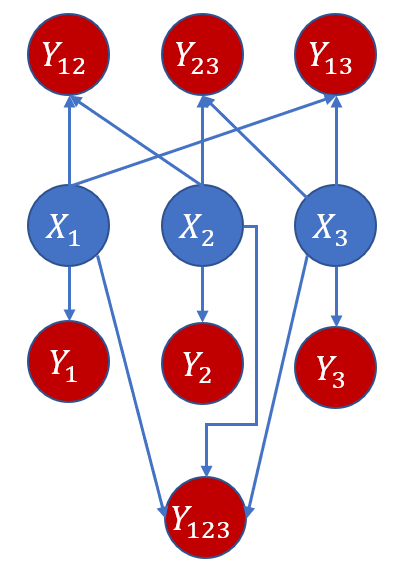
Figure 2. The causal graph where the edges represent causal directions from the cause time series (e.g. $X_{1}$) to the effect time series (e.g. $Y_{1}$). $Y_{ij}$ represents a time series generated by $agg(\{X^{\prime}_{i},X^{\prime}_{j}\})$, where $X_{i}\prec X^{\prime}_{i}$ with some fixed lag $\Delta$.

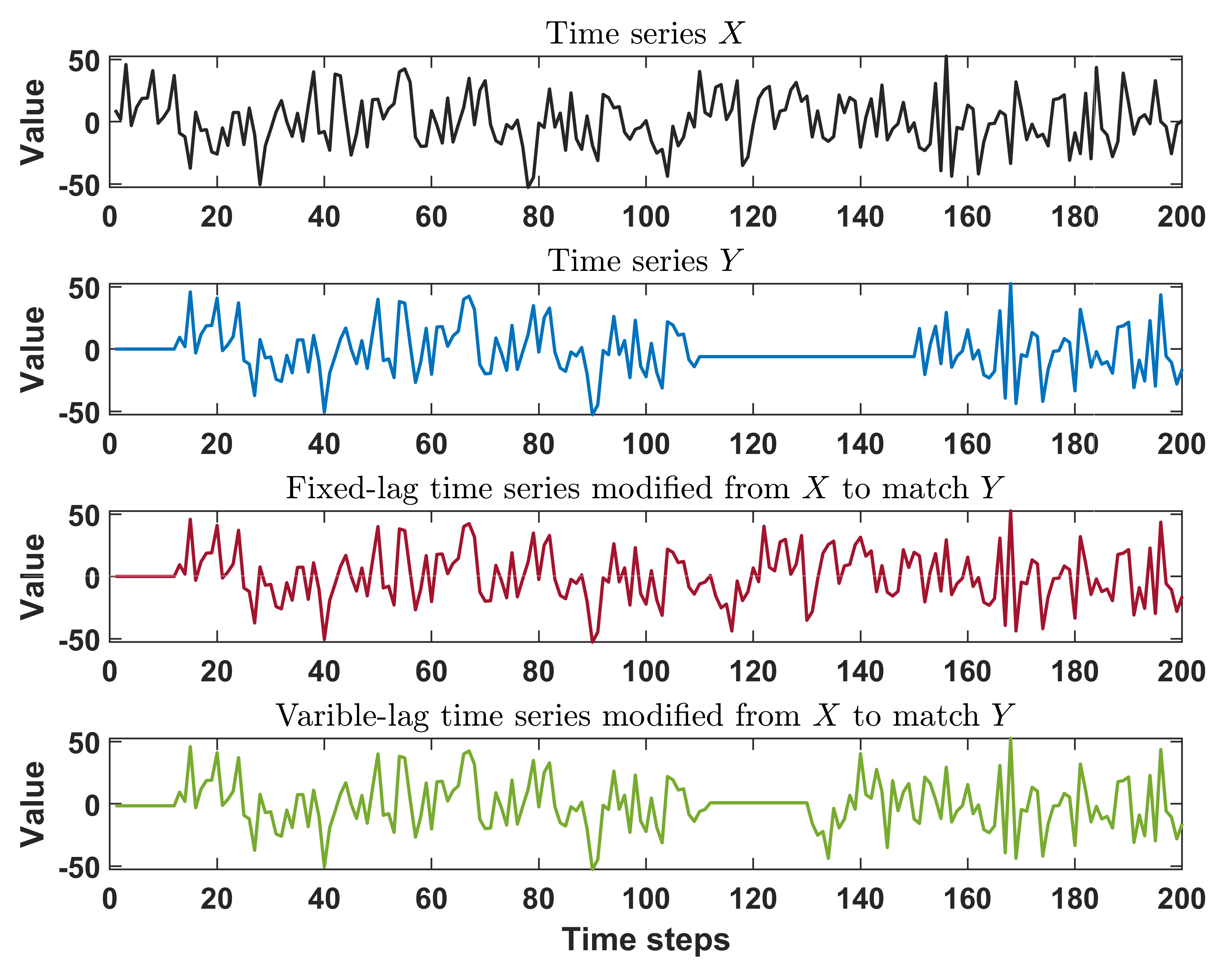
Figure 3. The comparison between the original time series $X$, variable-lag follower $Y$, fixed-lag time series modified from $X$ to match $Y$, and variable-lag time series modified from $X$ to match $Y$. The traditional Granger causality uses only fixed-lag version of $X$ to infer whether $X$ causes $Y$, while our approach uses both versions of $X$ to determine the causality between $X,Y$. Both $X,Y$ are generated from $\mathcal{N}$. $Y$ remains constant from time 110 to 170, which makes it a variable-lag follower of $X$.

See Appendix C for the code we used to generated the datasets.

8.2.3. Schools of fish

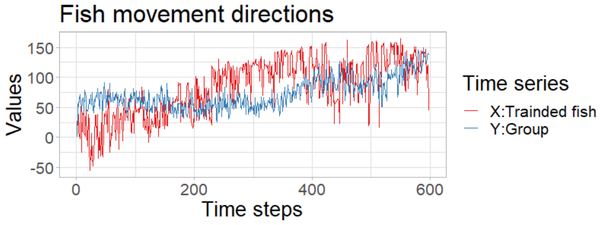
Figure 4. Time series of fish movement: $X$ is an aggregated time series of movement directions of trained fish and $Y$ is an aggregated time series of movement directions of untrained fish, which is the rest of the group.

We used the dataset of golden shiners (Notemigonus crysoleucas) that is publiclly available. The dataset has been collected for the study of information propagation over the visual fields of fish (Strandburg-Peshkin and et al., 2013). A coordination event consists of two-dimensional time series of fish movement that are recorded by video. The time series of fish movement are around 600 time steps. The number of fish in each dataset is around 70 individuals, of which 10 individuals are “informed” fish who have been trained to go to a feeding site. Trained fish lead the group to feeding sites while the rest of the fish just follow the group. We represent the dataset as a pair of aggregated time series: $X$ being the aggregated time series of the directions of trained fish and $Y$ being the aggregated time series of the directions of untrained fish (see Fig. 4). The task is to infer whether $X$ (trained fish) is a cause of $Y$ (the rest of the group).

8.2.4. Troop of baboons

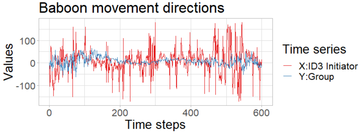
Figure 5. Time series of baboon movement: $X$ is a time series of movement directions of ID3 and $Y$ is an aggregated time series of movement directions of the rest of the group.

We used another publicly available dataset of animal behavior, the movement of a troop of olive baboons (Papio anubis). The dataset consists of GPS tracking information from 26 members of a troop, recorded at 1 Hz from 6 AM to 6 PM between August 01, 2012 and August 10, 2012. The troop lives in the wild at the Mpala Research Centre, Kenya (Crofoot et al., 2015; Strandburg-Peshkin et al., 2015). For the analysis, we selected the 16 members of the troop that have GPS information available for 10 consecutive days, with no missing data. We selected a set of trajectories of lat-long coordinates from a highly coordinated event that has the length of 600 time steps (seconds) for each baboon. This known coordination event is on August 02, 2012 in the morning, with the baboon ID3 initiating the movement, followed by the rest of the troop (Amornbunchornvej et al., 2018). Again, the goal is to infer ID3 (time series $X$) as the cause of the movement of the rest of the group (aggregate time series $Y$) (see Fig. 5).

8.2.5. Gas furnace

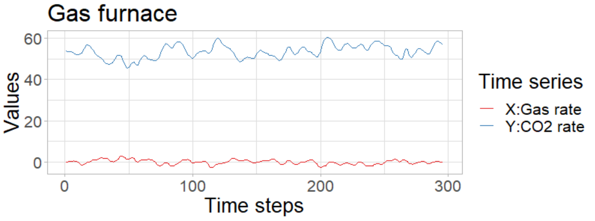
Figure 6. Time series of Gas furnace: $X$ is time series of gas consumption rate and $Y$ is time series of $CO_{2}$.

This dataset consists of information regarding a gas consumption by a gas furnace (Box et al., 2015). $X$ is time series of gas consumption rate and $Y$ is time series of $CO_{2}$ rate produced by a gas furnace (see Fig. 6). Both $X,Y$ have 296 time steps.

8.2.6. Old Faithful geyser eruption

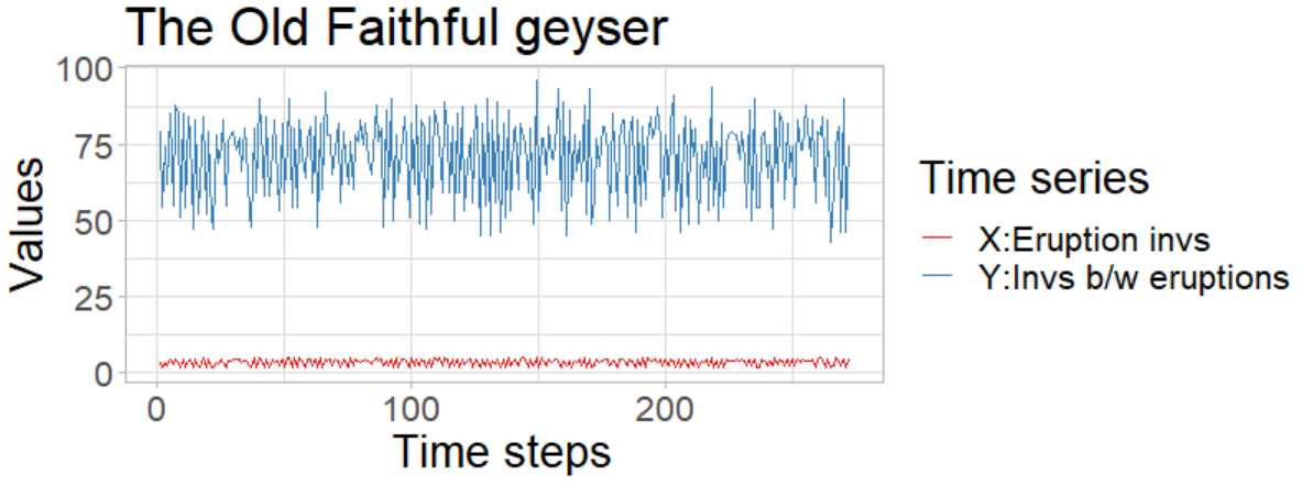
Figure 7. Time series of the Old Faithful geyser eruption: $X$ is time series of eruption intervals and $Y$ is time series of the intervals between current eruption and the next eruption.

This dataset consists of information regarding eruption durations and intervals between eruption events at Old Faithful geyser (Azzalini and Bowman, 1990). $X$ is time series of eruption duration and $Y$ is time series of the interval between current eruption and the next eruption (see Fig. 7). Both $X,Y$ have 298 time steps.

8.3. Time complexity and running time

Table 2. Running time of our approaches with varying time series length $T$ and maximum time delay $\delta_{max}$.

	VL-G		VL-TE
$\delta_{max}/T$	$T=5000$	$T=20000$	$T=5000$	$T=20000$
0.05	5.39	110.00	17.57	126.02
0.10	7.90	128.19	17.42	121.38
0.20	9.22	200.17	17.93	131.23

The main cost of computation in our approach is DTW. We used the “Windowing technique” for the search area of warping  (Keogh and Pazzani, 2001). The main parameter for windowing technique is the maximum time delay $\delta_{max}$. Hence, the time complexity of VL-G is $\mathcal{O}(T\delta_{max})$. The time complexity of TE can be at most $\mathcal{O}(T^{3})$ (Shao et al., 2014), which makes VL-TE has the same time complexity. However, with the work by Kontoyiannis and Skoularidou in (Kontoyiannis and Skoularidou, 2016), the convergence rate of TE approximation can be reduced to $\mathcal{O}(1/\sqrt{T})$ if time series are generated with a Markov-chain property of a given lags. Table 2 shows the running time of our approach on time series with the varying length ($T\in\{5000,20000\}$) and maximum time delay ($\delta_{max}\in\{0.05T,0.1T,0,2T\}$).

9. Results

We report the results of our proposed approaches and other methods on both synthetic and real-world datasets. We also explore how the performance of the methods depends on the basic parameter, $\delta_{\max}$.

9.1. Synthetic data: pairwise level

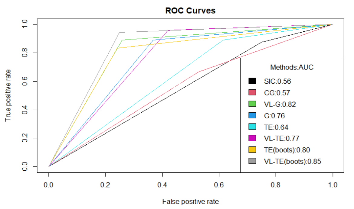
Figure 8. The ROC curves from the results of prediction using pairwise-level simulation datasets.

Figure 8 shows the ROC curves from the results of inferring causal relations and directions. According to the AUC values, all variable-lag methods perform better than their original methods (e.g. VL-G vs. G, VL-TE vs. TE).

The result also shows that our method, VL-Transfer entropy with bootstrapping, VL-TE (boots), performed better than the rest of other methods. The second best method is VL-Granger causality (VL-G), which has the AUC value almost the same as VL-TE (boots). For transfer entropy results, the bootstrapping methods (both VL-TE (boots) and TE (boots) ), performed better than their original version. This indicates that the bootstrapping approach increases the performance of transfer entropy methods in this task.

Moreover, we also investigated the sensitivity of varying the value of the $\delta_{max}$ parameter for all methods. We aggregated the accuracy of inferring causal direction from various cases that have the same $\delta_{max}$ value and report the result. The result in Fig. 9 shows that VL-TE (boots), VL-G, TE (boots), and G can maintain the high accuracy (¿0.9) throughout the range of the values of $\delta_{max}$.

Figure 9. Average accuracy of inferring causal direction as a function of $\delta_{max}$. $x$-axis represents the value of $\delta_{max}$ as a fraction of the time series length $T$ and $y$-axis is the average accuracy.

9.2. Synthetic data: group level

Table 3 shows the result of causal graph inference. The VL-G performed the best overall with the highest F1 score. This result reflects the fact that our approaches can handle complicated time series in causal inference task better than the rest of other methods. VL-TE also performed better than TE.

In addition, we aggregated $X=agg(\{X_{1},X_{2},X_{3}\})$ and $Y=agg(\{Y_{1},Y_{2},\dots,Y_{123}\})$, then we measured the ability of methods to infer that $X$ is a cause of $Y$. The results, which are in the “Group: $X\prec Y$” column in Table 3, show that G, CG and SIC performed well in this task, while the rest of methods failed to infer causal relations. Note that VL-G also performed well when we relaxed the $\gamma$ from 0.3 to 0.01. This is due to the fact that the aggregated group time series have a complicated casual relation between $X=agg(\{X_{1},X_{2},X_{3}\})$ and $Y=agg(\{Y_{1},Y_{2},\dots,Y_{123}\})$, which implies that the causal signal is not strong. Hence, we need to relaxed the $\gamma$ to capture the causal relation.

Comparing transfer entropy methods, the bootstrapping approach decreaseed the performance to detect causal relations compared to their original version. This is also due to the weak signal of causal relation in the complicated datasets.

Overall, the simple original Granger causality performed well in both tasks. Moreover, due to the causal relations in simulation datasets are highly linear, hence, we expect the linear model (e.g. VL-G, G) should perform better than the non-linear approaches (e.g. TE, VL-TE).

Table 3. The results of the precision, recall, and F1-score values of edges inference of causal graph in Fig. 2. Each row is a method and each column is a measure type. The * indicates that the parameter $\gamma$ is changed from 0.3 to 0.01

	Causal graph			Group: $X\prec Y$
Methods	Precision	Recall	F1 score	Accuracy
VL-G	0.93	0.83	0.87	0.23/0.93*
G	0.71	0.99	0.83	0.97
CG	0.04	0.12	0.06	0.90
SIC	0.03	0.11	0.05	0.93
TE	0.17	0.62	0.26	0.50
VL-TE	0.24	0.71	0.35	0.47
TE (boots)	0.08	0.17	0.11	0.30
VL-TE (boots)	0.08	0.18	0.11	0.07

9.3. Real-world datasets

Table 4. The result of inferring causal relations in real-world datasets. Each row is a dataset and each column is a method. An element is one if a method successfully inferred a causal relation with some parameter, while an element is zero if no parameter setting in a method can be used to successfully inferred a causal relation. For VL-G, we used both BIC difference ratio and F-test to infer causal relation. The * implies that VL-G with BIC difference ratio failed to detect causal relations but VL-G with F-test successfully detect the relations. For fish and baboon datasets, VL-G with both criteria were able to detect causal relations.

	Methods
Case	VL-G	G	CG	SIC	TE	VL-TE	TE (boots)	VL-TE (boots)
Fish	1	0	1	0	1	1	0	0
Baboon	1	1	1	1	1	1	0	0
Gas furnace	1*	1	0	1	1	1	1	0
Old faithful geyser	1*	0	1	1	0	1	0	0

Table 4 shows results of inferring causal relations in real-world datasets. For VL-G, it performed better than G. However, BIC difference ratio failed to infer causal relations of gas furnace and old faithful geyser datasets but F-test successfully inferred causal relations in all datasets. Typically, a causal relation that has a high BIC difference ratio can also be detected to have a causal relation by F-test but not vise versa. This suggests that gas furnace and old faithful geyser have weak causal relations. For G, the method cannot detect fish and Old faithful geyser datasets. This suggests that both datasets have a high-level of variable lags that a fixed-lag assumption in G has an issue. For CG, SIC, and TE, they failed in one dataset each. This implies that some dataset that a specific approach failed to detect a causal relation has broke some assumption of a specific approach. Lastly, VL-TE was able to detect all causal relations.

For the old faithful geyser dataset, both G and TE failed to detect a causal relation while both VL-G and VL-TE successfully inferred a causal relation. This implies that this dataset has a high-level of variable lags that broke a fix-lag assumption of G and TE.

Lastly, the transfer entropy methods with bootstrapping almost failed to detect anything. This is due to the weak signal of causal relations in real-world datasets.

9.4. Variable lags vs. fixed lag

9.4.1. VL-Granger causality

To compare the performance of VL-G and G, we simulated 100 datasets of $X\prec Y$ with variable lags. Since $X\prec Y$, a higher BIC difference ratio implies a better result. Fig. 10 shows the results of BIC difference ratio for VL-G and G. Obviously, VL-G has a higher BIC difference ratio than G’s. This suggests that VL-G was able to capture stronger signal of $X$ causes $Y$.

Figure 10. Empirical distributions of BIC difference ratios of VL-Granger and Granger methods inferred from simulation data of $X\prec Y$. Higher BIC difference ratio implies better model if $X$ is the cause of $Y$.

9.4.2. VL-Transfer Entropy

To compare the performance of VL-TE and TE, we also simulated 100 datasets of $X\prec Y$ with variable lags. Since $X\prec Y$, a higher transfer entropy ratio implies a better result. Fig. 11 shows the results of transfer entropy ratio for VL-TE and TE. Obviously, VL-TE has a higher transfer entropy ratio than TE’s. This suggests that VL-TE was able to capture stronger signal of $X$ causes $Y$.

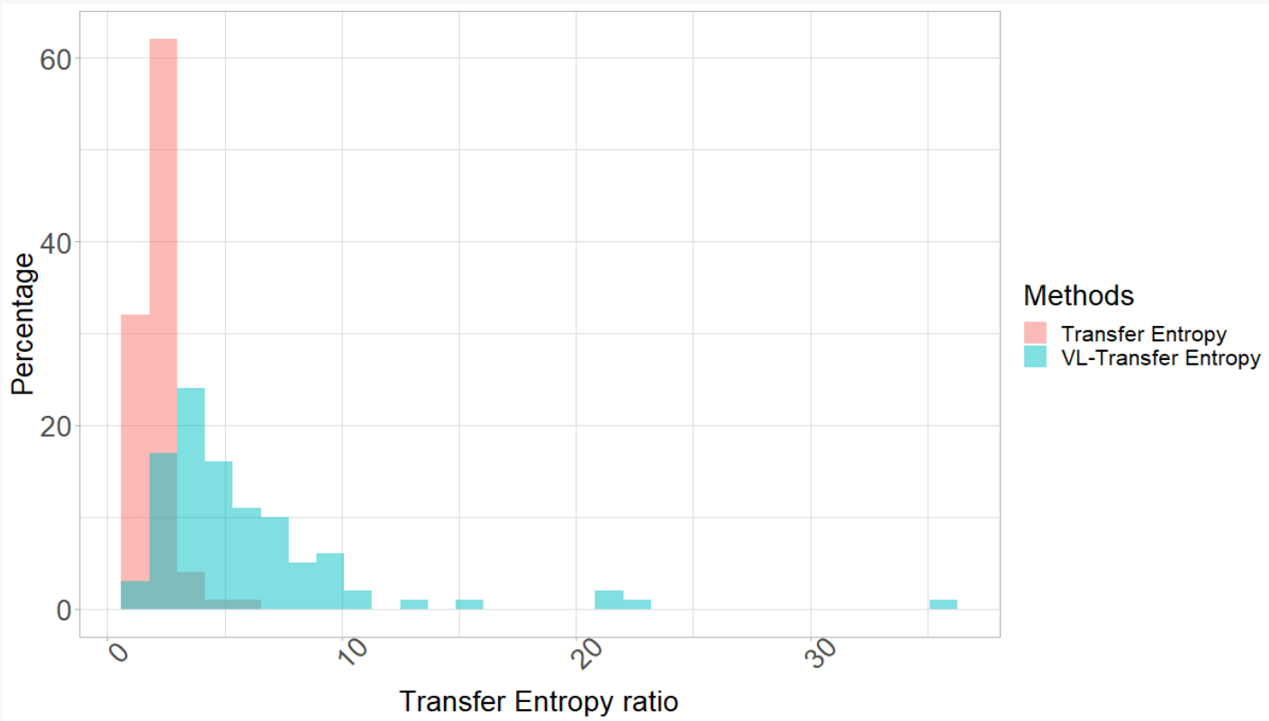
Figure 11. Empirical distributions of transfer entropy ratios of VL-transfer entropy and transfer entropy methods inferred from simulation data of $X\prec Y$. Higher transfer entropy ratio implies better model if $X$ is the cause of $Y$.

10. Conclusions

In this work, we proposed a method to infer Granger and transfer entropy causal relations in time series where the causes influence effects with arbitrary time delays, which can change dynamically. We formalized a new Granger causal relation and a new transfer entropy causal relation, proving that they are true generalizations of the traditional Granger causality and transfer entropy respectively. We demonstrated on both carefully designed synthetic datasets and noisy real-world datasets that the new causal relations can address the arbitrary-time-lag influence between cause and effect, while the traditional Granger causality and transfer entropy cannot. Moreover, in addition to improving and extending Granger causality and transfer entropy, our approach can be applied to infer leader-follower relations, as well as the dependency property between cause and effect. Note that, in simulation datasets, we did not include nonlinear datasets in our analysis. We expect that the linear measures (e.g. VL-Granger and Granger) should outperform the non-linear measures (Transfer Entropy and VL-Transfer Entropy) in the linear datasets, while the non-linear measures should outperform linear measures in non-linear datasets.

We have shown that, in many situations, the causal relations between time series do not have a lock-step connection of a fixed lag that the traditional Granger causality and transfer entropy assume. Hence, traditional Granger causality and transfer entropy missed true existing causal relations in such cases, while our methods correctly inferred them. Our approach can be applied in any domain of study where the causal relations between time series is of interest. The R-CRAN package entitled VLTimeCausality is provided at (Amornbunchornvej, [n. d.]). See Appendix B for the example of how to use the package.

Appendix A Appendix: Dynamic time warping

The Dynamic Time Warping (DTW) (Sakoe and Chiba, 1978) is one of well-known distance measures between a pairwise of time series. The main idea of DTW is to compute the distance from the matching of similar elements between time series. The series of indices of matching is called “Warping path”. Given time series $X,Y$ that have length $T_{X}$ and $T_{Y}$ respectively, their warping path is defined as $P=(\Delta_{1},\dots,\Delta_{K})$ where the following conditions are true (Keogh and Pazzani, 2001):

• $\Delta_{1}=(1,1)$,

• $\Delta_{K}=(T_{X},T_{Y})$,

• $\max(\{T_{X},T_{Y}\})\leq K<T_{X}+T_{Y}-1$ and

• for all pair $\Delta_{t-1}=(i^{\prime},j^{\prime}),\Delta_{t}=(i,j)$, we have $\Delta_{t-1}\in\{(i-1,j),(i,j-1),(i-1,j-1)\}$ where $i^{\prime}\geq 1$ and $j^{\prime}\geq 1$.

Each $\Delta=(i,j)$ in $P$ represents the matching indices where $X(i)$ is matched with $Y(j)$. Suppose $\mathbb{P}$ is a set of all possible warping paths that satisfy the conditions above, the following equation represents the DTW distance between $X,Y$.

(16) $$d_{DTW}=\min_{P\in\mathbb{P}}\sum_{\Delta_{t}\in P,\Delta_{t}=(i,j)}D(i,j).$$

Where $D(i,j)$ is a distance function between $X(i),Y(j)$. If we use the Euclidean distance, then $D(i,j)=\sqrt{X(i)^{2}+Y(j)^{2}}$. A warping path $P^{*}$ that minimizes the Eq. 16 is called an “optimal warping path”. The Eq. 16 solution can be solved by the dynamic programming technique. In the the dynamic programming, given $\mathcal{D}(i,j)$ as a DTW distance of time series $X$ within the interval $[1,i]$, and time series $Y$ within the interval $[1,j]$, we can use the following equation to compute $\mathcal{D}(i,j)$ (Senin, 2008).

(17) $$\mathcal{D}(i,j)=\left\{\begin{array}[]{@{}ll@{}}D(i,j),&i=1,j=1\\ \mathcal{D}(i,j-1)+D(i,j),&i=1,j>1\\ \mathcal{D}(i-1,j)+D(i,j),&i>1,j=1\\ D(i,i)+\min(\{\mathcal{D}(i-1,j),\mathcal{D}(i,j-1),\mathcal{D}(i-1,i-1)\}),&\mathrm{Otherwise}.\end{array}\right.$$

For time series $X,Y$, our goal is to compute the DTW distance $d_{DTW}=\mathcal{D}(T_{X},T_{Y})$, of which its solution can be founded using the Algorithm 5.

input :  Time series $X,Y$ that have length $T_{X}$ and $T_{Y}$ respectively.

output :  $T_{X}\times T_{Y}$-Matrix $\mathcal{D}$, the DTW distance $d_{DTW}$, and DTW optimal warping path $P$.

1 Let $D$ be a $T_{X}\times T_{Y}$-Matrix matrix of Euclidean distances of elements $X$ and $Y$ s.t. $D(i,j)=\sqrt{X(i)^{2}+Y(j)^{2}}$;

2 Set $\mathcal{D}(1,1)=D(1,1)$;

3 for $t=2\to T_{X}$ do

       $\mathcal{D}(t,1)=\mathcal{D}(t-1,1)+D(t,1)$;

      

end for

4for $t=2\to T_{Y}$ do

       $\mathcal{D}(1,t)=\mathcal{D}(1,t-1)+D(1,t)$;

      

end for

5for $t_{X}=2\to T_{X}$ do

      6 for $t_{Y}=2\to T_{Y}$ do

            7 $\mathcal{D}(t_{X},t_{Y})=D(t_{X},t_{Y})+\min(\{\mathcal{D}(t_{X}-1,t_{Y}),\mathcal{D}(t_{X},t_{Y}-1),\mathcal{D}(t_{X}-1,t_{Y}-1)\})$;

            

       end for

      

end for

8$d_{DTW}=\mathcal{D}(T_{X},T_{Y})$;

9 $P^{*}$=WarpingPathFindingFunction($\mathcal{D}$);

10 Return $\mathcal{D},d_{DTW},P^{*}$;

Algorithm 5 DTWFunction

In Algorithm 5 line 1, we compute Euclidean distance for all pair $X(i),Y(j)$ and keep the result in $D(i,j)$. Then, in the line 2-4, we compute the base-case distance ($\mathcal{D}(1,1)=D(1,1)$), and accumulated distances around the marginal areas of the matrix $\mathcal{D}$. In the line 5-8, we use Eq. 17 to compute $\mathcal{D}(i,j)$. The $d_{DTW}$ is reported at the line 9. In the line 10, we infer the optimal warping path by backtracking the steps from $\mathcal{D}(T_{X},T_{Y})$ to $\mathcal{D}(1,1)$ using the Algorithm 6.

input :  $T_{X}\times T_{Y}$-Matrix $\mathcal{D}$.

output :  DTW optimal warping path $P^{*}$.

1Set $P^{\prime}(1)=(T_{X},T_{Y})$, $k=1$, and $\Delta^{*}=(T_{X},T_{Y})$;

2 while $\Delta^{*}\neq(1,1)$ do

      3 Let $(i,j)=P^{\prime}(k)$ and $\mathcal{D}(a)=\mathcal{D}(a_{1},a_{2})$ where $a=(a_{1},a_{2})$ ;

      4 Let $I\subseteq\{(i-1,j),(i-1,j-1),(i,j-1)\}$ s.t. $\forall(k,l)\in I,k\geq 1,l\geq 1$;

      5 $\Delta^{*}=\operatorname*{\mathop{\mathrm{argmin}}\limits}_{\Delta\in I}\mathcal{D}(\Delta)$;

      6 $P^{\prime}(k+1)=\Delta^{*}$;

      7 $k=k+1$;

      

end while

8Let $P^{\prime}$ have a length $K$;

9 Let $P^{*}$ be the optimal warping path with length $K$ where $\forall i\in\{1,\dots,K\},P^{*}(i)=P^{\prime}(K-i+1)$;

10 Return $P^{*}$;

Algorithm 6 WarpingPathFindingFunction

In Algorithm 6, starting at the cell $\mathcal{D}(T_{X},T_{Y})$ (line 1), we search for the neighbor cell in $\mathcal{D}$ that have the lowest accumulative distance ($\Delta^{*}=\operatorname*{\mathop{\mathrm{argmin}}\limits}_{\Delta\in I}\mathcal{D}(\Delta)$). Then, we mark the minimum-distance neighbor cell ($P^{\prime}(k+1)=\Delta^{*}$) as well as jumping to the marked cell ($k=k+1$) and continue for the next iteration (line 2-6). We repeat the steps of marking the minimum-distance neighbor cell until we meet the $\mathcal{D}(1,1)$ cell. The list of all marked cells is the optimal warping path ($P^{*}$).

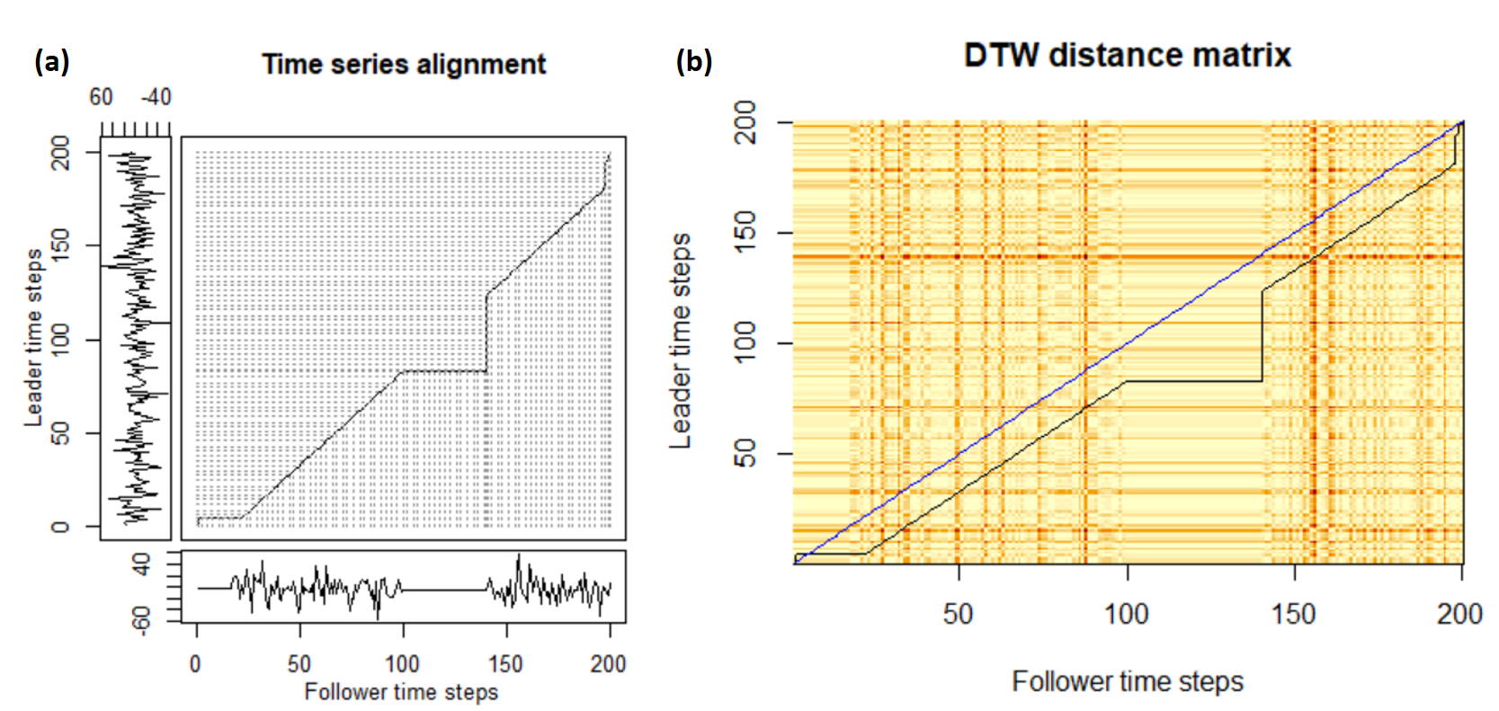
Figure 12. The example of time series alignment by DTW. In this example, the follower time series imitates the leader with time delay $17$ time steps. Between 110th and 150th time steps, the follower constantly imitates leader at the 83th time step. (a) The matching between elements of follower time series and elements of leader time series. The black line is the optimal warping path. (b) The heatmap of accumulative distance matrix $\mathcal{D}$ of DTW and the optimal warping path (black line) compared against the diagonal line (blue line). A darker color represents a higher distance.

Figrue 12 illustrates the example of DTW matching between two time series. In this example, the follower time series imitates the leader with time delay $17$ time steps. Then between 110th and 150th time steps, the follower constantly imitates leader at the 83th time step. The Figure 12 (a) shows the matching of elements between time series. The black line is the optimal warping path. We can see that, in the optimal warping path, the elements between 110th and 150th time steps of follower time series matched with the element of leader at the 83th time step. The Figure 12 (b) shows the DTW accumulative distance matrix $\mathcal{D}$. The optimal warping path is in the black color, while the blue line is a diagonal line of the matrix. A darker color represents a higher distance. We can see that the optimal warping path is below the diagonal line. This implies that the follower elements are matched with the leader elements back in time. Specifically, for any pair of indices $(i,j)$ within the optimal warping path, $\Delta=j-i>0$, when the optimal warping path is below the diagonal line. The element $Y(j)$ is matched with $X(i)$ in the past. Hence, we can infer whether $X\prec Y$ using their optimal warping path.

Appendix B Appendix: VLTimeCausality package

The VLTimeCausality package contains the implementation of VL-Granger causality, Granger causality, and VL-Transfer entropy. The package is available on the the Comprehensive R Archive Network (CRAN). This implies all R programming users can install our package anywhere. To install the package, we can use the following commands.

⬇

1R>install.packages("VLTimeCausality")

To use the package, the first step is to use the provided function to generate simulation time series.

⬇

1R>library(VLTimeCausality)

2R>TS <- VLTimeCausality::SimpleSimulationVLtimeseries()

The TS variable contains TS$X and TS$Y where TS$X causes TS$Y. Then, we can run VL-Granger causality with the $\gamma=0.5$ below.

⬇

1R>out<-VLTimeCausality::VLGrangerFunc(Y=TS$Y,X=TS$X, gamma= 0.5)

The result of inference is below.

⬇

1R> out$XgCsY

2[1] TRUE

3R> out$BICDiffRatio

4[1] 0.8434518

It implies that TS$X causes TS$Y (out$XgCsY is true) with the BIC difference ratio at 0.84.

For the VL-Transfer Entropy, the following command is used to check whether TS$X causes TS$Y with the number of bootstrap replicates is 100 and the significance level $\alpha=0.05$.

⬇

1R> out2<-VLTransferEntropy(Y=TS$Y,X=TS$X,VLflag=TRUE,nboot=100, alpha = 0.05)

The result of inference is below.

⬇

1R> out2$XgCsY_trns

2[1] TRUE

3R> out2$TEratio

4[1] 4.539785

5R> out2$pval

6[1] 0

It implies that TS$X causes TS$Y (out2$XgCsY_trns is true) with the transfer entropy ratio at 4.54 and the p-value is at 0. For more details about functions and parameters in the packages, please see https://cran.r-project.org/package=VLTimeCausality.

Appendix C Appendix: Simulation generating code

The following code was used to generate simulation datasets that were analyzed and reported the results in Section 9.1. We deployed the “rmatio” package (Widgren and Hulbert, 2019) for files operation handling. Although our simulation datasets were generated randomly, we set the random seeds to make it being able to be replicated.

⬇

1library(rmatio)

2library(VLTimeCausality)

3origSeed<-2020

4set.seed(origSeed)

5rounds<-15

6seeds<-runif(rounds,1000,250000)

7simType1DataSets<-list()

8

9# normal gen

10for(i in seq(rounds))

11{

12 simType1DataSets[["normalPos"]][[i]]<- SimpleSimulationVLtimeseries(expflag = FALSE, arimaFlag = FALSE,causalFlag = TRUE, seedVal = seeds[i] )

13 simType1DataSets[["normalNeg"]][[i]]<- SimpleSimulationVLtimeseries(expflag = FALSE, arimaFlag = FALSE,causalFlag = FALSE, seedVal = seeds[i] )

14

15 simType1DataSets[["ARMAPos"]][[i]]<- SimpleSimulationVLtimeseries(expflag = FALSE, arimaFlag = TRUE,causalFlag = TRUE, seedVal = seeds[i] )

16 simType1DataSets[["ARMANeg"]][[i]]<- SimpleSimulationVLtimeseries(expflag = FALSE, arimaFlag = TRUE,causalFlag = FALSE, seedVal = seeds[i] )

17

18 simType1DataSets[["normalARMANeg"]][[i]]<- simType1DataSets[["normalNeg"]][[i]]

19 simType1DataSets[["normalARMANeg"]][[i]]$Y<-simType1DataSets[["ARMANeg"]][[i]]$Y

20

21}

22simType1DataSets$origSeed<-origSeed

23simType1DataSets$seeds<-seeds

24simType1DataSets$rounds<-rounds

25write.mat(file = "simType1DataSets.mat",object = simType1DataSets)

The following code was used to generate simulation datasets that were analyzed and reported the results in Section 9.2.

⬇

1library(rmatio)

2library(VLTimeCausality)

3origSeed<-2020

4set.seed(origSeed)

5rounds<-15

6seeds<-runif(rounds,1000,250000)

7simType2DataSets<-list()

8

9# normal gen

10for(i in seq(rounds))

11{

12

13 TS<- MultipleSimulationVLtimeseries(seedVal = seeds[i], arimaFlag = FALSE)

14 simType2DataSets[["normal"]][[i]]<-TS

15 simType2DataSets[["normalX"]][[i]]<-rowMeans(TS[,1:3])

16 simType2DataSets[["normalY"]][[i]]<-rowMeans(TS[,4:10])

17

18

19 TS<- MultipleSimulationVLtimeseries(seedVal = seeds[i], arimaFlag = TRUE)

20 simType2DataSets[["ARMA"]][[i]]<-TS

21 simType2DataSets[["ARMAX"]][[i]]<-rowMeans(TS[,1:3])

22 simType2DataSets[["ARMAY"]][[i]]<-rowMeans(TS[,4:10])

23

24}

25simType2DataSets$origSeed<-origSeed

26simType2DataSets$seeds<-seeds

27simType2DataSets$rounds<-rounds

28write.mat(file = "simType2DataSets.mat",object = simType2DataSets)

References

- (1)
- MLS ([n. d.]) [n. d.]. Granger Causality Package in MATLAB. https://www.mathworks.com/matlabcentral/fileexchange/25467-granger-causality-test.
- RSo ([n. d.]) [n. d.]. Granger Causality Package in R. https://www.rdocumentation.org/packages/MSBVAR/versions/0.9-2/topics/granger.test.
- Amornbunchornvej ([n. d.]) Chainarong Amornbunchornvej. [n. d.]. VLTimeSeriesCausality: R package for variable-lag causal inference in time series. https://github.com/DarkEyes/VLTimeSeriesCausality. Accessed: 2019-12-10.
- Amornbunchornvej et al. (2018) Chainarong Amornbunchornvej, Ivan Brugere, Ariana Strandburg-Peshkin, Damien Farine, Margaret C Crofoot, and Tanya Y Berger-Wolf. 2018. Coordination Event Detection and Initiator Identification in Time Series Data. ACM Trans. Knowl. Discov. Data 12, 5, Article 53 (6 2018), 33 pages. https://doi.org/10.1145/3201406
- Amornbunchornvej et al. (2019) Chainarong Amornbunchornvej, Elena Zheleva, and Tanya Berger-Wolf. 2019. Variable-lag Granger Causality for Time Series Analysis. In 2019 IEEE International Conference on Data Science and Advanced Analytics (DSAA). IEEE, 21–30. https://doi.org/10.1109/DSAA.2019.00016
- Arnold et al. (2007) Andrew Arnold, Yan Liu, and Naoki Abe. 2007. Temporal Causal Modeling with Graphical Granger Methods. In Proceedings of the 13th ACM SIGKDD International Conference on Knowledge Discovery and Data Mining (KDD ’07). ACM, New York, NY, USA, 66–75. https://doi.org/10.1145/1281192.1281203
- Atukeren et al. (2010) Erdal Atukeren et al. 2010. The relationship between the F-test and the Schwarz criterion: implications for Granger-causality tests. Econ Bull 30, 1 (2010), 494–499.
- Azzalini and Bowman (1990) Adelchi Azzalini and Adrian W Bowman. 1990. A look at some data on the Old Faithful geyser. Journal of the Royal Statistical Society: Series C (Applied Statistics) 39, 3 (1990), 357–365.
- Barnett et al. (2009) Lionel Barnett, Adam B. Barrett, and Anil K. Seth. 2009. Granger Causality and Transfer Entropy Are Equivalent for Gaussian Variables. Phys. Rev. Lett. 103 (Dec 2009), 238701. Issue 23. https://doi.org/10.1103/PhysRevLett.103.238701
- Behrendt et al. (2019) Simon Behrendt, Thomas Dimpfl, Franziska J. Peter, and David J. Zimmermann. 2019. RTransferEntropy — Quantifying information flow between different time series using effective transfer entropy. SoftwareX 10 (2019), 100265. https://doi.org/10.1016/j.softx.2019.100265
- Box et al. (2015) George EP Box, Gwilym M Jenkins, Gregory C Reinsel, and Greta M Ljung. 2015. Time series analysis: forecasting and control. John Wiley & Sons.
- Chazelle (2011) Bernard Chazelle. 2011. The Total s-Energy of a Multiagent System. SIAM Journal on Control and Optimization 49, 4 (2011), 1680–1706. https://doi.org/10.1137/100791671 arXiv:https://doi.org/10.1137/100791671
- Chen et al. (2004) Yonghong Chen, Govindan Rangarajan, Jianfeng Feng, and Mingzhou Ding. 2004. Analyzing multiple nonlinear time series with extended Granger causality. Physics Letters A 324, 1 (2004), 26–35.
- Crofoot et al. (2015) Margaret C Crofoot, Roland W Kays, and Martin Wikelski. 2015. Data from: Shared decision-making drives collective movement in wild baboons.
- Dimpfl and Peter (2013) Thomas Dimpfl and Franziska Julia Peter. 2013. Using transfer entropy to measure information flows between financial markets. Studies in Nonlinear Dynamics & Econometrics 17, 1 (2013), 85–102.
- Eichler (2013) Michael Eichler. 2013. Causal inference with multiple time series: principles and problems. Philosophical Transactions of the Royal Society A: Mathematical, Physical and Engineering Sciences 371, 1997 (2013), 20110613. https://doi.org/10.1098/rsta.2011.0613
- Giorgino et al. (2009) Toni Giorgino et al. 2009. Computing and visualizing dynamic time warping alignments in R: the dtw package. Journal of statistical Software 31, 7 (2009), 1–24.
- Granger and Jeon (2004) Clive Granger and Yongil Jeon. 2004. Forecasting performance of information criteria with many macro series. Journal of Applied Statistics 31, 10 (2004), 1227–1240.
- Granger (1969) Clive WJ Granger. 1969. Investigating causal relations by econometric models and cross-spectral methods. Econometrica: Journal of the Econometric Society (1969), 424–438.
- Griveau-Billion and Calderhead (2019) Théophile Griveau-Billion and Ben Calderhead. 2019. Efficient structure learning with automatic sparsity selection for causal graph processes. arXiv preprint arXiv:1906.04479 (2019).
- Iseki et al. (2019) Akane Iseki, Y. Mukuta, Y. Ushiki, and T. Harada. 2019. Estimating the causal effect from partially observed time series. In AAAI.
- Janzing and Scholkopf (2010) Dominik Janzing and Bernhard Scholkopf. 2010. Causal inference using the algorithmic Markov condition. IEEE Transactions on Information Theory 56, 10 (2010), 5168–5194.
- Keogh and Pazzani (2001) Eamonn J Keogh and Michael J Pazzani. 2001. Derivative dynamic time warping. In Proceedings of the 2001 SIAM international conference on data mining. SIAM, 1–11.
- Kontoyiannis and Skoularidou (2016) Ioannis Kontoyiannis and Maria Skoularidou. 2016. Estimating the directed information and testing for causality. IEEE Transactions on Information Theory 62, 11 (2016), 6053–6067.
- Lee et al. (2012) Joon Lee, Shamim Nemati, Ikaro Silva, Bradley A Edwards, James P Butler, and Atul Malhotra. 2012. Transfer entropy estimation and directional coupling change detection in biomedical time series. Biomedical engineering online 11, 1 (2012), 19.
- Liu et al. (2012) Yan Liu, Taha Bahadori, and Hongfei Li. 2012. Sparse-gev: Sparse latent space model for multivariate extreme value time serie modeling. In ICML.
- Malinsky and Spirtes (2018) Daniel Malinsky and Peter Spirtes. 2018. Causal structure learning from multivariate time series in settings with unmeasured confounding. In Proceedings of 2018 ACM SIGKDD Workshop on Causal Discovery. 23–47.
- Mueen and Keogh (2016) Abdullah Mueen and Eamonn Keogh. 2016. Extracting Optimal Performance from Dynamic Time Warping. In Proceedings of the 22Nd ACM SIGKDD International Conference on Knowledge Discovery and Data Mining (KDD ’16). ACM, New York, NY, USA, 2129–2130. https://doi.org/10.1145/2939672.2945383
- Pearl (2000) J Pearl. 2000. Causality: Models, reasoning and inference Cambridge University Press. Cambridge, MA, USA, 9 (2000).
- Peng et al. (2007) Wei Peng, Tong Sun, Philip Rose, and Tao Li. 2007. A Semi-automatic System with an Iterative Learning Method for Discovering the Leading Indicators in Business Processes. In Proceedings of the 2007 International Workshop on Domain Driven Data Mining (DDDM ’07). ACM, New York, NY, USA, 33–42. https://doi.org/10.1145/1288552.1288557
- Peters et al. (2013) Jonas Peters, Dominik Janzing, and Bernhard Schölkopf. 2013. Causal inference on time series using restricted structural equation models. In Advances in Neural Information Processing Systems. 154–162.
- Peters et al. (2017) Jonas Peters, Dominik Janzing, and Bernhard Schölkopf. 2017. Elements of causal inference: foundations and learning algorithms. MIT press.
- Quinn et al. (2015) C. J. Quinn, N. Kiyavash, and T. P. Coleman. 2015. Directed Information Graphs. IEEE Transactions on Information Theory 61, 12 (Dec 2015), 6887–6909. https://doi.org/10.1109/TIT.2015.2478440
- Raffalovich et al. (2008) Lawrence E Raffalovich, Glenn D Deane, David Armstrong, and Hui-Shien Tsao. 2008. Model selection procedures in social research: Monte-Carlo simulation results. Journal of Applied Statistics 35, 10 (2008), 1093–1114.
- Sakoe and Chiba (1978) Hiroaki Sakoe and Seibi Chiba. 1978. Dynamic programming algorithm optimization for spoken word recognition. IEEE transactions on acoustics, speech, and signal processing 26, 1 (1978), 43–49.
- Schölkopf et al. (2012) Bernhard Schölkopf, Dominik Janzing, Jonas Peters, Eleni Sgouritsa, Kun Zhang, and Joris Mooij. 2012. On causal and anticausal learning. In ICML.
- Schreiber (2000) Thomas Schreiber. 2000. Measuring information transfer. Physical review letters 85, 2 (2000), 461.
- Schwab et al. (2019) Patrick Schwab, Djordje Miladinovic, and Walter Karlen. 2019. Granger-causal attentive Mixtures of Experts: Learning Important Features with Neural Networks. In AAAI.
- Senin (2008) Pavel Senin. 2008. Dynamic time warping algorithm review. Information and Computer Science Department University of Hawaii at Manoa Honolulu, USA 855, 1-23 (2008), 40.
- Shajarisales et al. (2015) Naji Shajarisales, Dominik Janzing, Bernhard Schölkopf, and Michel Besserve. 2015. Telling cause from effect in deterministic linear dynamical systems. In ICML. 285–294.
- Shannon (1948) C. E. Shannon. 1948. A mathematical theory of communication. The Bell System Technical Journal 27, 3 (July 1948), 379–423. https://doi.org/10.1002/j.1538-7305.1948.tb01338.x
- Shao et al. (2014) Shengjia Shao, Ce Guo, Wayne Luk, and Stephen Weston. 2014. Accelerating transfer entropy computation. In 2014 International Conference on Field-Programmable Technology (FPT). IEEE, 60–67.
- Shibuya et al. (2009) Takashi Shibuya, Tatsuya Harada, and Yasuo Kuniyoshi. 2009. Causality quantification and its applications: structuring and modeling of multivariate time series. In KDD. ACM.
- Siggiridou and Kugiumtzis (2016) Elsa Siggiridou and Dimitris Kugiumtzis. 2016. Granger causality in multivariate time series using a time-ordered restricted vector autoregressive model. IEEE Transactions on Signal Processing 64, 7 (2016), 1759–1773.
- Sliva et al. (2015) Amy Sliva, Scott Neal Reilly, Randy Casstevens, and John Chamberlain. 2015. Tools for validating causal and predictive claims in social science models. Procedia Manufacturing 3 (2015), 3925–3932.
- Spirtes et al. (1993) Peter Spirtes, Clark Glymour, and Richard Scheines. 1993. Discovery Algorithms for Causally Sufficient Structures. Springer New York, New York, NY, 103–162. https://doi.org/10.1007/978-1-4612-2748-9_5
- Strandburg-Peshkin and et al. (2013) A. Strandburg-Peshkin and et al. 2013. Visual sensory networks and effective information transfer in animal groups. Current Biology 23, 17 (2013), R709–R711.
- Strandburg-Peshkin et al. (2015) Ariana Strandburg-Peshkin, Damien R Farine, Iain D Couzin, and Margaret C Crofoot. 2015. Shared decision-making drives collective movement in wild baboons. Science 348, 6241 (2015), 1358–1361.
- Sun et al. (2015) Youqiang Sun, Jiuyong Li, Jixue Liu, Christopher Chow, Bingyu Sun, and Rujing Wang. 2015. Using causal discovery for feature selection in multivariate numerical time series. Machine Learning 101, 1 (01 Oct 2015), 377–395. https://doi.org/10.1007/s10994-014-5460-1
- Varian (2016) Hal R. Varian. 2016. Causal inference in economics and marketing. Proceedings of the National Academy of Sciences 113, 27 (2016), 7310–7315. https://doi.org/10.1073/pnas.1510479113 arXiv:https://www.pnas.org/content/113/27/7310.full.pdf
- Widgren and Hulbert (2019) Stefan Widgren and Christopher Hulbert. 2019. rmatio: Read and Write ’Matlab’ Files. https://CRAN.R-project.org/package=rmatio R package version 0.14.0.
- Yuan et al. (2016) Tao Yuan, Gang Li, Zhaohui Zhang, and S Joe Qin. 2016. Deep causal mining for plant-wide oscillations with multilevel Granger causality analysis. In American Control Conference (ACC), 2016. IEEE, 5056–5061.