A Novel Massive MIMO Beam Domain
Channel Model

Abstract

A novel beam domain channel model (BDCM) for massive multiple-input multiple-output (MIMO) communication systems has been proposed in this paper. The near-field effect and spherical wavefront are firstly assumed in the proposed model, which is different from the conventional BDCM for MIMO based on the far-field effect and plane wavefront assumption. The proposed novel BDCM is the transformation of an existing geometry-based stochastic model (GBSM) from the antenna domain into beam domain. The space-time non-stationarity is also modeled in the novel BDCM. Moreover, the comparison of computational complexity for both models is studied. Based on the numerical analysis, comparison of cluster-level statistical properties between the proposed BDCM and existing GBSM has shown that there exists little difference in the space, time, and frequency correlation properties for two models. Also, based on the simulation, coherence bandwidths of the two models in different scenarios are almost the same. The computational complexity of the novel BDCM is much lower than the existing GBSM. It can be observed that the proposed novel BDCM has similar statistical properties to the existing GBSM at the cluster-level. The proposed BDCM has less complexity and is therefore more convenient for information theory and signal processing research than the conventional GBSMs.

I Introduction

In wireless communication systems, MIMO technology can greatly enhance the channel capacity [1] and improve the reliability of communication systems without requiring additional bandwidth and power [2]. In recent years, massive MIMO technology has become popular because it can simplify the required signal processing[3] and provide a huge improvement in system performance over traditional MIMO technologies [4].

The wireless channel model is a key metric to analyze the performance of the whole communication systems [5]. Recently, multiple GBSMs have been proposed and reviewed in [6]. Among them, a two-dimensional (2D) non-stationary wideband channel model was proposed in [7], where all scatterers were located on multi-confocal ellipses. It considered the near-field effect and the non-stationarity of massive MIMO channel. In [8], a three-dimensional (3D) non-stationary wideband massive MIMO channel model was proposed, which utilized a virtual link to represent the complicated scattering environment. In [9], the authors proposed a general 3D GBSM for fifth generation (5G) wireless communication systems. It is capable of simulating massive MIMO, millimeter wave (mmWave), vehicle-to-vehicle (V2V), and high-speed train (HST) small-scale fading channels.

However, the complexity of the above-mentioned models is relatively high. Simplified GBSMs or correlation-based stochastic models (CBSMs) may be more applicable for information theory and signal processing research. CBSMs can be divided into classical independent and identically distributed (i.i.d.) Rayleigh fading channel model and correlated channel model [10]. Correlated channel models include the Kronecker-based stochastic model (KBSM) [11], Weichselberger model [12], and virtual channel representation (VCR) [13]. However, these conventional CBSMs did not take the near-field effect and non-stationarity into account, and thus are not suitable for massive MIMO channel modeling.

Recently, the BDCM was first proposed in [14], which transferred the channel model into the angular domain or called beam domain with the far-field assumption. The conventional BDCM was applied to the research of information theory and signal processing, especially in the recent proposed beam division multiple access (BDMA) [14]. However, the conventional BDCM also did not consider the massive MIMO characteristics. A more accurate massive MIMO channel model which is convenient for information theory and signal processing research is therefore needed urgently.

In this paper, we propose a novel BDCM for massive MIMO systems and the major contributions are summarized as follows:

1. The proposed novel BDCM is distinguished from the conventional BDCM by considering the near-field effect, spherical wavefront and space-time non-stationarity for the first time.

2. The novel BDCM transfers an existing GBSM into the beam domain and according to the simulation results, the novel BDCM has the similar statistical properties with the existing GBSM in the cluster-level.

3. By comparing the computational complexity of both models, it is found that the novel BDCM has the lower computational complexity and is more suitable for the research of signal processing and information theory than conventional GBSMs.

The remainder of this paper is organized as follows. An existing 2D non-stationary wideband GBSM is presented in Section II. In section III, the proposed novel BDCM is discussed in details. Section IV shows the statistical property analysis of both two models. Results and discussions are presented in Section V. Conclusions are drawn in Section VI.

II An Existing 2D Non-stationary Wideband GBSM

In this section, we will briefly introduce an existing non-stationary wideband GBSM [7]. The channel is modeled as an $M_{R}\times M_{T}$ complex matrix $\mathbf{H}^{G}(t,\tau)=[h^{G}_{kl}(t,\tau)]_{M_{R}\times M_{T}}$, where $k=1,2,\cdots,M_{R}$ and $l=1,2,\cdots,M_{T}$.

$$\mathbf{H}^{G}(t,\tau)=\sum_{n=1}^{N_{\mathrm{total}}}\mathbf{H}^{G}_{n}(t)\delta(\tau-\tau_{n}).$$ (1)

The elements of the channel matrix $\mathbf{H}^{G}(t,\tau)$ are modeled as

$$[\mathbf{H}^{G}(t,\tau)]_{kl}=h^{G}_{kl}(t,\tau)=\sum_{n=1}^{N_{\mathrm{total}}}h^{G}_{kl,n}(t)\delta(\tau-\tau_{n})$$ (2)

where the channel gain $h^{G}_{kl,n}(t)$ of $\mathrm{Cluster}_{n}$ is modeled as the sum of the line-of-sight (LOS) component and the non-line-of-sight (NLOS) components.

–if $\mathrm{Cluster}_{n}\in\left\{C_{l}^{T}\bigcap C_{k}^{R}\right\}$,

$$h^{G}_{kl,n}(t)= \underbrace{\delta(n-1)\sqrt{\frac{K}{K+1}}e^{j(2\pi f_{kl}^{\text{LOS}}t+\varphi_{kl}^{\text{LOS}})}}_{\text{LOS}}$$

$$+\underbrace{\sqrt{\frac{P_{n}}{K+1}}\lim\limits_{S\rightarrow\infty}\frac{1}{\sqrt{S}}\sum_{i=1}^{S}e^{j(2\pi f_{n,i}t+\varphi_{kl,n,i})}}_{\text{NLOS}}$$ (3)

–if $\mathrm{Cluster}_{n}\notin\left\{C_{l}^{T}\bigcap C_{k}^{R}\right\}$,

$$h^{G}_{kl,n}(t)=0.$$ (4)

The detailed calculations of parameters $f_{kl}^{\text{LOS}},\varphi_{kl}^{\text{LOS}},f_{n,i},$ and $\varphi_{kl,n,i}$ and the space-time non-stationarity of the existing GBSM can be found in [7], and we will not go into details.

III A Novel Massive MIMO BDCM

TABLE I: KEY PARAMETER DEFINITIONS OF THE NOVEL MASSIVE MIMO BDCM.

Parameter	Definition
$\text{Ant}_{l}^{T}(\text{Ant}_{k}^{R})$	transmit antenna $l$ (receive antenna $k$)
$\theta_{m}$	the $m$-th virtual angle sampling NLOS AoAs
$f_{m}$	the Doppler frequency of cluster $m$
$\varphi_{kl,m,i}$	the phase of cluster $m$ between transmit antenna $l$ and receive antenna $k$ via the path $i$
$D_{lm,i}^{T}(D_{km,i}^{R})$	the distance between transmit antenna $l$ (receive antenna $k$) and cluster $m$ via the path $i$
$D_{m,i}^{T}(D_{m,i}^{R})$	the distance between transmit (receive) antenna center and cluster $m$ via the path $i$
$f_{kl}^{BL}$	the LOS Doppler frequency from transmit antenna $l$ to receive antenna $k$
$\varphi_{kl}^{BL}$	the phase of the LOS path from transmit antenna $l$ to receive antenna $k$
$\alpha_{l}^{BL}$	the LOS angle of arrival (AoA) from transmit antenna $l$ to receive antenna center
$D_{kl}^{BL}$	the LOS Distance from transmit antenna $l$ to receive antenna $k$
$D_{l}^{BL}$	the LOS Distance from transmit antenna $l$ to receive antenna center
$\alpha_{v}$	the angle of the mobile station (MS) velocity

The complexity of the existing GBSM is relatively high, which is not suitable for information theory and signal processing research. In view of that, in this section, we propose a novel BDCM to transfer the channel from the antenna domain into beam domain. The key parameter definitions of the novel BDCM are summarized in Table I.

III-A The NLOS Condition

Illustration of the NLOS channel for the novel BDCM is shown in Fig. 1. First, let us sample the AoA of the NLOS channel uniformly distributed in the interval $[-\pi,\pi]$, and achieve the virtual angles $\theta_{m}$ as

$$\theta_{m}\triangleq-\pi+\frac{2\pi m}{M},\quad m=1,\cdots,M$$ (5)

where $M$ is the sampling number of the virtual angles. For the simplicity of the derivation, we assume the sampling number of the virtual angles $M$ is finite, and one direction with a virtual angle $\theta_{m}$ is represented as a beam. The AoD $\phi_{m}$ is dependent on the AoA, which is defined as $\phi_{m}=f(\theta_{m})$ [7].

The NLOS parameters are all dependent on the arrival angles, which are defined as

$$f_{m}= f_{\max}\cos\left(\theta_{m}-\alpha_{v}\right)$$ (6)

$$\varphi_{kl,m,i}= \varphi_{0}+\frac{2\pi}{\lambda}\left[D_{lm,i}^{T}+D_{km,i}^{R}\right].$$ (7)

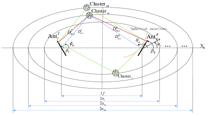
Figure 1: Illustration of the NLOS part for the novel BDCM.

Here, the departure Angles and the arrival Angles of the paths within beam $m$ are approximated as $\phi_{m,i}\approx\phi_{m}$ and $\theta_{m,i}\approx\theta_{m}$, respectively. Moreover, we have

$$D_{lm,i}^{T}= \Big{[}(D_{m,i}^{T})^{2}+\left(\frac{M_{T}-2l+1}{2}\delta_{T}\right)^{2}$$

$$-D_{m,i}^{T}(M_{T}-2l+1)\delta_{T}\cos(\beta_{T}-\phi_{m})\Big{]}$$ (8)

$$D_{km,i}^{R}= \Big{[}(D_{m,i}^{R})^{2}+\left(\frac{M_{R}-2k+1}{2}\delta_{R}\right)^{2}$$

$$-D_{m,i}^{R}(M_{R}-2k+1)\delta_{R}\cos(\theta_{m}-\beta_{R})\Big{]}$$ (9)

where

$$D_{m,i}^{T} =\frac{2a_{m}\sin\phi_{m,i}}{\sin\phi_{m,i}+\sin\theta_{m,i}}$$ (10)

$$D_{m,i}^{R} =\frac{2a_{m}\sin\theta_{m,i}}{\sin\phi_{m,i}+\sin\theta_{m,i}}.$$ (11)

III-B The LOS Condition

Similar but not the same with the existing GBSM, the LOS parameters of the novel BDCM are defined as

$$f_{kl}^{BL}= f_{\max}\cos\Bigg{(}\beta_{R}-\alpha_{v}$$

$$+\arcsin\bigg{[}\frac{D_{l}^{BL}}{D_{kl}^{BL}}\sin\left(\alpha_{l}^{BL}-\beta_{R}\right)\bigg{]}\Bigg{)}$$ (12)

$$\varphi_{kl}^{BL}= \varphi_{0}+\frac{2\pi}{\lambda}D_{kl}^{\text{BL}}$$ (13)

where

$$D_{l}^{BL}= \Big{[}(2f)^{2}+(\frac{M_{T}-2l+1}{2}\delta_{T})^{2}$$

$$-2f(M_{T}-2l+1)\delta_{T}\cos\beta_{T}\Big{]}^{\frac{1}{2}}$$ (14)

$$\alpha_{l}^{BL}= \arcsin\left[\frac{(M_{T}-2l+1)}{2D_{l}^{BL}}\sin\beta_{T}\right]$$ (15)

$$D_{kl}^{BL}= \Bigg{[}(D_{l}^{BL})^{2}+\left(\frac{M_{R}-2k+1}{2}\delta_{R}\right)^{2}$$

$$-(M_{R}-2k+1)\delta_{R}D_{l}^{BL}\cos(\alpha_{l}^{BL}-\beta_{R})\Bigg{]}^{1/2}.$$ (16)

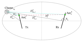
Figure 2: The modeling method of the LOS channel.

The LOS path can be modeled also by utilizing the NLOS paths with the same or similar arrival angles $\theta_{m_{0}}$, which is depicted in Fig. 3, where $m_{0}\in\mathcal{M}=\{1,2,\cdots,M\}$. In this case, the AoA is $\phi_{m_{0}}=f(\theta_{m_{0}})$ [7], and we have the following approximation as

$$D_{kl}^{BL}\approx D_{km_{0},i}^{R}-D_{lm_{0},i}^{T}.$$ (17)

III-C The Whole Channel Model

Based on the virtual angles, we introduce the response vectors as

$$\mathbf{e}_{T}(\theta_{m}) =\left[e_{T}(1;\theta_{m}),\cdots,e_{T}(M_{T};\theta_{m})\right]^{T}$$ (18)

$$\mathbf{e}_{R}(\theta_{m}) =\left[e_{R}(1;\theta_{m}),\cdots,e_{R}(M_{R};\theta_{m})\right]^{T}$$ (19)

where

$$e_{T}(l;\theta_{m}) \triangleq e^{j\frac{2\pi}{\lambda}\left(D_{m,i}^{T}-D_{lm,i}^{T}\right)},\quad l=1,\cdots,M_{T}$$ (20)

$$e_{R}(k;\theta_{m}) \triangleq e^{j\frac{2\pi}{\lambda}\left(D_{km,i}^{R}-D_{m,i}^{R}\right)},\quad k=1,\cdots,M_{R}.$$ (21)

Thus, we have

$$h^{B}_{kl,n}(t)= \delta(n-1)\sqrt{\frac{K}{K+1}}e^{j\left[2\pi f_{kl}^{\text{BL}}t+\varphi_{0}+\frac{2\pi}{\lambda}\left(D_{m_{0},i}^{R}-D_{m_{0},i}^{T}\right)\right]}$$

$$\times e_{R}(k;\theta_{m_{0}})\cdot e_{T}^{*}(l;\theta_{m_{0}})+\sqrt{\frac{P_{n}}{(K+1)M}}$$

$$\times\sum_{m=1}^{M}e^{j\left[2\pi f_{m}t+\varphi_{0}+\frac{2\pi}{\lambda}\left(D_{m,i}^{R}+D_{m,i}^{T}\right)\right]}$$

$$\times e_{R}(k;\theta_{m})\cdot e^{*}_{T}(l;\theta_{m})$$ (22)

We define

$$\mathbf{H}_{B}(t)\triangleq\mathbf{U}_{R}\mathbf{\tilde{H}}_{B}(t)\mathbf{U}^{H}_{T}=\mathbf{U}_{R}\left[\mathbf{\tilde{H}}_{BL}(t)+\mathbf{\tilde{H}}_{BN}(t)\right]\mathbf{U}^{H}_{T}$$ (23)

where $\mathbf{U}_{T}\triangleq\left[\mathbf{e}_{T}(\theta_{1}),\cdots,\mathbf{e}_{T}(\theta_{M})\right]\in\mathbb{C}^{M_{T}\times M}$, and $\mathbf{U}_{R}\triangleq\left[\mathbf{e}_{R}(\theta_{1}),\cdots,\mathbf{e}_{R}(\theta_{M})\right]\in\mathbb{C}^{M_{R}\times M}$. We call $\mathbf{\tilde{H}}_{B}(t)$ as the beam domain channel matrix, where $\mathbf{\tilde{H}}_{BL}(t)$ and $\mathbf{\tilde{H}}_{BN}(t)$ means the LOS part and NLOS part, respectively. Due to the dependence of the AoAs and AoDs, the beam domain matrices are all diagonal and the elements of $\mathbf{\tilde{H}}_{BL}(t)$ and $\mathbf{\tilde{H}}_{BN}(t)$ are

$$[\mathbf{\tilde{H}}_{BL}(t)]_{m_{0},m_{0}}= \delta(n-1)\sqrt{\frac{K}{K+1}}$$

$$\times e^{j\left[2\pi f_{kl}^{\text{BL}}t+\varphi_{0}+\frac{2\pi}{\lambda}\left(D_{m_{0},i}^{R}-D_{m_{0},i}^{T}\right)\right]}$$ (24)

$$[\mathbf{\tilde{H}}_{BN}(t)]_{m,m}= \sqrt{\frac{P_{n}}{(K+1)M}}$$

$$\times e^{j\left[2\pi f_{m}t+\varphi_{0}+\frac{2\pi}{\lambda}\left(D_{m,i}^{R}+D_{m,i}^{T}\right)\right]}.$$ (25)

When the sampling number $M$ becomes infinite, the novel BDCM will turn to be the existing GBSM.

III-D Space-time Non-stationarity Modeling

The space-time non-stationarity of the proposed BDCM is modeled the same with the existing GBSM by using the birth-death process in the array and time axes [7].

III-E Computational Complexity Analysis

The computational complexity is compared in terms of the number of “real operations (ROs)” [15]. In this section, the number of ROs needed for the generation of initial channel coefficients is investigated as the metric for the computational complexity of the channel model.

III-E1 The Existing GBSMs

The required number of ROs for generating the existing GBSM can be calculated as

$$C_{\mathrm{H}^{G}}=C_{\mathrm{H^{GL}}}+C_{\mathrm{H^{GN}}}+1$$ (26)

where $C_{\mathrm{H^{GL}}}$ and $C_{\mathrm{H^{GN}}}$ represent the required numbers of ROs for LOS and NLOS components of the GBSM, respectively. The number of ROs for the LOS channel is

$$C_{\mathrm{H^{GL}}}=174M_{R}M_{T}+3.$$ (27)

The number of ROs for the NLOS channel is

$$C_{\mathrm{H^{GN}}}=N_{\text{total}}[(S-1)(208M_{R}M_{T}+19)+4].$$ (28)

According to (26), the required number of ROs for generating the existing GBSM channel coefficients is

$$C_{\mathrm{H}^{G}}= 174M_{R}M_{T}+3+N_{\text{total}}$$

$$\times[(S-1)(208M_{R}M_{T}+19)+4].$$ (29)

III-E2 The Novel BDCM

Similar to the existing GBSM, the required number of ROs for generating the proposed BDCM can be calculated as

$$C_{\mathrm{H}^{B}}=C_{\mathrm{H^{BL}}}+C_{\mathrm{H^{BN}}}+1$$ (30)

where $C_{\mathrm{H^{BL}}}$ and $C_{\mathrm{H^{BN}}}$ represent the required numbers of ROs for LOS and NLOS components of the BDCM, respectively. The number of ROs for the LOS channel is

$$C_{\mathrm{H^{BL}}}=3+[122(M_{R}+M_{T})+181]M.$$ (31)

The number of ROs for the NLOS channel is

$$C_{\mathrm{H^{BN}}}=3+[122(M_{R}+M_{T})+77]M.$$ (32)

Therefore, according to (30), the required number of ROs for generating the novel BDCM channel coefficients is

$$C_{\mathrm{H}^{B}}=6+[244(M_{R}+M_{T})+258]M.$$ (33)

IV Statistical Property Analysis

Statistical properties of the channel model are very important for evaluating its performance. In this section, we will analyze four kinds of statistical functions of above-mentioned two models in order to compare their cluster-level performances.

IV-A Statistical Properties of the Existing GBSM

The statistical properties of the existing GBSM were studied in [7]. We will give a brief description here.

IV-A1 The space cross-correlation function (CCF)

In the antenna domain, the normalized space CCF $\rho^{G}_{kl,k^{\prime}l^{\prime},n}(\delta_{T},\delta_{R};t)$ between the link connecting $\text{Ant}_{k}^{R}$ and $\text{Ant}_{l}^{T}$ and the link connecting $\text{Ant}_{k^{\prime}}^{R}$ and $\text{Ant}_{l^{\prime}}^{T}$ of the $n$-th cluster at time $t$ is denoted as [7]

$$\rho_{kl,k^{\prime}l^{\prime},n}^{G}(\delta_{T},\delta_{R};t)=\mathbb{E}\left[\frac{h^{G}_{kl,n}(t)[h^{G}_{k^{\prime}l^{\prime},n}(t)]^{*}}{|h^{G}_{kl,n}(t)||[h^{G}_{k^{\prime}l^{\prime},n}(t)]^{*}|}\right].$$ (34)

IV-A2 The normalized space-time-frequency correlation function (STFCF)

Before the introduction of STFCF, we give the time-variant channel transfer function

$$T^{G}_{kl}(\omega,t)=\sum_{n=1}^{N_{\text{total}}}h^{G}_{kl,n}(t)e^{-j2\pi\omega\tau_{n}}$$ (35)

where $\omega$ is the frequency. With the uncorrelated scattering (US) assumption, the normalized STFCF for the $n$-th cluster $\rho^{G}_{kl,k^{\prime}l^{\prime},n}(\delta_{T},\delta_{R},\Delta\omega,\Delta t;t)$ is defined by

$$\rho^{G}_{kl,k^{\prime}l^{\prime},n}(\delta_{T},\delta_{R},\Delta\omega,\Delta t;t)$$

$$=\mathbb{E}\left[\frac{[h^{G}_{kl,n}(t)]^{*}h^{G}_{k^{\prime}l^{\prime},n}(t+\Delta t)e^{j2\pi\Delta\omega\tau_{n}]}}{|[h^{G}_{kl,n}(t)]^{*}||h^{G}_{k^{\prime}l^{\prime},n}(t+\Delta t)|}\right].$$ (36)

IV-A3 The time auto-correlation function (ACF)

By setting $l=l^{\prime},k=k^{\prime}$ , and $\Delta\omega=0$, the STFCF in (40) reduces to the time ACF $\rho^{G}_{kl,n}(\Delta t;t)$, which is

$$\rho^{G}_{kl,n}(\Delta t;t) =\rho^{G}_{kl,k^{\prime}l^{\prime},n}(0,0,0,\Delta t;t)$$

$$=\mathbb{E}\left[\frac{[h^{G}_{kl,n}(t)]^{*}h^{G}_{kl,n}(t+\Delta t)}{|[h^{G}_{kl,n}(t)]^{*}||h^{G}_{kl,n}(t+\Delta t)|}\right].$$ (37)

IV-A4 The frequency correlation function (FCF)

By letting $l=l^{\prime},k=k^{\prime}$, and $\Delta t=0$, the STFCF in (33) reduces to the FCF $\rho^{G}_{kl}(\Delta\omega;t)$, which is

$$\rho^{G}_{kl}(\Delta\omega;t) =\rho^{G}_{kl,k^{\prime}l^{\prime}}(0,0,\Delta\omega,0;t)$$

$$=\mathbb{E}\left[\frac{\sum\limits_{n=1}^{N_{\text{total}}}|h^{G}_{kl,n}(t)|^{2}e^{j2\pi\Delta\omega\tau_{n}}}{|[T^{G}_{kl}(\omega,t)]^{*}||T^{G}_{k^{\prime}l^{\prime}}(\omega+\Delta\omega,t+\Delta t)|}\right].$$ (38)

IV-B Statistical Properties of the Proposed Novel BDCM

The novel BDCM is a transformation of the existing GBSM from the antenna domain into beam domain. In this section, in order to compare with the existing GBSM, we will discuss the same kinds of statistical properties for the proposed channel model.

IV-B1 The space CCF

The cluster-level space CCF can be defined as

$$\rho^{B}_{kl,k^{\prime}l^{\prime},n}(\delta_{T},\delta_{R};t)=\mathbb{E}\left[\frac{h^{B}_{kl,n}(t)[h^{B}_{k^{\prime}l^{\prime},n}(t)]^{*}}{|h^{B}_{kl,n}(t)||[h^{B}_{k^{\prime}l^{\prime},n}(t)]^{*}|}\right].$$ (39)

IV-B2 The normalized STFCF

The time-variant channel transfer function $G^{B}_{kl}(\omega,t)$ can be calculated by

$$G^{B}_{kl}(\omega,t)=\sum_{n=1}^{N_{\text{total}}}h^{B}_{kl,n}(t)e^{-j2\pi\omega\tau_{n}}.$$ (40)

The normalized STFCF $\rho^{B}_{kl,k^{\prime}l^{\prime},n}(\delta_{T},\delta_{R},\Delta\omega,\Delta t;t)$ is represented as

$$\rho^{B}_{kl,k^{\prime}l^{\prime},n}(\delta_{T},\delta_{R},\Delta\omega,\Delta t;t)$$

$$=\mathbb{E}\left[\frac{[h^{B}_{kl,n}(t)]^{*}h^{B}_{k^{\prime}l^{\prime},n}(t+\Delta t)e^{j2\pi\Delta\omega\tau_{n}]}}{|[h^{B}_{kl,n}(t)]^{*}||h^{B}_{k^{\prime}l^{\prime},n}(t+\Delta t)|}\right].$$ (41)

IV-B3 The time ACF

Similar with the above-mentioned method of GBSM, we can achieve the time ACF of BDCM $\rho^{B}_{kl,n}(\Delta t;t)$ of the $n$-th cluster with the time-axis cluster evolution.

$$\rho^{B}_{kl,n}(\Delta t;t) =\rho_{kl,k^{\prime}l^{\prime},n}(0,0,0,\Delta t;t)$$

$$=\mathbb{E}\left[\frac{[h^{B}_{kl,n}(t)]^{*}h^{B}_{kl,n}(t+\Delta t)}{|[h^{B}_{kl,n}(t)]^{*}||h^{B}_{kl,n}(t+\Delta t)|}\right].$$ (42)

Obviously, the time ACF of BDCM is dependent upon the time instant $t$.

IV-B4 The FCF

Similar with the above-mentioned method of GBSM, we can achieve the FCF of BDCM $\rho^{B}_{kl}(\Delta\omega;t)$, which is given by

$$\rho^{B}_{kl}(\Delta\omega;t) =\rho^{B}_{kl,k^{\prime}l^{\prime}}(0,0,\Delta\omega,0;t)$$

$$=\mathbb{E}\left[\frac{\sum\limits_{n=1}^{N_{\text{total}}}|h^{B}_{kl,n}(t)|^{2}e^{j2\pi\Delta\omega\tau_{n}}}{|[G^{B}_{kl}(\omega,t)]^{*}||G^{B}_{k^{\prime}l^{\prime}}(\omega+\Delta\omega,t+\Delta t)|}\right].$$ (43)

V Results and Discussions

The absolute space CCFs $|\rho_{11,21,1}(0,\delta_{R};t)|$ for the receiver of both two channel models are shown in Fig. 3. Each model has its reference model, simulation model, and simulation result. It can be observed that two reference models are very close. The simulation model and simulation result of BDCM are different with its reference model, but the difference is small. Thus, the transformation of a channel from the antenna to beam domain does not change the spatial correlation property of the channel.

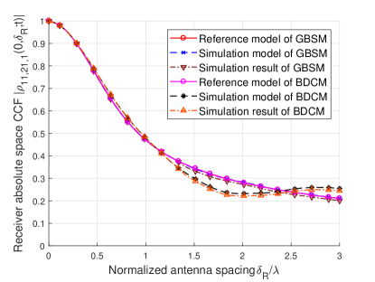
Figure 3: Absolute receiver space CCF $|\rho_{11,21,1}(0,\delta_{R};t)|$ of both models ($M_{R}$ = 32, $M_{T}$ = 32, t = 1 s, $a_{1}$ = 100 m, f = 80 m, $D_{c}^{a}$ = 30 m, $D_{c}^{s}$ = 50 m, $\beta_{R}$ = $\beta_{T}$ = $\pi/2$, $\lambda$ = 0.12 m, $f_{\text{max}}$ = 33.33 Hz, $\alpha_{v}$ = $\pi/6$, $\kappa$ = 5, $\bar{\alpha}_{n}^{R}=\pi/3$, NLOS).

The time correlation properties of both models are illustrated in Fig. 4. It is shown that the time ACFs of the two models are different with the time instant $t$ and the simulation represents the time non-stationarity of both models. Furthermore, the absolute value of time ACF for BDCM is very close to the GBSM. It shows that the time correlation property of the novel BDCM is almost same as the GBSM and there is no loss in time correlation property with the transformation from the antenna to beam domain.

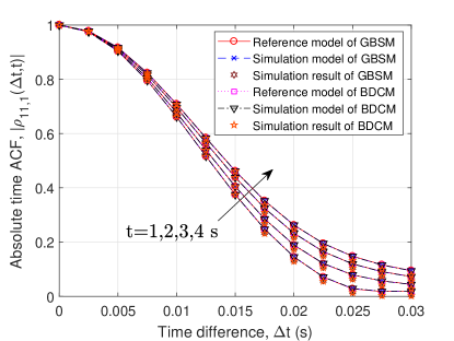
Figure 4: Absolute time ACF of $\text{Cluster}_{1}\left|\rho_{11,1}(\Delta t;t)\right|$ for both models in comparison among t = 1 s, t = 2 s, t = 3 s and t = 4 s ($M_{R}$= 32, $M_{T}$= 32, $a_{1}$=100 m, f=80 m, $D_{c}^{a}$=15 m, $D_{c}^{s}$=50 m, $\beta_{R}=\beta_{T}=\pi/2,\lambda$= 0.15 m, $\delta_{R}=\delta_{T}=0.5\lambda,f_{\max}$=33.33 Hz, $v_{c}$=0.5 m/s, $\mathrm{NLOS},\lambda_{G}$=80 /m, $\lambda_{R}$=4 /m, $P_{F}$=0.3, $\kappa=5$).

Fig. 5 compares the FCFs of BDCM and the existing GBSM under different scenarios. It is shown that the FCFs of two models are exactly the same. Furthermore, the coherence bandwidth of BDCM and the reference ellipse model is almost the same under NLOS condition, which shows that both models have similar frequency correlation properties.

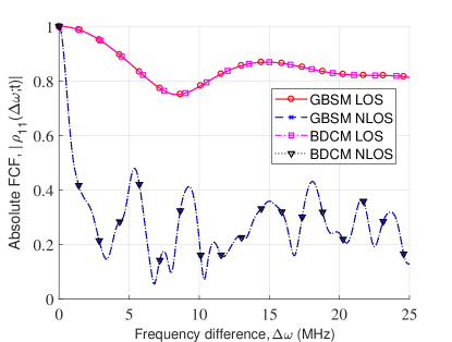
Figure 5: Absolute FCF $|\rho_{11}(\Delta\omega;t)|$ comparison for both models between NLOS and LOS ($M_{R}=32,M_{T}=32,a_{1}$ = 100 m, f = 80 m, $D_{c}^{a}$ = 15 m, $D_{c}^{s}$ = 50 m, $\beta_{R}=\beta_{T}=\pi/2,\lambda$ = 0.15 m, $\delta_{R}=\delta_{T}$ = 0.5$\lambda,f_{\text{max}}$ = 33.33 Hz, $v_{c}$ = 0.5 m/s, $\lambda_{G}$ = 80 /m, $\lambda_{R}$ = 4 /m, $\eta_{c}$ = 0.3, $\kappa=5$).

The complexity comparison of the existing GBSM and the proposed novel BDCM with different antenna pair numbers ($M_{R}\times M_{T}$) is shown in Fig. 6. The complexity increases linearly with the antenna pair number for the GBSM but nonlinear for the BDCM. The number of virtual angles utilized in the BDCM influences the computational complexity and the smaller the number is, the lower computational complexity the model have. It can be observed that when the number of virtual angles is equal to 1, 10 and 20 times of the total number of clusters, the computational complexity of the novel BDCM is much lower than that of GBSM. Thus, The novel BDCM is simpler than the existing GBSM, which will be more conducive to the analysis and research of signal processing and information theory.

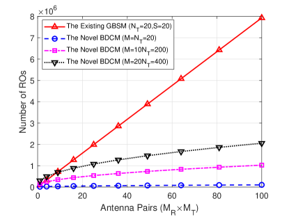
Figure 6: Comparison of the computational complexity for both models ($M_{R}=M_{T}\in\{1,2,\cdots,10\}$, $S=20$, $N_{T}=20$, $M\in\{N_{T},10N_{T},20N_{T}\}$).

VI Conclusions

A novel massive MIMO BDCM with the near-field effect and space-time non-stationarity is proposed. Through the simulation results, we can find that the novel BDCM has the same cluster-level performance as the existing GBSM, and significantly reduces the computational complexity, which is more suitable for the research of signal processing and information theory. In the future work, we will further improve the novel BDCM to make it more general and applicable to various realistic scenarios, and compare it with some latest channel models and measurement data to verify the accuracy of the model, which will be helpful to information theory and signal processing researchers.

References

• [1] X. Ge, K. Huang, C.-X. Wang, X. Hong, and X. Yang, β€œCapacity analysis of a multi-cell multi-antenna cooperative cellular network with co-channel interference,” IEEE Trans. Wireless Commun., vol. 10, no. 10, pp. 3298-3309, Oct. 2011.
• [2] K. Zheng, S. Ou, and X. Yin, β€œMassive MIMO channel models: a survey,” Int. J. Antennas Propag., vol. 2014, pp. 1–8, 2014.
• [3] T. L. Marzetta, β€œMulti-cellular wireless with base stations employing unlimited numbers of antennas,” in Proc. UCSD Information Theory and Applications Workshop, Feb. 2010.
• [4] E. G. Larsson, O. Edfors, F. Tufvesson, and T. L. Marzetta, β€œMassive MIMO for next generation wireless systems,” IEEE Commun. Mag., vol. 52, no. 2, pp. 186–195, Feb. 2014.
• [5] X. Ge, B. Yang, J. Ye, G. Mao, C.-X. Wang and T. Han, β€œSpatial spectrum and energy efficiency of random cellular networks,” IEEE Trans. Commun., vol. 63, no. 3, pp. 1019-1030, Mar. 2015.
• [6] C. X. Wang, J. Bian, and J. Sun, β€œA Survey of 5G Channel Measurements and Models,” IEEE Commun. Surv. Tut., vol. 20, no. 4, pp. 3142-3168, 4th Quarter, 2018.
• [7] S. Wu, C.-X. Wang, H. Haas, el-H. M. Aggoune, M. M. Alwakeel, and B. Ai, β€œA non-stationary wideband channel model for massive MIMO communication systems,” IEEE Trans. Wireless Commun., vol. 14, no. 3, pp. 1434–1446, Mar. 2015.
• [8] S. Wu, C.-X. Wang, el-H. M. Aggoune, M. M. Alwakeel, and Y. He, β€œA non-stationary 3-D wideband twin-cluster model for 5G massive MIMO channels,” IEEE J. Sel. Areas Commun., vol. 32, no. 6, pp. 1207–1218, June 2014.
• [9] S. Wu, C.-X. Wang , el-H. M. Aggoune, M. M. Alwakeel, and X. You,β€œA general 3-D non-stationary 5G wireless channel model,” IEEE Trans. Commun., vol. 66, no. 7, pp. 3065–3078, July 2018.
• [10] C.-X. Wang, S. Wu, L. Bai, X. You, J. Wang, and C. L. I, β€œRecent advances and future challenges for massive MIMO channel measurements and models,” Sci. China Inf. Sci., vol. 59, no. 2, pp. 1–16, Feb. 2016.
• [11] J. P. Kermoal, L. Schumacher, K. I. Pedersen, P. E. Mogensen, and F. Frederiksen, β€œA stochastic MIMO radio channel model with experimental validation,” IEEE J. Sel. Areas Commun., vol. 20, no. 6, pp. 1211–1226, Aug. 2002.
• [12] W. Weichselberger, M. Herdin, H. Γ–zcelik, and E. Bonek, β€œA stochastic MIMO channel model with joint correlation of both link ends,” IEEE Trans. Wireless Commun., vol. 5, no. 1, pp. 90–100, Jan. 2006.
• [13] A. M. Sayeed, β€œDeconstructing multiantenna fading channels,” IEEE Trans. Signal Process., vol. 50, no. 10, pp. 2563–2579, Oct. 2002.
• [14] C. Sun, X. Gao, S. Jin, M. Matthaiou, Z. Ding, and C. Xiao, β€œBeam division multiple access transmission for massive MIMO communications,” IEEE Trans. Commun., vol. 63, no. 6, pp. 2170–2184, June 2015.
• [15] Y. Zhang, A. Ghazal, C.-X. Wang, H. Zhou, W. Duan, and H. Aggoune, β€œAccuracy-complexity tradeoff analysis and complexity reduction methods for non-stationary IMT-A MIMO channel models,” IEEE Access, vol. 7, no. 1, pp. 178047-178062, Dec. 2019.