AdvectiveNet: An Eulerian-Lagrangian
Fluidic reservoir for Point Cloud Processing

Abstract

This paper presents a novel physics-inspired deep learning approach for point cloud processing motivated by the natural flow phenomena in fluid mechanics. Our learning architecture jointly defines data in an Eulerian world space, using a static background grid, and a Lagrangian material space, using moving particles. By introducing this Eulerian-Lagrangian representation, we are able to naturally evolve and accumulate particle features using flow velocities generated from a generalized, high-dimensional force field. We demonstrate the efficacy of this system by solving various point cloud classification and segmentation problems with state-of-the-art performance. The entire geometric reservoir and data flow mimics the pipeline of the classic PIC/FLIP scheme in modeling natural flow, bridging the disciplines of geometric machine learning and physical simulation.

1 Introduction

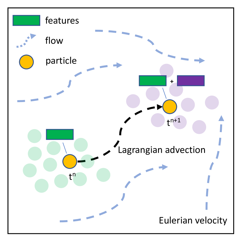
Figure 1: We build an advective network to create a fluidic reservoir with hybrid Eulerian-Lagrangian representations for point cloud processing.

The fundamental mechanism of deep learning is to uncover complex feature structures from large data sets using a hierarchical model composed of simple layers. These data structures, such as a uniform grid (Lecun et al., 1998), an unstructured graph (Kipf & Welling, 2016), or a hierarchical point set (Qi et al., 2016a; 2017), function as geometric reservoirs to yield intricate underpinning patterns by evolving the massive input data in a high-dimensional parameter space. On another front, computational physics researchers have been mastering the art of inventing geometric data structures and simulation algorithms to model complex physical systems (Gibou et al., 2019). Lagrangian structures, which track the motion in a moving local frame such as a particle system (Monaghan, 1992), and Eulerian structures, which describe the evolution in a fixed world frame such as a Cartersian grid (Fedkiw et al., 2001), are the two mainstream approaches. Various differential operators have been devised on top of these data structures to model complex fluid or solid systems.

Pioneered by E (2017) and popularized by many others, e.g., (Long et al., 2018; Chen et al., 2018; Ruthotto & Haber, 2018), treating the data flow as the evolution of a dynamic system is connecting machine learning and physics simulation. As E (2017) notes, there exists a mathematical equivalence between the forward data propagation on a neural network and the temporal evolution of a dynamic system. Accordingly, the training process of a neural network amounts to finding the optimal control forces exerted on a dynamic system to minimize a specific energy form.

Point cloud processing is of particular interest under this perspective. The two main challenges: to build effective convolution stencils and to evolve learned nonlinear features (Qi et al., 2016a; Atzmon et al., 2018; Wang et al., 2019), can map conceptually to the challenges of devising world-frame differential operators and tracking material-space continuum deformations when simulating a PDE-driven dynamic system in computational physics. We envision that the key to solving these challenges lies in the adaption of the most suited geometric data structures to synergistically handle the Eulerian and Lagrangian aspects of the problem. In particular, it is essential to devise data structures and computational paradigms that can accommodate global fast convolutions, and at the same time track the non-linear feature evolution.

The key motivation of this work originates from physical computing that tackles its various frame-dependent and temporally-evolved computational challenges by creating the most natural and effective geometric toolsets under the two different viewpoints. We are specifically interested in uncovering the intrinsic connections between a point cloud learning problem and a computational fluid dynamic (CFD) problem. We observe that the two problems share an important common thread regarding their computational model, which both evolve Lagrangian particles in an Eulerian space guided by the first principle of energy minimization. Such observations shed new insight into the 3D point cloud processing and further opens the door for marrying the state-of-the-art CFD techniques to tackle the challenges emerging in point cloud learning.

To this end, this paper conducts a preliminary exploration to establish an Eulerian-Lagrangian fluidic reservoir that accommodates the learning process of point clouds. The key idea of the proposed method is to solve the point cloud learning problem as a flow advection problem jointly defined in a Eulerian world space and a Lagrangian material space. The defining characteristic distinguishing our method from others is that the spatial interactions among the Lagrangian particles can evolve temporally via advection in a learned flow field, like their fluidic counterpart in a physical circumstance. This inherently takes advantage of the fundamental flow phenomena in evolving and separating Lagrangian features non-linearly (see Figure 1). In particular, we draw the idea of Lagrangian advection on an Eulerian reservoir from both the Particle-In-Cell (PIC) method (Evans & Harlow, 1957) and the Fluid-Implicit-Particle (FLIP) method (Brackbill et al., 1987), which are wholly recognized as ’PIC/FLIP’ in modeling large-scale flow phenomena in both computational fluids, solids, and even visual effects. We demonstrate the result of this synergy by building a physics-inspired learning pipeline with straightforward implementation and matching the state-of-the-art with this framework.

The key contributions of our work include:

• An advective scheme to mimic the natural flow convection process for feature separation;

• A fluid-inspired learning paradigm with effective particle-grid transfer schemes;

• A fully Eulerian-Lagrangian approach to process point clouds, with the inherent advantages in creating Eulerian differential stencils and tracking Lagrangian evolution;

• A simple and efficient physical reservoir learning algorithm.

2 Related Works

This section briefly reviews the recent related work on point cloud processing. According to data structures used for building the convolution stencil, the methods can be categorized as Lagrangian (using particles only), Eulerian (using a background grid), and hybrid (using both). We also review the physical reservoir methods that embed network training into a physical simulation process.

Lagrangian

Lagrangian methods build convolution operators on the basis of local points. Examples include PointNet (Qi et al., 2016a), which conducts max pooling to combat any disorganized points, PointNet++ (Qi et al., 2017), which leverages farthest point sampling to group particles, and a set of work (Wang et al., 2019; Xu et al., 2018; Li et al., 2018b; a; Jiang et al., 2018) based on k-nearest neighbors. Beyond the mesh-free approaches, researchers also seek to build effective point-based stencils by establishing local connectivities among points. Most significantly, geometric deep learning (Bruna et al., 2013; Bronstein et al., 2016) builds convolution operators on top of a mesh to uncover the intrinsic features of objects’ geometry. In particular, we want to highlight the work on dynamic graph CNN (Wang et al., 2019), which builds directed graphs in an extemporaneous fashion in feature space to guide the point neighbor search process, which shares similarities with our approach.

Eulerian

Eulerian approaches leverage background discretizations to perform computation. The most successful Eulerian method is the CNN (Lecun et al., 1998), which builds the convolution operator on a 2D uniform grid. This Eulerian representation can be used to process 3D data by using multiple views (Su et al., 2015; Qi et al., 2016b; Feng et al., 2018) and extended to 3D volumetric grids (Maturana & Scherer, 2015; Qi et al., 2016b; Z. Wu, 2015). Grid resolution is the main performance bottleneck for 3D CNN methods. Adaptive data structures such as Octree (Riegler et al., 2016; Wang et al., 2017; 2018), Kd-tree (Klokov & Lempitsky, 2017), and multi-level 3D CNN (Ghadai et al., 2018) were invented to alleviate the problem. Another example of Eulerian structures is Spherical CNN (Cohen et al., 2018) that projects 3D shapes onto a spherical coordinate system to define equivalent rotation convolution. In addition to these voxel-based, diffusive representations, shapes can also be described as a sharp interface modeled as an implicit level set function (Hu et al., 2017; Park et al., 2019; Mescheder et al., 2019). For each point in the space, the level set function acts as a binary classifier checking whether the point is inside the shape or not.

Hybrid

There have been recent attempts to transfer data between Lagrangian and Eulerian representations for efficient convolution implementation. These data transfer methods can be one-way (Wang et al., 2017; Klokov & Lempitsky, 2017; Tchapmi et al., 2017; Le & Duan, 2018), in which case the data is mapped from points to grid cells permanently, or two-way (Su et al., 2018; Atzmon et al., 2018; Liu et al., 2019; Groueix et al., 2018), in which case data is pushed forward from particle to grid for convolution and pushed backward from grid to particle for evolution. Auto-encoders on point clouds (Fan et al., 2016; Achlioptas et al., 2017; Yang et al., 2017; Yu et al., 2018; Zhao et al., 2019) can be also regarded as a hybrid approach, where encoded data is Eulerian and decoded data is Lagrangian. In addition, we want to mention the physical reservoir computing techniques that focus on the leverage of the temporal, physical evolution to solve learning problems, e.g., see (Jaeger, 2001) and (Maass et al., 2002). Physical reservoir computing is demonstrating successes in various applications (Jalalvand et al., 2015; Jaeger, 2002; Hauser et al., 2012; Lukoševičius & Jaeger, 2009; Tanaka et al., 2019).

3 Algorithm

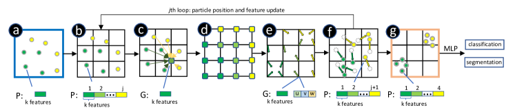
Figure 2: Workflow overview: a) The feature vector for each particle is initialized by a $1\times 1$ convolution; b) Particles are embedded in an Eulerian grid; c) Features are interpolated from particles to the grid, denoted as ${\bm{I}}_{P}^{G}$; d) 3D convolution is applied on the grid to calculate the generalized forces and grid features; e) A velocity field is generated on the background grid; f) Particles advect in the Eulerian space using the interpolated velocities; grid features are interpolated to particles, denoted as ${\bm{I}}_{G}^{P}$, and appended to its feature vector; g) Particles aggregate. The workflow consists of one loop to update the particle positions and features iteratively with temporal evolution. Finally, the Lagrangian features are fed into a fully-connected network for classification and segmentation.

PIC/FLIP overview

Before describing the details of our method, we begin with briefly surveying the background of the PIC/FLIP method. PIC/FLIP uses a hybrid grid-particle representation to describe fluid evolution. The particles are used for tracking materials, and the grid is used for discretizing space. Properties such as mass, density, and velocity are carried on particles. Each simulation step consists of four substeps: particle-to-grid transfer ${\bm{I}}_{P}^{G}$, grid force calculation (Projection), grid-to-particle transfer ${\bm{I}}_{G}^{P}$, and moving particles (Advection). In the ${\bm{I}}_{P}^{G}$ step, the properties on each particle are interpolated onto a background grid. In the Projection step, calculations such as adding body forces and enforcing incompressibility are conducted on the background grid. After this, the velocities on grid nodes are interpolated back onto particles, i.e., ${\bm{I}}_{G}^{P}$. Finally, particles move to their new positions for the next time step using the updated velocities (Advection). As summarized above, the key philosophy of PIC/FLIP is to carry all features on particles and to perform all differential calculations on the grid. The background grid functions as a computational paradigm that can be established extemporaneously when needed. Data will transfer from particle to grid and then back to particle to finish a simulation loop.

Our proposed approach follows the same design philosophy as PIC/FLIP by storing the learned features on particles and conducting differential calculations on the grid. The Lagrangian features will evolve with the particles moving in an Eulerian space and interact with local grid nodes. As shown in Figure 2, the learning pipeline mimics the PIC/FLIP simulation loop in the sense that Lagrangian particles are advected passively in an Eulerian space guided by a learned velocity field.

Initialization

We initialize a particle system ${\bm{P}}$ and a background grid ${\bm{G}}$ as the Lagrangian and Eulerian representations respectively for processing point clouds. We use the subscript $p$ to refer to particle indices and $i$ to refer to the grid nodes. For the Lagrangian portion, the particle system has $n$ particles, with each particle $P_{p}$ carrying its position ${\bm{x}}_{p}\in{\mathbb{R}}^{3}$, velocity ${\bm{v}}_{p}\in{\mathbb{R}}^{3}$, mass $m_{p}\in{\mathbb{R}}$, and a feature vector ${\bm{f}}_{p}\in{\mathbb{R}}^{k}$ ($k=64$ initially). The particle velocity is zero at the beginning. The particle mass $m_{p}=1$ will keep constant over the entire evolution. To initialize the feature vector ${\bm{f}}_{p}$, we first put the particles in a grid with size $N^{3}$. For each cell, we calculate 1) the center of mass of all the particles in the cell, and 2) the normalized vector pointing from each particle to the this mass center. For each particle, we concatenate these two vectors to the initial feature vector. This process is repeated for $N=2,4,6,8,10,12$. The resulting feature vector with the length of $6\times 6$ are fed into a multi-layer perceptron (MLP) to generate the feature vector ${\bm{f}}_{p}$.

For the Eulerian part, we start with a 3D uniform grid ${\bm{G}}$ to represent the bounding box of the particles. The resolution of the grid is $N^{3}$ ($N=16$ for most of our cases). At the beginning, the particle system and its bounding box are normalized to the space of $[-1,1]^{3}$. Each grid node $G_{i}$ of ${\bm{G}}$ stores data interpolated from the particles.

Particle-grid transfer

Both the interpolation from grid to particle and particle to grid are executed using tri-linear interpolation, which is a common scheme for property transfer in simulation and learning code.

Generalized grid forces

With the feature vectors transferred from particles to grid nodes, we devise a 3D CNN on the grid to calculate a generalized force field based on the Eulerian features. The network consists of three convolution layers, with each layer as a combination of 3D convolution, batch norm, and ReLU. The input of the network is a vector field ${\bm{\mathsfit{F}}}^{(kj)\times N\times N\times N}$ composed of the feature vectors on all grid nodes, with $k$ as the feature vector size ($64$ by default) and $j$ as the iteration index in the evolution loop (see Figure 2). The output is a convoluted vector field ${\bm{\mathsfit{F}}}_{c}^{(kj)\times N\times N\times N}$ with the same size as ${\bm{\mathsfit{F}}}$.

We use ${\bm{\mathsfit{F}}}_{c}$ for two purposes: 1) To interpolate ${\bm{\mathsfit{F}}}_{c}$ from the grid back onto particles and append it to the current feature vector in order to enrich its feature description; 2) To feed ${\bm{\mathsfit{F}}}_{c}$ into another single-layer network to generate the new Eulerian velocity field ${\bm{\mathsfit{V}}}$ for the particle advection. Specifically, this ${\bm{\mathsfit{V}}}$ is interpolated back onto particles in the same way as the feature interpolation to update the particle positions for the next iteration (see Advection for details).

Advection

The essence of an advection process is to solve the advection equation with the Lagrangian form $D{\bm{v}}/Dt=0$ or the Eulerian form $\partial{\bm{v}}/\partial t+{\bm{v}}\cdot\nabla{\bm{v}}=0.$ The advection equation describes the passive evolution of particle properties within a flow field. With the learned grid velocity field in hand, we will update the particle velocity following the conventional scheme of PIC/FLIP. Specifically, the new velocity is first updated by interpolating the Eulerian velocity to particles (the PIC step):

$${\bm{v}}^{n+1}_{PIC}={\bm{I}}_{G}^{P}({\bm{v}}^{n+1}_{g})$$ (1)

Then, we interpolate the difference between the new and the old Eulerian velocity:

$${\bm{v}}^{n+1}_{FLIP}={\bm{v}}^{n}_{p}+{\bm{I}}_{G}^{P}({\bm{v}}^{n+1}_{g}-{\bm{I}}_{P}^{G}({\bm{v}}^{n}_{p})),$$ (2)

and then add them to the particle with a weight $\alpha$ (=0.5 in default.):

$${\bm{v}}^{n+1}_{p}=\alpha*{\bm{v}}^{n+1}_{PIC}+(1-\alpha)*{\bm{v}}^{n+1}_{FLIP}$$ (3)

With the updated velocity on each particle from the ${\bm{I}}_{G}^{P}$ interpolation, the particle’s position for the next time step can be updated using a standard time integration scheme (explicit Euler in our implementation):

$${\bm{x}}^{n+1}_{p}={\bm{x}}^{n}_{p}+{\bm{v}}^{n+1}_{p}\Delta t.$$ (4)

Boundary conditions

We apply a soft boundary constraints by adding an penalty term in the objective function to avoid particles moving outside of the grid:

$$\phi_{b}=\frac{1}{n}\sum_{p}max(0,\|x_{p}\|_{2}-1)$$ (5)

where $x_{p}$ represents the $p$th particle in the whole batch and $n$ is the number of particles in the whole batch. We penalize on all the particles that run outside the grid.

We also design the gather penalty and the diffusion objectives to enhance the particle diffusion and clustering effects during evolution (specifically for the segmentation application):

$$\phi_{g} =\frac{1}{2}\sum_{l}\sum_{m}max(0,1-\|c_{l}-c_{m}\|)$$ (6)

$$\phi_{d} =\frac{1}{n}\sum_{l}\sum_{p}\|c_{l}-x_{lp}\|$$ (7)

where $c_{l}$ and $c_{m}$ are the centers of particles of label $l$ and $m$ and $x_{lp}$ is the $p$th particle with label $l$.

4 Network Architecture

The global architecture of our network is shown in Figure 3. Our model starts from a point cloud with the position of each point. After an initialization step ending with a two-layer MLP (64,64), each point carries a feature vector of length 64. These features are fed into the advection module to exchange information with neighbors. The generated features have two uses: to generate the velocity for each particle, and to be used along with the new advected particle position to collect information from neighbors. This process repeats for a few times to accumulate features in the feature space and to aggregate particles in the physical space.

Advection module

The data flow inside the advection module starts with particles, passes through layers of grids, then sinks back to particles. This module takes the position and the feature vector as input. The feature vectors are first fed into an MLP to reduce its dimensions to 32, which saves computational time and prevents over-fitting. Then, we apply three layers of convolution that are each a combination of 3D convolution, batch norm, and ReLU, with a hidden-layer size as (32,16,32) on the grid, to obtain a high-dimensional, generalized force field on the grid. Afterwards, a velocity field is generated from this force field by another two-layer network. The velocity field is then interpolated back to particles for Lagrangian advection. Additionally, to generate the output feature vector, the input and output features (with 32-dimension each) are concatenated together and appended to the original feature vector. The output of the advection module is a set of particles with new positions and new features that are ready to process for the next iteration as in Figure 2.

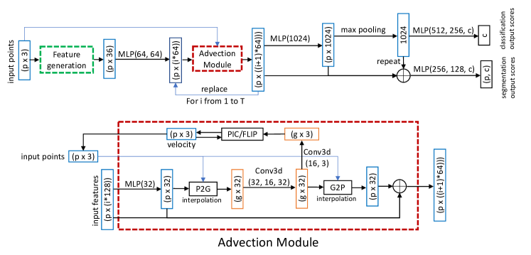
Figure 3: Network architectures: The top diagram demonstrates the global architecture of our network with detailed information for tensor dimensionality and modular connectivity. The blue box is for particle states and the orange box indicates grid states. The dotted green box is the module generating the initial Lagrangian features. The dotted red box is for the functional module of advection (see the bottom diagram). The states are connected with multi-layer perceptrons (black arrows in the diagram). Each MLP has a number of hidden layers with a different number of neurons (specified by the numbers within the parentheses). The bottom figure shows the details of the advection module updating the particle features by transferring data on the grid and concatenating particles. Meanwhile, it updates the particle positions with the generalized Eulerian forces calculated on the grid.

5 Experiments

We conducted three parts of experiments, including the ablation tests and the applications for classification and segmentation. We implemented the system in PyTorch (see the submitted source code) and conducted all the tests on a single RTX 2080 Ti GPU. In the ablation tests, we evaluated the functions of the advection module, temporal resolution, grid resolution, and the functions of the PIC/FLIP scheme on ModelNet10 (Z. Wu, 2015) and ShapeNet (Yi et al., 2016). For classification, we tested our network on ModelNet40 and its subset ModelNet10. We used the class prediction accuracy as our metric. For segmentation, we tested our network on ShapeNet (Yi et al., 2016) and S3DIS data set (Armeni et al., 2016). We used mean Intersection over Union (mIoU) to evaluate our method and compare with other benchmarks.

5.1 Ablation Experiments

Advection

We turn off the advection module to verify the its effectiveness for the final performance. We conducted the comparison on the ShapeNet data set (Yi et al., 2016). The mIoU reached $86.2\%$ with the advection module in comparison to $85.3\%$ without it, necessitating the role of the advection step.

Temporal resolution

Table 1: Temporal resolution

# ts	0	1	2	3	4	5	6	7	8
Acc	93.2	95.2	95.4	94.8	94.7	95.1	95.1	95.2	95.1

(Physical Intuition) The evolution of a dynamic system can be discretized on the temporal axis by the numerical integration with a number of steps. Given a fixed total time, the number of timesteps is in an inverse ratio to the length of each step. For a typical explicit scheme (e.g., explicit Euler), a small timestep leads to a numerically secure result at the expense of performing more time integrations; while a large timestep, although efficient, might explode out of the stable region.

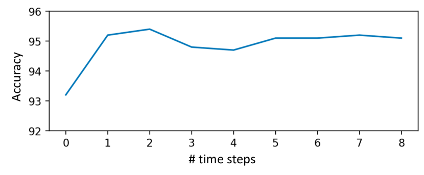
Figure 4: Temporal accuracy

(Numerical Tests) Motivated by this numerical intuition, we investigated the effects of temporal resolution on our learning problem. Specifically, we tested the performance of the network regarding both the learning accuracy and the evolved shape by subdividing the numerical integration into 0-8 steps (0 means no integration). The test was performed on ModelNet10. As shown in Table 1 and Figure 4, the learning accuracy stabilizes around $95\%$ as the number of integration increases, with 2 steps and 4 steps as the maximum ($95.4\%$) and minimum ($94.7\%$), indicating a minor effect from the temporal resolution on learning accuracy. For the shape convergence, we demonstrated that different temporal resolutions converge to very similar final equilibrium states, despite of the different time step sizes. As shown in Figure 5, the point-cloud model of an airplane is advected with different velocity fields generated on different temporal resolutions. The final shapes with timestep 2, 3, and 6 all exhibit the same geometric feature separations and topological relations. This result evidences our conjecture that all the temporal resolutions we used are within the stable region, motivating us to pick a larger time step size (total time/3 for most of our cases) for efficiency.

Spatial resolution

Table 2: Spatial resolution

	$8^{3}$	$16^{3}$	$32^{3}$
ModelNet10 Acc (1024 pnts)	94.4	95.4	95.1
ModelNet10 pnts per cell	6.8	1.6	1.0
ShapeNet mIoU (2048 pnts)	85.4	86.1	86.2
ShapeNet pnts per cell	21.4	5.2	1.7

(Physical Intuition) For a typical particle-grid simulation in CFD, the resolution of the grid and the number of particles are correlated. Making sure that each grid cell should contain enough number of particles (e.g., 1-2 particles per cell), ensures information exchange between these two discretizations is accurate. Empirically, an overly refined grid will lead to inaccurate Eulerian convolution due to the large bulk of empty cells, while an overly coarse grid will dampen the motion of particles due to artificial viscosity (e.g., see Evans & Harlow (1957); Brackbill et al. (1987)), which makes the number of particles per cell $ppc$ a key hyperparameter.

(Numerical Validation) We validate this grid-particle design art from scientific computing by testing our network with different grid resolutions. As shown in Table 2, we tested the grid resolution of $8^{3}$, $16^{3}$, and $32^{3}$ on two datasets with 1024 and 2048 particles separately. We observed that a $16^{3}$ grid fits the $1024$ dataset best and a $32^{3}$ grid fits the $2048$ dataset best. By calculating the average $ppc$ for each case, we made a preliminary conclusion that the optimal $ppc$ is around 1.5-1.8. This also implies an optimal grid resolution for a point-set with $N$ particles to be $(ppc*N)^{1/3}$.

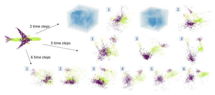
Figure 5: Visualization of the advection of an airplane is shown with time steps of 2, 3 and 6. Note that we rotate the point cloud and normalize the velocity field for visualization purposes.

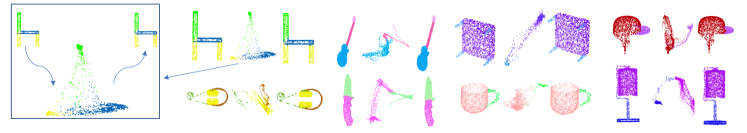
Figure 6: Visualization of segmentation. Examples of different categories are depicted, consisting of initial shape, intermediary grouping, and final part prediction.

PIC/FLIP

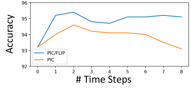
Figure 7: PIC/FLIP VS PIC

(Physical Intuition) Temporal smoothness is key for developing a dynamic system to achieve its equilibrium state. PIC/FLIP obtains such smoothness by averaging weighted velocities between two adjacent time steps. (Numerical Validation) To highlight the role of this averaging, we compared the accuracy between PIC/FLIP and PIC only (no temporal averaging) on ModelNet10. We can see from Figure 7 that the model with PIC/FLIP quickly stabilizes to a high accuracy, outperforming the model with PIC only.

5.2 Applications

Classification

Table 3: Classification on ModelNet.

Method	Input	ModelNet10	ModelNet40
SO-Net	2048 pnts	94.1	90.9
PCNN	1024 pnts	94.9	92.3
PointNet	1024 pnts	-	89.2
PointGrid	1024 pnts	-	92.0
DGCNN	1024 pnts	-	92.9
PointCNN	1024 pnts	-	92.5
PointNet++	pnts, nors	-	91.9
SpiderCNN	pnts, nors	-	92.4
O-CNN	octree, nors	91.0	86.5
VoxNet	grid ($32^{3}$)	92.0	83.0
Kd-Net	kd-tree	94.0	91.8
FPNN	grid	-	87.5
MRCNN	multi-level vox	91.3	86.2
Ours ($16^{3}$)	1024 pnts	95.4	92.8

We tested our network on ModelNet40 (Z. Wu, 2015) and ModelNet10 for classification. We use a grid resolution $16^{3}$ to train both the networks. As shown in Table 3, our result outperforms the state-of-art on ModelNet10, noticeably surpassing those using grids. On ModelNet40, our result rivals DGCNN (92.8% v.s. 92.9%). But our parameter number is significantly smaller than DGCNN ($1M$ v.s. $21M$.)

Segmentation

We tested our algorithm for object part segmentation on ShapeNet (Yi et al., 2016). We used a grid resolution and $32^{3}$ for training and testing. We showed the state-of-art performance of our approach in Table 4. Since the category of each input object is known beforehand, we trained separate models for each category. Note that we only compared with point-based methods that had similar input (points or/and normals) as ours. It can be seen that we outperform all the state-of-art with less parameters ($1.1M$, 2 time steps) Some examples animating the segmentation process can be seen in Figure 6.

Table 4: Segmentation results on ShapeNet.

Method	input	mIoU	aero	bag	cap	car	chair	ear phone	guitar	knife	lamp	laptop	motor	mug	pistol	rocket	skate board	table
PointNet	2k pnts	83.7	83.4	78.7	82.5	74.9	89.6	73.0	91.5	85.9	80.8	95.3	65.2	93.0	81.2	57.9	72.8	80.6
PCNN	2k pnts	85.1	82.4	80.1	85.5	79.5	90.8	73.2	91.3	86.0	85.0	95.7	73.2	94.8	83.3	51.0	75.0	81.8
Kd-Net	4k pnts	82.3	80.1	74.6	74.3	70.3	88.6	73.5	90.2	87.2	81.0	94.9	57.4	86.7	78.1	51.8	69.9	80.3
DGCNN	2k pnts	85.1	84.2	83.7	84.4	77.1	90.9	78.5	91.5	87.3	82.9	96.0	67.0	93.3	82.6	59.7	75.5	82.0
PointCNN	2k pnts	86.1	84.1	86.4	86.0	80.8	90.6	79.7	92.3	88.4	85.3	96.1	77.2	95.2	84.2	64.2	80.0	82.9
PointNet++	pnts, nors	85.1	82.4	79.0	87.7	77.3	90.8	71.8	91.0	85.9	83.7	95.3	71.6	94.1	81.3	58.7	76.4	82.6
SO-Net	pnts, nors	84.9	82.8	77.8	88.0	77.3	90.6	73.5	90.7	83.9	82.8	94.8	69.1	94.2	80.9	53.1	72.9	83.0
SpiderCNN	pnts, nors	85.3	83.5	81.0	87.2	77.5	90.7	76.8	91.1	87.3	83.3	95.8	70.2	93.5	82.7	59.7	75.8	82.8
SPLATNet	pnts, img	85.4	83.2	84.3	89.1	80.3	90.7	75.5	92.1	87.1	83.9	96.3	75.6	95.8	83.8	64.0	75.5	81.8
Ours ($32^{3}$)	2k pnts	86.2	84.4	83.8	85.7	81.7	91.1	74.7	91.7	87.2	84.9	96.4	72.2	95.9	84.3	58.5	75.1	83.4

6 Discussion and Conclusion

This paper presents a new perspective in treating the point cloud learning problem as a dynamic advection problem using a learned background velocity field. The key technical contribution of the proposed approach is to jointly define the point cloud learning problem as a flow advection problem in a world space using a static background grid and the local space using moving particles. Compared with the previous hybrid grid-point learning methods, e.g. two-way coupled particle-grid schemes (Su et al., 2018; Atzmon et al., 2018; Liu et al., 2019), our approach solves the learning problem from a dynamic system perspective which accumulates features in a flow field learned temporally. The coupled Eulerian-Lagrangian data structure in conjunction with its accommodated interpolation schemes provide an effective solution to tackle the challenges regarding both stencil construction and feature evolution by leveraging a numerical infrastructure that is matured in the scientific computing community. On another hand, our approach can be thought of as an exploration in creating a new physical reservoir motivated by continuum mechanics in order to find alternative solutions for the conventional point cloud processing networks. Thanks to the low-dimensional physical space and the large time step our network allows, our learning accuracy rivals the state-of-the-art deep networks such as PointCNN (Li et al., 2018b) and DGCNN (Wang et al., 2019) while using significantly fewer network parameters ($4\%$ to $25\%$ in our comparisons). Our future plan is to scale the algorithm to larger data sets and handle more complex point clouds with sparse and adaptive grid structures.

7 Acknowledgement

This project is support in part by Dartmouth Neukom Institute CompX Faculty Grant, Burke Research Initiation Award, and NSF MRI 1919647. Helen Lu Cao is supported by the Dartmouth Women in Science Project (WISP) and Undergraduate Advising and Research Program (UGAR).

Appendix A Performance on S3DIS

In this part, we further discuss our algorithm and its performance on the large-scale S3DIS dataset (Armeni et al., 2017). Unlike ModelNet and ShapeNet, the S3DIS consists of colored point clouds collected from real world. We train on the area 1,2,3,4,6 and test on the area 5. We make some modifications on our network structure to better fir this dataset.

1. We set the number of time steps to 4 instead of 2.

2. To allow large number of time steps (deeper networks), we replace our original MLP with the ResNet blocks (He et al., 2015).

3. We use two more MLPs to encode the initial features on each point.

4. We scale the point cloud into the space $[-0.9,0.9]^{3}$ because the data contains many points on the border plane, such as ceiling and floor.

The performance on the S3DIS is in the table 5.

Table 5: Segmentation results on S3DIS.

Method	mIoU	ceiling	floor	wall	beam	column	window	door	table	chair	sofa	bookcase	board	clutter
PointNet	41.09	88.80	97.33	69.80	0.05	3.92	46.26	10.76	58.93	52.61	5.85	40.28	26.38	33.22
SPGraph	58.04	89.35	96.87	78.12	0.00	42.81	48.93	61.58	84.66	75.41	69.84	52.60	2.10	52.22
SegCloud	48.92	90.06	96.05	69.86	0.00	18.37	38.35	23.12	70.40	75.89	40.88	58.42	12.96	41.60
PCCN	58.27	92.26	96.20	75.89	0.27	5.98	69.49	63.45	66.87	65.63	47.28	68.91	59.10	46.22
PointCNN	57.26	92.31	98.24	79.41	0.00	17.60	22.77	62.09	74.39	80.59	31.67	66.67	62.05	56.74
Ours	54.37	92.41	98.28	74.88	0.68	18.74	45.36	48.70	74.11	78.50	35.60	57.02	38.84	43.73

From the table we can see that the result obtained by AdvectiveNet is comparable to the states of the art (with the highest mIoU in ceiling, floor, and beam), though it is less impressive to the performance on ModelNet and ShapeNet. We observe that, in the S3DIS, the relative positions of different parts are more flexible and less structured compared to ModelNet and ShapeNet. For example, in ShapeNet, the wings of the airplanes are always on the two sides of the fuselages. Hence, we would interpret our performance on ShapeNet thanks to the ability in detecting intrinsic structures underlying the relative positions of the parts. The tendency to focus on relative positions also explains why our algorithm outperforms the states of the art on detecting ceiling and floor (they are always on the two sides of the rooms).

Appendix B Implementation Details

We follow the data augmentation methods in (Li et al., 2018b). We use dropout ratio 0.3 on the last fully connected layer before class score prediction. The decay rate for batch normalization starts with 0.5 and is gradually decreased to 0.01. We use adamw optimizer (Loshchilov & Hutter, 2017) with initial learning rate 0.001, weight decay rate 0.005, momentum 0.9 and batch size 32. The learning rate is multiplied by 0.8 every 20 epochs. We train the model for 200 epochs. We use the label smoothing techique (Pereyra et al., 2017) with confidence 0.8. We use the grid size 16 and 32 for classification and segmentation, respectively.

References

- Achlioptas et al. (2017) Panos Achlioptas, Olga Diamanti, Ioannis Mitliagkas, and Leonidas J. Guibas. Representation learning and adversarial generation of 3d point clouds. CoRR, abs/1707.02392, 2017.
- Armeni et al. (2017) I. Armeni, A. Sax, A. R. Zamir, and S. Savarese. Joint 2D-3D-Semantic Data for Indoor Scene Understanding. ArXiv e-prints, February 2017.
- Armeni et al. (2016) Iro Armeni, Ozan Sener, Amir R. Zamir, Helen Jiang, Ioannis Brilakis, Martin Fischer, and Silvio Savarese. 3d semantic parsing of large-scale indoor spaces. In The IEEE Conference on Computer Vision and Pattern Recognition (CVPR), June 2016.
- Atzmon et al. (2018) Matan Atzmon, Haggai Maron, and Yaron Lipman. Point convolutional neural networks by extension operators. CoRR, abs/1803.10091, 2018.
- Brackbill et al. (1987) J. U. Brackbill, D. B. Kothe, and H. M. Ruppel (eds.). FLIP (Fluid-Implicit-Particle): A low-dissipation, particle-in-cell method for fluid flow, April 1987.
- Bronstein et al. (2016) Michael M. Bronstein, Joan Bruna, Yann LeCun, Arthur Szlam, and Pierre Vandergheynst. Geometric deep learning: going beyond euclidean data. CoRR, abs/1611.08097, 2016.
- Bruna et al. (2013) Joan Bruna, Wojciech Zaremba, Arthur Szlam, and Yann LeCun. Spectral networks and locally connected networks on graphs. CoRR, abs/1312.6203, 2013.
- Chen et al. (2018) Ricky T. Q. Chen, Yulia Rubanova, Jesse Bettencourt, and David Duvenaud. Neural ordinary differential equations. Advances in Neural Information Processing Systems, 2018.
- Cohen et al. (2018) Taco S. Cohen, Mario Geiger, Jonas Köhler, and Max Welling. Spherical cnns. CoRR, abs/1801.10130, 2018.
- E (2017) Weinan E. A proposal on machine learning via dynamical systems. Communications in Mathematics and Statistics, 5(1):1–11, Mar 2017. ISSN 2194-671X. doi: 10.1007/s40304-017-0103-z.
- Evans & Harlow (1957) M.W. Evans and F.H. Harlow. The particle-in-cell method for hydrodynamic calculations. 6 1957.
- Fan et al. (2016) Haoqiang Fan, Hao Su, and Leonidas J. Guibas. A point set generation network for 3d object reconstruction from a single image. CoRR, abs/1612.00603, 2016.
- Fedkiw et al. (2001) Ronald Fedkiw, Jos Stam, and Henrik Wann Jensen. Visual simulation of smoke. In Proceedings of the 28th Annual Conference on Computer Graphics and Interactive Techniques, SIGGRAPH ’01, pp. 15–22, New York, NY, USA, 2001. ACM. ISBN 1-58113-374-X. doi: 10.1145/383259.383260.
- Feng et al. (2018) Yifan Feng, Zizhao Zhang, Xibin Zhao, Rongrong Ji, and Yue Gao. Gvcnn: Group-view convolutional neural networks for 3d shape recognition. In The IEEE Conference on Computer Vision and Pattern Recognition (CVPR), June 2018.
- Ghadai et al. (2018) Sambit Ghadai, Xian Yeow Lee, Aditya Balu, Soumik Sarkar, and Adarsh Krishnamurthy. Multi-resolution 3d convolutional neural networks for object recognition. CoRR, abs/1805.12254, 2018. URL http://arxiv.org/abs/1805.12254.
- Gibou et al. (2019) Frederic Gibou, David Hyde, and Ron Fedkiw. Sharp interface approaches and deep learning techniques for multiphase flows. Journal of Computational Physics, 380:442–463, 2019.
- Groueix et al. (2018) Thibault Groueix, Matthew Fisher, Vladimir G. Kim, Bryan Russell, and Mathieu Aubry. AtlasNet: A Papier-Mâché Approach to Learning 3D Surface Generation. In Proceedings IEEE Conf. on Computer Vision and Pattern Recognition (CVPR), 2018.
- Hauser et al. (2012) Helmut Hauser, Auke J. Ijspeert, Rudolf M. Füchslin, Rolf Pfeifer, and Wolfgang Maass. The role of feedback in morphological computation with compliant bodies. Biological Cybernetics, 106(10):595–613, Nov 2012. ISSN 1432-0770. doi: 10.1007/s00422-012-0516-4.
- He et al. (2015) Kaiming He, Xiangyu Zhang, Shaoqing Ren, and Jian Sun. Deep residual learning for image recognition. arXiv preprint arXiv:1512.03385, 2015.
- Hu et al. (2017) Ping Hu, Bing Shuai, Jun Liu, and Gang Wang. Deep level sets for salient object detection. 2017 IEEE Conference on Computer Vision and Pattern Recognition (CVPR), pp. 540–549, 2017.
- Jaeger (2001) Herbert Jaeger. The” echo state” approach to analysing and training recurrent neural networks-with an erratum note’. Bonn, Germany: German National Research Center for Information Technology GMD Technical Report, 148, 01 2001.
- Jaeger (2002) Herbert Jaeger. Adaptive nonlinear system identification with echo state networks. In NIPS, 2002.
- Jalalvand et al. (2015) Azarakhsh Jalalvand, Glenn Wallendael, and Rik Van de Walle. Real-time reservoir computing network-based systems for detection tasks on visual contents. pp. 146–151, 06 2015. doi: 10.1109/CICSyN.2015.35.
- Jiang et al. (2018) Mingyang Jiang, Yiran Wu, and Cewu Lu. Pointsift: A sift-like network module for 3d point cloud semantic segmentation. CoRR, abs/1807.00652, 2018.
- Kipf & Welling (2016) Thomas N. Kipf and Max Welling. Semi-supervised classification with graph convolutional networks. CoRR, abs/1609.02907, 2016.
- Klokov & Lempitsky (2017) Roman Klokov and Victor S. Lempitsky. Escape from cells: Deep kd-networks for the recognition of 3d point cloud models. CoRR, abs/1704.01222, 2017.
- Le & Duan (2018) Truc Le and Ye Duan. Pointgrid: A deep network for 3d shape understanding. In The IEEE Conference on Computer Vision and Pattern Recognition (CVPR), June 2018.
- Lecun et al. (1998) Yann Lecun, Leon Bottou, Y Bengio, and Patrick Haffner. Gradient-based learning applied to document recognition. Proceedings of the IEEE, 86:2278 – 2324, 12 1998. doi: 10.1109/5.726791.
- Li et al. (2018a) Jiaxin Li, Ben M. Chen, and Gim Hee Lee. So-net: Self-organizing network for point cloud analysis. CoRR, abs/1803.04249, 2018a.
- Li et al. (2018b) Yangyan Li, Rui Bu, Mingchao Sun, Wei Wu, Xinhan Di, and Baoquan Chen. Pointcnn: Convolution on x-transformed points. In S. Bengio, H. Wallach, H. Larochelle, K. Grauman, N. Cesa-Bianchi, and R. Garnett (eds.), Advances in Neural Information Processing Systems 31, pp. 820–830. Curran Associates, Inc., 2018b.
- Liu et al. (2019) Zhijian Liu, Haotian Tang, Yujun Lin, and Song Han. Point-voxel CNN for efficient 3d deep learning. CoRR, abs/1907.03739, 2019.
- Long et al. (2018) Zichao Long, Yiping Lu, Xianzhong Ma, and Bin Dong. PDE-net: Learning PDEs from data. In Jennifer Dy and Andreas Krause (eds.), Proceedings of the 35th International Conference on Machine Learning, volume 80 of Proceedings of Machine Learning Research, pp. 3208–3216, Stockholmsmässan, Stockholm Sweden, 10–15 Jul 2018. PMLR.
- Loshchilov & Hutter (2017) Ilya Loshchilov and Frank Hutter. Fixing weight decay regularization in adam. CoRR, abs/1711.05101, 2017. URL http://arxiv.org/abs/1711.05101.
- Lukoševičius & Jaeger (2009) Mantas Lukoševičius and Herbert Jaeger. Reservoir computing approaches to recurrent neural network training. Computer Science Review, 3(3):127 – 149, 2009. ISSN 1574-0137. doi: https://doi.org/10.1016/j.cosrev.2009.03.005.
- Maass et al. (2002) Wolfgang Maass, Thomas Natschläger, and Henry Markram. Real-time computing without stable states: A new framework for neural computation based on perturbations. Neural Comput., 14(11):2531–2560, November 2002. ISSN 0899-7667. doi: 10.1162/089976602760407955.
- Maturana & Scherer (2015) D. Maturana and S. Scherer. VoxNet: A 3D Convolutional Neural Network for Real-Time Object Recognition. In IROS, 2015.
- Mescheder et al. (2019) Lars Mescheder, Michael Oechsle, Michael Niemeyer, Sebastian Nowozin, and Andreas Geiger. Occupancy networks: Learning 3d reconstruction in function space. In Proceedings IEEE Conf. on Computer Vision and Pattern Recognition (CVPR), 2019.
- Monaghan (1992) Joe J Monaghan. Smoothed particle hydrodynamics. Annual review of astronomy and astrophysics, 30(1):543–574, 1992.
- Park et al. (2019) Jeong Joon Park, Peter Florence, Julian Straub, Richard Newcombe, and Steven Lovegrove. Deepsdf: Learning continuous signed distance functions for shape representation. In The IEEE Conference on Computer Vision and Pattern Recognition (CVPR), June 2019.
- Pereyra et al. (2017) Gabriel Pereyra, George Tucker, Jan Chorowski, Łukasz Kaiser, and Geoffrey Hinton. Regularizing neural networks by penalizing confident output distributions. arXiv preprint arXiv:1701.06548, 2017.
- Qi et al. (2016a) Charles R Qi, Hao Su, Kaichun Mo, and Leonidas J Guibas. Pointnet: Deep learning on point sets for 3d classification and segmentation. arXiv preprint arXiv:1612.00593, 2016a.
- Qi et al. (2016b) Charles Ruizhongtai Qi, Hao Su, Matthias Nießner, Angela Dai, Mengyuan Yan, and Leonidas J. Guibas. Volumetric and multi-view cnns for object classification on 3d data. 2016 IEEE Conference on Computer Vision and Pattern Recognition (CVPR), pp. 5648–5656, 2016b.
- Qi et al. (2017) Charles Ruizhongtai Qi, Li Yi, Hao Su, and Leonidas J. Guibas. Pointnet++: Deep hierarchical feature learning on point sets in a metric space. CoRR, abs/1706.02413, 2017.
- Riegler et al. (2016) Gernot Riegler, Ali Osman Ulusoy, and Andreas Geiger. Octnet: Learning deep 3d representations at high resolutions. CoRR, abs/1611.05009, 2016.
- Ruthotto & Haber (2018) Lars Ruthotto and Eldad Haber. Deep neural networks motivated by partial differential equations. CoRR, abs/1804.04272, 2018.
- Su et al. (2015) Hang Su, Subhransu Maji, Evangelos Kalogerakis, and Erik G. Learned-Miller. Multi-view convolutional neural networks for 3d shape recognition. In Proc. ICCV, 2015.
- Su et al. (2018) Hang Su, Varun Jampani, Deqing Sun, Subhransu Maji, Evangelos Kalogerakis, Ming-Hsuan Yang, and Jan Kautz. Splatnet: Sparse lattice networks for point cloud processing. CoRR, abs/1802.08275, 2018.
- Tanaka et al. (2019) Gouhei Tanaka, Toshiyuki Yamane, Jean Benoit Héroux, Ryosho Nakane, Naoki Kanazawa, Seiji Takeda, Hidetoshi Numata, Daiju Nakano, and Akira Hirose. Recent advances in physical reservoir computing: A review. Neural Networks, 115:100 – 123, 2019. ISSN 0893-6080. doi: https://doi.org/10.1016/j.neunet.2019.03.005.
- Tchapmi et al. (2017) Lyne P. Tchapmi, Christopher B. Choy, Iro Armeni, JunYoung Gwak, and Silvio Savarese. Segcloud: Semantic segmentation of 3d point clouds. CoRR, abs/1710.07563, 2017.
- Wang et al. (2017) Peng-Shuai Wang, Yang Liu, Yu-Xiao Guo, Chun-Yu Sun, and Xin Tong. O-CNN: Octree-based Convolutional Neural Networks for 3D Shape Analysis. ACM Transactions on Graphics (SIGGRAPH), 36(4), 2017.
- Wang et al. (2018) Peng-Shuai Wang, Chun-Yu Sun, Yang Liu, and Xin Tong. Adaptive o-cnn: A patch-based deep representation of 3d shapes. ACM Trans. Graph., 37(6):217:1–217:11, December 2018. ISSN 0730-0301. doi: 10.1145/3272127.3275050.
- Wang et al. (2019) Yue Wang, Yongbin Sun, Ziwei Liu, Sanjay E. Sarma, Michael M. Bronstein, and Justin M. Solomon. Dynamic graph cnn for learning on point clouds. ACM Transactions on Graphics (TOG), 2019.
- Xu et al. (2018) Yifan Xu, Tianqi Fan, Mingye Xu, Long Zeng, and Yu Qiao. Spidercnn: Deep learning on point sets with parameterized convolutional filters. CoRR, abs/1803.11527, 2018.
- Yang et al. (2017) Yaoqing Yang, Chen Feng, Yiru Shen, and Dong Tian. Foldingnet: Interpretable unsupervised learning on 3d point clouds. CoRR, abs/1712.07262, 2017.
- Yi et al. (2016) Li Yi, Vladimir G. Kim, Duygu Ceylan, I-Chao Shen, Mengyan Yan, Hao Su, Cewu Lu, Qixing Huang, Alla Sheffer, and Leonidas Guibas. A scalable active framework for region annotation in 3d shape collections. SIGGRAPH Asia, 2016.
- Yu et al. (2018) Lequan Yu, Xianzhi Li, Chi-Wing Fu, Daniel Cohen-Or, and Pheng-Ann Heng. Pu-net: Point cloud upsampling network. CoRR, abs/1801.06761, 2018.
- Z. Wu (2015) A. Khosla F. Yu L. Zhang X. Tang J. Xiao Z. Wu, S. Song. 3d shapenets: A deep representation for volumetric shapes. In Computer Vision and Pattern Recognition, 2015.
- Zhao et al. (2019) Yongheng Zhao, Tolga Birdal, Haowen Deng, and Federico Tombari. 3d point capsule networks. In Conference on Computer Vision and Pattern Recognition (CVPR), 2019.