Estimating Welfare Effects in a Nonparametric Choice Model: The Case of School Vouchers

Abstract

We develop new robust discrete choice tools to learn about the average willingness to pay for a price subsidy and its effects on demand given exogenous, discrete variation in prices. Our starting point is a nonparametric, nonseparable model of choice. We exploit the insight that our welfare parameters in this model can be expressed as functions of demand for the different alternatives. However, while the variation in the data reveals the value of demand at the observed prices, the parameters generally depend on its values beyond these prices. We show how to sharply characterize what we can learn when demand is specified to be entirely nonparametric or to be parameterized in a flexible manner, both of which imply that the parameters are not necessarily point identified. We use our tools to analyze the welfare effects of price subsidies provided by school vouchers in the DC Opportunity Scholarship Program. We robustly find that the provision of the status quo voucher and a wide range of counterfactual vouchers of different amounts have positive benefits net of costs. This positive effect can be explained by the popularity of low-tuition schools in the program; removing them from the program can result in a negative net benefit. Relative to our bounds, we also find that comparable logit estimates potentially understate the benefits for certain voucher amounts, and provide a misleading sense of robustness for alternative amounts.

KEYWORDS: Discrete choice analysis, welfare analysis, demand analysis, nonparametrics, partial identification, price subsidy, school vouchers, Opportunity Scholarship Program.

JEL classification codes: C14, C25, D12, D61, I21.

1 Introduction

Price subsidies are a common feature of many social programs that aim to encourage the use of certain alternatives or make them more affordable to disadvantaged populations. Important policy relevant examples include school vouchers that subsidize tuition for eligible private schools (Epple et al., 2017), subsidies on health insurance (Finkelstein et al., 2019), and price subsidies for various essential goods in developing countries (Dupas, 2014). Quantifying individuals’ willingness to pay for a price subsidy and its effects on demand are key inputs in performing cost benefit analyses of implemented subsidies and in their counterfactual design.

In this paper, our first contribution is to develop new discrete choice tools that show how to robustly learn about such welfare effects of a price subsidy given data with exogenous, discrete variation in prices. The starting point of our analysis is a nonparametric, nonseparable model of choice. In this model, we exploit the fact that our welfare parameters of interest can be expressed in terms of the demand for the various alternatives. The exogenous, discrete variation in prices—naturally arising in randomized evaluations of price changes—reveals the value of demand at the prices observed in the data. But, our parameters generally depend on values of demand beyond those observed in the data, which introduces an identification problem.

The traditional approach pursued in the literature to this problem is to consider parameterizations of demand through various models such as logit, probit, and mixed logit (e.g., Berry et al., 1995; McFadden, 1974; Train, 2009). Importantly, these parameterizations are carefully chosen such that they imply a unique demand function consistent with the data and hence such that the welfare parameters are point identified. However, a natural concern with this approach is that it may limit attention to only specific demand functions that can potentially drive the welfare estimates and resulting policy conclusions one draws from them.

To this end, our main methodological contribution is to show how to characterize what we can learn about our welfare parameters under more flexible specifications of demand. Our baseline specification leaves demand to be entirely nonparametric and only imposes a fundamental shape restriction that takes demand for each alternative to be increasing with the prices of other alternatives. In this case, there exists a space of infinite-dimensional demand functions consistent with the data, and hence that the parameters are generally only partially identified. The key complication is how to compute the sharp identified sets for the parameters generated by this space of functions. Our arguments show how to carefully exploit the geometric structure of the parameters as well as the information provided by the data and shape restrictions, such that the identified sets can be sharply computed using finite-dimensional optimization problems.

We also consider various extensions of this baseline result. In cases where the number of alternatives are large, the dimensions of these baseline optimization problems can be large and potentially impractical to compute. To ensure tractability in these cases, we show how to obtain outer sets by considering specific sub-programs of the baseline ones as well as how to continue to get sharp sets under additional separability assumptions on demand that reduce the dimensions of the baseline programs. Moreover, we also show how to extend our baseline result to accommodate additional parametric restrictions on demand. This is in the spirit of traditional methods, but our analysis does not solely restrict attention to point identified demand functions and allows for multiple parameterized demand functions to be consistent with the data.

The second contribution of the paper is to use the developed tools to perform a welfare analysis of the price subsidy for eligible private schools provided by school vouchers, a program of active policy debate. A large empirical literature has estimated the effects of vouchers on various outcomes using data from programs that randomly allocate vouchers (e.g., Abdulkadiroğlu et al., 2018; Angrist et al., 2002; Dynarski et al., 2018; Howell et al., 2000; Krueger and Zhu, 2004; Mayer et al., 2002; Mills and Wolf, 2017; Muralidharan and Sundararaman, 2015; Wolf et al., 2010). However, as surveyed in Epple et al. (2017), the evidence from these studies is mixed: some find positive effects, while others find null or even negative effects. Our motivation arises from the fact that, despite this mixed evidence on the effects on outcomes, the data across these studies indicate that a non-trivial proportion of recipients choose to use the voucher. Revealed preference arguments then suggest that recipients in general value vouchers and hence that vouchers may be welfare-enhancing. Yet, little empirical work has attempted to quantify these welfare benefits and analyze whether they can justify the costs of providing vouchers.

We apply our tools to data from the DC Opportunity Scholarship Program (OSP), a voucher program in Washington, DC. Due to oversubscription, the program randomly allocated the voucher to participants, which induces binary variation in prices, namely the prices of schools with and without the application of the status quo voucher. Our estimated bounds reveal that provision of the status quo amount of $\$$7,500 as well as a range of counterfactual amounts can have a positive welfare benefit net of the costs the government faces to provide them. In addition to being positive, they reveal that potentially large net benefits are consistent with the data. We find that these conclusions are robust to a range of alternative cost values as well as when we account for the fact that individuals may be liquidity constrained and not able to afford all schools.

We find that these positive effects can be driven by the fact that there are a large number of popular, low-tuition schools in the program. Counterfactuals measuring how the welfare effects would change if these schools were removed from the program reveal that absent schools with tuition at most $\$$3,500, the program may have a negative net benefit. Intuitively, this suggests that these schools induce a high welfare benefit for recipients relative to the net costs the government faces to fund a voucher when redeemed at them. Indeed, a key rationale for school vouchers is that they may subsidize private schools that provide services individuals value more efficiently than government-funded schools (Friedman, 1962). A closer look at these schools reveals that the majority of them are religious, and specifically Catholic, suggesting program participants particularly value this component, in line with prior evidence that a school being Catholic is an important dimension affecting school choice (Altonji et al., 2005; Trivitt and Wolf, 2011). In fact, over half of the voucher recipients who choose to take up the voucher do so by redeeming it at a Catholic school.

When interpreting our findings on the benefits of vouchers, it is worth highlighting certain features of our analysis. Our analysis equates welfare with willingness to pay of individuals, and particularly parents who often make schooling decisions for their child, for the subsidy on school prices induced by the voucher. While a natural money metric for the welfare benefits, parents’ willingness to pay is of course only a proxy for the welfare benefits for students, as parents may not always know how to choose schools that are best for their child. Moreover, our analysis only captures the effects of vouchers through the decrease in school prices it induces, and not the potential equilibrium effects on the school system it may have. Consequently, it only informs the effect of marginal policies that provide a voucher to a student who applied to the program but was not admitted, and not of those that scale up the program. It is therefore important to emphasize that our results provide a partial picture on the overall welfare effects of vouchers, and one should be cautious when drawing broader policy conclusions based on them.

We also compare our empirical results to those one would obtain under various standard logit parameterizations. In general, these parameterizations imply demand estimates that match well the binary variation in enrollment shares induced by the receipt of the voucher. However, we find that they do not capture the range of demand functions credibly consistent with these shares, but limit attention to relatively price-inelastic functions—a feature of logit similarly documented in several other empirical settings (e.g., Compiani, 2022; Ho and Pakes, 2014; Tebaldi et al., 2021). Comparing to our bounds, we find this feature corroborates our concern that the parameterizations can drive the welfare effects towards certain values and provide a misleading picture of the true effects. Specifically, for voucher amounts where our estimates reveal net benefits, the logit estimates can understate their magnitude by systematically taking values close to our lower bounds. Alternatively, for the remaining amounts where our estimates highlight that the data is not sufficiently rich to robustly imply positive effects, the logit estimates provide a false sense of robustness on the benefits of vouchers by unambiguously predicting positive effects.

In the following subsection we describe the relation of our analysis to the literature, after which the remainder of the paper is organized as follows. Section 2 describes our setup and identification problem. Section 3 develops our procedures to compute the identified set. Section 4 applies our tools to analyze the welfare effects of school vouchers in the OSP. Section 5 compares our empirical results to those using traditional parametric methods. Section 6 concludes. Proofs of all results and additional details pertinent to the analysis are presented in the Supplementary Appendix. A Python package to implement our developed tools is available at https://github.com/vishalkamat/npdemand.

1.1 Related Literature

A growing literature studies nonparametric identification of various quantities in discrete choice settings. One approach pursued in this literature is to argue point identification, which is often based on requiring large amounts of exogenous variation in the data (e.g., Berry and Haile, 2009, 2014; Briesch et al., 2010; Chiappori and Komunjer, 2009; Matzkin, 1993). However, in many applications such as the ones we focus on, there exists only discrete variation, which generally gives rise to the case of partial identification. A number of recent papers have developed tools to evaluate various questions—such as estimating the effect of different prices and choice sets on demand, characterizing the underlying utility functions, and testing the premise of utility maximization—in setups that permit partial identification (e.g., Chesher et al., 2013; Kamat, 2021; Kitamura and Stoye, 2018; Manski, 2007; Tebaldi et al., 2021). As in our analysis, these papers carefully exploit the specific structure of their models and parameters to show how to construct the sharp identified set. But, as our setup and the parameters of interest are different from theirs, the developed arguments are distinct and complementary.

Our analysis is most closely related to the recent work in the literature on nonparametric welfare analysis. A building block of our analysis is the fact that we can express the average willingness to pay in terms of demand. To show this, we apply results from Bhattacharya (2015, 2018) who formally derived such expressions for the class of nonparametric choice models we consider. If demand is point-identified, we can directly apply these results to identify the welfare effects of interest. Our novelty is to show how to exploit these results when demand might be only partially identified. Recently, Bhattacharya (2021) derives analytic nonparametric bounds for welfare effects in such cases for a binary choice problem with a single price dimension. As in our approach, the paper’s arguments are based on demand functions constant over a carefully constructed partition of the space of prices. However, as highlighted in Section 3.1.1, the arguments behind the construction of this partition rely on the unidimensionality of the space and require novel extensions to generalize to the case of multiple alternatives and prices we consider in our setup.

Our analysis is also conceptually related to the work of Mogstad et al. (2018) in an alternative setting of a binary treatment model. Their identification problem shares a similar structure where the parameters of interest can be expressed in terms of primitive functions—marginal treatment effects in their setup—that are only partially identified by the data. Indeed, our approach to incorporate parametric restrictions follows that in this paper. In contrast, as highlighted in Section 3.1.1, their arguments to compute nonparametric bounds rely again on the unidimensionality of their primitive functions, which arises due to the focus on a binary treatment. In this sense, our arguments which allow for multidimensional functions can provide insights to obtain nonparametric bounds in settings with multiple treatments (e.g., Kamat et al., 2022).

Our empirical analysis contributes to the literature on the evaluation of school voucher programs. Our choice based welfare analysis complements the large number of work cited above that primarily focuses on the effects of vouchers on outcomes. A smaller group of papers uses choice models to study various voucher-related school choice questions of interest (e.g., Allende, 2019; Arcidiacono et al., 2016; Carneiro et al., 2019; Gazmuri, 2019; Neilson, 2013). While these papers consider richer models that allow studying various effects of vouchers—such as equilibrium effects on the school setting—that generally go beyond the scope of our analysis, they do so using fully parameterized models. Our analysis complements these studies by evaluating a narrower, yet relevant question, but doing so using robust nonparametric tools.

2 Setup

2.1 Model

Let $\mathcal{J}$ be a discrete set of choice alternatives such that $|\mathcal{J}|\geq 2$. For each individual $i$, suppose that we observe $(D_{i},P_{i})$, where $D_{i}$ denotes the chosen alternative from $\mathcal{J}$, and $P_{i}=(P_{ij}:j\in\mathcal{J})$ denotes a vector of prices for each alternative that the individual faces. Let $\mathcal{P}_{\text{obs}}$ denote the support of the observed price vector, which we assume to be discrete. Certain alternatives potentially may not exhibit any price variation in which case we normalize their prices to 0. We assume the observed choice to be the product of a utility maximizing decision. Specifically, denoting by $Y_{i}$ the individual’s disposable income and by $U_{ij}:\mathbf{R}\to\mathbf{R}$ their (indirect) utility function for alternative $j\in\mathcal{J}$, we take the observed choice to be given by

$$D_{i}=\operatorname*{arg\,max}_{j\in\mathcal{J}}U_{ij}(Y_{i}-P_{ij})$$ (1)

i.e. the alternative maximizing the utility of the disposable income net of the price paid for that alternative.

Apart from the utility maximizing structure, we highlight that our choice model is nonparametric and nonseparable that does not impose any additional restrictions and allows for completely general unobserved heterogeneity. This is in contrast to traditional models employed in the literature that impose a combination of additional restrictions such as functional forms on the utility and parametric distributions on the unobserved heterogeneity—see Section 5 for details. A limitation of our setup, however, is that we do not model a supply side that generates prices as well as other factors beyond prices that may affect choice. This has potential implications on the interpretation and scope of our counterfactuals. We highlight this feature more concretely in the context of our application in Section 4.

Given the above structure, our analysis exploits the fact that our parameters of interest can be expressed in terms of demand functions. In turn, we frame our problem in terms of these functions and consider various assumptions directly on them. The demand functions correspond to the distribution of choices across individuals at a given value of the price vector. More formally, let $\mathcal{P}=\prod\limits_{j\in\mathcal{J}}[\underline{\smash{p}}_{j},\bar{p}_{j}]$ denote the domain of price vectors and let

$$D_{i}(p)=\operatorname*{arg\,max}_{j\in\mathcal{J}}U_{ij}(Y_{i}-p_{j})$$

denote the individual’s choice had the price vector been counterfactually set to $p\in\mathcal{P}$. Using this additional notation, we can respectively define the unconditional and conditional on $P_{i}=p^{\prime}\in\mathcal{P}_{\text{obs}}$ demand by

$$q_{j}(p) =\text{Prob}\{D_{i}(p)=j\}~{},$$ (2)

$$q_{j}(p|p^{\prime}) =\text{Prob}\{D_{i}(p)=j|P_{i}=p^{\prime}\}$$ (3)

for each $j\in\mathcal{J}$ and $p\in\mathcal{P}$.

Our analysis is primarily based on the unconditional demand functions. But we also define conditional demand functions as they allow us to formally state the fact that our analysis throughout takes the observed variation in prices to be exogenous. In particular, we do so by assuming the following relation between the conditional and unconditional demand functions:

Assumption E.

(Exogeneity)  For each $j\in\mathcal{J}$, $q_{j}(p)=q_{j}(p|p^{\prime})$ for all $p\in\mathcal{P}$ and $p^{\prime}\in\mathcal{P}_{\text{obs}}$.

This assumption states that demand is invariant to values of the observed price vector, and in turn captures that the observed price is exogenous of the remaining underlying variables affecting choices. It follows from this assumption that conditional and unconditional demand are equal, and hence that the underlying demand functions can be uniquely captured by the vector $q\equiv(q_{j}:j\in\mathcal{J})$ of unconditional demand functions. As a result, in the remainder of our analysis, we focus solely on the unconditional demand; whenever we refer to demand, it is understood we are referring to the unconditional demand.

In our analysis, we also consider various additional assumptions on demand, which then restrict $q$ to lie in some space of functions. Let $\mathbf{F}$ generically denote this restricted space of functions. We postpone the description of these assumptions and their resulting $\mathbf{F}$ to after we present our parameters of interest and state the objective of our analysis, as they will better motivate the purpose of the considered assumptions.

2.2 Parameters of Interest

We are interesting in evaluating the welfare effect of a price subsidy that decreases prices between two pre-specified price vectors. Let $p^{a},p^{b}\in\mathcal{P}$ respectively denote the larger and smaller pre-specified vectors in this price decrease in the sense that $p^{b}_{j}\leq p^{a}_{j}$ for $j\in\mathcal{J}$.

We measure the welfare effect of the price subsidy by the willingness to pay for it. It provides a natural money metric for the gains and, equivalently, corresponds to the negative of the compensating variation for the price decrease induced by the subsidy. Formally, an individual’s willingness to pay for the subsidy can be defined by the variables $B_{i}^{a,b}$ that solves

$$\max_{j\in\mathcal{J}}U_{ij}(Y_{i}-p^{a}_{j})=\max_{j\in\mathcal{J}}U_{ij}(Y_{i}-p^{b}_{j}-B_{i}^{a,b})~{},$$ (4)

i.e. the amount of money to be subtracted from the individual’s income under the lower price so that they are indifferent and obtain the same utility as that under the higher price. Our analysis focuses on the average willingness to pay which is defined by

$$E[B_{i}^{a,b}]~{}.$$ (5)

As mentioned, our analysis exploits the fact that our parameters can be expressed as functions of the demand functions. In order to show this for (5), we exploit results from Bhattacharya (2015, 2018) who precisely showed this in the context of a nonparametric, nonseparable model of choice as that in (1). In the following proposition, we reproduce this result in terms of our notation. To this end, it is useful to first introduce some additional notation. Let $\Delta_{1}^{a,b}\leq\ldots\leq\Delta_{|\mathcal{J}|}^{a,b}$ denote the ordered values of $p^{a}_{j}-p^{b}_{j}$ across $j\in\mathcal{J}$, i.e. the price decrements for the different alternatives, and let $\mathcal{J}^{a,b}_{l}=\{j\in\mathcal{J}:p^{a}_{j}-p^{b}_{j}\geq\Delta_{l}^{a,b}\}$ denote the alternatives whose price decrease is at least greater than the $l$th ordered price decrement. Moreover, with some abuse of notation, let $\text{min}\{p^{a},p^{b}+t\}=(\text{min}\{p_{j}^{a},p_{j}^{b}+t\}:j\in\mathcal{J})$ for $t\in\mathbf{R}$ denote the element wise minimum. Using this notation, we can then formally state the result as follows.

Proposition 1.

For each individual $i$, suppose $U_{ij}$ is continuous and strictly increasing for each $j\in\mathcal{J}$. Then we have that $B_{i}^{a,b}$ defined in (4) exists and is unique, and that

$$E[B_{i}^{a,b}]=\sum_{l=1}^{|\mathcal{J}|-1}\sum\limits_{j\in\mathcal{J}_{l+1}^{a,b}}\int\limits_{\Delta_{l}^{a,b}}^{\Delta_{l+1}^{a,b}}q_{j}\left(\text{min}\{p^{a},p^{b}+t\}\right)dt~{}.$$ (6)

Proposition 1 requires utility to be increasing, which is captured by our restrictions on demand. Moreover, it requires them to be continuous. This rules out, for example, cases where a change in income may affect the availability of an alternative and hence discontinuously affect utility—see Section 4.2 for more concreteness on its empirical relevance and Appendix LABEL:S-sec:liquidity for an extension to such cases. To intuitively understand the expression in (6), observe for the $l$th price decrement that the price decrease for the alternatives in $\mathcal{J}^{a,b}_{l}$ jointly goes from $\Delta_{l}^{a,b}$ to $\Delta_{l+1}^{a,b}$. As this price decrease can simply be viewed as a cash transfer conditional on choosing alternatives in $\mathcal{J}^{a,b}_{l}$, the willingness to pay for it can potentially be only between the minimum and maximum value of the transfer, namely $\Delta_{l}^{a,b}$ and $\Delta_{l+1}^{a,b}$. The expression in (6) in turn states that the average willingness to pay for the $l$th decrement corresponds to the area under the demand curve for the alternatives in $\mathcal{J}^{a,b}_{l}$ as prices jointly vary between the minimum and maximum values in the presence of the transfer, and the total average willingness to pay is the sum across all the decrements—see Bhattacharya (2015, Section 2.1) for more discussion on the intuition for the above expression.

In addition to the above parameter, we are also interested in parameters that evaluate the effect of the price subsidy on demand. Moreover, we are interested in those that measure the difference in the welfare effect and a weighted change in demand, which can for example allow us to compare the benefits and costs of the subsidy as we do in our application. To this end, our analysis allows for a general class of parameters that can be expressed as functions of $q$ as follows

$$\theta(q)=g^{a,b}\sum_{l=1}^{|\mathcal{J}|-1}\sum\limits_{j\in\mathcal{J}_{l+1}^{a,b}}\int\limits_{\Delta_{l}^{a,b}}^{\Delta_{l+1}^{a,b}}q_{j}\left(\text{min}\{p^{a},p^{b}+t\}\right)dt+\sum_{j\in J}g_{j}^{a}q_{j}(p^{a})+g_{j}^{b}q_{j}(p^{b})~{},$$ (7)

where $g^{a,b}$, $\{g_{j}^{a}:j\in\mathcal{J}\}$ and $\{g_{j}^{b}:j\in\mathcal{J}\}$ are pre-specified values, i.e. linear combination of the expression in (6) and demand evaluated at $p^{a}$ and $p^{b}$. Indeed, by specifying $g^{a,b}=1$ and $g^{a}_{j}=g^{b}_{j}=0$ for $j\in\mathcal{J}$, we have the parameter in (6). Similarly, by specifying other values for $g^{a,b}$, $\{g_{j}^{a}:j\in\mathcal{J}\}$ and $\{g_{j}^{b}:j\in\mathcal{J}\}$, we can analyze a range of additional parameters that capture the effect on demand as well as the potential cost incurred from the price subsidy—see our application in Section 4 for more concreteness.

2.3 Identified Set

The goal of the analysis is to learn about a pre-specified parameter of interest $\theta(q)$ given by (7). Given the function $\theta$ is known, what we can learn about the parameter translates to what we know about $q$ through the data and imposed assumptions. From the data, we observe the distribution of $(D_{i},P_{i})$, which for the purposes of the identification analysis is assumed to be perfectly known without uncertainty—we discuss estimation and inference in Section 4. Given the structure in (1), the definition of demand in (2)-(3) and Assumption E, it follows that demand must satisfy

$$q_{j}(p) =\text{Prob}[D_{i}=j|P_{i}=p]$$ (8)

for $j\in\mathcal{J}$ and $p\in\mathcal{P}_{\text{obs}}$, i.e. the random variation in prices reveals the value of demand at prices observed in the data. From the assumptions, we have that demand is restricted to lie in a space of functions $\mathbf{F}$. The admissible space of demand that satisfies the data and assumptions can be defined by

$$\mathbf{Q}=\{q\in\mathbf{F}:q\text{ satisfies }\eqref{eq:q_data}\}~{}.$$ (9)

What can be learned about the parameter of interest can then be formally captured by the identified set, which is defined by

$$\theta(\mathbf{Q})=\left\{\theta_{0}\in\mathbf{R}:\theta(q)=\theta_{0}\text{ for some }q\in\mathbf{Q}\right\}\equiv\Theta~{},$$ (10)

i.e. the image of the space of admissible functions $\mathbf{Q}$ under the function $\theta$. By construction, the identified set sharply captures all that we can learn about the parameter given the data and assumptions. It permits the parameter to be point identified in which case the identified set corresponds to a single point. Alternatively, if the parameter is partially identified, the identified set corresponds to the sharpest set of all possible parameter values consistent with the data and assumptions. Our objective is to compute the identified set under the assumptions we impose on demand, which we describe next.

2.4 Demand Specifications

Given the nonparametric nature of our model, the demand functions remain entirely unrestricted apart from the logical ones arising from the fact that they are distributions, namely

$$q_{j}(p) \geq 0~{}\text{for}~{}j\in\mathcal{J}~{},$$ (11)

$$\sum\limits_{j\in\mathcal{J}}q_{j}(p) =1~{},$$ (12)

for $p\in\mathcal{P}$, i.e. each demand function is positive and they sum together to one. On the other hand, observe that while the data restrictions in (8) reveal the value of demand at certain price points, the parameters of interest generally depend on values of demand beyond these prices. In order to reach informative conclusions, our analysis therefore considers additional assumptions that restrict how the demand functions vary with prices.

We consider two specifications of demand which define the restricted space of functions $\mathbf{F}$ and in turn the admissible set of functions $\mathbf{Q}$ in (9). Our baseline specification imposes the following nonparametric shape restriction:

Assumption B.

(Baseline)  For each $j\in\mathcal{J}$, $q_{j}$ is weakly increasing in $p_{m}$ for each $m\in\mathcal{J}\setminus\{j\}$.

This assumption, referred to as weak substitutes in Berry et al. (2013), is a fundamental shape restriction present in the majority of discrete choice models and is implied by taking $U_{ij}$ to be increasing for each $j\in\mathcal{J}$. It specifically imposes that for each $p,p^{\prime}\in\mathcal{P}$ such that $p_{j}>p^{\prime}_{j}$ for $j\in\mathcal{J}^{\prime}\subseteq\mathcal{J}$ and $p_{j}=p^{\prime}_{j}$ for $j\in\mathcal{J}\setminus\mathcal{J}^{\prime}$, we have that

$$q_{j}(p)\geq q_{j}(p^{\prime})$$ (13)

for each $j\in\mathcal{J}\setminus\mathcal{J}^{\prime}$. Under this specification, observe that the restricted space for demand is given by $\mathbf{F}_{B}=\left\{q\in\mkern 1.5mu\overline{\mkern-1.5mu\mathbf{F}\mkern-1.5mu}\mkern 1.5mu:q\text{ satisfies }\eqref{eq:q_logical1}-\eqref{eq:q_shape}\right\}$, and, in turn, the admissible space of functions in (9) by

$$\mathbf{Q}_{B}=\left\{q\in\mkern 1.5mu\overline{\mkern-1.5mu\mathbf{F}\mkern-1.5mu}\mkern 1.5mu:q\text{ satisfies }\eqref{eq:q_logical1}-\eqref{eq:q_shape}\text{ and }\eqref{eq:q_data}\right\}~{},$$ (14)

where $\mkern 1.5mu\overline{\mkern-1.5mu\mathbf{F}\mkern-1.5mu}\mkern 1.5mu$ denotes the set of all functions from $\mathcal{P}$ to $\mathbf{R}^{|\mathcal{J}|}$.

Our second, auxiliary specification imposes an additional functional form restriction on demand. As elaborated in Section 5, this is in the spirit of traditional methods, whose analysis is based on imposing specific functional forms on demand. We consider the following general class of functional forms on demand:

Assumption A.

(Auxiliary)  For each $j\in\mathcal{J}$,

$$q_{j}(p)=\sum_{k=0}^{K_{j}}\alpha_{jk}\cdot b_{jk}(p)~{}$$ (15)

for some unknown parameters $\{\alpha_{jk}:0\leq k\leq K_{j}\}$, where $\{b_{jk}:0\leq k\leq K_{j}\}$ denote some known functions.

This assumption imposes that demand is a linear function of some basis of prices, where the variable $\alpha\equiv\left(\alpha_{j}^{\prime}:j\in\mathcal{J}\right)^{\prime}$ with $\alpha_{j}=\left(\alpha_{j1},\ldots,\alpha_{jK_{j}}\right)$ parameterizes the demand functions. As observed in Section 3.2, we focus on linear functions for their computational benefits. The assumption allows for a range of flexibility through the choice of $b_{jk}$ and $K_{j}$. It allows demand to be point identified in special cases, loosely when the number of unknown parameters in $\alpha_{j}$ for each $j\in\mathcal{J}$ is taken to be equal to the cardinality of the support of observed price variation. This is analogous to traditional methods that restrict the number of parameters in this manner to ensure point identification. However, the above assumption also allows for more general cases, where these functions may not be point-identified. Under this specification, observe that the restricted space for demand is given by $\mathbf{F}_{A}=\left\{q\in\mkern 1.5mu\overline{\mkern-1.5mu\mathbf{F}\mkern-1.5mu}\mkern 1.5mu:q\text{ satisfies }\eqref{eq:q_logical1}-\eqref{eq:q_shape}\text{ and }\eqref{eq:q_para}\right\}$, and, in turn, the admissible space of functions in (9) by

$$\mathbf{Q}_{A}=\left\{q\in\bar{\mathbf{F}}:q\text{ satisfies }\eqref{eq:q_logical1}-\eqref{eq:q_shape},~{}\eqref{eq:q_para}\text{ and }\eqref{eq:q_data}\right\}~{}.$$ (16)

3 Identification Analysis

In this section, we develop procedures that show how to compute the identified set $\Theta$ in (10) under each of our specifications: first, in Section 3.1, under our baseline specification, i.e. when $\mathbf{Q}=\mathbf{Q}_{B}$ in (14); and then, in Section 3.2, under our auxiliary specification, i.e. when $\mathbf{Q}=\mathbf{Q}_{A}$ in (16).

3.1 Identified Set under Baseline Nonparametric Specification

In principle, the identified set in (10) can be computed by searching over $q$ in $\mathbf{Q}$ and taking their image under the function $\theta$. However, under the baseline specification, this problem is infeasible as $\mathbf{Q}_{B}$ is an infinite-dimensional space. To this end, the main idea behind our proposal is to show how to replace $\mathbf{Q}_{B}$ by a finite-dimensional space $\mathbf{Q}_{B}^{\text{fd}}$ such that there is no loss of information in the sense that $\theta(\mathbf{Q}_{B})=\theta\left(\mathbf{Q}^{\text{fd}}_{B}\right)$. This allows us to compute the identified set by searching only through $q$ in $\mathbf{Q}_{B}^{\text{fd}}$, which is a finite-dimensional problem and, hence, potentially feasible.

In particular, taking $\mathcal{W}$ to be a finite partition of $\mathcal{P}$, the finite dimensional space of functions we consider is given by

$$\mathbf{Q}_{B}^{\text{fd}}=\left\{q\in\mathbf{Q}_{B}:q_{j}(p)=\sum_{w\in\mathcal{W}}1_{w}(p)\cdot\beta_{j}(w)\text{ for some }\{\beta_{j}(w)\}_{w\in\mathcal{W}}\text{ for each }j\in\mathcal{J}\right\}~{},$$ (17)

where $1_{w}(p)\equiv 1\{p\in w\}$ and $\{\beta_{j}(w):w\in\mathcal{W},~{}j\in\mathcal{J}\}$ are unknown parameters, i.e. a subset of $\mathbf{Q}_{B}$ such that each $q$ is parameterized to be constant over the elements of $\mathcal{W}$. The main challenge here is how to choose the partition $\mathcal{W}$ such that we have $\theta(\mathbf{Q}_{B})=\theta\left(\mathbf{Q}^{\text{fd}}_{B}\right)$. As we will observe below, we carefully do so such that the resulting $q$ is sufficiently rich to define the parameter of interest and data restrictions as well as preserve the information provided by the shape restrictions.

3.1.1 Partitioning the Space of Prices

Denoting by

$$\mathcal{P}_{l}^{a,b}=\{p\in\mathcal{P}:p_{j}=\min\{p_{j}^{a},p_{j}^{b}+t\} \text{ for }t\in(\Delta_{l}^{a,b},\Delta_{l+1}^{a,b}),~{}j\in\mathcal{J}\}\text{ for }1\leq l\leq|\mathcal{J}|-1~{},$$ (18)

$$\{p^{a}\}~{}\text{ and }~{} \{p^{b}\}$$ (19)

the various sets of prices that play a role in the definition of the parameter in (7), and by

$$\mathcal{P}_{\text{obs}}$$ (20)

the set of prices that play a role in the definition of the data restrictions in (8), let

$$\left\{\mathcal{P}_{l}^{a,b}:1\leq l\leq|\mathcal{J}|-1\right\}\cup\left\{\{p\}:p\in\left\{p^{a},p^{b}\right\}\cup\mathcal{P}_{\text{obs}}\right\}\equiv\{\mathcal{P}^{*}_{1},\ldots,\mathcal{P}^{*}_{L}\}$$ (21)

denote the collection of price sets that plays a role in the definition of the parameter and the data restrictions. Given these sets of prices, we define a collection of sets that is the key building block in our construction of $\mathcal{W}$.

Definition V.

(Partition $\mathcal{V}$) Let $\mathcal{V}$ denote a finite partition of $\mathcal{P}^{*}=\bigcup\limits_{l=1}^{L}\mathcal{P}^{*}_{l}$ such that

1. For each $l\in\{1,\ldots,L\}$, there exists $\mathcal{V}_{l}\subseteq\mathcal{V}$ such that $\mathcal{P}_{l}^{*}=\bigcup\limits_{v\in\mathcal{V}_{l}}v$;

2. For each $v\in\mathcal{V}$, we have that $v_{[j]}\equiv\left\{t\in\mathbf{R}:p_{j}=t\text{ for some }p\in v\right\}$ is an interval for each $j\in\mathcal{J}$; and

3. For all $v,v^{\prime}\in\mathcal{V}$, we have either $v_{[j]}=v^{\prime}_{[j]}~{}\text{ or }~{}v_{[j]}\cap v^{\prime}_{[j]}=\emptyset$ for each $j\in\mathcal{J}$.

Definition V states that $\mathcal{V}$ is a finite partition of the union of the sets in (18)-(20) such that its elements satisfy certain properties: (i) requires that the elements can be used to build, by taking their unions, the sets in (18)-(20); (ii) requires each element to be connected in each coordinate; and (iii) requires any pair of elements to either completely overlap or be disjoint in each coordinate. Intuitively, we highlight that the first property, as the sets in (18)-(20) are based on the parameter of interest and data restrictions, is what ensures that our resulting finite-dimensional $q$ will be sufficiently rich to define the parameter and data restrictions. On the other hand, the latter two properties, which implies that the sets can be ordered and pairwise compared across each coordinate, is what ensures that our $q$ will preserve the information provided by the shape restrictions in (13), which we can observe are based on pairwise comparisons of prices.

Figure 1: Various sets of prices for an example with $\mathcal{J}=\{0,1,2\}$ and $\mathcal{P}_{\text{obs}}=\{p’\}$, where $p^{a}_{2}-p^{b}_{2}>p^{a}_{1}-p^{b}_{1}$ and the price of alternative 0 is normalized to 0

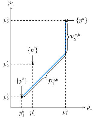
(a) Sets playing a role in the definition of $\mathcal{P}^{*}$

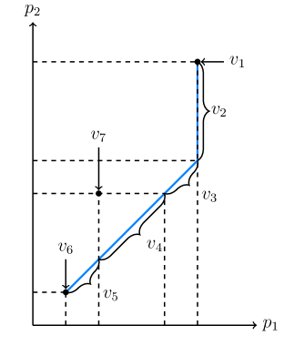
(b) $\mathcal{V}\equiv\{v_{1},\ldots,v_{7}\}$ satisfying Definition V

To better understand the various sets of prices, Figure 1(a) first graphically illustrates those in (18)-(20) in the context of an example with three alternatives. Figure 1(b) then illustrates a partition of the union of the sets in Figure 1(a) to obtain a collection of sets satisfying Definition V. In particular, it breaks up any two sets in Figure 1(a) that partially overlap in a given coordinate such that Definition V(iii) is satisfied. In Appendix LABEL:S-sec:procedure_V, we formally describe how the partition can more generally be obtained in such a manner.

Using $\mathcal{V}$, we can now construct our $\mathcal{W}$. To this end, observe first that for each $j\in\mathcal{J}$, the collection of sets determined by the prices in $v\in\mathcal{V}$ in the $j$th coordinate, i.e. $\left\{v_{[j]}:v\in\mathcal{V}\right\}$, generates a partition of $\left[p_{j}^{b},p_{j}^{a}\right]\cup\{p_{j}:\mathcal{P}_{\text{obs}}\}\subseteq[\underline{p}_{j},\bar{p}_{j}]$. Moreover, observe that the collection of intervals between the observed price values outside $\left[p_{j}^{b},p_{j}^{a}\right]$, i.e. $\left\{\left[\underline{p}_{j},\underline{p}_{1,j}^{*}\right)\right\}\cup\left\{\left(\underline{p}_{m-1,j}^{*},\underline{p}_{m,j}^{*}\right)\right\}_{m=2}^{\underline{M}_{j}}\cup\left\{\left(\bar{p}_{m-1,j}^{*},\bar{p}_{m,j}^{*}\right)\right\}_{m=2}^{\overline{M}_{j}}\cup\left\{\left(\bar{p}_{\bar{M}_{j},j}^{*},\bar{p}_{j}\right]\right\}$ where $\underline{p}^{*}_{1,j}\leq\ldots\leq\underline{p}^{*}_{\underline{M}_{j},j}$ and $\bar{p}^{*}_{1,j}\leq\ldots\leq\bar{p}^{*}_{\overline{M}_{j},j}$ are the ordered values of $\{p_{j}:p\in\mathcal{P}_{\text{obs}},~{}p_{j}\leq p^{b}_{j}\}\cup\{p^{b}_{j}\}$ and $\{p_{j}:p\in\mathcal{P}_{\text{obs}},~{}p_{j}\geq p^{a}_{j}\}\cup\{p^{a}_{j}\}$, respectively, generates a partition of $[\underline{p}_{j},\bar{p}_{j}]\setminus\left(\left[p_{j}^{b},p_{j}^{a}\right]\cup\{p_{j}:\mathcal{P}_{\text{obs}}\}\right)$. In turn, we together have that

$$\mathcal{V}_{j}\equiv \left\{\left[\underline{p}_{j},\underline{p}_{1,j}^{*}\right)\right\}\cup\left\{\left(\underline{p}_{m-1,j}^{*},\underline{p}_{m,j}^{*}\right)\right\}_{m=2}^{\underline{M}_{j}}\cup\left\{v_{[j]}\right\}_{v\in\mathcal{V}}\cup\left\{\left(\bar{p}_{m-1,j}^{*},\bar{p}_{m,j}^{*}\right)\right\}_{m=2}^{\overline{M}_{j}}\cup\left\{\left(\bar{p}_{j}^{*},\bar{p}_{j}\right]\right\}$$ (22)

generates a partition of $[\underline{p}_{j},\bar{p}_{j}]$, i.e. the space of prices along the $j$th coordinate. We then take $\mathcal{W}$ to be the Cartesian product of $\mathcal{V}_{j}$ across the different coordinates, i.e.

$$\mathcal{W}=\prod_{j\in\mathcal{J}}\mathcal{V}_{j}\equiv\left\{w_{1},\ldots,w_{M}\right\}~{}.$$ (23)

It is useful to highlight that our construction of $\mathcal{W}$ simplifies in the case where demand is unidimensional—essentially arising when all alternatives except one have prices normalized to 0. As noted in Section 1.1, this special case is similar to the identification problem studied in Bhattacharya (2021) and Mogstad et al. (2018), who propose a finite dimensional space of functions comparable to that in (17) as a solution. In this case, we do not require to impose $\mathcal{V}$ to additionally satisfy Definition V(iii) as it is automatically implied by the fact that $\mathcal{V}$ is a partition. In contrast, in the multidimensional case, this is not the case and, hence, we need to explicitly introduce it to ensure that the information provided by the shape restrictions in (13) is preserved. Moreover, given $\mathcal{V}$, the construction of $\mathcal{W}$ follows more straightforwardly in the unidimensional case as the sets in $\mathcal{V}$ and those outside it, i.e. those in (22), directly generate a partition of the space of prices for a single coordinate. For the multidimensional case, an additional complication remains of how to combine these one dimensional partitions to partition the entire space of prices, which we propose to solve by taking their Cartesian product as in (23).

3.1.2 Equivalent Finite Dimensional Characterization

Given our constructed $\mathcal{W}$, we next show that replacing the infinite-dimensional $\mathbf{Q}_{B}$ with the finite-dimensional $\mathbf{Q}^{\text{fd}}_{B}$ in (17) leads to no loss of information, i.e. $\theta\left(\mathbf{Q}_{B}\right)=\theta\left(\mathbf{Q}^{\text{fd}}_{B}\right)$. Furthermore, we show that $\theta\left(\mathbf{Q}^{\text{fd}}_{B}\right)$ can be computed by two finite-dimensional optimization problems.

In order to state this result, it is useful to first rewrite $\theta\left(\mathbf{Q}^{\text{fd}}_{B}\right)$ in terms of $\beta\equiv\left(\beta^{\prime}_{j}:j\in\mathcal{J}\right)^{\prime},$ where $\beta_{j}=\left(\beta_{j}(w_{1}),\ldots,\beta_{j}(w_{M})\right)$, i.e. the variable parameterizing $q\in\mathbf{Q}^{\text{fd}}_{B}$. To this end, observe that given $\theta$ is continuous in $q$ and that $q$ is continuous in $\beta$, there exists a continuous function $\theta_{B}$ of $\beta$ such that $\theta(q)=\theta_{B}(\beta)$. Similarly, observe that $\mathbf{Q}_{B}$ can also be written in terms of $\beta$ by

$$\mathbf{B}=\left\{\beta\in\mathbf{R}^{d_{\beta}}:\left(\sum_{w\in\mathcal{W}}1_{w}\cdot\beta_{j}(w):j\in\mathcal{J}\right)\in\mathbf{Q}_{B}\right\}~{},$$ (24)

where $d_{\beta}$ denotes the dimension of $\beta$, i.e. the set of values of $\beta$ that ensure that the corresponding $q$ is in $\mathbf{Q}_{B}$. Then, we can write $\theta\left(\mathbf{Q}^{\text{fd}}_{B}\right)$ in terms of $\beta$ by

$$\left\{\theta_{0}\in\mathbf{R}:\theta_{B}(\beta)=\theta_{0}\text{ for some }\beta\in\mathbf{B}\right\}\equiv\Theta_{B}~{}.$$ (25)

In the following proposition, we show that $\theta\left(\mathbf{Q}_{B}\right)$ is equal to $\Theta_{B}$, and that $\Theta_{B}$ can be computed by two finite-dimensional optimization problems.

Proposition 2.

Suppose that $\mathbf{Q}=\mathbf{Q}_{B}$. Then, the identified set in (10) is equal to that in (25), i.e. $\Theta=\Theta_{B}$. In addition, if $\mathbf{B}$ is empty then by definition $\Theta_{B}$ is empty; whereas, if $\mathbf{B}$ is non-empty then $\Theta_{B}=[\underline{\theta}_{B},\bar{\theta}_{B}]$, where

$$\underline{\theta}_{B}=\min_{\beta\in\mathbf{B}}~{}\theta_{B}(\beta)~{}\text{ and }~{}\bar{\theta}_{B}=\max_{\beta\in\mathbf{B}}~{}\theta_{B}(\beta)~{}.$$ (26)

Proposition 2 shows that the identified set when not empty is given by a closed interval, where the endpoints can be obtained by solving two optimization problems. In the proof of the proposition, we explicitly derive $\mathbf{B}$, the constraint set of these optimization problems, and observe that it is determined by constraints that are all linear in $\beta$. We also derive $\theta_{B}$, the objectives of these optimization problems, and observe that it is linear in $\beta$. These two observations then imply that the optimization problems are linear programs, a useful observation in their implementation. Lastly, observe that to compute the identified set using these linear programs, we specifically require that $\mathbf{B}$ is non-empty or, equivalently, that the model is correctly misspecified. However, when this is not the case, the linear programs automatically terminate.

3.1.3 Dimension Reduction

While the problems in (26) are linear programs, they can nonetheless be computationally expensive when the dimension of the optimizing variable $\beta$ is large. Such a case arises especially when $|\mathcal{J}|$ is large as in our application where it is equal to 70. To ensure tractability in such cases, we conclude this subsection by considering two lower-dimensional linear programs that are easier to compute and can continue to allow us to learn about our parameter.

Our first proposal considers sub-programs of (26) that obtain outer sets containing $\Theta_{B}$. In particular, given how $\mathcal{V}$ how was constructed, observe that the following subset of $\mathcal{W}$

$$\mathcal{W}^{\text{r}}=\left\{w\in\mathcal{W}:w=\prod_{j\in\mathcal{J}}v_{[j]}\text{ for some }v\in\mathcal{V}\right\}\equiv\left\{w^{\text{r}}_{1},\ldots,w^{\text{r}}_{M^{\text{r}}}\right\}~{},$$

captures the sets of prices that play a role in the definition of the parameter, and in turn the subvector of $\beta$ defined over these sets given by $\beta^{\text{r}}=\left(\beta^{\text{r}^{\prime}}_{j}:j\in\mathcal{J}\right)^{\prime}\equiv\phi(\beta)$, where $\beta^{\text{r}}_{j}=\left(\beta_{j}(w^{\text{r}}_{1}),\ldots,\beta_{j}(w^{\text{r}}_{M^{\text{r}}})\right)$, is sufficient in determining $\theta_{B}$ in the sense that there exists a linear function $\theta_{B}^{\text{r}}$ such that $\theta_{B}^{\text{r}}(\beta^{\text{r}})=\theta_{B}(\beta)$. The lower-dimensional linear programs we consider are those in terms of the subvector $\beta^{\text{r}}$ given by

$$\underline{\theta}_{B}^{\text{r}}=\min_{\beta^{\text{r}}\in\mathbf{B}^{\text{r}}}~{}\theta^{\text{r}}_{B}(\beta^{\text{r}})~{}\text{ and }~{}\bar{\theta}_{B}^{\text{r}}=\max_{\beta^{\text{r}}\in\mathbf{B}^{\text{r}}}~{}\theta^{\text{r}}_{B}(\beta^{\text{r}})~{},$$ (27)

where $\mathbf{B}^{\text{r}}$ denotes a set of $\beta^{\text{r}}$ determined by linear constraints. Indeed, if $\mathbf{B}^{\text{r}}=\phi(\mathbf{B})$, we have by construction that these programs are equivalent to those in (26). In turn, by taking $\mathbf{B}^{\text{r}}$ to be such that $\phi(\mathbf{B})\subseteq\mathbf{B}^{\text{r}}$, it follows that we have $\underline{\theta}_{B}^{\text{r}}\leq\underline{\theta}_{B}$ and $\bar{\theta}_{B}^{\text{r}}\geq\bar{\theta}_{B}$, and hence obtain an outer set for $\Theta_{B}$, i.e. $\Theta_{B}\in\left[\underline{\theta}_{B}^{\text{r}},\bar{\theta}_{B}^{\text{r}}\right]$. In Appendix LABEL:S-sec:B_r, we provide a natural choice of such a $\mathbf{B}^{\text{r}}$ determined by restrictions on $\beta^{\text{r}}$ implied by those in $\mathbf{B}$, which we find in our empirical analysis can be tractably implemented and result in informative conclusions.

Our second proposal is to additionally impose separability on the demand functions given which we can sharply compute the identified set in tractable manner. In our empirical analysis, we specifically consider the following separability assumption that imposes that demand is a sum of lower-dimensional functions:

Assumption S.

(Separability)  For each $j\in\mathcal{J}$, $q_{j}(p)=\sum\limits_{m\in\mathcal{J}}h_{jm}(p_{m})$ for some unknown functions $\{h_{jm}:m\in\mathcal{J}\}$.

Assumption S imposes the demand for each alternative to be additively separable in prices of all the alternatives. In Appendix LABEL:S-sec:separability, we consider a more general separability assumption and show how Proposition 2 can be extended such that we can similarly use two linear programs as in (26) to compute the identified set under these additional assumptions. Importantly, we also highlight here that by requiring demand to be composed of lower dimension functions, the dimension of the optimizing variable in these programs can be substantially smaller than those in (26).

3.2 Identified Set under Auxiliary Parametric Specification

3.2.1 Characterization

In contrast to the nonparametric specification, the problem in the auxiliary specification is finite-dimensional in nature due to the fact that $\mathbf{Q}_{A}$ is a finite-dimensional parameterized space. In this case, $\theta(\mathbf{Q}_{A})$ can hence be directly characterized by searching over $q$ in $\mathbf{Q}_{A}$ and then taking their image under the function $\theta$.

In order to state the result that shows how to do this, it is useful as before to first rewrite $\theta(\mathbf{Q}_{A})$ in terms of $\alpha$, i.e. the variable parameterizing $q\in\mathbf{Q}_{A}$ through (15). Observe that given $\theta$ is continuous in $q$ and that $q$ is continuous in $\alpha$, there exists a continuous function $\theta_{A}$ of $\alpha$ such that $\theta(q)=\theta_{A}(\alpha)$. Similarly, observe that $\mathbf{Q}_{A}$ can also be written in terms of $\alpha$ by

$$\mathbf{A}=\left\{\alpha\in\mathbf{R}^{d_{\alpha}}:\left(\sum_{k=0}^{K_{j}}\alpha_{jk}\cdot b_{jk}:j\in\mathcal{J}\right)\in\mathbf{Q}_{B}\right\}~{}.$$ (28)

where $d_{\alpha}$ denotes the dimension of $\alpha$, i.e. the set of values of $\alpha$ that ensure that the corresponding $q$ is in $\mathbf{Q}_{B}$. Then, we can write $\theta(\mathbf{Q}_{A})$ in terms of $\alpha$ by

$$\theta_{A}(\mathbf{A})=\left\{\theta_{0}\in\mathbf{R}:\theta_{A}(\alpha)=\theta_{0}\text{ for some }\alpha\in\mathbf{A}\right\}\equiv\Theta_{A}~{}.$$ (29)

In the following proposition, we show that when $\mathbf{A}$ is connected and non-empty, the closure of $\Theta_{A}$ is equal to an interval, where the endpoints can be characterized as solutions to two finite-dimensional optimization problems.

Proposition 3.

If $\mathbf{A}$ is empty then by definition $\Theta_{A}$ is empty; whereas, if $\mathbf{A}$ is connected and non-empty, then the closure of $\Theta_{A}$ is given by $[\underline{\theta}_{A},\bar{\theta}_{A}]$, where

$$\underline{\theta}_{A}=\inf_{\alpha\in\mathbf{A}}~{}\theta_{A}(\alpha)~{}\text{ and }~{}\bar{\theta}_{A}=\sup_{\alpha\in\mathbf{A}}~{}\theta_{A}(\alpha)~{}.$$ (30)

3.2.2 Polynomial Specifications

Proposition 3 shows how to characterize the identified set under a general class of parametric restrictions. In our empirical analysis, for computational tractability, we consider parsimonious specifications that are parameterizations of the separable functions in Assumption S. In particular, we consider

$$q_{j}(p)=\sum\limits_{m\in\mathcal{J}}\sum_{k=0}^{K}\alpha_{jmk}\cdot p_{m}^{k}$$ (31)

for each $j\in\mathcal{J}$ and some unknown parameters $\left\{\alpha_{jmk}:m\in\mathcal{J},~{}0\leq k\leq K\right\}$, i.e. where the unknown functions in Assumption S are assumed to be polynomials of degree $K$.

While the optimization problems in (30) are finite-dimensional, their computational tractability depends on the structure of the objective $\theta_{A}$ and the constraint set $\mathbf{A}$. In Appendix LABEL:S-sec:bernstein, we illustrate that under (31), $\theta_{A}$ is a linear function of $\alpha$ and that $\mathbf{A}$ is characterized by linear equality and inequality restrictions on $\alpha$. However, we observe here that some of the linear restrictions are evaluated at every price in the continuous space $\mathcal{P}$, which implies that the resulting optimization problems can be generally difficult to compute. To this end, we consider the following alternative optimization problems

$$\underline{\theta}_{A}^{\text{r}}=\min_{\alpha\in\mathbf{A}^{\text{r}}}\theta_{A}(\alpha)~{}\text{ and }~{}\bar{\theta}_{A}^{\text{r}}=\max_{\alpha\in\mathbf{A}^{\text{r}}}\theta_{A}(\alpha)~{}$$ (32)

in our empirical analysis, where $\mathbf{A}^{\text{r}}$ corresponds to a subset of $\mathbf{A}$ that evaluates some of the restrictions on only a finite set of prices in $\mathcal{P}$—the exact form of $\mathbf{A}^{\text{r}}$ is provided in Appendix LABEL:S-sec:bernstein. As the objective and the finite number of restrictions determining the constraint sets of these problems are linear in $\alpha$, they are linear programs and hence generally computationally tractable. But, since $\mathbf{A}\subseteq\mathbf{A}^{\text{r}}$, these problems only provide an outer set for $\Theta_{A}$, i.e. $\Theta_{A}\subseteq[\underline{\theta}_{A}^{\text{r}},\bar{\theta}_{A}^{\text{r}}]$, similar in spirit to those in (27) with respect to $\Theta_{B}$.

4 Evaluation of the DC Opportunity Scholarship Program

4.1 Background

The DC Opportunity Scholarship Program (OSP) was a federally-funded school voucher program established by Congress in January 2004, and which started accepting students for the 2004-2005 school year. The OSP was structured similarly to other voucher programs that existed at the time (Epple et al., 2017). It was open to students residing in Washington, DC, and whose family income was no higher than 185% of the federal poverty line ($18,850 for a family of four in 2004). It could be used only for K-12 education, and at the time of initial receipt was renewable for up to five years. It provided students a voucher worth $7,500 that could be used to offset tuition, fees, and transportation at any private school of their choice participating in the program.

The law that established the program also mandated its evaluation, which culminated with a final report to Congress (Wolf et al., 2010). The report exploited the fact that the OSP randomly allocated vouchers to participating students. In particular, Congress expected the program to be oversubscribed, i.e. the number of applicants would exceed the number of available vouchers. As a result, it required that vouchers be randomly allocated to applicants through a lottery if the program was oversubscribed—see Wolf et al. (2010) for details on the lottery. Wolf et al. (2010) exploited this random allocation by comparing various outcomes of voucher recipients to non-recipients to experimentally evaluate the effect of voucher receipt on these outcomes. The main findings, as listed in the executive summary, can be broadly summarized as follows. First, they find no conclusive evidence that the receipt of the voucher had any significant effects on various outcomes corresponding to student achievement. Second, they find that the receipt of the voucher significantly improved students’ chances of graduating from high school. Finally, they find that the receipt of the voucher raised parents’ ratings of school safety and satisfaction.

In what follows, we use the tools developed in the previous sections to complement these findings by analyzing the welfare effects of the price subsidy induced by the status quo voucher amount as well as counterfactual amounts. Our analysis is motivated by the fact that while the receipt of the voucher revealed mixed evidence on outcomes in the sense that there are zero as well as some positive effects, parents may nonetheless value the voucher, potentially across dimensions not easily captured by the outcomes. Indeed, as highlighted below, the data reveals that a non-trivial proportion of voucher recipients used the voucher, which, by revealed preference arguments, implies that they value receiving the voucher. Our analysis estimates these potential welfare benefits using data collected by the OSP.

4.2 Setting

In the context of our setup in Section 2, let $D_{i}$ correspond to the enrolled school and let it take values in $\mathcal{J}=\mathcal{J}_{v}\cup\{g,n\}$, where $\mathcal{J}_{v}$ denotes the set of private schools in the program, and $g$ and $n$ denote alternatives of enrolling in a government school (which includes charter schools) and a private school not in the program, respectively. In order to define the support of the price vector $P_{i}$, note that the voucher affected only the prices (tuition) of private schools in the program, and hence there is no variation in the prices of government and private schools not in the program. The prices of the alternatives $g$ and $n$ are therefore normalized to zero. For the private schools in the program, the variation in prices is determined by the receipt of the status quo voucher. For each $j\in\mathcal{J}_{v}$, let $p^{*}_{j}\in\mathbf{R}_{+}$ denote the original price of the school, and let $p_{j}(\tau)=\max\{p^{*}_{j}-\tau,0\}$ denote its price under the application of a voucher of amount of $\tau\in\mathbf{R}_{+}$, as the voucher provided an amount of at most $\tau$ to cover tuition. Moreover, let $p(\tau)=(p_{j}(\tau):j\in\mathcal{J})$ denote the vector of prices under a voucher amount of $\tau\in\mathbf{R}_{+}$, where note that $p_{g}(\tau)=p_{n}(\tau)=0$ as their prices are normalized to 0. Denoting by $\tau_{\text{sq}}$ the status quo amount, the support of the prices is then given by $\mathcal{P}_{\text{obs}}=\{p(0),p(\tau_{\text{sq}})\}$, i.e. the prices with and without the status quo voucher. Given that the voucher was randomly assigned to students, we have that Assumption E is satisfied.

The objective of our empirical analysis is to learn the welfare effects of the price decrease induced by the voucher, i.e. (5) when $p^{a}=p(0)$ and $p^{b}=p(\tau)$ given by

$$AB(\tau)\equiv E[B_{i}^{a,b}]~{}.$$ (33)

Indeed, when $\tau=\tau_{\text{sq}}$, this corresponds to the effect of providing the status quo voucher amount, while when $\tau\neq\tau_{\text{sq}}$, it corresponds to the effect of providing a counterfactual voucher amount. To benchmark these benefits and perform a cost-benefit analysis, we also study additional parameters that measure the costs the government may face when individuals receive the voucher net of those when they do not receive it, which can be straightforwardly written as (7). In particular, denoting by $\{c_{j}(\tau):j\in\mathcal{J}\}$ the costs that the government associates with enrollment in the different alternatives under a voucher of amount $\tau$, we take the average cost of the voucher to be

$$AC(\tau)=\sum_{j\in\mathcal{J}}c_{j}(\tau)q_{j}(p(\tau))-c_{j}(0)q_{j}(p(0))~{},$$ (34)

and the average surplus measuring benefit net of cost by

$$AS(\tau)=AB(\tau)-AC(\tau)~{}.$$ (35)

We take $c_{g}(\tau)=c_{g}$, i.e. the cost associated with government schools is some known value $c_{g}$; $c_{n}(\tau)=0$, i.e. the cost associated with private schools not in the program is zero; and $c_{j}(\tau)=\min\{p_{j}(0),\tau\}+\mu\cdot 1\{\tau>0\}$, i.e. the cost associated with private schools in the program is the voucher amount spent to cover tuition plus some known administrative cost $\mu$ of operating the program (i.e. charged only when the voucher amount is positive). For the known values, we take $c_{g}=\$$5,355, which corresponds to the educational expenditure reported by the US Census (2005). This is lower than total per-pupil expenditure from the Census ($12,979, which includes some fixed costs), or educational expenditure as measured in other sources ($8,105, Sable and Hill (2006)). However, as our surplus parameter is increasing in $c_{g}$, we choose the smaller, more conservative value. On the other hand, we take $\mu=\$200$, which corresponds to cost of administration, adjudication and providing information to families for an alternative school voucher program reported in Levin and Driver (1997)—see Figure LABEL:S-fig:AS_cost for robustness to a range of other values of $c_{g}$ and $\mu$.

It is useful to highlight some limitations of our setup and how it affects the interpretation of our subsequent results. As noted in Section 2.1, our model does not capture channels through which the voucher may affect choice beyond a decrease in prices. Examples of such channels noted previously in the literature primarily correspond to various general equilibrium effects that affect utilities under different schools due to changes in school incentives to invest in quality (Allende, 2019; Neilson, 2013) or changes in peer composition (Allende, 2019; Gazmuri, 2019). Indeed, capturing such channels requires a richer model that explicitly introduces them in its structure. Our analysis can therefore more appropriately be viewed as a partial equilibrium one that takes these channels as fixed. More concretely, it can be viewed as analyzing the effects of a marginal policy that provides a voucher to an additional student who applied to the OSP but was not admitted, rather than those of scaling up the program that may induce general equilibrium effects.

Moreover, recall that our analysis relies on the expression for the average willingness to pay in Proposition 1, which requires the underlying utilities to be continuous in disposable income. In our empirical setting, this assumption, however, can potentially be suspect. As elaborated in Appendix LABEL:S-sec:liquidity, this is due to the fact that individuals may be liquidity constrained and hence whether they can afford to choose an alternative may discontinuously change with its price. In Proposition LABEL:S-prop:liquidity, we extend Proposition 1 to show that in this case the expression in (6) continues to conservatively provide a valid lower bound for the average willingness to pay—the upper bound can intuitively go to infinity as the price decrease can make a new alternative affordable and hence is similar to an infinite price decrease that individuals may have an unbounded willingness to pay for. In this sense, our analysis can be conservatively viewed as providing a lower bound for the welfare effects. As we will observe below, our empirical conclusions are primarily based on the lower bounds of our estimates and therefore remain robust to this feature.

4.3 Data and Summary Statistics

The OSP collected detailed data for the first two years of the program, 2004 and 2005, and tracked students for at least four years. Across these years, the composition of applicants and private schools in the program changed. To keep prices and the set of eligible schools the same for all students, we focus on the second year of the program, 2005, which contains around $80\%$ of the entire sample. In addition, to avoid complications from dynamics, we focus on the initial year of the data for students entering the program this year. In Appendices LABEL:S-sec:data_construction-LABEL:S-sec:summstat_setting, we provide details on how our analysis sample was constructed from the original evaluation data as well as various statistics on the schools and sample of individuals. Below, we present summary statistics for the main variables our analysis exploits, namely the enrollment shares and the prices of private schools in the program.

Table 1: Enrollment shares across school type by voucher receipt

With voucher Without Voucher Difference Government schools 0.288 0.901 -0.613 [0.453] [0.299] (0.018) Private schools not in program 0.014 0.020 -0.006 [0.117] [0.140] (0.006) Private schools in program 0.698 0.079 0.619 [0.459] [0.270] (0.018) Observations 1,090 730 • Observations rounded to the nearest 10. Standard deviations in square brackets and robust standard errors in parentheses. • SOURCE: Evaluation of the DC Opportunity Scholarship Program: Final Report (NCEE 2010-4018), U.S. Department of Education, National Center for Education Statistics previously unpublished tabulations.

Table 1 presents enrollment shares across the three types of schools, i.e. government schools and private schools in and not in the program, by voucher receipt. A relatively large proportion (69.8$\%$) choose to take up the voucher as revealed by those enrolled in private schools in the program. By revealed preference, this implies that recipients value the voucher. In addition, the voucher increases the proportion enrolling in voucher private schools by 61.9 percentage points, suggesting that prices play an important role in inducing private school enrollment. The voucher also produces a nearly symmetric decline in the proportion enrolled in government schools (-61.3 percentage points) implying that nearly all students induced into voucher schools would be in government ones absent the voucher.

Figure 2: Tuition prices across voucher private schools, and enrollment shares across them as well as government and non-voucher private schools.

SOURCE: Evaluation of the DC Opportunity Scholarship Program: Final Report (NCEE 2010-4018), U.S. Department of Education, National Center for Education Statistics previously unpublished tabulations.

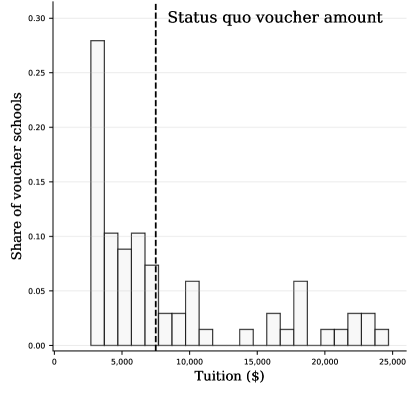
(a) Tuition of private schools in the program

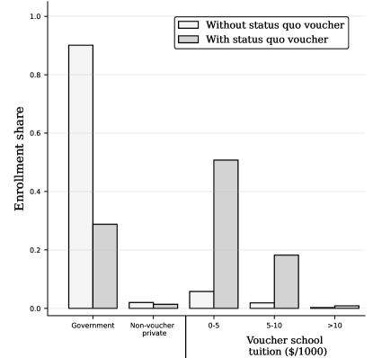
(b) Enrollment shares

In 2005, there were approximately 70 private schools in the program (out of a total of about 110 in Washington, DC). Figure 2 summarizes the variation in prices across these schools as well as the enrollment shares across various ranges of these prices. Figure 2(a) reveals that a large number of voucher schools had low prices—around 80$\%$ had prices below the status quo voucher amount. Figure 2(b) reveals that the voucher induced a significant proportion to enroll in these low-price schools—out of the 61.9 percentage point increase in the proportion attending a voucher private school, a full 59 percentage points (95%) was into schools with prices less than the status quo voucher amount. Similarly, a large proportion of recipients (81$\%$) redeem the voucher at schools with prices below the cost of a government school. Given that the majority of these recipients would have enrolled in government schools absent the voucher as observed from Table 1, this suggests that the government may face only small net costs or even savings from the provision of a voucher. Our estimates below make this point more precisely.

4.4 Welfare Estimates

Table 2: Estimated bounds and 90$\%$ confidence intervals on welfare effects for status quo voucher amount

Nonparametric (NP) Parametric (P) Separable, $K$ Baseline Separable 1 2 3 4 5 (1) (2) (3) (4) (5) (6) (7) 156 156 1,583 1,011 723 541 403 $AB(\tau_{\text{sq}})$ 362 362 1,752 1,168 891 710 585 5,239 3,344 1,853 2,426 2,752 2,952 3,114 5,570 3,587 1,996 2,607 2,958 3,171 3,333 -168 -168 -168 -168 -168 -168 -168 $AC(\tau_{\text{sq}})$ 113 113 113 113 113 113 113 332 332 332 332 332 332 332 80 80 1,433 873 610 428 303 $AS(\tau_{\text{sq}})$ 249 249 1,639 1,055 778 597 472 5,126 3,231 1,740 2,313 2,639 2,839 3,001 5,557 3,512 1,921 2,519 2,870 3,083 3,245 • For each parameter, the inner panel reports the estimated bounds and the outer panel reports confidence intervals, respectively. Lower and upper bounds are not repeated if they coincide. • SOURCE: Evaluation of the DC Opportunity Scholarship Program: Final Report (NCEE 2010-4018), U.S. Department of Education, National Center for Education Statistics previously unpublished tabulations.

Table 2 presents estimated bounds for the welfare effects of providing the status quo voucher amount. Each row corresponds to the parameters in (33)-(35) taking $\tau=\tau_{\text{sq}}\equiv\$7,500$. Each column corresponds to a specification of demand, which is either the baseline nonparametric specification, or when separability in Assumption S or their parameterized version in (31) for some value of $K$ is imposed. We consider $K$ from 1 to 5. Here and in the remainder of the empirical analysis, bounds under the nonparametric baseline specification are estimated using (27) with the choice of $\mathbf{B}^{\text{r}}$ described in Appendix LABEL:S-sec:B_r, those under nonparametric separability assumptions are estimated using (LABEL:S-eq:bounds_opt_S) described in Appendix LABEL:S-sec:separability, and those under the parametric specifications are estimated using (32) with choices of $\mathbf{A}^{\text{r}}$ described in Appendix LABEL:S-sec:bernstein, where in all cases the enrollment shares in the restriction in (8) are replaced by their empirical counterparts. We also report 90$\%$ confidence intervals, which are constructed using a bootstrap procedure from Bugni et al. (2017) described in Appendix LABEL:S-sec:inference.

The estimates for $AB\left(\tau_{\text{sq}}\right)$ under the baseline nonparametric specification in Column (1) reveal that the average benefit from the status quo voucher can range between $\$$362 and $\$$5,239. While these bounds are potentially not sharp as noted in Section 3.1.3, comparing them to the sharp ones under the separability assumption in Column (2) reveal that the lower bounds are equal and hence that at least the lower bound is sharp. The estimates for $AC\left(\tau_{\text{sq}}\right)$ reveal that it is point identified. This is because it is a function of demand at values of prices observed in the data, namely the prices with and without the status quo voucher. The average cost, equal to $\$113$, is low compared to the amount of $\$$7,500 that the voucher provides. As highlighted above, this is due to the fact that a large proportion of recipients redeem the voucher at low-cost private schools relative to government schools they would have enrolled absent the voucher.

Taking the difference between benefits and costs, the estimates for $AS\left(\tau_{\text{sq}}\right)$ reveal that the average benefit net of costs of the status-quo voucher is positive. Importantly, this finding robustly holds even under the nonparametric baseline specification in which case the net benefit is at least $\$$249. Moreover, from the upper bounds, we can observe that a potentially high net benefit is consistent with the data, where they can range from $\$$1,740 to $\$$5,126 depending on the strength of assumptions one is willing to impose. Overall, this suggests that the voucher recipients can have a large welfare benefit from the private schools at which they redeem the voucher relative to the costs the government faces to fund the voucher at these schools. The confidence intervals reveal that these findings are also statistically significant.

Figure 3: Estimated bounds on welfare effects for a range of voucher amounts

SOURCE: Evaluation of the DC Opportunity Scholarship Program: Final Report (NCEE 2010-4018), U.S. Department of Education, National Center for Education Statistics previously unpublished tabulations.

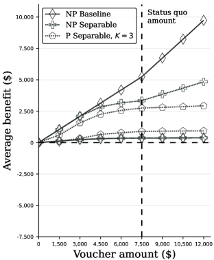
(a) $AB(\tau)$

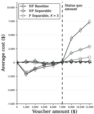
(b) $AC(\tau)$

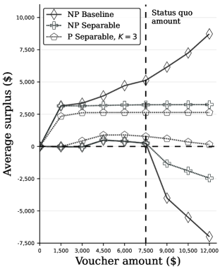
(c) $AS(\tau)$

Figure 3 presents estimated bounds for the parameters in (33)-(35) for a range of counterfactual voucher amounts beyond the status quo, for the baseline and separable nonparametric specification as well as the parametric specification from Column (5) in Table 2. As in the case of the status quo, for values below the status quo amount, Figure 3(c) reveals that under the baseline specification we continue to robustly find positive, potentially large net benefits—Figure LABEL:S-fig:AS_tau_ci reveals that this finding is also generally statistically significant. However, for those above the status quo amount, the conclusion on the presence of positive effects is dependent on the strength of the assumptions. In particular, we have positive net benefits only if we are willing to impose parametric restrictions in which case the net benefits are positive for a range of values above the status quo amount.

This can be explained from the estimates of the underlying average benefits and cost in Figures 3(a) and (b). In both figures, the bounds for the nonparametric specification appear to be significantly tighter for values of the voucher below the status quo rather than those above it. Intuitively, this is because, in contrast to the parametric specification, the nonparametric specifications allow for much more flexibility in the substitution patterns between schools and also, in contrast to values of the voucher below the status quo, there is no additional data at higher voucher amounts to provide information on the potential substitution patterns. In turn, the bounds are wide, highlighting that a range of patterns are nonparametrically consistent with the data.

4.5 Role of Low-Tuition Schools

In summary, our welfare estimates reveal that voucher provision has positive, potentially large net benefits under the status quo as well as a range of counterfactual voucher amounts. While discussing our results above, we highlighted that the positive effects arose in part due to the presence of low-tuition schools in the program that many recipients attend, but that have a small net cost to the government. We conclude our analysis by further exploring the importance of these schools in the program under the status quo voucher amount.

We analyze how our estimates change when we remove schools having prices less than a certain amount from the program. For a given $\kappa\in\mathbf{R}_{+}$, let $\mathcal{J}^{\kappa}=\{j\in\mathcal{J}_{v}:p_{j}(0)\leq\kappa\}$ denote the set of private schools in the program with prices no more than $\kappa$, and let $p^{\kappa}_{j}(\tau)$ be equal to $p_{j}(0)$ if $j\in\mathcal{J}^{\kappa}$ and $p_{j}(\tau)$ otherwise, i.e. the voucher amount is applied to only schools with prices above $\kappa$. Then we are interested in studying the parameter in (5) when $p^{a}=p(0)$ and $p^{b}=p^{\kappa}(\tau)$,

$$AB^{\kappa}\left(\tau_{\text{sq}}\right)\equiv E[B_{i}^{a,b}]~{},$$ (36)

as well as analogous versions of those in (34) and (35) given by

$$AC^{\kappa}\left(\tau_{\text{sq}}\right) =\sum_{j\in\mathcal{J}}c^{\kappa}_{j}(\tau_{\text{sq}})\cdot q_{j}(p^{\kappa}(\tau_{\text{sq}}))-\sum_{j\in\mathcal{J}}c_{j}(0)\cdot q_{j}(p(0))~{},$$ (37)

$$AS^{\kappa}\left(\tau_{\text{sq}}\right) =AB^{\kappa}\left(\tau_{\text{sq}}\right)-AC^{\kappa}\left(\tau_{\text{sq}}\right)~{},$$ (38)

where $c_{j}^{\kappa}(\tau_{\text{sq}})=c_{j}(\tau_{\text{sq}})$ for $j\in\mathcal{J}\setminus\mathcal{J}^{{}^{\kappa}}$ and $c_{j}^{\kappa}(\tau_{\text{sq}})=0$ for $j\in\mathcal{J}^{\kappa}$, i.e. we take the same costs as that in (34) except with the difference that we take the schools that are removed from the program to have zero costs.

Figure 4 presents estimated bounds for a range of values of $\kappa$. Intuitively, as the baseline nonparametric specification imposes no restriction on substitution patterns and as the data provides no information on variation where the voucher is applied to only certain voucher schools, the bounds under the baseline nonparametric specification can be wide. The bounds under the parametric specification in contrast can be substantially smaller. Across all specifications, Figure 4(c) suggests that the removal of low-tuition schools from the program generally results in the reduction of average surplus. Importantly, it reveals that removing schools with tuition of $\$$3,500 and lower from the program could potentially cause it to have a negative surplus. A closer look at Figure 2(a) reveals that nearly 30% of schools in the program have tuition of at most this value. The estimates reveal that the presence of these low-tuition schools in the program plays an essential role in explaining the positive net benefits we find for the provision of the status quo voucher amount.

Figure 4: Estimated bounds on welfare effects when schools with tuition at most $\kappa$ are removed from the program

SOURCE: Evaluation of the DC Opportunity Scholarship Program: Final Report (NCEE 2010-4018), U.S. Department of Education, National Center for Education Statistics previously unpublished tabulations.

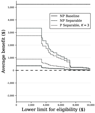
(a) $AB^{\kappa}\left(\tau_{\text{sq}}\right)$

(b) $AC^{\kappa}\left(\tau_{\text{sq}}\right)$

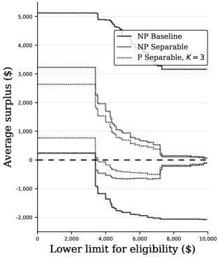
(c) $AS^{\kappa}\left(\tau_{\text{sq}}\right)$

To provide some suggestive evidence on what are the features of the low-tuition schools that are so compelling to voucher recipients, Table 3 compares various average characteristics between schools charging above and below $3,500 in tuition. Consistent with spending less money on instruction, the low-tuition schools have larger student-teacher ratios, and are somewhat less likely to have individual tutors or programs for students with learning difficulties. The most striking difference, however, is that they are much more likely to be Catholic—83% versus 16%. This suggests that voucher recipients particularly value this feature of low-tuition schools and is what drives their high welfare benefit for the voucher relative to the low cost of funding it at such schools.

Table 3: Average school characteristics by tuition level for voucher private schools

Tuition $\leq$ $\$$3,500 Tuition $>$ $\$$3,500 Difference School size 196.103 281.843 -85.740 Student/teacher ratio 13.000 9.860 3.140 Catholic (=1) 0.829 0.159 0.671 Other religious (=1) 0.003 0.256 -0.253 Gifted program (=1) 0.243 0.397 -0.155 Learning difficulties program (=1) 0.446 0.547 -0.101 Individual tutors available (=1) 0.609 0.774 -0.165 Students tracked by ability (=1) 0.763 0.729 0.034 Remedial classes available (=1) 0.646 0.619 0.027 Number of schools 20 50 • SOURCE: Evaluation of the DC Opportunity Scholarship Program: Final Report (NCEE 2010-4018), U.S. Department of Education, National Center for Education Statistics previously unpublished tabulations. Observations rounded to the nearest 10.

5 Comparison to Traditional Parametric Methods

In this section, we compare our empirical results and conclusions from the previous section to those we would obtain when applying traditional methods.

5.1 Logit Specifications

Recall from Section 2.3, our identification problem requires imposing restrictions on how the demand functions vary with price. Traditional methods do so by imposing a parametric functional form on demand such that it is point identified by the variation in the data, which in turn point-identifies our parameters of interest. These parametrizations are commonly implied by imposing functional forms on the utilities and parametric distributions on the unobserved heterogeneity.

In our comparison, we consider various versions of a standard logit parameterization of our model that begins by assuming

$$U_{ij}(Y_{i}-p_{j})=\xi_{j}-\gamma_{i}p_{j}+\epsilon_{ij}$$ (39)

for $j\in\mathcal{J}$, i.e utility is linear in prices, with alternative-specific intercepts, individual-specific price coefficients, and individual and alternative-specific shocks. The difference between the various versions arises from the distributions imposed on the unobserved heterogeneity $\gamma_{i}$ and $\epsilon_{ij}$ as follows:

1. Logit I: $\gamma_{i}=\bar{\gamma}_{0}$; and $\epsilon_{ij}$ is distributed independently across $j$ as Type I extreme value.

2. Logit II: $\gamma_{i}=\bar{\gamma}_{0}+\bar{\gamma}_{1}’X_{i}$; and $\epsilon_{ij}$ is distributed the same as in Logit I.

3. Mixed Logit: $\gamma_{i}=\bar{\gamma}_{0}+\bar{\gamma}_{1}’X_{i}+v_{i}$, where $v_{i}$ is normally distributed with mean 0 and variance $\sigma^{2}$; and $\epsilon_{ij}$ is distributed the same as in Logit I.

4. Nested Logit: $\gamma_{i}=\bar{\gamma}_{0}+\bar{\gamma}_{1}’X_{i}$; and $\epsilon_{i}=(\epsilon_{ij}:j\in\mathcal{J})$ has a CDF evaluated at $\epsilon$ equal to $\text{exp}\left(-\sum\limits_{k\in\{1,2\}}\left(\sum\limits_{j\in\mathcal{N}_{k}}e^{-\epsilon_{j}/\lambda_{k}}\right)^{\lambda_{k}}\right)$ for some $\lambda_{1},\lambda_{2}\in\mathbf{R}$, where $\mathcal{N}_{1}=\mathcal{J}_{v}\cup\{n\}$ and $\mathcal{N}_{2}=\{g\}$.

The first specification is a basic logit one that takes the price coefficient to be constant across individuals. The second and third respectively introduce observed and then unobserved heterogeneity in the price coefficient. The final specification introduces observed heterogeneity in the price coefficient, and dependence in the shocks across alternatives in the same nest, where there are two nests with one consisting of private schools and the other of government schools. Importantly, the flexibility of all these parameterizations is carefully chosen such that the underlying parameters are point identified given the binary variation in prices induced by the voucher, after imposing the usual location and scale normalizations—see, for example, Train (2009, Chapter 2.5). Table LABEL:S-tab:logit reports the parameter estimates for the various specifications, estimated using maximum likelihood. Here we take $X_{i}$ to be a vector of indicators for which bin the family income lies in, where there are four bins determined by quartiles of its empirical distribution.

As the underlying parameters are point identified, it follows that the corresponding demand functions are also point identified by plugging in the point identified parameter values in the expressions for demand implied by the various specifications—the expressions are provided in Table LABEL:S-tab:logit_exp. Similarly, as we do in what follows, we can estimate demand by plugging in the underlying parameter estimates from Table LABEL:S-tab:logit in the expressions in Table LABEL:S-tab:logit_exp, and then our parameters of interest by plugging in estimated demand in (7). In our implementation, the integrals with respect to $\phi$ in the expressions in Table LABEL:S-tab:logit_exp are numerically solved using simulation with 200 draws, while those with respect to $f_{X}$ are computed using the empirical distribution of $X_{i}$, and the integrals in the expression in (7) are numerically solved using a fine grid of points.

5.2 Observed and Counterfactual Demand Estimates

Before proceeding to the welfare estimates under the different logit specifications, we first present various estimates of the underlying demand functions implied by these specifications. In Figure 5(a), we analyze how well the implied demand functions match the observed shares by plotting them over the empirical enrollment shares in Figure 2(b). In contrast to our specifications that exactly match the observed shares, we can observe that this is not the case with the logit specifications. Nonetheless, the discrepancies are small. Heuristically, this is due to the fact that there is only binary variation in the data, which is not too demanding to match relative to the flexibility of the logit models. We also statistically test the null hypothesis of no discrepancies by bootstrapping (using 200 draws) the test statistic based on the sum of squared difference between the estimated implied and observed shares, i.e.

$$TS_{\text{fit}}=\sum_{j\in\mathcal{J}}\sum_{p\in\mathcal{P}_{\text{obs}}}\left(\hat{q}_{j}(p)-\widehat{\text{Prob}}[D_{i}=j|P_{i}=p]\right)^{2}~{},$$

where, for $j\in\mathcal{J}$ and $p\in\mathcal{P}_{\text{obs}}$, $\hat{q}_{j}(p)$ denotes estimates of the implied demand function and $\widehat{\text{Prob}}[D_{i}=j|P_{i}=p]$ denotes the empirical enrollment share. The $p$-values reported in Figure 5(a) reveal that the discrepancies are not statistically significant.

Figure 5: Demand estimates for various specification under observed and counterfactual voucher amounts

SOURCE: Evaluation of the DC Opportunity Scholarship Program: Final Report (NCEE 2010-4018), U.S. Department of Education, National Center for Education Statistics previously unpublished tabulations.

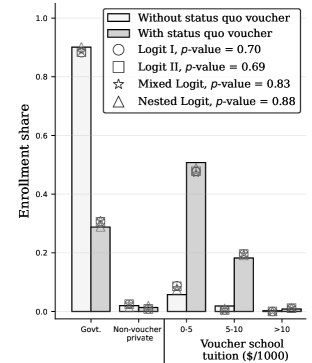
(a) Enrollment shares

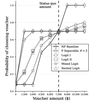
(b) Probability of voucher takeup

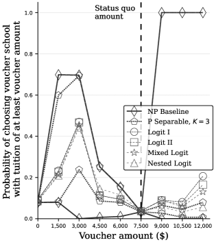
(c) Probability of takeup at schools with tuition at least voucher amount

Next, to analyze the implied demand functions at prices beyond those observed in the data, Figure 5(b)-(c) presents estimates capturing demand for the voucher in various dimensions at various counterfactual voucher amounts. In particular, Figure 5(b) presents demand for the voucher, i.e. probability of choosing $j\in\mathcal{J}_{v}$, while Figure 5(c) presents the demand for a school with tuition at least the voucher amount, i.e. probability of choosing $j\in\mathcal{J}_{v}$ such that $p^{*}_{j}\geq\tau$. In this case, comparing to the estimates under our baseline nonparametric and the reported parametric specification, we can generally observe that the demand estimates implied by the different logit models are all quite similar, and do not capture that a range of demand functions are in fact consistent with the data. Instead, they each predict unique demand functions that imply only relatively inelastic demand responses. These demand responses are towards our lower bounds, a finding which holds even when accounting for statistical uncertainty in the logit estimates as highlighted in Figure LABEL:S-fig:parameter_logit_ci. As we show below, this implies that they limit attention to only certain demand functions that can potentially drive the welfare estimates and resulting empirical conclusions.

5.3 Welfare Estimates

In Figure 6(a), we present the estimates for our various welfare parameters for the status quo voucher amount under the logit specifications as well as our baseline nonparametric and one of our parametric specifications. Moreover, in Figure 6(b), we additionally present estimates for the average surplus parameter under various counterfactual voucher amounts.

Figure 6: Welfare estimates for status quo and counterfactual amounts under various specifications

In Figure 6(a): for the nonparametric baseline and parametric separable specifications, the intervals denote the estimated lower and upper bounds; and, for the logit specifications, the markers denote the point estimates and the dashed intervals denote 90$\%$ confidence intervals computed using the percentile bootstrap with 200 draws. SOURCE: Evaluation of the DC Opportunity Scholarship Program: Final Report (NCEE 2010-4018), U.S. Department of Education, National Center for Education Statistics previously unpublished tabulations.

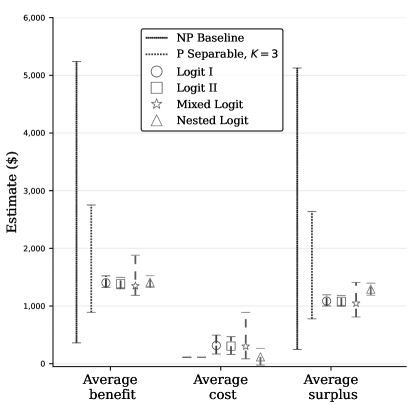
(a) Status quo amount

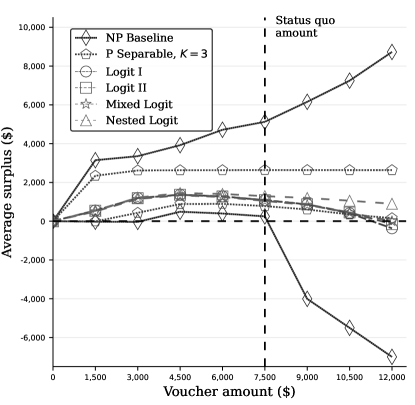
(b) $AS(\tau)$

In general, we can observe that the logit specifications all generate estimates that lie within our bounds. Intuitively, this is because the implied demand functions approximately fall in the estimated version of $\mathbf{Q}_{B}$ due to the fact they match well the data, as observed in Figure 5(a), as well as satisfy the shape restrictions in (13) as $U_{ij}$ is generally increasing given that the price coefficients are negative, as observed in Table LABEL:S-tab:logit. However, given that they limit attention to only certain demand functions as observed from Figures 5(b)-(c), they generate welfare effects that all lie within specific areas of our bounds. Relative to our estimates, this can potentially provide a misleading sense of the true effects that are consistent with the data—this also holds true when accounting for statistical uncertainty in the logit estimates as observed from the relative tight confidence intervals for the parameters in Figure 6(a) and Figure LABEL:S-fig:parameter_logit_ci.

Importantly, this can affect the interpretation of the empirical conclusions relative to those based on our estimates, previously discussed in Section 4. In particular, for voucher amounts equal to and below the status quo, our estimates can be observed to reveal positive and potentially large net benefits. In contrast, as the logit estimates all systematically fall close to our lower bounds, they can understate the potential benefits by implying only lower valuations can be consistent with the data for such voucher amounts. Alternatively, for amounts above the status quo, our estimates reveal that the data is not sufficiently rich to robustly reveal positive effects of the voucher, and caution that positive effects can be driven by only stronger assumptions. In this case, the logit estimates instead unambiguously predict positive effects and provide a false sense of robustness on the potential benefits, that are in fact driven by the parameterizations.

6 Conclusion

In this paper, we develop new discrete choice tools to robustly learn about the average willing to pay for a price subsidy and its effects on demand given exogenous, discrete variation in prices. Specifically, our tools show how to characterize what we can learn when demand is allowed to be nonparametric as well as flexibly parameterized, both of which imply that our parameters are generally partially identified. We use our tools to perform a welfare analysis of the price subsidy provided by school vouchers in the DC Opportunity Scholarship Program. We also compare our empirical results to those one would obtain under standard logit parameterizations of demand and highlight how they can provide a potentially misleading picture of the true effects.

References

- Abdulkadiroğlu et al. (2018) Abdulkadiroğlu, A., Pathak, P. A. and Walters, C. R. (2018). Free to choose: Can school choice reduce student achievement? American Economic Journal: Applied Economics, 10 175–206.
- Allende (2019) Allende, C. (2019). Competition under social interactions and the design of education policies. Job Market Paper.
- Altonji et al. (2005) Altonji, J. G., Elder, T. E. and Taber, C. R. (2005). Selection on observed and unobserved variables: Assessing the effectiveness of catholic schools. Journal of political economy, 113 151–184.
- Angrist et al. (2002) Angrist, J., Bettinger, E., Bloom, E., King, E. and Kremer, M. (2002). Vouchers for private schooling in colombia: Evidence from a randomized natural experiment. American economic review, 92 1535–1558.
- Arcidiacono et al. (2016) Arcidiacono, P., Muralidharan, K., Shim, E.-y. and Singleton, J. D. (2016). Valuing school choice: Using a randomized experiment to validate welfare evaluation of private school vouchers.
- Berry et al. (2013) Berry, S., Gandhi, A. and Haile, P. (2013). Connected substitutes and invertibility of demand. Econometrica, 81 2087–2111.
- Berry et al. (1995) Berry, S., Levinsohn, J. and Pakes, A. (1995). Automobile prices in market equilibrium. Econometrica: Journal of the Econometric Society 841–890.
- Berry and Haile (2009) Berry, S. T. and Haile, P. A. (2009). Nonparametric identification of multinomial choice demand models with heterogeneous consumers. Tech. rep., National Bureau of Economic Research.
- Berry and Haile (2014) Berry, S. T. and Haile, P. A. (2014). Identification in differentiated products markets using market level data. Econometrica, 82 1749–1797.
- Bhattacharya (2015) Bhattacharya, D. (2015). Nonparametric welfare analysis for discrete choice. Econometrica, 83 617–649.
- Bhattacharya (2018) Bhattacharya, D. (2018). Empirical welfare analysis for discrete choice: Some general results. Quantitative Economics, 9 571–615.
- Bhattacharya (2021) Bhattacharya, D. (2021). The empirical content of binary choice models. Econometrica, 89 457–474.
- Briesch et al. (2010) Briesch, R. A., Chintagunta, P. K. and Matzkin, R. L. (2010). Nonparametric discrete choice models with unobserved heterogeneity. Journal of Business & Economic Statistics, 28 291–307.
- Bugni et al. (2017) Bugni, F. A., Canay, I. A. and Shi, X. (2017). Inference for subvectors and other functions of partially identified parameters in moment inequality models. Quantitative Economics, 8 1–38.
- Carneiro et al. (2019) Carneiro, P. M., Das, J. and Reis, H. (2019). The value of private schools: Evidence from pakistan.
- Chesher et al. (2013) Chesher, A., Rosen, A. M. and Smolinski, K. (2013). An instrumental variable model of multiple discrete choice. Quantitative Economics, 4 157–196.
- Chiappori and Komunjer (2009) Chiappori, P. and Komunjer, I. (2009). On the nonparametric identification of multiple choice models.
- Compiani (2022) Compiani, G. (2022). Market counterfactuals and the specification of multiproduct demand: A nonparametric approach. Tech. Rep. 2.
- Dupas (2014) Dupas, P. (2014). Short-run subsidies and long-run adoption of new health products: Evidence from a field experiment. Econometrica, 82 197–228.
- Dynarski et al. (2018) Dynarski, M., Rui, N., Webber, A. and Gutmann, B. (2018). Evaluation of the dc opportunity scholarship program: Impacts two years after students applied. ncee 2018-4010. National Center for Education Evaluation and Regional Assistance.
- Epple et al. (2017) Epple, D., Romano, R. E. and Urquiola, M. (2017). School vouchers: A survey of the economics literature. Journal of Economic Literature, 55 441–92.
- Finkelstein et al. (2019) Finkelstein, A., Hendren, N. and Shepard, M. (2019). Subsidizing health insurance for low-income adults: Evidence from massachusetts. American Economic Review, 109 1530–67.
- Friedman (1962) Friedman, M. (1962). Capitalism and freedom. University of Chicago press.
- Gazmuri (2019) Gazmuri, A. (2019). School segregation in the presence of student sorting and cream-skimming: Evidence from a school voucher reform.
- Ho and Pakes (2014) Ho, K. and Pakes, A. (2014). Hospital choices, hospital prices, and financial incentives to physicians. American Economic Review, 104 3841–84.
- Howell et al. (2000) Howell, W. G., Wolf, P. J., Peterson, P. E. and Campbell, D. E. (2000). Test-score effects of school vouchers in dayton, ohio, new york city, and washington, dc: Evidence from randomized field trials.
- Kamat (2021) Kamat, V. (2021). Identifying the effects of a program offer with an application to head start. arXiv preprint arXiv:1711.02048.
- Kamat et al. (2022) Kamat, V., Norris, S. and Pecenco, M. (2022). Examiner designs with multiple treatments: Conviction, incarceration and policy effects. Tech. rep.
- Kitamura and Stoye (2018) Kitamura, Y. and Stoye, J. (2018). Nonparametric analysis of random utility models. Econometrica, 86 1883–1909.
- Krueger and Zhu (2004) Krueger, A. B. and Zhu, P. (2004). Another look at the new york city school voucher experiment. American Behavioral Scientist, 47 658–698.
- Levin and Driver (1997) Levin, H. M. and Driver, C. E. (1997). Cost of an educational voucher system. Education Economics, 5 265–283.
- Manski (2007) Manski, C. F. (2007). Partial identification of counterfactual choice probabilities. International Economic Review, 48 1393–1410.
- Matzkin (1993) Matzkin, R. L. (1993). Nonparametric identification and estimation of polychotomous choice models. Journal of Econometrics, 58 137–168.
- Mayer et al. (2002) Mayer, D. P., Peterson, P. E., Myers, D. E., Tuttle, C. C. and Howell, W. G. (2002). School choice in new york city after three years: An evaluation of the school choice scholarships program. final report.
- McFadden (1974) McFadden, D. (1974). Conditional logit analysis of qualitative choice behavior. Frontiers in Econometrics 105–142.
- Mills and Wolf (2017) Mills, J. N. and Wolf, P. J. (2017). Vouchers in the bayou: The effects of the louisiana scholarship program on student achievement after 2 years. Educational Evaluation and Policy Analysis, 39 464–484.
- Mogstad et al. (2018) Mogstad, M., Santos, A. and Torgovitsky, A. (2018). Using instrumental variables for inference about policy relevant treatment parameters. Econometrica, 86 1589–1619.
- Muralidharan and Sundararaman (2015) Muralidharan, K. and Sundararaman, V. (2015). The aggregate effect of school choice: Evidence from a two-stage experiment in india. The Quarterly Journal of Economics, 130 1011–1066.
- Neilson (2013) Neilson, C. (2013). Targeted vouchers, competition among schools, and the academic achievement of poor students.
- Sable and Hill (2006) Sable, J. and Hill, J. (2006). Overview of public elementary and secondary students, staff, schools, school districts, revenues, and expenditures: School year 2004-05 and fiscal year 2004. ed tab. nces 2007-309. National Center for Education Statistics.
- Tebaldi et al. (2021) Tebaldi, P., Torgovitsky, A. and Yang, H. (2021). Nonparametric estimates of demand in the california health insurance exchange. Tech. rep., National Bureau of Economic Research.
- Train (2009) Train, K. E. (2009). Discrete choice methods with simulation. Cambridge university press.
- Trivitt and Wolf (2011) Trivitt, J. R. and Wolf, P. J. (2011). School choice and the branding of catholic schools. Education Finance and Policy, 6 202–245.
- US Census (2005) US Census (2005). Public education finances.
- Wolf et al. (2010) Wolf, P., Gutmann, B., Puma, M., Kisida, B., Rizzo, L., Eissa, N., Carr, M. and Silverberg, M. (2010). Evaluation of the dc opportunity scholarship program: Final report. National Center for Education Evaluation, Institute for Education Sciences Report, 4018.