Lifetime of almost strong edge-mode operators in one dimensional, interacting, symmetry protected topological phases

Abstract

Almost strong edge-mode operators arising at the boundaries of certain interacting 1D symmetry protected topological phases with $Z_{2}$ symmetry have infinite temperature lifetimes that are non-perturbatively long in the integrability breaking terms, making them promising as bits for quantum information processing. We extract the lifetime of these edge-mode operators for small system sizes as well as in the thermodynamic limit. For the latter, a Lanczos scheme is employed to map the operator dynamics to a one dimensional tight-binding model of a single particle in Krylov space. We find this model to be that of a spatially inhomogeneous Su-Schrieffer-Heeger model with a hopping amplitude that increases away from the boundary, and a dimerization that decreases away from the boundary. We associate this dimerized or staggered structure with the existence of the almost strong mode. Thus the short time dynamics of the almost strong mode is that of the edge-mode of the Su-Schrieffer-Heeger model, while the long time dynamics involves decay due to tunneling out of that mode, followed by chaotic operator spreading. We also show that competing scattering processes can lead to interference effects that can significantly enhance the lifetime.

Topological states of matter are characterized by a bulk-boundary correspondence where non-trivial topological phases host robust edge-modes Thouless et al. (1982); Bellissard et al. (1994); Qi and Zhang (2011). While topological phases have been fully classified for free fermions Ryu et al. (2010), the stability of these phases to perturbations such as non-zero temperature, disorder, and interactions, is poorly understood. The expectation is that as long as the perturbations are smaller than the bulk single-particle energy gap, the edge-modes will survive. More surprisingly, examples are beginning to emerge where even at high temperatures of the order of the band width, and with moderate interactions, the edge-modes while not completely stable, have extremely long lifetimes Kemp et al. (2017); Else et al. (2017); Kemp et al. (2019); Rakovszky et al. (2020). Since edge-modes can be used as qubits, understanding these non-perturbatively long lifetimes is of fundamental importance both for theory and for applications.

We study a class of 1D models that in the limit of free fermions correspond to Class-D in the Altland-Zirnbauer classification scheme Ryu et al. (2010); Altland and Zirnbauer (1997). These models host Majorana modes, and are promising candidates for non-Abelian quantum computing Kitaev (2001, 2006); Fidkowski and Kitaev (2011); Nayak et al. (2008); Fendley et al. (2009); Alicea (2012); Beenakker (2013). Adding interactions and raising the temperature do not appear to destabilize the edge-modes easily Kemp et al. (2017); Else et al. (2017); Parker et al. (2019a); Kemp et al. (2019); Vasiloiu et al. (2018). Similar behavior has been found in interacting, disorder-free, Floquet systems where bulk quantities heat to infinite temperature rapidly, i.e., within a few drive cycles, and yet edge-modes coexist with the high temperature bulk for an unusually long time Yates et al. (2019). A hurdle to understanding these lifetimes is that they are extracted from exact-diagonalization (ED), and this is plagued by system size effects making it difficult to extract lifetimes in the thermodynamic limit.

We present a fundamentally new scheme to extract the long lifetimes of topological edge-modes. Using a Lanczos scheme, we map the Heisenberg time-evolution of the edge-mode operator onto a Krylov basis where the dynamics is equivalent to a single-particle on a tight-binding lattice with inhomogeneous couplings Vishwanath and Müller (2008); Parker et al. (2019b); Barbón et al. (2019). We find that this lattice for the edge-mode operators is neither that of an operator of a free or integrable model, nor is it the lattice typical of a chaotic operator. We give arguments for the general structure of the Krylov lattice of these topological edge-modes, and analytically extract the lifetime.

Model: We study the anisotropic $XY$ model of chain length $L$, perturbed by a transverse field, and by exchange interactions in the $z$ direction,

$$H =\sum_{i=1}^{L}\biggl{[}J\left(\frac{1+\gamma}{2}\right)\sigma_{i}^{x}\sigma_{i+1}^{x}+J\left(\frac{1-\gamma}{2}\right)\sigma_{i}^{y}\sigma_{i+1}^{y}$$

$$+J_{z}\sigma_{i}^{z}\sigma_{i+1}^{z}+g\sigma_{i}^{z}\biggr{]}=H_{\rm XX}+H_{\rm YY}+H_{\rm ZZ}+H_{Z},$$ (1)

where $g$ and $\gamma$ denote the strength of the transverse field and the $XY$ anisotropy respectively. We set $J=\hbar=1$. A non-zero $J_{z}$ prevents a mapping to free Jordan-Wigner fermions. The model has a $Z_{2}$ symmetry $D_{z}=\sigma_{1}^{z}\sigma_{2}^{z}\dots\sigma_{L}^{z}$. For $\gamma\neq 0,J_{z}=0,|g|<1$, or $\gamma\neq 0,J_{z}\neq 0,g=0$, the model supports a strong mode (SM) operator defined as Kitaev (2001); Fendley (2012); Jermyn et al. (2014); Fendley (2016); Maceira and Mila (2018)

$$\{\Psi_{0},D_{z}\}=0,\qquad[H,\Psi_{0}]\approx u^{L};\;\;||u||<1.$$ (2)

Thus, as $L\rightarrow\infty$, $\left[H,\Psi_{0}\right]=0$. Existence of a SM implies that the two different parity sectors are degenerate as $L\rightarrow\infty$ Moran et al. (2017); Vasiloiu et al. (2019).

When $J_{z}\neq 0$, the SM turns into an almost strong mode (ASM) Kemp et al. (2017) that anti-commutes with parity, but only approximately commutes with $H$ when $L\rightarrow\infty$. While for small system sizes, the ASM behaves similarly to the SM as it’s lifetime increases exponentially with $L$, for larger $L$ however, its lifetime saturates to a system-size independent value.

SM for $J_{z}=0$: While the SM is $\Psi_{0}=\sigma^{x}_{1}$ when $J_{z}=g=0,\gamma=1$, for other parameters, it is a more complicated operator which nevertheless has a finite overlap with $\sigma^{x}_{1}$. In terms of Majorana fermions defined as:

$$a_{2l-1}=\sigma^{x}_{l}\prod_{j=1}^{l-1}\sigma^{z}_{j},\;\;a_{2l}=\sigma^{y}_{l}\prod_{j=1}^{l-1}\sigma^{z}_{j},\,$$ (3)

and for $\gamma>0$, we find that the SM localized at one end is Sup

$$\Psi_{0}=\sum_{l=1}^{L-1}C_{l}a_{2l-1};\;\;C_{l}=\frac{(1+\gamma)/2}{\sqrt{g^{2}+\gamma^{2}-1}}\Big{(}q_{+}^{l}-q_{-}^{l}\Big{)},$$

$$q_{\pm}=\frac{g\pm\sqrt{g^{2}+\gamma^{2}-1}}{1+\gamma}.$$ (4)

$\Psi_{0}$ is normalizable for $g^{2}<1$, $\gamma\neq 0$, indicating that it is localized at the boundary. When $\gamma=1$, the SM is the familiar one for the Kitaev chain with Kitaev (2001) $C_{l}=g^{l-1}$. that, just like the correlations Franchini and Abanov (2005), the spatial character of the SM changes at $g^{2}+\gamma^{2}=1$. from over-damped to under-damped decay where in the $g^{2}+\gamma^{2}<1$, we have decay of the SM does not depend

Autocorrelation function: Due to the overlap with $\sigma^{x}_{1}$ when $\gamma>0$, the SM and ASM (together denoted by (A)SM) might be detected through the infinite temperature auto-correlation function Kemp et al. (2017) defined as,

$$A_{\infty}(t)=\frac{1}{2^{L}}\text{tr}\left[\sigma_{1}^{x}(t)\sigma_{1}^{x}(0)\right].$$ (5)

Here $\hat{O}(t)=e^{iHt}\hat{O}e^{-iHt}$ denotes Heisenberg time-evolution. In general, $A_{\infty}(t)\sim e^{-\Gamma t}$ decays in time. For a finite wire the (A)SM can tunnel across, and the decay-rate is exponentially dependent on $L$ as suggested in Eq. (2), with $\Gamma\sim e^{-Lh(\gamma,g,J_{z})}$ for some function $h$, to be determined. The exponential increase in lifetime with system size is a characteristic of the SM. In contrast, for the ASM, the exponential increase of lifetime with system size eventually saturates to a $L$ independent result. For example, when $\gamma=1$, ED suggests a highly non-perturbative dependence $\Gamma\sim e^{-cJ/J_{z}},c=O(1)$ upto logarithmic corrections Else et al. (2017). This form is also argued from setting operator bounds on approximately conserved quantities in the prethermal regime Abanin et al. (2017). However a treatment that directly studies lifetime of topological edge-modes, and is valid for broader regimes, not necessarily related to prethermalization, is needed.

Figure 1: Decay-rate of $A_{\infty}$ obtained from ED for different $L$ and $J_{z}$, behaves as $\Gamma=\left({\rm max}(J_{z},J_{y})\right)^{L/2}$, where $g\ll J_{z,y}\ll 1$. When $J_{z}=J_{y}$, destructive interference between two scattering channels leads to leads to a pronounced increase of the lifetime as indicated by the cusp.

Lifetime for small system sizes: We now show that the lifetime for small system sizes is largely governed by perturbative processes. Denoting $|\epsilon_{n}\rangle$ as an eigenstate of $H$ and parity, even in the presence of integrability breaking terms, $\sigma_{1}^{x}|\epsilon_{n}\rangle\sim|\epsilon_{n}^{\prime}\rangle$, where $\epsilon_{n}^{\prime}$ is the opposite parity energy level nearly degenerate to $\epsilon_{n}$. Defining $\Delta_{n}=\epsilon_{n}-\epsilon_{n}^{\prime}$, we find that to a good approximation the finite-size behavior is mimicked by Sup $A_{\infty}(t)\sim\sum_{n}\cos(\Delta_{n}t)/2^{L-1}$. For the finite-size decay-rate, a perturbative estimate of $\Delta_{n}$ suffices. Below we treat $J_{y,z},g\ll 1$, where $J_{y}=(1-\gamma)/2$. Focusing on the two degenerate ground states of $H_{\rm XX}$ (not necessarily of definite parity) we determine the process that gaps the states, and from that construct the two gapped states of definite parity. The same considerations hold for every excited level of $H_{\rm XX}$.

Denoting the eigenstate of $\sigma^{x}$ as, $\sigma^{x}|\pm\rangle=\pm|\pm\rangle$, let us first consider the case when $g$ is dominant. $L$ applications of $g$ are required for a transition from one ground state to another, $|++\dots+\rangle\xrightarrow{(g\sum_{i}\sigma_{i}^{z})^{L}}|--\dots-\rangle$. Thus the splitting between the ground state sectors is $g^{L}$, and the same splitting appears when rotated to the basis of definite parity, $|++\dots+\rangle\pm|--\dots-\rangle$. The energy splitting gives a decay rate of the ASM, $\Gamma\sim g^{L}=e^{\log(g)L}$.

When $J_{z}$ is the dominant term, the ground state degeneracy is lifted by $L/2$ applications of $J_{z}$, $|++\dots+\rangle\xrightarrow{(J_{z}\sum_{i}\sigma_{i}^{z}\sigma_{i+1}^{z})^{L/2}}|--\dots-\rangle$, giving an energy splitting and consequently a decay-rate $\Gamma\sim(J_{z})^{L/2}=e^{\log(J_{z})L/2}$. Similar arguments can be applied when $J_{y}$ is dominant. Since, $\sigma_{i}^{y}\sigma_{i+1}^{y}=-\sigma_{i}^{x}\sigma_{i+1}^{x}\sigma_{i}^{z}\sigma_{i+1}^{z}$, up to an overall sign, $J_{y}$ is similar to the $J_{z}$ perturbation and gives, $\Gamma\sim(J_{y})^{L/2}=e^{\log(J_{y})L/2}$. Fig. 1 plots $\Gamma$ obtained from ED. The solid lines are the estimates for $\Gamma$ from perturbation theory, and they excellently describe the asymptotic behavior of the data. In addition, the plot shows an interesting phenomenon when competing terms affect the lifetime. In particular, when $J_{y}\sim J_{z}$, since matrix elements of the two terms have opposite signs, destructive interference between these two scattering channels leads to an enhanced lifetime. This is visible as a pronounced cusp in Fig. 1 when $J_{y}\sim J_{z}$.

Krylov basis: We now discuss the lifetime of the ASM in the system-size independent limit. We study the operator dynamics following a Lanczos scheme designed to map the Heisenberg time-evolution to a tight-binding model in Krylov space Vishwanath and Müller (2008); Parker et al. (2019b). Note that, $\sigma_{1}^{x}(t)=e^{iHt}\sigma_{1}^{x}e^{-iHt}=\sum_{n=0}^{\infty}\frac{\left(it\right)^{n}}{n!}\mathcal{L}^{n}\sigma_{1}^{x}$, where $\mathcal{L}=\left[H,\cdot\right]$. We define $\hat{O}=|O)$, and $(O_{1}|O_{2})=\frac{1}{2^{L}}\text{tr}\left[O_{1}^{\dagger}O_{2}\right]$. Thus $A_{\infty}(t)$ becomes,

$$A_{\infty}(t)=(\sigma_{1}^{x}|e^{it\mathcal{L}}|\sigma_{1}^{x}).$$ (6)

The Pauli basis is $2^{2L}$ dimensional, hence determining $\mathcal{L}$ outright is generally not feasible. $\sigma_{1}^{x}$ is a Majorana, and when the system is free, the time evolution can only mix with a total of $2L$ Majoranas, and only in this case can $\mathcal{L}$ be completely determined. However, the key observation is that for both free and interacting cases, there is a special basis, the Krylov basis, where $\mathcal{L}$ is tri-diagonal, and the dynamics of any operator can be mapped to a tight-binding model.

To construct the Krylov basis for say $\sigma^{x}_{1}$, we start with $|O_{0})=|\sigma_{1}^{x})$, and construct $|A_{1})=\mathcal{L}|O_{0})$, $b_{1}=\sqrt{(A_{1}|A_{1})}$, and $|O_{1})=|A_{1})/b_{1}$. These steps are repeated as follows,

$$|A_{n})=\mathcal{L}|O_{n-1})-b_{n-1}|O_{n-2}),$$

$$b_{n}=\sqrt{(A_{n}|A_{n})};|O_{n})=\frac{1}{b_{n}}|A_{n}).$$ (7)

In the Krylov basis, the Liouvillian takes the form,

$$\mathcal{L}=H_{K}=\sum_{i}b_{i}\left(c_{i}^{\dagger}c_{i+1}+h.c.\right),$$ (8)

where $c_{i}^{\dagger},c_{i}$ are the creation, annihilation operators in the Krylov basis. Recently, this approach has been mainly used to identify chaos Parker et al. (2019b); Barbón et al. (2019); Dymarsky and Gorsky (2019). Below we show that this method is very helpful for studying long-lived topological edge-modes.

Lifetime in the thermodynamic limit: The (A)SM can be constructed by noticing that

$$[H_{K},c_{1}^{\dagger}]=b_{1}c_{2}^{\dagger},\;\;\;[H_{K},c_{1}^{\dagger}-\frac{b_{1}}{b_{2}}c_{3}^{\dagger}]=-\frac{b_{1}b_{3}}{b_{2}}c_{4}^{\dagger},$$

$$[H_{K},c_{1}^{\dagger}-\frac{b_{1}}{b_{2}}c_{3}^{\dagger}+\frac{b_{1}b_{3}}{b_{2}b_{4}}c_{5}^{\dagger}]=\frac{b_{1}b_{3}b_{5}}{b_{2}b_{4}}c_{6}^{\dagger}\dots.$$ (9)

Thus the ASM after $N$ iterations is,

$$\Psi_{0}(N)=\sum_{n=0}^{N}(-1)^{n}\frac{b_{1}b_{3}\dots b_{2n-1}}{b_{2}b_{4}\dots b_{2n}}c_{2n+1}^{\dagger}.$$ (10)

The error, defined by how much $\Psi_{0}(N)$ does not commute with $H_{K}$ is

$$\!\!\text{error}(N)=[H,\Psi_{0}(N)]\!\!=(-1)^{N}\frac{b_{1}\dots b_{2N-1}b_{2N+1}}{b_{2}\dots b_{2N}}c_{2N+2}^{\dagger}.$$ (11)

The error is an important quantity for identifying an (A)SM. This is because for a SM, the error only decreases with subsequent iterations, whereas for an ASM, the error decreases up to a certain $N^{*}$, and then begins to grow. In addition, as we show below, the error at $N^{*}$ can be used to determine the lifetime in the thermodynamic limit.

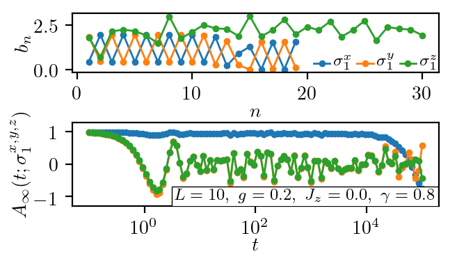
Figure 2: Top panel: The $b_{n}$ for the Pauli spins on the first site $\sigma_{1}^{x,y,z}$ for $J_{z}=0,\gamma>0$. The model maps to free fermions and supports a SM with overlap with $\sigma^{x}_{1}$. The deviation from perfect staggered behavior for $n>10$ is a finite-size effect. Bottom panel: $A_{\infty}$ from ED for $\sigma^{x,y,z}_{1}$. Due to overlap with the SM, $\sigma^{x}_{1}$ persists up to $t\sim 10^{4}$ as opposed to $\sigma^{y,z}_{1}$ that decay by $t=O(1)$.

First consider $J_{z}=0,g^{2}<1$, for which a SM exists (c.f. Eq. (4)). We find that the Krylov Hamiltonian for $\sigma^{x}_{1}$ with $\gamma=1$ is, $b_{\rm odd}=2g,b_{\rm even}=2$, and therefore has a staggered/dimerized structure quantified by $b_{2n}-b_{2n+1}>0$. For $\gamma\neq 1$, the $b_{n}$ are shown in Fig. 2, and show a similar staggered structure. Thus the effective Hamiltonian in the Krylov basis is the Su-Schrieffer-Heeger (SSH) model Su et al. (1979, 1980), with the SM being the edge-mode of the SSH model. For the same parameters, other Pauli operators such as $\sigma^{y,z}_{1}$ which are not localized at the edge under Heisenberg time-evolution, have a qualitatively different Krylov Hamiltonian. In particular, $\sigma^{y}_{1}$ is given by an SSH-type model but with a dimerization of the opposite sign to that of $\sigma^{x}_{1}$, so that the effective Hamiltonian for $\sigma^{y}_{1}$ is topologically trivial and supports no localized edge-mode. Since topological protection is robust to moderate disorder, local fluctuations of the above staggered structure in Krylov space will not affect the stability of the edge-mode. The pattern of staggering of $b_{n}$ in Fig. 2 continues until $n\sim O(L)$, after which finite-size effects, such as the hybridization of the Majoranas at the ends of the chain, set in.

The Krylov basis for $\sigma^{z}_{1}$ is different from $\sigma^{x,y}_{1}$ in that to start with, near site $1$ the dimerization is negative, corresponding to a topologically trivial phase. But on moving towards the bulk, the average hopping first increases, and then plateaus. The net effect on the dynamics is similar to that on $\sigma^{y}_{1}$ in that this lattice causes the operator to spread rapidly into the bulk under time-evolution. The lower panel of Fig. 2 shows the $A_{\infty}$ of the 3 Pauli operators, with $\sigma^{y,z}_{1}$ decaying rapidly.

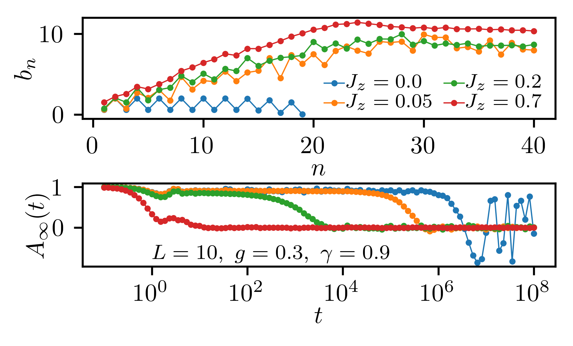
Figure 3: Top panel: The $b_{n}$ for increasing $J_{z}$ with finite-size effects appearing as a plateau for $n>20$. As $L$ is increased Sup , the linear ramp is extended, with the $b_{n}$ plateauing at a larger $n$ and at a larger value. Bottom panel: $A_{\infty}$ shows rapid decrease in lifetime with increasing $J_{z}$.

Fig. 3, top panel shows how the $b_{n}$ change on increasing $J_{z}$. The corresponding $A_{\infty}$ is plotted in the lower panel of Fig. 3. One finds that the effect of $J_{z}$ is two-fold, one is to increase the average hopping into the bulk, which appears as a non-zero slope of $b_{n}$ when plotted against $n$. The second effect is to reduce the dimerization with increasing $n$. Eventually, deep in the bulk, the dimerization vanishes, and the effective hopping increases linearly with position, a behavior expected for a generic chaotic operator Parker et al. (2019b); Barbón et al. (2019). The long lifetime of the ASM is entirely due to this crossover from the topologically non-trivial SSH model at small $n$, to chaotic linear couplings at large $n$.

Effective model in Krylov basis: We make this more quantitative by adopting the following model for the hopping parameters

$$b_{2n} =\alpha_{0}+\rho\alpha 2n+\delta;\quad 0<\alpha\ll\alpha_{0}\sim\delta;$$

$$b_{2n+1} =\alpha_{0}+\alpha(2n+1);\quad 0<1-\rho\ll 1\,.$$ (12)

The even sites have slope $\rho\alpha$, while the odd sites have slope $\alpha$. At some point the dimerization $b_{2n}-b_{2n+1}$ changes sign as $\rho<1$. This means that Eq. (11) eventually grows with $N$ and the mode is non-normalizable. We also imposed $1-\rho<<1$ to simplify analytic expressions but this restriction is not essential.

We can estimate the decay-rate from Eq. (11) by finding $N^{*}$ such that $b_{2N^{*}+1}=b_{2N^{*}}$ which gives, $N^{*}\sim\delta/2\alpha(1-\rho)\gg 1$ and,

$$\Gamma\sim|\text{error}(N^{*})|=b_{1}\exp\left[\sum_{n=1}^{N^{*}}\ln\biggl{(}\frac{b_{2n+1}}{b_{2n}}\biggr{)}\right]$$

$$\sim\exp\left[-\frac{\delta}{2\alpha}\log\left(\frac{1}{1-\rho}\right)\right].$$ (13)

Note that when $\rho=1,\alpha\neq 0$, we still have a SM despite the fact that the $b_{n}$ have a linear slope $b_{n}\sim\alpha n$. Thus it is the dimerization, which is preserved when $\rho=1$, that prevents the operator from spreading. Eq. (13) shows that the lifetime depends on $J_{z}$ non-perturbatively as the slope $\alpha\propto J_{z}$. We later give numerical and qualitative arguments for this form of the slope.

It is illuminating to consider the continuum limit of the effective Hamiltonian in the Krylov basis, where the the eigenvalue problem may be recast as Sup , $E\Psi_{n}=\biggl{[}\left(b_{2n-1}-b_{2n}-b_{2n}\partial_{n}\right)\sigma^{-}+h.c\biggr{]}\Psi_{n}$. The edge-mode solution is,

$$\Psi_{0,n}=e^{-\int^{n}_{1}dm\frac{b_{2m}-b_{2m-1}}{b_{2m}}}\begin{pmatrix}1\\ 0\end{pmatrix},$$ (14)

and shows that the ASM, indeed, decreases in amplitude into the bulk when $(b_{2m}-b_{2m-1})/b_{2m}>0$. Using the minimal model in Eq. (12), we see that at $N^{*}$, $b_{2N^{*}}-b_{2N^{*}+1}=0$,  (14) stops decreasing with $n$ and mixes with other modes. The decay-rate is estimated by the value of ASM at $n=N^{*}$, $\Gamma\sim\exp\left[-\int^{N^{*}}dm\frac{b_{2m}-b_{2m-1}}{b_{2m}}\right]$ which recovers Eq. (13).

Comparison of ED with Krylov Hamiltonian with a metallic bulk: We extract the non-perturbative lifetime using two different numerical methods. Top panel of Fig. 4 compares $A_{\infty}$ from ED for $L=14$, to that obtained from time-evolving by the Krylov Hamiltonian $\langle n=1|\left[\exp\left(iH_{K}t\right)\right]|n=1\rangle$, where $|n=1\rangle$ is a state localized at site 1 in the Krylov basis. Since the calculation of the $b_{n}$ is exponentially expensive in computer resources, only the first $\sim 40$ $b_{n}$ are evaluated. Guided by Fig. 3, we simulate a semi-infinite lattice in Krylov space by setting $b_{40<n<2e5}=b_{40}$, essentially attaching a metallic reservoir to our inhomogeneous SSH model. The lifetime obtained by both these methods is shown in the lower panel of Fig. 4, and suggests the $L$ independent form $\ln\Gamma\propto-1/J_{z}$. Thus for the purpose of capturing the lifetime, the simple model for the bulk $b_{n}$ is an efficient alternative to ED. In addition, the saturation of the lifetime implies that it is controlled by the dimerization of the $b_{n}$ at small and intermediate $n$. Sup

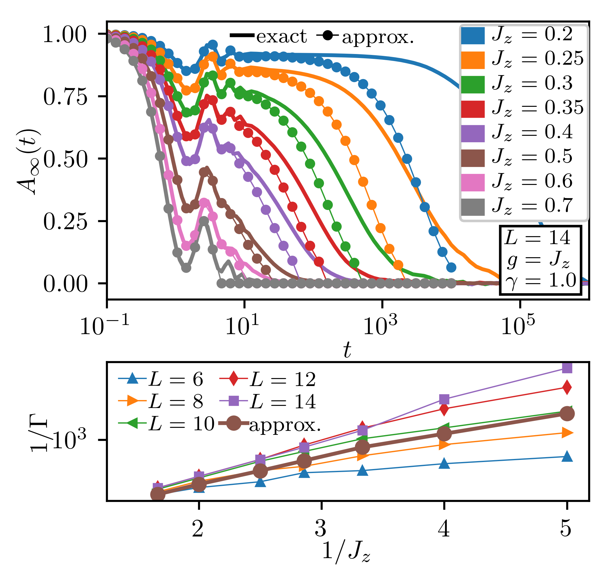
Figure 4: Top panel: $A_{\infty}$ from ED for $L=14$, with $J_{z}=g$ increasing from the top to the bottom of the panel. It is compared with the approximate $A_{\infty}$ obtained from time-evolution in a Krylov basis with $\sim 40$ exact $b_{n}$ Sup , and $b_{40<n<n_{\rm max}}=b_{40}$ held constant, mimicking a reservoir. We choose $n_{\rm max}=2e5$, which is large enough to capture the decay of the ASM before finite-size effects set in. Bottom panel: Decay-rate extracted from both numerical methods. For $1/J_{z}<4$, the overlapping lines for $L=12,14$ indicates saturation of the lifetime.

Qualitative argument for $\alpha\propto J_{z}$: We supplement the above results for the decay-rate by a qualitative argument for $\alpha\propto J_{z}$. For simplicity we restore $J$ and consider $\gamma=1$. When $J_{z}=g=0$, then $H=H_{\rm XX}=JN$ counts the number of domain walls $N=\sum_{i}\sigma^{x}_{i}\sigma^{x}_{i+1}$. When $J_{z}\neq 0$ we recast $H_{ZZ}=J_{z}D+J_{z}\tilde{E}$, where $D$ commutes with $N$, whereas $\tilde{E}$ does not. We find that the operator,

$$D=\sum_{j}P_{j}\sigma^{z}_{j}\sigma^{z}_{j+1};\;\;P_{j}=\frac{1}{2}\biggl{[}1-\sigma^{x}_{j-1}\sigma^{x}_{j}\sigma^{x}_{j+1}\sigma^{x}_{j+2}\biggr{]},$$ (15)

does not change the number of domain walls and commutes with $N$Sup . $D$ is essentially a hopping term for domain walls. In the basis that simultaneously diagonalizes $D,N$ we find that the minimal energy to create a domain wall in the bulk is reduced from $2J$ to $2J-J_{z}$, and that domain wall particle-hole pairs have energies of O($J_{z}$). Now consider $J_{z}\ll g$. Then the leading term non-commuting with $N$ is $H_{Z}$.

As argued for a different model Kemp et al. (2019), the energy cost for flipping a spin at the edge is $\sim J$. Thus a creation of $\sim J/J_{z}$ pairs of domain walls in the bulk can off-set the energy $J$ required to flip an edge spin. This requires $J/J_{z}$ applications of the transverse field $g$. Therefore the Fermi-Golden rule estimate for the decay rate is,

$$\Gamma\sim g\biggl{[}\frac{g}{J}\biggr{]}^{cJ/J_{z}},\;\;\;c=O(1).$$ (16)

Upto logarithms, this decay-rate is consistent with ED Else et al. (2017) (Fig. 4), operator bounds in the prethermal regime Abanin et al. (2017), and with time-evolution using a truncated Krylov Hamiltonian (Fig. 4).

Summary: We have presented a new way to extract the non-perturbatively long lifetimes of ASMs. We showed that the Krylov Hamiltonian for the ASM has linearly growing hopping along with decreasing dimerization, where the dimerization is associated with the existence of the ASM and is key to preventing chaotic operator growth. Essentially the operator dynamics is that of a particle which is trapped for a long time as a quasi-stable SSH edge-mode that eventually escapes via tunneling. We demonstrated that a truncated Krylov Hamiltonian terminating in a metallic bulk is an efficient way for capturing the lifetime of the ASM. We also found that competing terms can interfere to enhance the lifetime (Fig. 1). It would be interesting to identify additional structures of the Krylov Hamiltonian, besides dimerization, that can support long-lived edge-modes. More broadly, generalization of this study to other topological states, both static and Floquet, and in any spatial dimension, is an exciting avenue for future research.

Acknowledgements: This work was supported by the US Department of Energy, Office of Science, Basic Energy Sciences, under Award No. DE-SC0010821 (DJY and AM) and by the US National Science Foundation Grant NSF DMR-1606591 (AGA).

Supplementary Material: Lifetime of almost strong edge mode operators in one dimensional, interacting, symmetry protected topological phases

The supplementary material contains:
1. Three supplementary plots.
2. Derivation of SM for general $\gamma$.
3. Derivation of the continuum model.
4. Derivation of Eq. (16).

Figures showing the autocorrelation function of $\sigma^{x}_{1}$ and also the effective Krylov hoppings

In this section we present three additional plots for the autocorrelation function, and for the $b_{n}$ parameters of the Krylov Hamiltonian.

The existence of the (almost) strong mode (A)SM leads to the near degeneracy of energy levels of opposite parity. Let us denote $|\epsilon_{n}\rangle$ as an eigenstate of $H$ and parity. Then, even in the presence of integrability breaking terms, $\sigma_{1}^{x}|\epsilon_{n}\rangle\sim|\epsilon_{n}^{\prime}\rangle$, where $\epsilon_{n}^{\prime}$ is the opposite parity energy level nearly degenerate to $\epsilon_{n}$. Defining $\Delta_{n}=\epsilon_{n}-\epsilon_{n}^{\prime}$, we find that to a good approximation the finite-size behavior is mimicked by

$$A_{\infty}(t)\sim\sum_{n}\cos(\Delta_{n}t)/2^{L-1}\,.$$ (17)

Fig. 5 shows the exact autocorrelation function obtained from ED and compares it with the approximation (17) computed for $\Delta_{n}=\epsilon_{n}-\epsilon_{n}^{\prime}$ where the level $\epsilon_{n}^{\prime}\equiv\epsilon_{m}$ is found with the following relation, $\text{argmax}_{m}|\langle m|\sigma_{1}^{x}|n\rangle|^{2}$. One can see that this approximation reproduces the lifetime not only for small system sizes, but also for larger systems where the lifetime has saturated (ie, become $L$ independent).

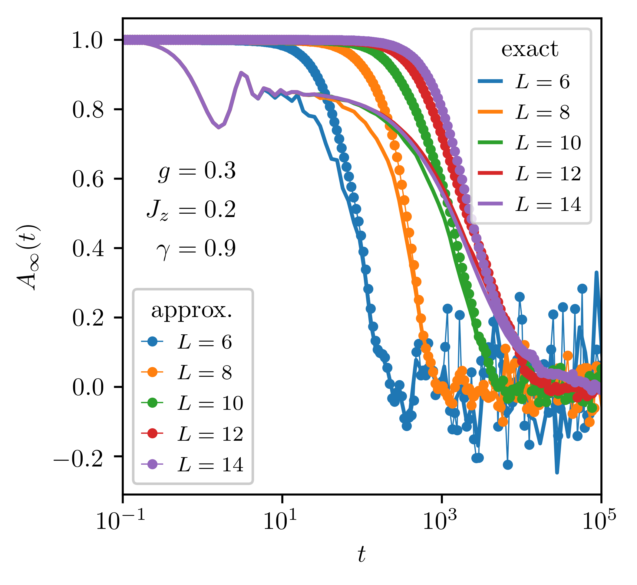
Figure 5: Exact autocorrelation function obtained from ED and compared with the approximation $A_{\infty}(t)\sim A_{\infty}^{C}(t)=\sum_{n}\cos(\Delta_{n}t)/2^{L-1}$. If for nearly all eigenstates $|n\rangle$, there exists another eigenstate state $|m(n)\rangle$, such that, $|\langle m(n)|\sigma_{1}^{x}|n\rangle|^{2}\sim 1$, then $A^{C}_{\infty}$ is a good approximation, and estimates the lifetime well. In fact it reproduces the lifetime before system size saturation, as well as the system size independent results.

Fig. 6 shows the $b_{n}$ for different $J_{z}$ and for different system sizes. It also shows the corresponding $A_{\infty}(t)$ from ED for the same parameters. The figure suggests that for chains exhibiting an anomalously long lifetime in the autocorrelation function, the Krylov parameters $b_{n}$ have three main features, a ramp upwards at small $n$, a system-size dependent plateau at intermediate and large $n$, and $J_{z},g,\gamma,n$ dependent staggering or dimerization of the $b_{n}$.

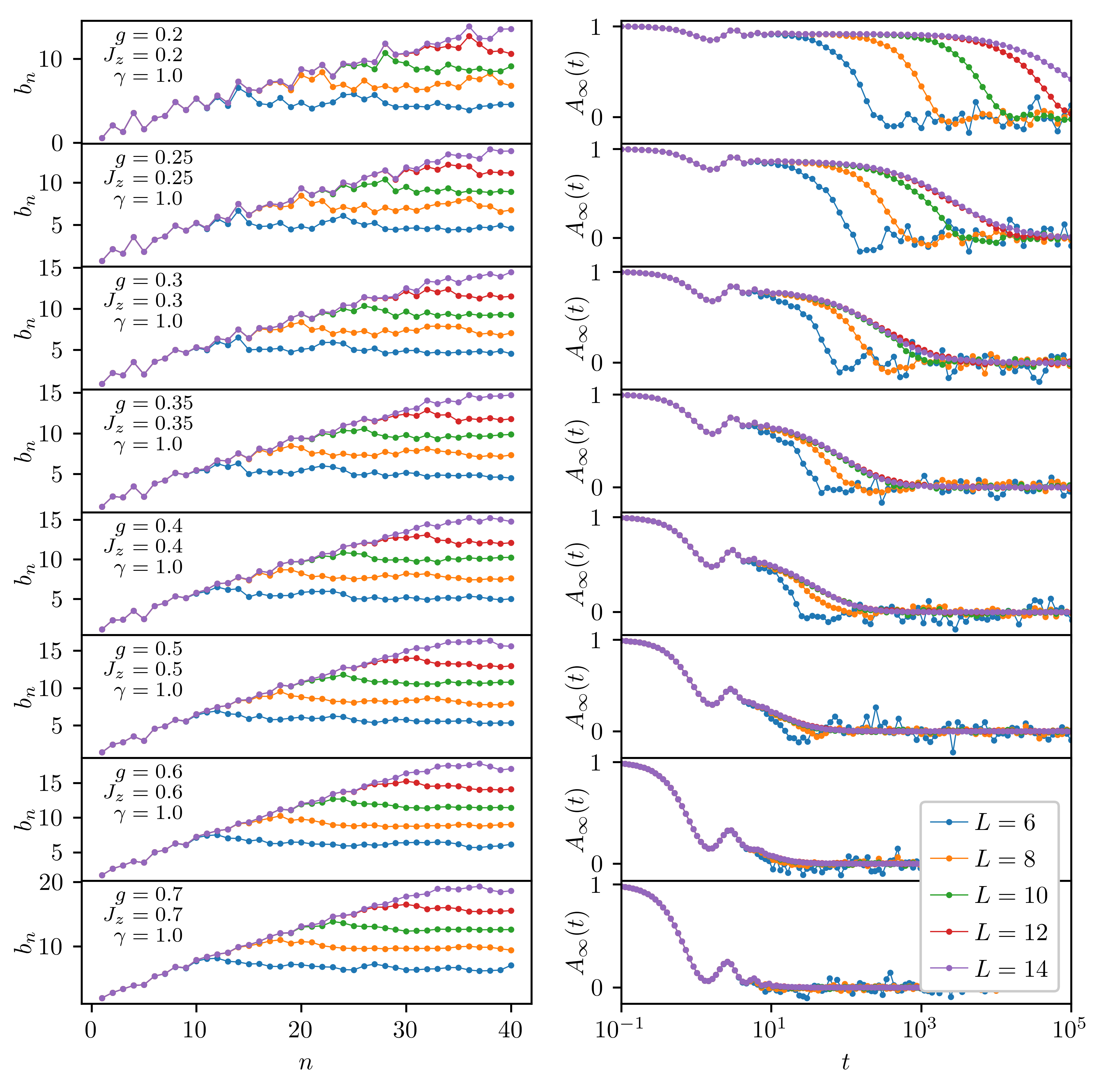
Figure 6: Left column, $b_{n}$ for different $J_{z}$ and for different system sizes. We also take $g=J_{z}$ as in Fig. 4 in the main text. Right column, $A_{\infty}(t)$ from ED for the same parameters as the left column. All $A_{\infty}(t)$ show saturation in system size for $J_{z}\geq 0.25$. The $b_{n}$ have three main features, a ramp upwards at small $n$, a system-size dependent plateau at intermediate and large $n$, and $J_{z},g,\gamma,n$ dependent staggering or dimerization of the $b_{n}$. The Krylov subspace of $\sigma_{1}^{x}$ is $\propto 2^{2L}$ and generally, the plateaus in the the left column extend out to very large $n$. As the $b_{n}$ are exponentially difficult to compute, only the first 40 are shown. Knowledge of all $b_{n}$ and usage of Eq. (6) will reconstruct the right column exactly. From top to bottom, both sides, $J_{z}$ is increased. The increase in $J_{z}$ drastically reduces the lifetime of $A_{\infty}(t)$ while simultaneously diminishing the staggering of the $b_{n}$. In particular, the onset of a “smooth” $b_{n}$ structure is moved to smaller $n$ as one increases $J_{z}$.

Fig. 7 shows how $b_{n}$ varies for different $J_{z}$, for system size $L=14$. The overall staggering in $b_{n}$ is reduced as one increases $J_{z}$, and the staggering is also stronger at smaller $n$. We associate this staggered structure at small $n$ with the existence of the ASM.

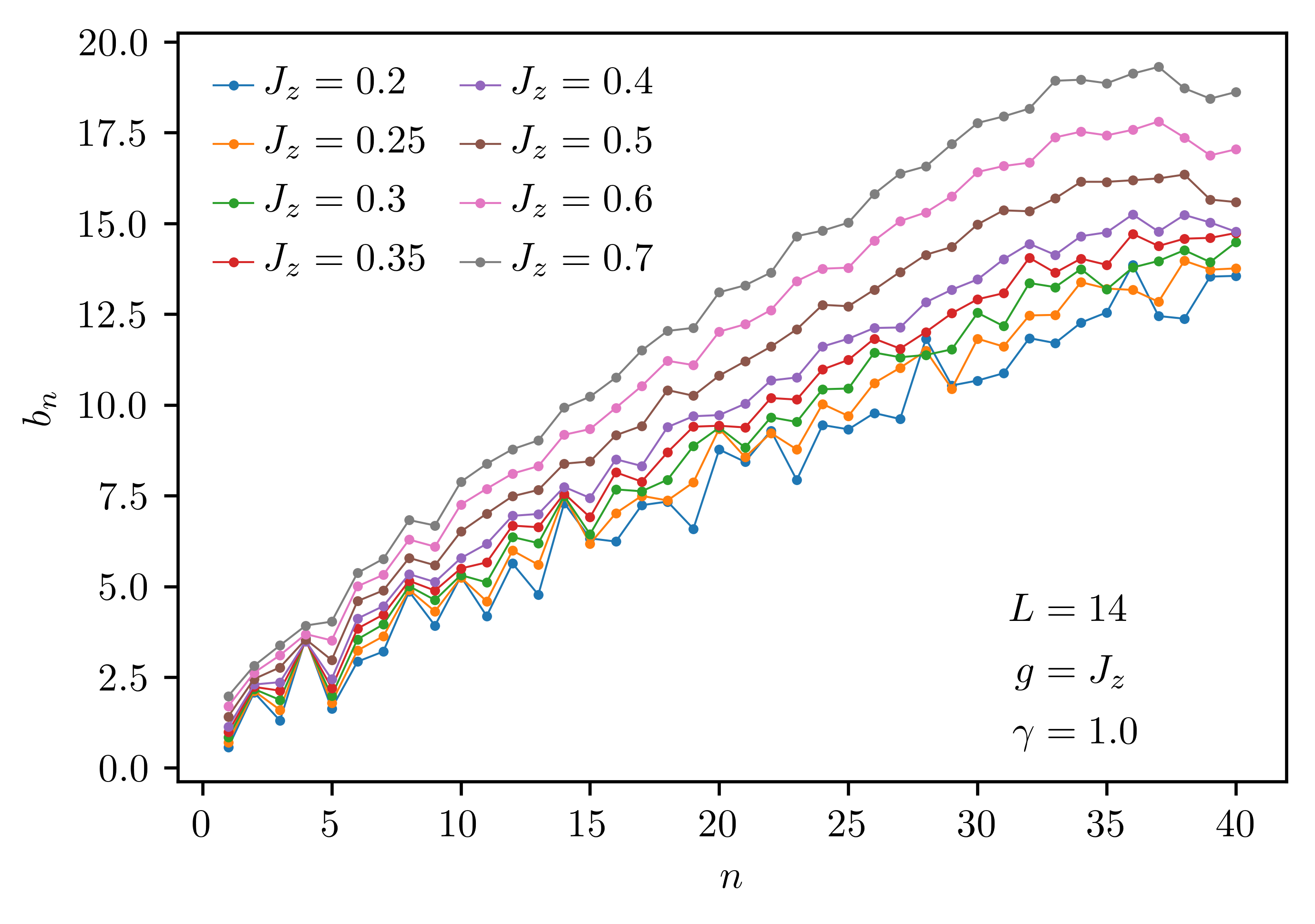
Figure 7: The $b_{n}$ for different $J_{z}$ for system size $L=14$ shown in Fig. 6. Overall staggering in $b_{n}$ is reduced as one increases $J_{z}$, and the staggering is also stronger at smaller $n$. The approximate $A_{\infty}$ shown in Fig. 4 in main text is constructed from these $b_{n}$ followed by an approximate “plateau” of $b_{n>40}=b_{40}$ for $n$ from 41 to 200,041.

Constructing zero-mode for the $XY$ model $J_{z}=0$

For $J_{z}=0$ the model (1) in the main text can be reduced to a model of non-interacting Majorana fermions. Defining,

$$a_{2l-1}=\sigma^{x}_{l}\prod_{j=1}^{l-1}\sigma^{z}_{j},\qquad a_{2l}=\sigma^{y}_{l}\prod_{j=1}^{l-1}\sigma^{z}_{j},$$ (18)

we obtain from (1) in main text

$$H=i\sum_{l=1}^{L}\left[-\frac{1+\gamma}{2}a_{2l}a_{2l+1}+\frac{1-\gamma}{2}a_{2l-1}a_{2l+2}-ga_{2l-1}a_{2l}\right]\,.$$ (19)

Here one should assume $a_{2L+1}=a_{2L+2}=0$, as this ensures that $\sigma^{x,y}_{L+1}$ is outside the system. It is straightforward to construct the operators $\Psi_{k}$ such that $\left[H,\Psi_{k}\right]=E_{k}\Psi_{k}$, with $\Psi_{k}|0\rangle$ creating the eigenstate $|k\rangle$ from vacuum. The spectrum is given by

$$E_{k}=\pm 2\sqrt{(g+\cos k)^{2}+\gamma^{2}\sin^{2}k}\,,$$ (20)

and has a gap for $\gamma\neq 0$ with eigenstates given by superpositions of right and left propagating waves of wave-vector $k$. The bulk spectrum (20) is essentially the one for spin chains with periodic boundary conditions. However, for open boundary conditions, there is also the possibility of having bound mid-gap eigenstates. Let us look for the states with zero energy $E=0$ corresponding to the following operators:

$$\Psi_{0}^{+}=\sum_{l=1}^{L-1}C_{l}^{+}a_{2l-1},\qquad\Psi_{0}^{-}=\sum_{l=1}^{L-1}C_{l}^{-}a_{2l}\,.$$ (21)

Then requiring $\left[H,\Psi_{0}^{\pm}\right]=0$ gives,

$$gC_{l}^{\pm}-\left(\frac{1\pm\gamma}{2}\right)C_{l+1}^{\pm}-\left(\frac{1\mp\gamma}{2}\right)C_{l-1}^{\pm}=0.$$ (22)

Note that the two recursion relations are mapped to one-another via the inversion symmetry operator, $i\rightarrow L-i$, thus we expect, $\Psi_{0}^{\pm}$ to yield edge modes on the left and right ends of the wire. Imposing that $C_{l}^{+}\propto u^{l},C_{l}^{-}\propto v^{l}$ yields solutions $u_{\pm},v_{\pm}$,

$$u_{\pm} =\frac{1}{1+\gamma}\biggl{[}g\pm\sqrt{g^{2}+\gamma^{2}-1}\biggr{]},$$ (23)

$$v_{\pm} =\frac{1}{1-\gamma}\biggl{[}g\pm\sqrt{g^{2}+\gamma^{2}-1}\biggr{]}.$$ (24)

We now construct the edge mode on the left end of the wire by imposing the boundary condition $C_{0}^{\pm}=0$ and fixing $C_{1}^{\pm}=1$,

$$C_{l}^{+} =\frac{1+\gamma}{2\sqrt{g^{2}+\gamma^{2}-1}}\left(u_{+}^{l}-u_{-}^{l}\right),$$ (25)

$$C_{l}^{-} =\frac{1-\gamma}{2\sqrt{g^{2}+\gamma^{2}-1}}\left(v_{+}^{l}-v_{-}^{l}\right).$$ (26)

When $g^{2}>1$, $C_{l}^{\pm}$ yields a growing solution, regardless of $\gamma$. Thus the solution is a non-normalizable operator as $L\rightarrow\infty$, and no zero mode exists. When $g^{2}<1,\gamma>0$, $C_{l}^{+}$ yields a normalizable solution, $C_{l}^{-}$ does not. On imposing appropriate boundary conditions $C_{l}^{-}$ will give the zero mode on the right end of the chain. When $g^{2}<1,\gamma<0$, $C_{l}^{-}$ yields a normalizable solution, $C_{l}^{+}$ does not (or rather $C_{l}^{+}$ is related to the zero mode at the right end of the chain).

With the above observations, we define $q_{\pm}$,

$$q_{\pm}=\frac{1}{1+|\gamma|}\biggl{[}g\pm\sqrt{g^{2}+\gamma^{2}-1}\biggr{]}=\theta(\gamma)u_{\pm}+\theta(-\gamma)v_{\pm},$$ (27)

and we drop the $\pm$ label on $C_{l}^{\pm}$

$$C_{l}=\frac{1+|\gamma|}{2\sqrt{g^{2}+\gamma^{2}-1}}\left(q_{+}^{l}-q_{-}^{l}\right).$$ (28)

Our edge operator on the left end becomes,

$$\Psi_{0}=\sum_{l=1}^{L-1}C_{l}\biggl{[}\theta(\gamma)a_{2l-1}+\theta(-\gamma)a_{2l}\biggr{]},$$ (29)

reproducing (4) in the main text. In summary, for $g^{2}>1$, we are in a trivial phase. For $g^{2}<1,\gamma>0$, we have a zero mode with overlap with $\sigma^{x}_{1}$. For $g^{2}<1,\gamma<0$, we have a zero mode which now overlaps with $\sigma^{y}_{1}$ rather than $\sigma^{x}_{1}$.

It is clear from (27,28) that the spatial character of the edge modes change at $g^{2}+\gamma^{2}=1$ from over-damped to under-damped decay. In the under-damped regime $g^{2}+\gamma^{2}<1$, we have $|q_{\pm}|^{2}=\frac{1\mp\gamma}{1\pm\gamma}$ and the amplitude (28) in position space oscillates and decays/grows with a rate which is independent of $g$. Not surprisingly, overall, the “phase diagram” of edge-modes in the $XY$ model on a finite chain follows the structure of the correlation functions of the $XY$ model without boundaries. (c.f. Figure 1 of Ref. Franchini and Abanov (2005))

Deriving the continuum limit

Here we derive the continuum limit of the edge-mode and the Hamiltonian in the Krylov basis assuming that both the even matrix elements $b_{2n}$, and the odd ones $b_{2n-1}$ of (8) in the main text, are separately some smooth functions of $n$ in agreement with, e.g., the model (12) in the main text. Denoting the eigenstate in the Krylov basis as $\Psi_{i}$, we represent the eigenvalue problem as

$$E\Psi_{2n-1} =b_{2n-1}\Psi_{2n}+b_{2n-2}\Psi_{2n-2},$$ (30)

$$E\Psi_{2n} =b_{2n}\Psi_{2n+1}+b_{2n-1}\Psi_{2n-1}\,.$$ (31)

We now denote $\psi_{n}=(-1)^{n}\Psi_{2n-1},\phi_{n}=(-1)^{n}\Psi_{2n}$, and rewrite

$$E\psi_{n} =b_{2n-1}\phi_{n}-b_{2n-2}\phi_{n-1},$$ (32)

$$E\phi_{n} =b_{2n-1}\psi_{n}-b_{2n}\psi_{n+1},\,$$ (33)

or introducing the operator for translation $e^{\partial_{n}}$

$$E\begin{pmatrix}\psi_{n}\\ \phi_{n}\end{pmatrix}=\begin{pmatrix}0&b_{2n-1}-b_{2n-2}e^{-\partial_{n}}\\ b_{2n-1}-b_{2n}e^{\partial_{n}}&0\end{pmatrix}\begin{pmatrix}\psi_{n}\\ \phi_{n}\end{pmatrix}\,.$$ (34)

The Krylov Hamiltonian then takes the form

$$H_{K} =(b_{2n-1}-b_{2n}e^{\partial_{n}})\sigma^{-}+h.c.\approx(b_{2n-1}-b_{2n}-b_{2n}\partial_{n})\sigma^{-}+h.c.\,,$$ (35)

where $\sigma^{\pm}=(\sigma^{x}\pm i\sigma^{y})/2$ are Pauli matrices. In the last step we Taylor expanded $e^{\partial_{n}}\approx 1+\partial_{n}$ assuming a smooth dependence of $\psi_{n},\phi_{n}$ on $n$.

Let us now use the continuum version of the Krylov Hamiltonian to find an approximate zero mode $H_{K}\Psi=0$. We find

$$\Psi_{n}\sim\exp\left\{-\int^{n}dm\,\frac{b_{2m}-b_{2m-1}}{b_{2m}}\right\}\begin{pmatrix}1\\ 0\end{pmatrix}\,.$$ (36)

This zero mode is normalizable if the integral converges as $n\to\infty$. For the model (12) in main text, we have

$$\Psi_{n}\sim\exp\left\{-\int^{n}dm\,\frac{\delta-2\alpha(1-\rho)m}{\alpha_{0}+\delta+2\alpha\rho m}\right\}\begin{pmatrix}1\\ 0\end{pmatrix}\,.$$ (37)

One can clearly see that the wave function $\Psi_{n}$ decays while $n<N^{*}=\frac{\delta}{2\alpha(1-\rho)}$ and then grows after that. At the minimum

$$\Psi_{N^{*}}\sim\exp\left\{-\frac{\delta}{2\alpha}\ln\frac{1}{1-\rho}\right\},$$ (38)

reproducing the estimate (13) of the main text.

The continuum limit presented here illustrates the role of the staggering of the Krylov hopping amplitude $b_{i}$ for the existence of a zero mode. Indeed, if $b_{2n-1}=\alpha_{0}$ and $b_{2n}=\alpha_{0}+\delta$ we obtain $H_{K}=\sigma^{y}(\alpha_{0}+\delta)i\partial_{x}-\sigma^{x}\delta$. This is nothing else but the one-dimensional Dirac Hamiltonian with the mass $b_{2n-1}-b_{2n}=-\delta$. For $\delta>0$ it possesses a mid-gap state bound to the left spatial boundary. For the hopping model (12) of the main text, at very large $n$, the mass changes sign as we have $b_{2n-1}-b_{2n}\approx\alpha(1-\rho)2n>0$. If this sign change of the mass happens only at large $n$ (guaranteed by the smallness of $\alpha$ in (12) in the main text), there still exists a mode almost localized at the left end of the chain which translates to the unusually long decay of the autocorrelation function (5) in the main text.

Derivation of Eq. (16) in the main text

Here we present some details on a heuristic argument justifying the estimate (16) of the main text, for the decay-rate. The argument is very similar to the one presented in Ref. Kemp et al., 2019 for a different model.

Let us start with the Hamiltonian (1) of the main text, with $\gamma=1$ (Ising limit),

$$H=JN+g\sum_{i}\sigma^{z}_{i}+J_{z}\sum_{i}\sigma^{z}_{i}\sigma^{z}_{i+1};\;\;\;N=\sum_{i}\sigma^{x}_{i}\sigma^{x}_{i+1}.$$ (39)

We assume that $J\gg g\gg J_{z}$. The main term $N$ counts the number of domain walls in the basis of eigenstates of $\sigma^{x}_{i}$ operators. The corresponding energy for each domain wall is $-2J$. The operator $\sigma_{i}^{z}$ for $i\neq 1$ changes the number of domain walls by $0,\pm 2$ with the corresponding energy change being $0,\pm 4J$. The perturbation $g\sum_{i}\sigma_{i}^{z}$ cannot alone relax the boundary spin as flipping the boundary spin creates just one domain wall whose energy cost is $\pm 2J$, and this is off resonant by $2J$ with respect to creating a bulk domain wall. This is essentially why (39) with $J_{z}=0$ has an exact strong zero mode. Let us consider now the case of small but non-vanishing $J_{z}$.

We start by setting $g=0$, and consider only the effect of the $J_{z}$ term. We would like to recast $H=JN+J_{z}D+J_{z}\tilde{E}$ where $D$ commutes with $N$ and $\tilde{E}$ does not. Extending the domain wall counting argument of Ref. Else et al., 2017, we note that since $N$ counts the number of domain walls, $D$ should be such that it does not change the number of domain walls.

It is easy to see that one can take

$$D=\sum_{j}P_{j}\sigma^{z}_{j}\sigma^{z}_{j+1}\,,\qquad\tilde{E}=\sum_{j}(1-P_{j})\sigma^{z}_{j}\sigma^{z}_{j+1}\,,$$ (40)

where $P_{j}$ is the projector operator given by

$$P_{j}=\frac{1}{2}\biggl{[}1-\sigma^{x}_{j-1}\sigma^{x}_{j}\sigma^{x}_{j+1}\sigma^{x}_{j+2}\biggr{]}.$$ (41)

Indeed, this projector allows only for the following 4 configurations $(+,+,+,-),(+,+,-,+),(+,-,+,+),(-,+,+,+)$ and 4 others obtained by sign inversion. Acting on any of these configurations by $\sigma_{j}^{z}\sigma_{j+1}^{z}$ reverses the sign of middle two sites $j$ and $j+1$ and does not change the number of domain walls on the segment from $j-1$ to $j+2$. Therefore, the commutator $[D,N]=0$ as can also be checked by a direct but somewhat cumbersome computation of the commutator.

Let us now consider the full Hamiltonian

$$H =JN+J_{z}D+g\sum_{i}\sigma^{z}_{i}+J_{z}\tilde{E}.$$ (42)

The “unperturbed” Hamiltonian $JN+J_{z}D$ preserves the number of domain walls and describes hard core domain walls moving by jumping across two sites with the probability amplitude $J_{z}$. As a result the diagonalization of this Hamiltonian should lead to a dispersion of domain walls with band-width $J_{z}$, the minimal cost of creating the domain wall being $2J-J_{z}$. A typical energy of the domain wall “particle-hole” pair is then $\sim J_{z}$.

Now, the mismatch in energy $2J$ created by the flipping of the boundary spin can be compensated by creation of $\sim J/J_{z}$ domain wall particle-hole pairs. As $g\gg J_{z}$ it is much more effective to create these pairs by the perturbation $g\sum_{i}\sigma_{i}^{z}$ rather than by $J_{z}\tilde{E}$.

Thus, the estimate for the decay-rate is given by Eq. (16) of the main text, which is reproduced here for convenience

$$\Gamma\sim g\biggl{[}\frac{g}{J}\biggr{]}^{cJ/J_{z}},\;c=O(1).$$ (43)

This argument produces the coefficient $c$ as a number of order of 1, which is consistent with our numerical results. However, because of the heuristic character of the presented argument, we cannot rule out logarithmic corrections Else et al. (2017); Abanin et al. (2017).

References

- Thouless et al. (1982) D. J. Thouless, M. Kohmoto, M. P. Nightingale, and M. den Nijs, Phys. Rev. Lett. 49, 405 (1982).
- Bellissard et al. (1994) J. Bellissard, A. van Elst, and H. Schulz‐ Baldes, Journal of Mathematical Physics 35, 5373 (1994).
- Qi and Zhang (2011) X.-L. Qi and S.-C. Zhang, Rev. Mod. Phys. 83, 1057 (2011).
- Ryu et al. (2010) S. Ryu, A. P. Schnyder, A. Furusaki, and A. W. W. Ludwig, New Journal of Physics 12, 065010 (2010).
- Kemp et al. (2017) J. Kemp, N. Y. Yao, C. R. Laumann, and P. Fendley, Journal of Statistical Mechanics: Theory and Experiment 2017, 063105 (2017).
- Else et al. (2017) D. V. Else, P. Fendley, J. Kemp, and C. Nayak, Phys. Rev. X 7, 041062 (2017).
- Kemp et al. (2019) J. Kemp, N. Y. Yao, and C. R. Laumann, arXiv:1912.05546 (2019).
- Rakovszky et al. (2020) T. Rakovszky, P. Sala, R. Verresen, M. Knap, and F. Pollmann, Phys. Rev. B 101, 125126 (2020).
- Altland and Zirnbauer (1997) A. Altland and M. R. Zirnbauer, Phys. Rev. B 55, 1142 (1997).
- Kitaev (2001) A. Y. Kitaev, Physics-Uspekhi 44, 131 (2001).
- Kitaev (2006) A. Kitaev, Annals of Physics 321, 2 (2006), january Special Issue.
- Fidkowski and Kitaev (2011) L. Fidkowski and A. Kitaev, Phys. Rev. B 83, 075103 (2011).
- Nayak et al. (2008) C. Nayak, S. H. Simon, A. Stern, M. Freedman, and S. Das Sarma, Rev. Mod. Phys. 80, 1083 (2008).
- Fendley et al. (2009) P. Fendley, M. P. Fisher, and C. Nayak, Annals of Physics 324, 1547 (2009), july 2009 Special Issue.
- Alicea (2012) J. Alicea, Reports on Progress in Physics 75, 076501 (2012).
- Beenakker (2013) C. Beenakker, Annual Review of Condensed Matter Physics 4, 113 (2013).
- Parker et al. (2019a) D. E. Parker, R. Vasseur, and T. Scaffidi, Phys. Rev. Lett. 122, 240605 (2019a).
- Vasiloiu et al. (2018) L. M. Vasiloiu, F. Carollo, and J. P. Garrahan, Phys. Rev. B 98, 094308 (2018).
- Yates et al. (2019) D. J. Yates, F. H. L. Essler, and A. Mitra, Phys. Rev. B 99, 205419 (2019).
- Vishwanath and Müller (2008) V. Vishwanath and G. Müller, The Recursion Method: Applications to Many-Body Dynamics, Springer, New York (2008).
- Parker et al. (2019b) D. E. Parker, X. Cao, A. Avdoshkin, T. Scaffidi, and E. Altman, Phys. Rev. X 9, 041017 (2019b).
- Barbón et al. (2019) J. Barbón, E. Rabinovici, R. Shir, and R. Sinha, Journal of High Energy Physics 2019, 264 (2019).
- Fendley (2012) P. Fendley, Journal of Statistical Mechanics: Theory and Experiment 2012, P11020 (2012).
- Jermyn et al. (2014) A. S. Jermyn, R. S. K. Mong, J. Alicea, and P. Fendley, Phys. Rev. B 90, 165106 (2014).
- Fendley (2016) P. Fendley, Journal of Physics A: Mathematical and Theoretical 49, 30LT01 (2016).
- Maceira and Mila (2018) I. A. Maceira and F. Mila, Phys. Rev. B 97, 064424 (2018).
- Moran et al. (2017) N. Moran, D. Pellegrino, J. K. Slingerland, and G. Kells, Phys. Rev. B 95, 235127 (2017).
- Vasiloiu et al. (2019) L. M. Vasiloiu, F. Carollo, M. Marcuzzi, and J. P. Garrahan, Phys. Rev. B 100, 024309 (2019).
- (29) See Supplemental Material.
- Franchini and Abanov (2005) F. Franchini and A. G. Abanov, Journal of Physics A: Mathematical and General 38, 5069 (2005).
- Abanin et al. (2017) D. Abanin, W. De Roeck, W. W. Ho, and F. Huveneers, Communications in Mathematical Physics 354, 809 (2017).
- Dymarsky and Gorsky (2019) A. Dymarsky and A. Gorsky, arXiv:1912.12227 (2019).
- Su et al. (1979) W. P. Su, J. R. Schrieffer, and A. J. Heeger, Phys. Rev. Lett. 42, 1698 (1979).
- Su et al. (1980) W. P. Su, J. R. Schrieffer, and A. J. Heeger, Phys. Rev. B 22, 2099 (1980).
- Note (1) Strictly speaking the energy is exactly zero only for a half-infinite chain. For a long but finite chain the energy is exponentially small in the length of the chain.
- Note (2) This motion of domain walls makes our model very different from the one considered in Ref. Kemp et al. (2019).