PatchworkWave: A Multipatch Infrastructure for Multiphysics/Multiscale/Multiframe/Multimethod
Simulations at Arbitrary Order

Abstract

We present an extension of the PatchworkMHD code [1], itself an MHD-capable extension of the Patchwork code [2], for which several algorithms presented here were co-developed. Its purpose is to create a “multipatch” scheme compatible with numerical simulations of arbitrary equations of motion at any discretization order in space and time. In the Patchwork framework, the global simulation is comprised of an arbitrary number of moving, local meshes, or “patches”, which are free to employ their own resolution, coordinate system/topology, physics equations, reference frame, and in our new approach, numerical method. Each local patch exchanges boundary data with a single global patch on which all other patches reside through a client-router-server parallelization model. In generalizing Patchwork to be compatible with arbitrary order time integration, PatchworkMHD and PatchworkWave have significantly improved the interpatch interpolation accuracy by removing an interpolation of interpolated data feedback present in the original Patchwork code. Furthermore, we extend Patchwork to be multimethod by allowing multiple state vectors to be updated simultaneously, with each state vector providing its own interpatch interpolation and transformation procedures. As such, our scheme is compatible with nearly any set of hyperbolic partial differential equations. We demonstrate our changes through the implementation of a scalar wave toy-model that is evolved on arbitrary, time dependent patch configurations at 4th order accuracy.

1 Introduction

1.1 Broad Applicability of Multiphysics/Multiscale Computation

One of the greatest challenges facing modern computational physics is the self-consistent modeling of multiphysics/multiscale systems at high fidelity. Particularly, because many physical systems of interest can contain significant heterogeneities with regard to relevant physical processes and characteristic timescales. Furthermore, these inhomogeneities cannot always be cleanly partitioned into distinctly independent regions and must often be simulated simultaneously. Finally, because simulation cost is generally dictated by the most expensive physical process, shortest characteristic lengths, and longest dynamical timescales, over simplified models are often employed to the detriment of the global simulation.

A simulation which includes multiple distinct physical processes is referred to as a “multiphysics” simulation. A multiphysics simulation code must therefore solve various sets of equations simultaneously (often requiring different sophisticated numerical techniques), and is responsible for coupling each physical process together. For instance, some combination of the equations of hydrodynamics, electromagnetism, chemical reactions, radiation transport, solid mechanics, gravity, and diffusion processes may be coupled together to accurately capture the physics at hand.

Multiphysics examples are ubiquitous throughout computational physics and span from modeling terrestrial experiments to astrophysics. For instance, simulating fusion experiments such as MagLIF [3], which requires radiation and multi-material magnetohydrodynamics (MHD). Meanwhile, multiphysics modeling in astrophysics includes accretion onto compact objects [4], stellar astrophysics [5], and cosmology [6]. All of which require some level of MHD, radiation, gravity, and/or reactions at varying levels of accuracy.

The complexity is further compounded by the variation in characteristic length and timescales of each physical process at work. For example, in common envelope evolution astrophysics the dynamical timescales relevant to the immediate vicinity of the engulfed neutron star differ from that of the global system by ten orders of magnitude [7]. Additionally, the relevant length and timescales on which a single physical process can operate may vary significantly through the physical system of interest. An example in engineering physics includes the modeling of various turbulence scales near wind turbines [8]. Such systems are referred to as “multiscale” and represent a significant computational challenge. Furthermore, the approximate symmetries, motions, and resolution requirements of each physical scale are often nonuniform through the problem domain.

In addition to the complexities described above, often the various physics components require different numerical methods. For instance, one application may make use of an Eulerian finite volume approach while another makes use of finite difference, finite element, or Lagrangian methods. We refer to such applications as “multimethod”.

In this paper we present a new code (PatchworkWave) which is motivated as a proof-of-principle first step towards a sophisticated multiphysics/multiscale/multiframe/multimethod application in relativistic astrophysics. With the detection of gravitational waves by LIGO [9, 10, 11, 12, 13, 14] and the planned launch of LISA [15, 16], there exists a significant deficiency in the knowledge of what electromagnetic counterparts to supermassive binary black hole mergers would be. To zeroth order, the electromagnetic counterpart will be directly related to the structure and quantity of gas in the immediate vicinity of the black holes at merger [17]. Much effort has recently been undertaken to ascertain the gas dynamics in SMBBHs in both the Newtonian [18, 19, 20, 21, 22, 23, 24, 25, 26, 27, 28] and relativistic [29, 30, 31, 32, 33, 34, 35, 36, 37, 38, 39] regimes. Through these simulations direct predictions of electromagnetic signatures may be made [40].

Recent simulations of relativistic SMBBHs seem to imply that the electromagnetic counterpart may depend sensitively on the gravitationally driven inspiral phase directly before merger [38, 39]. Unfortunately, there does not currently exist a simulation code capable of evolving the merger proper on spherical grids over the long durations necessary to capture the dynamical timescales of the larger disk feeding material to the black holes. (For a review of relativistic SMBBH accretion see [41]). However, a new code (PatchworkMHD), which will be described in a companion publication [1], has been developed to extend the Patchwork infrastructure [2] to include MHD and to work with the full Harm3d code (see [42, 35, 37]). The Harm3d code already contains the necessary ingredients to simulate the inspiral phase of SMBBH merger and when coupled with PatchworkMHD will allow efficient modeling of this crucial phase just prior to merger.

However, Harm3d is not capable of modeling the SMBBH merger phase. Unlike most current codes which couple numerical relativity to MHD, Harm3d is capable of using curvi-linear coordinates to preserve angular momentum and scales well to large CPU counts. Motivated by this, we wish to extend the PatchworkMHD infrastructure to allow full numerical relativity coupled to MHD in the Harm3d code. The first step in this goal is the creation of a multimethod capable multipatch scheme in the Harm3d framework.

From here on, unless otherwise stated, we use Patchwork to implicitly refer to the enhanced version extended and implemented into the full Harm3d code, which will be described in [1], and on which PatchworkMHD and PatchworkWave are built. We refer to the version published in [2] as the “original Patchwork” and/or via citation. Finally, we reserve PatchworkMHD and PatchworkWave as references to application specific branches of the Patchwork code family.

1.2 Modeling Multiphysics/Multiscale Systems

Many sophisticated techniques have been developed to handle the multiscale nature of most multiphysics applications. A common approach is the use of adaptive mesh refinement (AMR) [43, 44]. AMR allows the dynamic adjustment of resolution throughout the computational domain according to some criteria. However, this comes with several drawbacks.

First, most AMR algorithms use exact 2-to-1 mesh refinement and require many levels of refinement to extend sufficiently large resolution scale gaps. This often comes at the detriment to scaling to many processors. Additionally, if left unchecked or without properly defined refinement criteria, there is no guarantee that the AMR algorithm will detect and sufficiently resolve the characteristic scales. Conversely, over refinement in regions of steep gradients, such as shocks, can increase computational cost unnecessarily. Finally, AMR algorithms are generally employed in a global coordinate basis incapable of following local, physical symmetries of the system.

Greater flexibility can be employed in sophisticated AMR libraries, such as Chombo [45], which allow mesh refinement into separate grids, embedded boundaries, and mapped multiblocks. The method of splitting the computational domain into several overlapping meshes, or “overset meshes”, has a wealth of literature (for a review of development at NASA see [46]). So-called “Chimera” grids [47], allow the deployment of physics on sophisticated overlapping meshes [48, 49, 50, 8, 51, 52, 53, 54, 55, 56, 57, 58, 59]. In fact, the need for overset mesh techniques in the computational fluid dynamics community is so great that proprietary grid generation software exists [60].

Overset mesh, or multipatch, techniques have started to make an appearance in the numerical relativity community [61, 62, 63, 64]. However, these mesh structure techniques come with several limitations. First, all tensor quantities are usually defined in an underlying global Cartesian basis [64, 65] due to the complicated behaviour under coordinate transformations for some of the evolved fields. However, it is often beneficial to define the grid functions in curvi-linear coordinates directly. More significantly, the mesh structures are static in time [66, 67]. Finally, the current state-of-the-art multipatch scheme in numerical relativity (Llama [64, 65]) can only solve the equations of hydrodynamics coupled to numerical relativity, severely limiting its applicability for SMBBH accretion which requires magnetic stresses to accurately model accretion processes.

Another method of modeling multiscale/multiframe is the use of Eulerian moving meshes in hydrodynamics [68, 69] and MHD [70]. Alternatively, Arbitrary Lagrangian Eulerian (ALE) methods on unstructured meshes [71, 72] seek to combine the strengths of Eulerian and Lagrangian techniques. ALE algorithms allow the mesh to track the dynamics of the flow, reducing diffusivity, and have even been extended to include MHD [73, 74, 75]. However, they encounter significant difficulty in the presence of turbulent or vortex-like flows where meshes can easily tangle. ALE methods handle this by mesh relaxation and remapping, but in doing so lose much of their benefit whilst still incurring the cost of unstructured meshes. Finally, yet other methods such as finite element discontinuous Galerkin, have shown significant promise in their application to wave-like systems [76, 77] and MHD [78, 79].

The Patchwork infrastructure seeks to adopt several pieces of these approaches into a single framework. Namely, the infrastructure is designed to employ an overset mesh multipatch scheme where each mesh, or “patch”, is free to move dynamically in time with arbitrary mesh refinement ratios. Furthermore, the patches may be freely defined in any arbitrary coordinate basis or topology. In general, the patches are also assumed to be unstructured/irregular with respect to one another. Thus, the Patchwork infrastructure allows the deployment of user-specified mesh refinement and a globally irregular mesh geometry whilst avoiding the pitfalls of moving mesh methods.

This is accomplished through the MultiProgram-MultiData (MPMD) paradigm [80]. Each patch is itself a separate executable which communicates boundary conditions in conjunction with all other patches using a client-router-server model of MPI communication (for full details see Section 2.4). Because each patch is a separate executable, one may in principle turn on/off relevant physics packages for time-dependent simulation regions. Examples of other simulation infrastructures employing such a capability include combining fluid and molecular dynamics [81] and modeling blood flow through the brain [82].

The critical components missing for our target science problem, multimethod abilities and higher-order methods, are implemented for this study. In the next section, we motivate and further discuss extending Patchwork to include multimethod abilities through the application of a proof-of-principle toy model. Additionally, we have further improved core algorithms in the original Patchwork framework (in parallel to the PatchworkMHD development[1]). These improvements have increased the global convergence order and accuracy of the interpatch boundary conditions.

1.3 Expanding the Patchwork Infrastructure

The original Patchwork code was designed for hydrodynamic simulations. As such, there exist optimization and algorithmic design choices that make the Patchwork infrastructure incompatible with high order finite difference methods. Namely, the original Patchwork code assumed a second order accurate method of lines time integration, allowing each substep to be treated as an independent Cauchy problem. Here we extend the Patchwork framework to be compatible with arbitrary time integration methods. This new version of Patchwork has the added benefit of removing an algorithmic design limitation in which interpatch interpolation would use previously interpolated data, thus increasing the accuracy.

Furthermore, in order to extend the Patchwork infrastructure to ultimately simulate SMBBH mergers, we have implemented a new capability for PatchworkWave to handle multiple state vectors simultaneously. Each state vector contains its own transformation and interpatch interpolation procedures, thus allowing the PatchworkWave code to, in principle, evolve two state vectors using a multimethod approach (such as updating the spacetime evolution using finite difference methods and the equations of MHD using finite volume methods). However, we emphasize these modifications are not restricted to finite difference or finite volume methods.

One of the most widely used evolution schemes for the spacetime in numerical relativity is the so-called Baumgarte-Shapiro-Shibata-Nakamura (BSSN) formulation [83, 84]. It is a reformulation of the Arnowitt-Deser-Misner (ADM) formulation of Einstein’s equations [85, 86, 87], and, like the ADM formulation, adopts a $3+1$ foliation of spacetime [88]. Unlike the ADM formulation it introduces a conformal-traceless decomposition and conformal connection functions (see [89] for a textbook introduction). The BSSN equations are a large set of non-linear, coupled partial differential equations (PDEs).

Provided the extensive complexities in implementing numerical relativity in curvi-linear coordinates [90, 91, 92, 93], which involves a reference-metric formulation of the BSSN equations [94, 95, 96, 90], and the large costs of such simulations, we first implement a proof-of-principle infrastructure here. In an oversimplified sense, the equations of BSSN are a non-linear wave-like system with stability criteria similar to a second order formulation of the wave equation. Therefore, it is reasonable to first demonstrate the new Patchwork infrastructure can evolve a scalar wave toy-model before proceeding to numerical relativity (which in and of itself has required the deployment of large, open source collaborations for many years [97]).

In this paper, we derive and implement a fully coordinate invariant second order formulation of the Klein-Gordon scalar wave equation into the Harm3d code. We employ a non-traditional split of space and time which allows convenient use of the full four dimensional manifold geometries already present in Harm3d. The flexibility of this implementation is demonstrated by evolving the equations on a time-dependent, dynamically warped mesh [98]. Furthermore, we fully couple this implementation to the Patchwork infrastructure and demonstrate its efficacy using many arbitrary coordinate topologies and patch motions.

While our modifications to the Patchwork infrastructure allow for any arbitrary order discretization of the equations of motion in space and time, we elect to use 4th order accurate methods for simplicity. The convergence order of our interpatch interpolation and reflection-damping dissipation algorithms are chosen to preserve the desired 4th order accuracy of our discretization.

The global multipatch scheme is shown to be 4th order accurate with dominant error sources coming from grid discretization, relatively insensitive to the patch trajectories. Furthermore, we demonstrate the extreme flexibility of our multipatch scheme by simulating all currently implemented coordinate toplogies (Cartesian, cylindrical, and spherical) simultaneously. These patches are also shown to be capable of moving independently in rotating and linearly translating frames. We emphasize that these frames were chosen for convenience, but any well-defined coordinate mapping to a new frame may be used. Our tests are performed in full 3D and the error as the evolution proceeds is found to always be continuous across mesh refinement, signifying that the interpatch error is subdominant to the grid discretization error.

The rest of the paper is laid out as follows. In Section 2 we provide a full description of our PatchworkWave code, including relevant algorithmic details of the enhanced Patchwork code [1] that are shared with PatchworkMHD. This includes the equations of motion, algorithms, and full interpatch boundary condition procedure. In Section 3 we present a suite of tests aimed at demonstrating the accuracy and flexibility of our scheme. Finally, in Section 4 we provide concluding remarks.

2 Code Details

2.1 Overview

The Patchwork infrastructure is designed to accommodate arbitrary, time-dependent, moving meshes, or “patches”, which together constitute a global problem. These individual patches use separate executables which are responsible for the physics occuring in their respective subdomains. Patches are broken into two categories: a unique “Global Patch” and an arbitrary number of “Local Patches”. The local patches live on top of the global patch and their evolution takes priority over global patch in regions of common coverage.

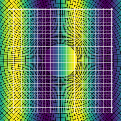
Figure 1: Equatorial slice of a wave state through the spherical global patch with a local Cartesian patch covering the origin. Black lines show the spherical grid, while white lines denote the Cartesian local patch, where every other grid line is shown.

To provide intuition into the problem at hand, we plot a scalar plane wave for the simple two patch configuration shown in Figure 1. While both patches evolve the same scalar plane wave, the coordinate representations and resolutions in which they do so are different. The global patch evolves in a discretization of spherical coordinates which excises the coordinate singularities at the origin and the pole. Meanwhile, the radially excised region is still included in the global domain by the inclusion of a Cartesian local patch. The patch executables run concurrently under the MPMD paradigm and are connected through MPI communication of boundary condition data as necessary (see Section 2.4 for full details).

Throughout the paper, unless otherwise noted, we use units in which the speed of light $c=1$. When used as tensorial indices, we reserve Greek letters (e.g., $\alpha,\beta,\gamma,\ldots$) for four-dimensional spacetime indices and Roman letters (e.g., $i,j,k,\ldots$) as indices spanning spatial dimensions. We adopt the metric sign convention of $\left(-,+,+,+\right)$ and the first index is coordinate time ($t$). We follow the Einstein summation convention where repeated upper and lower indices imply a summation. However, the index $t$ does not obey this summation convention and instead simply represents the index associated with coordinate time after splitting space and time.

2.2 Equations of Motion

We start with the standard scalar wave equation

$$\nabla^{2}\phi-\frac{1}{v^{2}}\partial^{2}_{t}\phi=S,$$ (1)

where $S$ is some scalar source term. Next, because our multipatch framework is designed to handle arbitrary coordinate systems in arbitrary frames, we recast this system to a fully covariant expression. The d’Alembertian operator, $\nabla^{2}-\frac{1}{v^{2}}\partial^{2}_{t}$, can be expressed as

$$g^{\mu\nu}\nabla_{\mu}\nabla_{\nu}\phi=S,$$ (2)

where $g^{\mu\nu}$ is the inverse metric tensor and $\nabla_{\mu}$ is the covariant derivative with respect to the metric $g_{\mu\nu}$ and coordinates $x^{\mu}$, and we set $v=c=1$. For flat spacetime and Cartesian coordinates the metric tensor and covariant derivative correspond to a $4\times 4$ matrix $\textrm{diag}\left(-1,1,1,1\right)$ and the partial derivative respectively. In A we provide a brief overview of the necessary differential geometry to understand this expression and the subsequent ones for readers unfamiliar with this notation.

We can next expand this expression in terms of only partial derivatives of the scalar wave, metric components, and Christoffel symbols of the second kind $\left({\Gamma^{\alpha}}_{\mu\nu}\right)$ as

$$S = g^{\mu\nu}\nabla_{\mu}\partial_{\nu}\phi$$

$$S = g^{\mu\nu}\left(\partial_{\mu}\partial_{\nu}\phi-{\Gamma^{\lambda}}_{\mu\nu}\partial_{\lambda}\phi\right).$$ (3)

The Christoffel symbols are themselves functions of derivatives of the metric tensor

$${\Gamma^{\alpha}}_{\mu\nu}=\frac{1}{2}g^{\alpha\lambda}\left(\partial_{\mu}g_{\lambda\nu}+\partial_{\nu}g_{\mu\lambda}-\partial_{\lambda}g_{\mu\nu}\right).$$ (4)

We now define a coordinate time $t$ that is common among all patches and explicitly split space and time.

$$S = g^{\mu t}\partial_{\mu}\partial_{t}\phi+g^{\mu i}\partial_{\mu}\partial_{i}\phi-g^{\mu\nu}\left({\Gamma^{t}}_{\mu\nu}\partial_{t}\phi+{\Gamma^{j}}_{\mu\nu}\partial_{j}\phi\right),$$

$$S = g^{tt}\partial_{t}\partial_{t}\phi+2g^{tj}\partial_{j}\partial_{t}\phi+g^{ij}\partial_{i}\partial_{j}\phi-g^{\mu\nu}\left({\Gamma}^{t}_{\mu\nu}\partial_{t}\phi+{\Gamma^{j}}_{\mu\nu}\partial_{j}\phi\right).$$ (5)

Defining a new evolved quantity, $\Pi_{t}\equiv\partial_{t}\phi$, the expressions can be further written as

$$S = g^{tt}\partial_{t}\Pi_{t}+2g^{tj}\partial_{j}\Pi_{t}+g^{ij}\partial_{i}\partial_{j}\phi-g^{\mu\nu}\left({\Gamma^{t}}_{\mu\nu}\Pi_{t}+{\Gamma^{j}}_{\mu\nu}\partial_{j}\phi\right).$$ (6)

Our interpatch communication requires the interpolation of grid functions in different coordinate systems and reference frames for arbitrary time-dependent patch configurations. We therefore will need to coordinate transform $\Pi_{t}$ between patches. We define the one-form $\Pi_{\mu}$, of which $\Pi_{t}$ is a component, as $\Pi_{\mu}=\partial_{\mu}\phi$. $\Pi_{\mu}$ obeys the standard coordinate transformation

$$\Pi_{\mu^{\prime}}=\frac{\partial x^{\lambda}}{\partial x^{\mu^{\prime}}}\Pi_{\lambda}.$$ (7)

We promote the spatial components $\Pi_{j}$ to evolved grid functions which are updated through non-coupled differential equations (preserving the second order formulation). Finally, we gather terms and simplify to obtain our complete equations of motion for the scalar wave in arbitrary coordinates, arbitrary reference frame, and any background spacetime as

$$\Pi_{t} = \partial_{t}\phi,$$ (8)

$$\partial_{t}\Pi_{t} = \frac{1}{g^{tt}}\left[S+g^{\mu\nu}\left({\Gamma^{t}}_{\mu\nu}\Pi_{t}+{\Gamma^{j}}_{\mu\nu}\partial_{j}\phi\right)-2g^{tj}\partial_{j}\Pi_{t}-g^{ij}\partial_{i}\partial_{j}\phi\right],$$ (9)

$$\partial_{t}\Pi_{i} = \partial_{i}\Pi_{t}.$$ (10)

We use the NRPy code [93, 99] to generate the centered, fourth order finite difference expressions for the right hand side (RHS) of the above evolution system.

In this framework, we may freely deploy any coordinate system or reference frame without changing our code. We always finite difference in local coordinates and account for curvature, motion, and curvilinear scale factors through a 4D coordinate transformation acting on all tensorial quantities.

2.3 Time Integration

One may write an arbitrary order Runge-Kutta (RK) time integration step for an equation of the form (see  [64])

$$\partial_{t}u\left(t,x^{i}\right)=f\left(t,x^{i}\right),$$ (11)

discretized in time by $\Delta t$, as

$$u_{n+1} = u_{n}+\Delta t\sum_{l=1}^{s}b_{l}k_{l}$$ (12)

$$k_{l} = f\left(t_{n}+c_{l}\Delta t,u_{n}+\Delta t\sum_{m=1}^{s}a_{lm}k_{m}\right).$$ (13)

Here, $u\left(t,x^{i}\right)$ is our wave state vector $u=\left[\phi,\Pi_{\mu}\right]^{T}$ and $f\left(t,x^{i}\right)$ are their associated right hand sides in Equations (8-10). We elect to use the “classic” fourth order method [100] and provide the Butcher tableau in Table 1.

0	0	0	0	0
1/2	1/2	0	0	0
1/2	0	1/2	0	0
1	0	0	1	0
	1/6	1/3	1/3	1/6

Table 1: Butcher tableau for our fourth order Runge-Kutta. The coefficients are $b_{l}$ (bottom line), $c_{l}$ (first vertical column), and $a_{lm}$ in the remainder of the table.

Recall that this code was ultimately designed to update the Einstein Field Equations (EFE) coupled to MHD. When integrating wave-like systems with the method of lines, one either needs to use partially implicit RK methods or higher than second order fully explicit RK methods, even in Cartesian coordinates [101, 102]. However, finite volume implementations of GRMHD are usually only formally second order accurate (due to the approximation of volume integrals by the midpoint rule) and furthermore drop to first order accuracy at shocks. It would be computationally wasteful to integrate the MHD equations at higher than second order in time.

We therefore write our time integration of the wave into two steps, compatible with a future mixed order integration scheme. In this scheme we first update the state vector to the half-step and return that result. We then update to the full-step. More explicitly, we update our initial wave state vector $u_{n}$ to $u_{n+1/2}$ as

$$K_{1} = f\left(t,u_{n}\right)$$ (14)

$$K_{2} = f\left(t+c_{2}\Delta t,u_{n}+a_{21}K_{1}\Delta t\right)$$ (15)

$$K_{3} = f\left(t+c_{3}\Delta t,u_{n}+a_{32}K_{2}\Delta t\right)$$ (16)

$$u_{n+1/2} = u_{n}+\Delta t\left(b_{1}K_{1}+b_{2}K_{2}+b_{3}K_{3}\right).$$ (17)

We then update $u_{n+1/2}$ to $u_{n+1}$ as

$$K_{4} = f\left(t+c_{4}\Delta t,u_{n}+a_{43}K_{3}\Delta t\right)$$ (18)

$$u_{n+1} = u_{n+1/2}+\Delta t\left(b_{4}K_{4}\right).$$ (19)

The full description of the boundary conditions we apply before calculating the slope estimates can be found in Section 2.4. To reduce high frequency noise arising from reflections at mesh refinement boundaries, we add Kreiss-Oliger dissipation [103] to the RHS of all evolved variables. An n-th order dissipation operation can be written as (see e.g. [104, 105]):

$$f\left(t,\vec{x}\right)=f\left(t,\vec{x}\right)+\left(-1\right)^{\left(n+3\right)/2}\epsilon\frac{1}{2^{n+1}}dx^{i}\partial_{i}^{n+1}u\left(t,\vec{x}\right),$$ (20)

where $\epsilon$ is the dissipation strength coefficient (set to 0.005 for this paper), and $dx^{i}$ is the cell spacing in the evenly sampled, logically Cartesian, numerical grid. To preserve the fourth order convergence of our time integration and spatial finite difference stencils, we set $n=5$ and arrive at the following addition to the RHS:

$$f\left(t,\vec{x}\right)=f\left(t,\vec{x}\right)+\epsilon\frac{1}{2^{6}}dx^{i}\partial_{i}^{6}u\left(t,\vec{x}\right).$$ (21)

2.4 Boundary Conditions

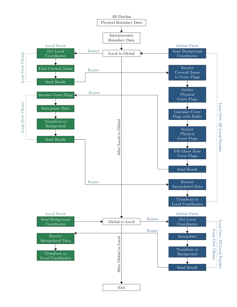
Figure 2: Flow chart for the hierarchy of boundary conditions for our code. A “client” is an individual CPU domain that lives on another patch for which this CPU is responsible. Operations in the left column are performed by local patch CPUs (colored green), the middle column by all CPUs (no color), and the right column by global patch CPUs (colored blue). We denote interpatch communication which goes through a router CPU by placing a color coded “Router” label. The color coding specifies which patch the router CPU is a member of.

A critical component of our infrastructure is the hierarchy of boundary conditions that we employ on the slope estimates $K_{1-4}$ in Equations 14-16 and 18. A version of this hierarchy was developed as part of the enhanced Patchwork code (see [1] for details), but several further modifications were necessary to facilitate arbitrary order time integration and further customization to our problem. We provide a diagram of our boundary condition procedure in Figure 2.

From Figure 2 we see that our boundary condition priority order is interpatch boundary data over interprocessor/periodic boundary data over simulation domain boundary data (analytic for our tests). We therefore lay down our boundary data into the ghost zones in the inverse of this priority order,

$$\text{Boundary Data}\to\text{Interprocessor Data}\to\text{Interpatch Data},$$

allowing interpatch boundary data to replace existing boundary conditions. By successively rewriting boundary data in this order we ensure BCs are consistent with the evolution.

Interpatch boundary conditions are applied using the Patchwork framework. Patchwork provides the ability for various local meshes, or patches, of arbitrary resolution and coordinate topology to move freely over an underlying mesh or global patch (recall our example in Figure 1). This facilitates the ability to construct local patches which are better suited to capture the physics in the encompassed area. As such, we deactivate cells on the global patch which are covered by local patches. This maintains consistency between the two patches in the overlapping region and eliminates redundant effort on the global patch.

However, the cells immediately adjacent to the local patch which are evolved on global patch require boundary conditions. These effective ghost zones are populated via interpatch interpolation from data which resides on the local patch. Similarly, the physically evolved cells on the edge of local patch require boundary conditions. These ghost zones are filled by interpatch interpolation of data which resides on the global patch. We refer to these two methods of providing boundary conditions as Local to Global and Global to Local (see Sections 2.4.2 and 2.4.1, respectively).

Interpatch data is always interpolated in the local, regular coordinate basis of the patch on which the source data resides. We apply centered fifth-order Lagrange polynomial interpolation. In 1D Lagrange polynomial interpolation can be written as

$$u(x)=\sum_{i=1}^{n+1}P_{i}(x),$$ (22)

where $u$ is the function being interpolated at location $x$, $n$ is the order of interpolation, and

$$P_{i}(x)=u(x_{i})\prod_{l=1,l\neq i}^{n+1}\frac{x-x_{l}}{x_{i}-x_{l}}.$$ (23)

Here $u(x_{i})$ is the function to be interpolated evaluated at the discrete point $x_{i}$ and sampled at points $x_{1}$ to $x_{n+1}$.

In practice, our 3D interpolation can be written as the tensor product of each dimension’s individual interpolation as

$$u(x,y,z)=\sum_{i=i_{c}-2}^{i_{c}+3}\sum_{j=j_{c}-2}^{j_{c}+3}\sum_{k=k_{c}-2}^{k_{c}+3}u_{i,j,k}P_{i}^{j,k}(x)P_{j}^{i,k}(y)P_{k}^{i,j}(z)$$ (24)

where

$$P_{i}^{j,k}(x)=\prod_{l=i_{c}-2,l\neq i}^{i_{c}+3}\frac{x-x_{l,j,k}}{x_{i,j,k}-x_{l,j,k}}.$$ (25)

We use indexing $u_{i,j,k}$ and $x_{i,j,k}$ to represent the discrete grid functions and coordinates, respectively. The $\left(i_{c},j_{c},k_{c}\right)$ indices are the closest discrete locations to the point of interpolation without exceeding it in any dimension, i.e. $\left(x,y,z\right)$ lies between $\left(x,y,z\right)_{i_{c},j_{c},k_{c}}$ and $\left(x,y,z\right)_{i_{c}+1,j_{c}+1,k_{c}+1}$. In Equation 25, we denote which index/dimension is iterated over in the product operation with the index $l$ by placing that dimension’s index as a subscript to $P$.

2.4.1 Global to Local

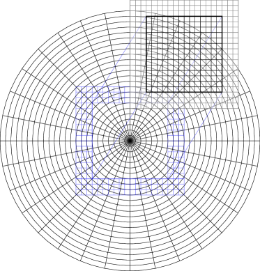
Figure 3: Schematic diagram of Global to Local interpolation zones in the equatorial plane of a spherical global patch. The local Cartesian patch, which actually resides over the origin, is offset for visualization. The solid black line denotes the edge of the physical cells on the local Cartesian mesh and gray gridlines denote physical ghost zones requiring interpatch data. The locations of these ghost zones on the global patch are marked by blue grid lines on the spherical mesh.

Although in Figure 2 we see that our algorithm first performs Local to Global, we begin our discussion with the simpler Global to Local. In the absence of overlapping local patches, the order of these BC operations is interchangeable. However, we emphasize that this interchangeability is a feature unique to the PatchworkWave version of Patchwork.

As a local patch traverses the global patch, the edges of that local patch require boundary conditions. Furthermore, because Patchwork allows dynamic patches and different coordinate topologies, coordinate locations are generally irregular with respect to the global patch mesh where the required data resides. We schematically visualize this in Figure 3 for the two patch configuration of Figure 1.

Consider a configuration with one global patch and some arbitrary number of local patches. Each CPU evolves in a numeric coordinate basis, ${X_{j}^{\alpha}}^{\prime}$. Here j refers to the patch ID, runs from $0$ to $\rm{NPATCHES}-1$, and global patch is denoted by $j=0$. Furthermore, each patch member knows the functional mapping from its numeric coordinate basis to a physical coordinate basis of the same coordinate topology, ${X_{j}^{\alpha}}\left({X_{j}^{\alpha}}^{\prime}\right)$, where $X_{j}^{\alpha}$ is either Cartesian, cylindrical, or spherical coordinates. Because each $X_{j}^{\alpha}$ is in principle irregular with respect to one another, and not known globally by all patches, all interpatch communication goes through a common background Cartesian coordinate system, $X_{B}^{\alpha}$.

Send Background Coordinates $\to$ Get Local Coordinates . In Local to Global, each local patch processor transmits its ghost zone locations, denoted by gray and blue cells in Figure 3, to the global patch CPUs (via a router - see Section 2.4.3 for discussion on parallelism) in the common background Cartesian coordinates: $X_{B}^{\alpha}\left(X_{j}^{\alpha}\right)$. Upon receiving these coordinate locations, the global patch processor transforms the points from background Cartesian to its own local numerical coordinate basis: ${X_{0}^{\alpha}}^{\prime}\left(X_{0}^{\alpha}\left(X_{B}^{\alpha}\right)\right)$.

Interpolate $\to$ Transform to Background $\to$ Send Result Global patch CPUs then attempt to locate and interpolate the state vector at each point in the ${X_{0}^{\alpha}}^{\prime}$ coordinate basis. If the data is successfully interpolated, the state vector is then transformed on the global patch processor to the background coordinates,

$${X_{0}^{\alpha}}^{\prime}\to{X_{0}^{\alpha}}\to X_{B}^{\beta},$$

and then transmitted to local patch “$j$”. Throughout the paper, we adopt the notation $X_{j}^{\alpha}\to X_{k}^{\beta}$ as representing the operation of mapping the state vector from the $X_{j}^{\alpha}$ coordinate basis to the $X_{k}^{\beta}$ coordinate basis.

Receive Interpolated Data $\to$ Transform to Local Coordinates The Local patch processor then transforms the interpolated data from the background coordinates to the local patch numerical coordinate basis:

$$X_{B}^{\alpha}\to X_{j}^{\alpha}\to{X_{j}^{\alpha}}^{\prime}.$$

If a global patch processor finds that it cannot succesfully interpolate to a point, the state vector is marked to be skipped at that point. Upon receiving the state vector on the local patch processor, only those state vectors successfully interpolated are used. Referring to Figure 2 this amounts to assuming that the point should be filled already via either physical boundary conditions or intrapatch interprocessor boundary conditions.

2.4.2 Local to Global

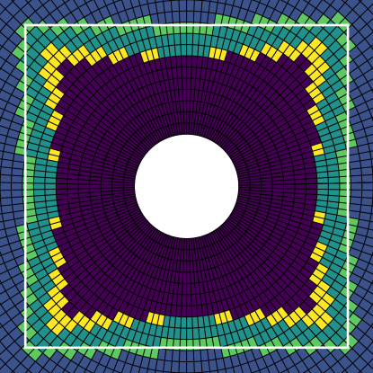
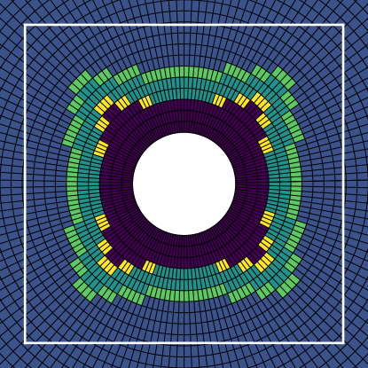
Figure 4: Example interpolation flag configuration for a Cartesian local patch over the origin of a global spherical patch in the equatorial plane. (Left) We plot the original flag implementation in [2]. (Right) We plot the new implementation with a buffer width of 4 cells. Purple zones are deactivated and play no role in the cell update, blue zones are evolved cells, and all other zones are flagged for interpatch interpolation. The white box denotes the edges of the local patch. Green cells are those which are within the ghost zone depth along any coordinate direction from evolved cells. Yellow cells are those within a ghost zone depth diagonally from evolved cells.

The other interpatch boundary condition, Local to Global, is responsible for determining which cells may be deactivated on the global patch domain as well as populating the data in the effective ghost zones underneath the local patches. This algorithm and its parallelization (see Section 2.4.3), represents the most significant departures from the original Patchwork framework.

Consider again a configuration with arbitrary number of local patches. In this scenario, we assume that no local patches overlap and can therefore treat each local patch’s interpatch BC independently. Below we describe the BC which is performed for each local patch individually.

Send Background Coordinates $\to$ Get Local Coordinates $\to$ Find Covered Zones $\to$ Send Result At the start of each timestep, the global patch processor must first ascertain which cells are covered by a local patch. For a given local patch $j$, the global patch processor first sends its coordinates in the background Cartesian frame, $X_{B}^{\alpha}\left(X_{0}^{\alpha}\right)$, to a local patch processor. The local patch processor then converts the coordinates to its own numeric coordinate basis ${X_{j}^{\alpha}}^{\prime}\left(X_{j}^{\alpha}\left(X_{B}^{\alpha}\right)\right)$. It may then ascertain which global patch cells the local patch covers, and send the result back to the global patch processor.

The reason we calculate which cells are covered on the local patch processor is because the global patch cells are generally irregular with respect to the local patch cells. Therefore, one cannot simply ask if a cell is within the bounds of the local patch coordinates. However, the local patch numerical coordinates, ${X_{j}^{\alpha}}^{\prime}$, are required by Harm3d to be regular and each global patch point, ${X_{0}^{\alpha}}$, may be determined to be within/exterior to the bounds of those regular local patch numerical coordinates.

Receive Covered Zones to Cover Flags Upon receiving the determination of which global patch cells are covered, the original Patchwork code would immediately calculate which covered cells are within an update stencil width of an uncovered cell. These global patch cells would then be flagged for interpatch interpolation. We plot the interpolation flag markers (cover flags) for our two patch example using this original algorithm in the left frame of Figure 4.

Calculate Cover Flags with Buffer However, in extending to arbitrary order methods this implementation leads to an issue. Consider that after filling the effective ghost zones in the global patch with data from the local patch, Patchwork must then call Global to Local. Looking at Figures 3 and 4, one may quickly observe that the ghost zones of the local patch would be interpolated into using data previously interpolated onto the global patch domain. This would drop the convergence of our interpolation accuracy, requiring higher order interpolation stencils and increased computational expense to overcome (both via more expensive interpolation weights and an increase in the required ghost zone count).

To overcome this limitation, we assume there exists a region of covered zones on the global patch domain capable of capturing the physics in addition to local patch. This is well posed as generally we would avoid significant cell size discrepancies at the patch boundaries to minimize numerical artifacts. In the right frame of Figure 4 we plot the same patch flag configuration including a “buffer” of evolved cells on global patch that reside immediately under the edges of the local patch. By implementing this buffer we wish to eliminate the interpolation of interpolated data present in the original Patchwork code [2].

Send Result $\to$ Receive Cover Flags $\to$ Interpolate Data Once the cells that will serve as effective ghost zones under the local patch are determined, the global patch processor sends their coordinate locations back to the local patch processor in the background Cartesian coordinates and poisons the data of fully covered cells which may be deactivated. The local patch processor then transforms the effective ghost zones to the local numerical coordinate basis, ${X_{j}^{\alpha}}^{\prime}\left(X_{j}^{\alpha}\left(X_{B}^{\alpha}\right)\right)$, and attempts to interpolate the state vector at each point in the ${X_{j}^{\alpha}}^{\prime}$ coordinate basis.

Transform to Background $\to$ Send Result If the data is successfully interpolated, the state vector is then transformed on the local patch processor to the background coordinates,

$${X_{j}^{\alpha}}^{\prime}\to X_{j}^{\alpha}\to X_{B}^{\alpha},$$

and then transmitted to the global patch processor.

Receive Interpolated Data $\to$ Transform to Local Coordinates Upon receiving the interpolated data, the global patch processor transforms the state vector to its own numerical coordinate basis:

$$X_{B}^{\alpha}\to X_{0}^{\alpha}\to{X_{0}^{\alpha}}^{\prime}.$$

Similar to Global to Local, if the point was found to be uninterpolatable, then the global patch processor skips the point and assumes that it has been previously filled by intrapatch boundary conditions.

A significant deviation of our time integration from the original Patchwork and subsequent enhanced Patchwork and PatchworkMHD codes is that we use 4th order methods. As such, we can no longer treat the timestep as two independent Cauchy problems of size $\Delta t/2$. This is because we require information about the state vector at the half-step to fully update to $t+\frac{1}{2}\Delta t$. To accommodate this, we alter the Patchwork implementation to keep constant the memory locations of live, covered, and effective ghost zones (cover flags) on the global patch processors throughout the entire timestep. The determination of which cells are live, covered, or effective ghost zones is done once the full timestep has been performed.

However, because we allow time-dependent transformations between physical and numerical coordinates on each patch, we must update these transformations when coordinate time is changed at the substeps. Additionally, because our local patches are free to move on the global patch in time, we also need to update the coordinate mappings between the global, local, and background coordinates at the same substeps. Provided these considerations, the Local to Global interpatch boundary condition at substeps is precisely that described above, but skipping the calculation of which zones are covered, live, or effective ghost.

A choice required for the Local to Global interpatch boundary condition is the specification of the buffer zone width. Our interpolation stencil extends at most $NG=3$ cells away from any given point, where $NG$ is the number of ghost zones. We therefore specify the width of the buffer of live cells underneath the local patch to $NG+1$ cells from the edges of local patch. This allows for a local patch to traverse one global patch cell during the timestep in any number of spatial dimensions. Currently, it is encumbant upon the user to verify that the specified patch trajectories do not violate this condition. However, the buffer width is a freely specifiable parameter that may also be increased to relax this constraint.

Finally, special care must be taken for physical ghost zones (ghost cells which are not interprocessor ghost zones) which are covered by a local patch. In the case of our two patch example in Figure 1, all inner radial ghost zones are covered by the local patch. These zones may be immediately adjacent to physically evolved cells, particularly in the buffer region, and will be used in cell updates. Since there is no reason to assume that the spherical BCs of the global patch match the dynamics on the Cartesian local patch, we mark all covered physical ghost zones for interpatch interpolation. This ensures that our boundary conditions are consistent with the local patch evolution, while zones which cannot be filled by interpolation will preserve the intrapatch BCs of global patch by the skipping mechanism previously described.

2.4.3 Parallelism

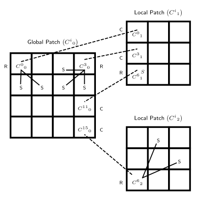
Figure 5: Reproduction of figure 3 from [2] schematically demonstrating the client-router-server paradigm for 3 patches employing multiple routers. Grids represent CPU domain decompositions. CPUs are marked as a client (C), server (S), or router (R). Solid lines connecting a router CPU to a server CPU denote intrapatch communication and dashed lines connecting a client CPU to a router CPU denote interpatch communication. Each such line denotes communication out and back between the connected CPUs.

In addition to patches being run in parallel via different executables which communicate BCs through MPI, each patch is itself MPI domain decomposed. We therefore must distinguish between interpatch and intrapatch communication. Furthermore, CPUs assigned to one patch do not know how the other patches are subdivided and assigned, and consequently do not know from which CPU to request data. Patchwork handles this transfer of data from an individual patch CPU to the appropriate CPU on another patch via a client-router-server model (for a full discussion please see [2]). Important modifications were necessary to scale well to more than a few hundred MPI ranks, and details of these changes to the original Patchwork code will be reported in [1].

Let each CPU be denoted by ${C^{i}}_{j}$, where $i$ denotes the CPU number on a given patch and $j$ denotes the patch ID. We note that we have swapped the index locations from those in [2] for consistency with our coordinate indexing in Sections 2.4.1 and 2.4.2. Patch IDs run from 0 to $N_{\rm PATCHES}-1$ and global patch is denoted with $j=0$. On any given patch, $i$ runs from 0 to ${N_{\rm CPU}}_{j}-1$ where ${N_{\rm CPU}}_{j}$ is the number of CPUs on the $j^{\mathrm{th}}$ patch.

Consider the simpler Global to Local interpatch BC. Each ghost zone on a local patch will attempt to fill its data with interpolated data from the global patch. In this instance, each ${C^{i}}_{j\neq 0}$ containing physical ghost zones becomes a “client” which requires data. However, because the client CPU does not have any knowledge of which CPU on the other patch contains the necessary data, it sends a request to the global patch via a “router” CPU. This router can distribute the requests from the client CPU to the appropriate global patch “server” ${C^{i}}_{0}$ CPUs that contain the data. Finally, the server CPUs provide the requested data and forward it back to the client CPU through the router CPU. We demonstrate this process schematically in Figure 5 (see also Figure 3 of [2]).

Similarly, when data requests are forwarded between patches in Local to Global it is transmitted from client CPUs requiring information to server CPUs containing the information via router CPUs on the server’s patch. This includes the sending of coordinates from global patch CPUs to local patch CPUs to determine which zones are covered as well as the request for interpolated data made by global patch CPUs to the local patch CPUs.

Gather Physical Cover Flags $\to$ Calculate Cover Flags with Buffer $\to$ Scatter Physical Cover Flags
Our Local to Global interpatch BC further differs from the original Patchwork implementation in the parallelization of the calculation of the effective ghost zone locations on global patch. In the original Patchwork method, each ${C^{i}}_{0}$ would calculate its own interpolation flags and then send data requests as necessary to the local patch routers at each substep. However, because our method employs a buffer extending $NG+1$ cells, each ${C^{i}}_{0}$ cannot be assumed to know the location of all patch edges required for calculating the interpolation flags.

Therefore, at the start of each timestep the global patch CPUs all forward the covered/uncovered status of their physical cells to a single global patch CPU ${C^{0}}_{0}$. ${C^{0}}_{0}$ then calculates the locations of effective ghost zones and covered states for all physical cells. We refer to physical cells as the set of cells which are a part of the computational domain, but are not a ghost cell. This information is then forwarded back to all ${C^{i}}_{0}$ to populate both physical and interprocessor ghost zone interpolation flags.

3 Code Tests

To test our code we solve the wave equation using as initial and boundary data a simple plane wave,

$$\phi\left(t,x\right)=\sin\left[\frac{2\pi}{L}\left(x-t\right)\right]+2,$$ (26)

where $L=20$ is a free parameter used to scale the period of the wave. The addition of 2 removes zero crossings to simplify the normalization of error calculations.

While in Cartesian coordinates this is a 1D problem, in curvilinear coordinates our entire covariant infrastructure is required to recover the correct solution. This is because our code always finite differences with respect to the numerical coordinate basis and uses the metric tensor and Christoffel symbols to generalize the derivatives. Additionally, the one-form $\Pi_{\mu}$ is coordinate dependent and therefore changes when solving in different coordinates/frames. Therefore, when we run multiple patches in different coordinate topologies, the entire transformation and interpolation infrastructure must also be used to correctly translate the solution in the BCs. Although symmetries may be permitted by the solution, we always run our multipatch tests in full 3D without making any symmetry assumptions. As such, by running curvilinear patches with a Cartesian problem, we test every component of our infrastructure simultaneously.

In all tests we apply analytic BCs at the physical edges of the global domain. This allows us to configure our patches arbitrarily without concern to exposed edges or proper transmissive boundaries. Furthermore, because the BCs are analytic, any reflections and errors introduces by the mesh refinements and evolution cannot be transmitted out of the domain. In setting our tests up this way, we seek to explore the “worst case scenario” where any mesh-to-mesh error/noise is unable to escape the domain and more likely to disrupt the evolution than a production simulation employing numeric/transmissive BCs.

Our timestep is always constant throughout the evolution because the numeric cell crossing time for our wave characteristic is fixed in time. Finally, we set the Kreiss-Oliger dissipation coefficient $\epsilon=0.005$ for all simulations. A small dissipation coefficient assures the damping of high frequency noise while not affecting the physical solution.

3.1 Test One

Parameter	Value
$\delta_{x1}$, $\delta_{x2}$, $\delta_{x3}$, $\delta_{x4}$	0.1
$\delta_{y1}$, $\delta_{y2}$, $\delta_{y3}$, $\delta_{y4}$	0.1
$h_{x1}$, $h_{x2}$, $h_{x3}$, $h_{x4}$	20.0
$h_{y1}$, $h_{y2}$, $h_{y3}$, $h_{y4}$	20.0
$a_{x10}$, $a_{x20}$, $a_{y10}$, $a_{y20}$	1.0
$x_{\rm min}$, $y_{\rm min}$	-20.0
$x_{\rm max}$, $y_{\rm max}$	20.0

Table 2: Parameters of the warped Cartesian grid used for our simulation. The full expressions relating these parameters are in Equations 20 and 21 of [98].

To begin, we test our wave solver independent of the Patchwork BC infrastructure. We evolve the plane wave solution of Equation 26 in a time-dependent double fish-eye warped Cartesian coordinate system [98]. In this coordinate system there are two regions of dynamic warping which orbit counter-clockwise at an orbital frequency of $\Omega_{\rm warp}=\pi/50$. We tabulate the parameters of the warped grid in Table 2.

For this study (and in our upcoming paper about PatchworkMHD [1]), we implemented the infrastructure to map any spacetime known by Harm3d from a background reference frame to some arbitrary time-dependent reference frame. The background frame here would correspond to $X_{B}^{\alpha}$ in the Patchwork infrastructure. Specifically, we pass the background coordinates to the routines responsible for evaluating the metric, which then transform the resultant metric tensor via

$$X_{B}^{\alpha}\to X_{\rm rotating}^{\alpha}\to X_{\rm WARPED}^{\alpha}.$$

In addition to testing the dynamic coordinate and covariant infrastructure of the wave solver, we wish to test this generalized frame infrastructure. To do this, we place the mesh into a frame rotating clockwise at a frequency of $\Omega_{\rm frame}=0.01$ about the $z$ axis with respect to the background coordinates. That is,

$$\frac{\partial}{\partial X_{B}^{\alpha}}X_{\rm rotating}^{\alpha}=\begin{bmatrix}\cos\left(\Omega t\right)&\sin\left(\Omega t\right)&0\\ -\sin\left(\Omega t\right)&\cos\left(\Omega t\right)&0\\ 0&0&1\end{bmatrix},$$ (27)

where $\Omega=\Omega_{\rm frame}$.

As we are not employing the full interpatch BCs and only testing the enhanced Patchwork coordinate and Harm3d metric modifications in conjunction with our wave solver, we run this test in 2D. Our grid contains $100\times 100$ cells, producing a numerical cell size of $dx^{1}=dx^{2}=0.01$. We set the timestep to half this numerical cell size: $dt=0.005$. The simulation domain extends from $-20$ to $20$ in $x$ and $y$ in the local rotating frame. We normalize the wave period of Equation 26 by setting $L=20$. This test employs every component of the generalized coordinate/metric infrastructure within the $x-y$ plane.

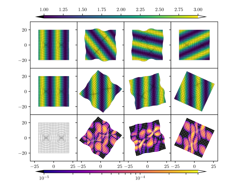
Figure 6: (Top Row) Time snapshots of the wave plotted with respect to the rotating frame coordinates used during the update. (Middle Row) Time snapshots of the wave plotted with respect to the fixed background coordinates. (Bottom Row) Logarithmic relative error in the wave plotted with respect to the fixed background coordinates. We do not plot the initial error because it is zero to machine precision. (Left to Right) Time snapshots correspond to $t=0$, $t=66.5$, $t=133$, and $t=200$. We overlay every 5th gridline of the mesh.

We evolve for 5 wave crossing times of our simulation domain, or two complete rotations of the warps, ($t=200$) and plot snapshots of the evolution in Figure 6. We find that even though the warps strongly distort the grid from the symmetry of the wave solution, our relative error remains small (of order several $\times 10^{-4}$). Furthermore, the top two rows, which show the evolution plotted against the rotating frame coordinates and fixed background coordinates, highlight that the wave propagation direction rotates counter-clockwise in the numerical coordinate basis where the evolution is performed. This propagation direction time dependence is encoded in the structure of $\Pi_{\mu}$. Finally, the values of $\Pi_{\mu}$ are further altered and distorted to account for the warps in the mesh on which the wave is updated.

3.2 Test Two

While the original Patchwork code was designed to work with second order time integration and linear interpolation for interpatch BCs (recall the additional issue of interpolation of interpolated data further reducing the convergence order), we have modified Patchwork to be compatible with arbitrary order methods in space and time.

We test the convergence rate of PatchworkWave using a Cartesian local patch which is fully encompassed by a global Cartesian patch with a mesh refinement level of 2-to-1. The global patch cube extends from $-20$ to $20$ in each dimension and the local patch cube extends from $-10$ to $10$ in local coordinates $X_{1}^{i}$. In all cases the resolution in each dimension is equal and we employ a Courant-Friedrichs-Lewy (CFL) factor of 0.6 to determine the timestep.

We perform three tests; a fixed local patch, a dynamically rotating local patch, and a linearly translating local patch. For the fixed local patch, we set the origin of the local patch to $\left(x,y,z\right)=\left(-1,-1,-1\right)$ to ensure that the local patch grid is offset from the global patch grid. For the rotating local patch, we set the local patch origin at the global patch origin and rotate counter-clockwise at a frequency of 0.01 about the z axis. For the translating local patch, we set the initial local patch origin at $\left(x,y,z\right)=\left(-5,-5,0\right)$ and linearly translate with a velocity of $v^{i}=\left(0.1,0.1,0\right)$. In all cases we evolve for 1 wave crossing time of the fixed local patch, $t=20$, which coincides with the wave period.

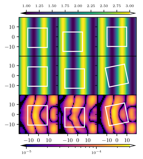
Figure 7: (Top Row) Initial configuration of the wave for our convergence study at the lowest resolution sampled. (Middle Row) Final configuration of the wave for our convergence study at the lowest resolution sampled. (Bottom Row) Logarithmic relative error in the wave at the end of the simulation for our lowest resolution sampled. (Left to Right) We plot the fixed local patch, translating local patch, and rotating local patch configurations. All plots are in the x-y plane at a slice of $z=0$. The edge of the local patch is denoted by the white box. Global patch resolution is $dx=dy=dz=1$ and local patch resolution is $dx=dy=dz=0.5$.

In Figure 7 we plot snapshots of the initial and final configuration of the wave, as well as the relative error in the final state, for each patch configuration at the lowest resolution sampled. Just like in the warped configuration, we find that the relative error is small at the end of the simulation (of order several $\times 10^{-4}$) even at a resolution of $dx=dy=dz=1$ on global patch. Additionally, we note that the error is continuous across the patch boundaries, showing negligible to no distortions due to transportation onto and off of the mesh refinement of local patch. We note that the peak of the wave has both transported off of and back onto the local patch during our test.

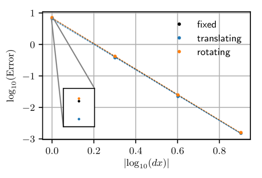
Figure 8: Total integrated relative error on both patches for our three convergence tests. Points denote the value for each resolution and the dashed line is a linear fit to the data. We include an inset of the lowest resolution points to highlight that they are distinctly separate. The size of the inset is not drawn to scale. The slopes are; fixed -4.06, translating -4.03, and rotating -4.05.

To confirm the convergence rate of our algorithm, we sample 4 resolutions differing by a factor of 2. In such a configuration, for our globally 4th order scheme, the error should reduce by a factor of 16 for each resolution increase.

We measure our convergence rate by calculating the total integrated error in the simulation domain

$$\rm{Error}=\int\frac{\left|\phi-\phi_{\rm analytic}\right|}{\phi_{\rm analytic}}\sqrt{-g}\,d^{3}x,$$ (28)

for all physically evolved cells on both patches. Here, $\sqrt{-g}$ is the determinant of the metric tensor and generalizes the Jacobian term in front of the differentials. In Figure 8 we plot this integrated error at the end of the simulation for all three tests on a log-log scale. On this scale, the convergence order of the error is the linear slope of the data ($\times$ -1).

Two things are quickly apparent from the plot. First, the global convergence order of PatchworkWave with our modifications is precisely the 4th order convergence rate we desired. Second, the global integrated error between each simulation is comparable at all resolutions. This implies that the total error of our scheme is relatively insensitive the location and trajectory of our refined local patch for this test. Instead, the error is dominated by the 4th order spatial finite difference stencils and time integration performed locally. Furthermore, the effectiveness of our algorithm is exemplified by the rotating patch mesh breaking with the symmetry of the plane wave in a time-dependent manner. Finally, with the dynamic patch configurations we demonstrate the ability to dynamically cover/uncover cells throughout the evolution with our modifications to interpatch ghost zone mapping routines while preserving the desired convergence properties.

3.3 Test Three

We now perform a test which includes three patches with one of each coordinate topology; Cartesian, spherical, and cylindrical. In this test the local patches both dynamically evolve in time with respect to the global patch. Furthermore, we intentionally configure the patches in a manner to make interpatch reflections highly pronounced.

The global Cartesian grid has dimensions of $x\times y\times z=80\times 80\times 40$ with its origin at $\left(x,y,z\right)=\left(0,0,0\right)$. We sample the domain with $160\times 160\times 40$ cells. The spherical local patch is centered at $\left(x,y,z\right)=\left(-22,0,0\right)$. The uniform radial grid extends from $5$ to $20$, poloidal angle from $\pi/4$ to $3\pi/4$, and we include the full $2\pi$ in azimuthal angle. We sample the spherical domain with $\left(r,\theta,\phi\right)=30\times 40\times 200$ cells. The cylindrical local patch is centered at $\left(x,y,z\right)=\left(22,0,0\right)$. The radial domain and azimuthal domain extents are the same as the spherical patch. The vertical extent of the cylindrical patch is half that of the global Cartesian patch. The cylindrical domain is sampled with $\left(r,\phi,z\right)=30\times 200\times 20$ cells. Finally, the spherical patch rotates counter-clockwise at a frequency of 0.01 and the cylindrical patch rotates clockwise at a frequency of 0.03 (both with respect to their local z axes).

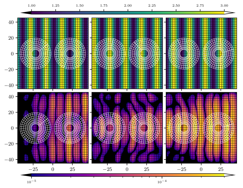
Figure 9: (Top) Snapshots in the x-y plane for the run at $z=0$. (Bottom) Relative error in the x-y plane at $z=0$. (Left to Right) Time snapshots correspond to $t=66.5$, $t=133$, and $t=200$. We overlay every 5th gridline of the meshes.

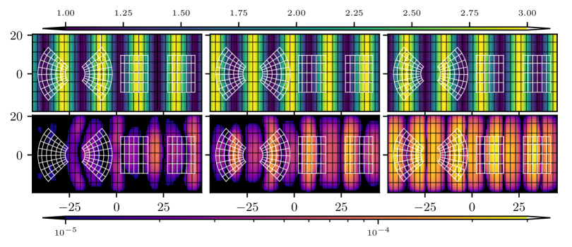
Figure 10: (Top) Snapshots in the x-z plane for the run at $y=0$. (Bottom) Relative error in the x-z plane at $y=0$. (Left to Right) Time snapshots correspond to $t=66.5$, $t=133$, and $t=200$. We overlay every 5th gridline of the meshes.

In Figure 9 we plot snapshots of the wave and relative error in the $x-y$ plane through our evolution. In these snapshots at $z=0$ the resolution of the spherical and cylindrical meshes are identical. However, the azimuthal phase of the local coordinates, along with the Jacobians relating the local patch and global patch coordinates, are different. Additionally, we plot the same snapshots in the $x-z$ plane in Figure 10. The selection of $y=0$ for this slice was made to represent one of the most error prone slices in the domain. Observing the lower panels of Figures 9 and 10 we find that the relative error grows in time to $\mathcal{O}\left(10^{-4}\right)$. Had we continued the evolution, the error would likely continue to increase.

However, this test was precisely designed to exacerbate errors associated with propagating the wave through mesh refinement. For instance, the wave must cross mesh refinement boundaries 8 times for $\left|y\right|\mathrel{\hbox{\hbox to0.0pt{\hbox{\lower 4.0pt\hbox{$\sim$}}\hss}\hbox{$<$}}}5$. Furthermore, no special care was taken to reduce the factor of cell refinement between meshes in any portion of the domain and the local patches do not conform to the symmetry of the plane wave. Finally, we intentionally placed the local patch edges immediately adjacent to the outer edges of the global patch along the direction of propagation. This last part is important because the analytic BCs we apply act like a reflective boundary for any error modes generated by the mesh refinements and intrapatch truncation error.

Provided these considerations, we believe that the relative error growing to only $\mathcal{O}\left(10^{-4}\right)$ is a strong testament to the effectiveness of our interpatch BCs. We emphasize that any production simulation employing the Patchwork infrastructure would likely have more transmissive boundary conditions and would place meshes to better capture the physics rather than infringe on the algorithm’s ability to obtain an accurate solution as we did here.

3.4 Test Four

To fully demonstrate PatchworkWave’s mesh capabilities, we perform another test which includes three patches with one of each coordinate topology. In this test we include one translating patch, one rotating patch, a curvi-linear global patch, and allow the local patches to overlap in the buffer regions.

The global spherical grid extends from $r_{\rm in}=5$ to $r_{\rm out}=100$, poloidally from $\pi/4$ to $3\pi/4$, and includes the full azimuthal domain. We uniformly sample the domain with $r\times\theta\times\phi=100\times 100\times 300$ cells. We include a Cartesian patch centered over the radial cutout which has dimensions of $x\times y\times z=30\times 30\times 20$ and sampled with $80\times 80\times 20$ cells. The patch rotates counter-clockwise in time at a frequency of 0.03 about the z-axis. The cylindrical patch extends radially from $r_{\rm in}=5$ to $r_{\rm out}=25$, from -10 to 10 in the $z$ direction, and includes the full azimuthal angle. When speaking of spherical coordinates we always refer to spherical radius. Conversely, when we are referring to a cylindrical coordinate system we refer to cylindrical radius. We offset the initial position of the cylindrical patch from the global spherical patch origin by $\left(x,y,z\right)=\left(45,45,0\right)$. We then translate the cylindrical patch at a velocity of -0.5 in the x direction. We specify the simulation timestep to $dt=0.05$.

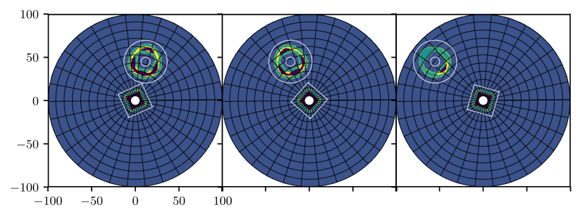
Figure 11: (Top) Snapshots of the interpatch interpolation flags in the x-y plane for the run at $z=0$. (Left to Right) Time snapshots correspond to $t=66.5$, $t=133$, and $t=200$. We overlay every 10th gridline of the global patch mesh and the outer physical boundaries of the local patch meshes. Purple denotes deactivated cells, blue evolved cells, and all other colors an interpatch interpolation zone.

We evolve two wave solutions in this setup until $t=200$, allowing the cylindrical patch to fully traverse the spherical global patch in the equatorial plane. Unlike the test presented in Section 3.3, the interpolation flags identifying which zones require interpatch interpolated data must be dynamically updated in addition to the coordinate mappings relating the patches. We demonstrate this in Figure 11, where we show that, unlike Cartesian local patches which only have buffers cells outside the covered zones, the cylindrical patch must have buffer cells extending from both of their inner radial boundaries. Furthermore, the number of cells under the local cylindrical patch which may be deactivated increases as the patch extends deeper into the spherical global patch radial domain. This emphasizes that, in general, the amount of work a given patch must do, as well as the structure of the deactivated, live, and interpolated cells, must be accounted for dynamically and can vary significantly based on the mesh configurations at any timestep.

3.4.1 Single Plane Wave

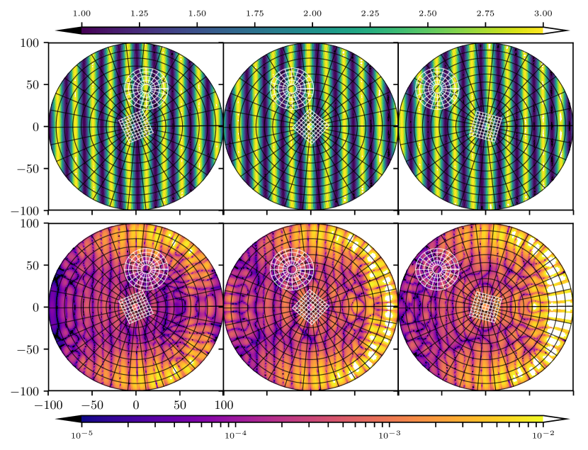
Figure 12: (Top) Snapshots in the x-y plane for the run at $z=0$. (Bottom) Relative error in the x-y plane at $z=0$. (Left to Right) Time snapshots correspond to $t=66.5$, $t=133$, and $t=200$. We overlay every 10th gridline of the meshes.

In Figure 12 we plot snapshots of the simple 1D plane wave solution and relative error in the equatorial $\theta=\pi/2$ plane of the global patch and $z=0$ plane of the local patches. Unlike our previous simulations, we note that the maximal global error of the simulation is significantly higher. However, we emphasize that this is due to the decreased effective resolution of the global spherical patch at large radii. Furthermore, because error generated in the very coarse cells at $\phi=\pi/2$ and $\phi=3\pi/2$ ($dx\approx rd\phi\approx 2.1$) cannot escape the domain with our analytic BCs, it is funneled along the outer radial boundary to the $\phi\approx 0$ boundary where the plane wave propagates off the domain.

Furthermore, at $t\approx 75$, between snapshots 1 and 2 in the Figures, the corner of the rotating Cartesian local patch penetrates through the cylindrical outer boundary. At these times the physical ghost zones from both patches draw interpolated data from the buffer regions under the other local patch. While our algorithm does not allow live or buffer cells in local patches to be covered by other local patches, it does allow their ghost zone regions to overlap.

3.4.2 Superposition of Plane Waves

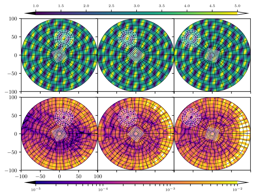
Figure 13: (Top) Snapshots in the x-y plane for the run at $z=0$. (Bottom) Relative error in the x-y plane at $z=0$. (Left to Right) Time snapshots correspond to $t=66.5$, $t=133$, and $t=200$. We overlay every 10th gridline of the meshes.

Finally, to demonstrate that the 1D nature of our simple plane wave is not exploited by our code, we evolve a superposition of two plane waves in the same patch configuration. Each wave has a different wave vector and frequency. Specifically, we evolve

$$\phi\left(t,x,y,z\right) = \sin\left[\frac{2\pi}{L_{1}}\left(x-t\right)\right]+\cos\left[\frac{2\pi}{L_{2}}\left(x-y+z-\sqrt{3}t\right)\right]+3,$$ (29)

where we set $L_{1}=20$ and $L_{2}=30$. This solution requires resolving full 3D wave propagation and two independent wave periods simultaneously. We plot a slice at $z=0$ for the same time snapshots as in the previous section in Figure 13.

In the figure we note that the wave features which our code must resolve are quite different from the single plane wave solution. However, by comparing snapshots in Figures 12 and 13, we observe that the overall magnitude of the error is comparable. This demonstrates that, so long as the grid is sufficiently sampled to resolve the gradients of the solution, our error is dominated by the truncation error of our spatial and temporal discretization.

4 Conclusions

We have described extensions to the Patchwork [2] and enhanced Patchwork [1] (upon which this code is built) framework necessary for this study, high-order finite difference methods, as well as those developed jointly for this publication and with the new MHD-capable code PatchworkMHD [1]. We have additionally described in detail some of the underlying enhanced Patchwork infrastructure for clarity.

We have extended the framework to be multimethod compatible, improved the accuracy of interpatch BCs, and removed assumptions pertaining to finite volume fluid evolutions. These extensions were motivated by a multimethod astrophysics application coupling numerical solutions to the EFE via finite difference methods, to the evolution of the MHD equations employing finite volume methods. As the original Patchwork has already been successfully employed for fluid evolutions in  [2], and its MHD counterpart is currently being deployed  [106], we have demonstrated only the finite difference component here through the evolution of a scalar wave toy-model. We implemented this toy-model into the Harm3d code.

While there is certainly MPI overhead associated with our infrastructure, the exact cost is difficult to predict, as well as often specific to the simulation or application. For instance, the relative expense of interpatch interpolation to the time integration of the state vector, the number of cells which require interpolation, the fraction of deactivated cells on a patch, the cell count disparity between various patches, and each patch’s domain decomposition all play a role. We therefore do not expect the overhead associated with our toy-model to necessarily be a good predictor for another application. As such, we have left a full discussion of the scaling and overhead to a future publication which is optimized to its target application.

However, we emphasize that the extreme flexibility of Patchwork allows users to develop meshes that are custom tailored to minimize cell count, maximize timestep, and completely remove many-level nested box-in-box AMR. These benefits, when combined with arbitrary patch motion, have the potential to far outweigh the overhead costs. For instance, PatchworkMHD is currently being deployed to efficiently extended the simulation of SMBBH accretion presented in  [38, 39] from 12 to 30 binary orbital periods at a fraction of the computational cost  [106]. Furthermore, because each application code is itself parallelized, users may domain decompose their application code as they see fit to limit communication overhead.

In addition to the simplicity of implementation, a second order formulation of the scalar wave has stability criteria similar to many other applications in computational physics. Applications of wave-like systems span general relativity to quantum mechanics. Although we elected to implement a coordinate invariant form of the wave equation using a metric tensor, we emphasize that this is not a critical component of the new Patchwork infrastructure. Furthermore, our code would be equally capable of evolving another set of hyperbolic PDEs at arbitrary order. The only necessary ingredients are a time integrator for the equations, an interpolator, a method of identifying neighboring cells, and coordinate transformation rules for the state vector.

Our expansions allow for the new enhanced Patchwork code (and hence both PatchworkWave and PatchworkMHD) to be compatible with a wide range of infrastructures beyond finite difference or finite volume. For instance, our infrastructure could be coupled to any number of integration methods, where each application provides the necessary methods listed above. In principle, the code we present here could even be coupled to non-hyperbolic PDEs, such as an elliptic multigrid solver, where Patchwork would provide intergrid interpolation at some iteration frequency.

Through our toy-model, we have demonstrated that the further enhanced Patchwork infrastructure may be deployed to produce a generic multipatch scheme which is globally convergent at the order of the mesh/temporal discretization. This is facilitated by our improvements to the interpatch interpolation, introduction of an arbitrary size buffer region, and the capability of handling multiple state vectors simultaneously (each employing their own interpatch interpolation/transformation procedures). With these extensions, Patchwork promises to provide accurate solutions for physics applications which have disparate resolution/physics requirements, different numerical technique requirements, and allows for moving mesh advantages even in the presence of complex solution geometries. Finally, this proof of principle calculation represents a significant step towards the goal of time-dependent multipatch schemes in numerical relativity.

Appendix A Coordinate Invariant Wave Equation

In order to understand how our code handles the generalization of motions and coordinates, a basic understanding of tensor calculus on manifolds is required. We present here a very basic introduction for readers unfamiliar with tensor calculus so as to understand the origins of the equations presented in Section 2.2. For more background information see  [107].

Consider a 4-dimensional Riemannian manifold (time + space). This manifold may have arbitrary curvature and may be spanned using any freely specifiable coordinate basis vectors $e_{\mu}$. In this situation, the differential distance between points $(ds^{2})$ may be expressed in a coordinate invariant manner as

$$ds^{2}=\sum_{\mu=1}^{4}\sum_{\nu=1}^{4}g_{\mu\nu}dx^{\mu}dx^{\nu},$$ (30)

where repeated upper and lower Greek indices always imply a sum over all 4 spacetime indices (from here we drop the explicit summation symbol) and $g_{\mu\nu}$ is the metric tensor of the 4-dimensional manifold. In the Cartesian representation of flat (Minkowski) spacetime, our indexing corresponds to $x^{\mu}=\left(t,x,y,z\right)$ and the metric tensor, $g_{\mu\nu}=\textrm{diag}\left(-1,1,1,1\right)$, recovers the standard Lorentzian displacement formula: $\left|\vec{x}^{\prime}-\vec{x}\right|=\sqrt{-\left(x_{1}^{\prime}-x_{1}\right)^{2}+\sum_{i=2}^{4}\left(x_{i}^{\prime}-x_{i}\right)^{2}}$. The metric tensor obeys the standard tensorial transformation law of

$$g_{\mu^{\prime}\nu^{\prime}}=\frac{\partial x^{\mu}}{\partial x^{\mu^{\prime}}}\frac{\partial x^{\nu}}{\partial x^{\nu^{\prime}}}g_{\mu\nu}.$$ (31)

It may be trivially shown that for spherical $\left(t,r,\theta,\phi\right)$ and cylindrical $\left(t,r,\phi,z\right)$ coordinates the flat spacetime (Minkowski) metric tensor becomes $g_{\mu\nu}=\textrm{diag}\left(-1,1,r^{2},r^{2}\sin\theta\right)$ and $g_{\mu\nu}=\textrm{diag}\left(-1,1,r,1\right)$ respectively.

Additionally, in deriving our EOM we generalize the partial derivative operator. The generalized form of differentiation, the covariant derivative, correctly accounts for curvilinear scale factors as well as curvature. By definition, the covariant derivative acting on the metric tensor is always zero. Under this assumption, the covariant derivative acting on a scalar function is precisely the partial derivative operator. However, for tensorial quantities (such as $\partial_{\mu}\phi=\Pi_{\mu}$) it may be shown that the derivative of an arbitrary tensor of rank $n\times m$ along coordinate $x^{\mu}$ is

$$\nabla_{\mu}{T^{\alpha_{1}\cdots\alpha_{n}}}_{\beta_{1}\cdots\beta_{m}} = \partial_{\mu}{T^{\alpha_{1}\cdots\alpha_{n}}}_{\beta_{1}\cdots\beta_{m}}$$

$$\,+{\Gamma^{\alpha_{1}}}_{\mu\lambda}{T^{\lambda\alpha_{2}\cdots\alpha_{n}}}_{\beta_{1}\cdots\beta_{m}}+{\Gamma^{\alpha_{2}}}_{\mu\lambda}{T^{\alpha_{1}\lambda\cdots\alpha_{n}}}_{\beta_{1}\cdots\beta_{m}}+\cdots+{\Gamma^{\alpha_{n}}}_{\mu\lambda}{T^{\alpha_{1}\alpha_{2}\cdots\lambda}}_{\beta_{1}\cdots\beta_{m}}$$

$$\,-{\Gamma^{\lambda}}_{\mu\beta_{1}}{T^{\alpha_{1}\cdots\alpha_{n}}}_{\lambda\beta_{2}\cdots\beta_{m}}-{\Gamma^{\lambda}}_{\mu\beta_{2}}{T^{\alpha_{1}\cdots\alpha_{n}}}_{\beta_{1}\lambda\cdots\beta_{m}}-\cdots-{\Gamma^{\lambda}}_{\mu\beta_{m}}{T^{\alpha_{1}\cdots\alpha_{n}}}_{\beta_{1}\beta_{2}\cdots\lambda}.$$

Here ${\Gamma^{\alpha}}_{\mu\nu}$ are the Christoffel symbols of the second kind, or connection coefficients, and may be expressed in terms of the metric tensor as

$${\Gamma^{\alpha}}_{\mu\nu}=\frac{1}{2}g^{\alpha\lambda}\left(\partial_{\mu}g_{\lambda\nu}+\partial_{\nu}g_{\mu\lambda}-\partial_{\lambda}g_{\mu\nu}\right).$$ (33)

$g^{\mu\nu}$ is the inverse metric tensor which may be obtained by taking the inverse matrix representation of the $4\times 4$ metric tensor $g_{\mu\nu}$.

In deriving and relating our expressions, it is important to note that the location of indices (upper vs lower indices) in this notation must be respected. The traditional vector representation of a one-form $\Pi_{\mu}$ may be found by “raising” the index with the metric tensor

$$\Pi^{\mu}=g^{\mu\lambda}\Pi_{\lambda}.$$ (34)

Conversely, the one-form may be found from the vector by “lowering” the index with the metric tensor

$$\Pi_{\mu}=g_{\mu\lambda}\Pi^{\lambda}.$$ (35)

This may be performed for any number of indices, with each index obeying one of the two expressions above.

Finally, covariant expressions may be obtained by replacing partial derivatives with covariant derivatives. That is, the laplacian operator in Cartesian coordinates $\nabla^{2}=\sum_{i}\partial_{i}^{2}=\partial^{i}\partial_{i}$ may be obtained by first lowering the first index

$$\nabla^{2}=g^{ij}\partial_{i}\partial_{j},$$ (36)

where repeated latin indices only sum over spatial indices of the manifold ($(x,y,z)$, $(r,\theta,\phi)$, $(r,\phi,z)$ etc.). Next, partial derivatives are replaced with their covariant generalization producing

$$\nabla^{2}=g^{ij}\nabla_{i}\nabla_{j}.$$ (37)

Finally, for convenience, we set the wave speed to the speed of light. We may then absorb the $-\partial_{t}\partial_{t}\phi$ term into a 4 dimensional sum with the metric tensor and define the fully coviariant wave expression presented in Equation 2.

References

- Avara, M.J., Bowen, D.B., Ryu, T., Noble, S.C., Mewes, V., Krolik, J.H., Campanelli, M. [2020] Avara, M.J., Bowen, D.B., Ryu, T., Noble, S.C., Mewes, V., Krolik, J.H., Campanelli, M., PatchworkMHD: A Multipatch Infrastructure for MHD Simulations (2020).
- Shiokawa et al. [2018] H. Shiokawa, R. M. Cheng, S. C. Noble, J. H. Krolik, PATCHWORK: A Multipatch Infrastructure for Multiphysics/Multiscale/Multiframe Fluid Simulations, Astrophysical Journal 861 (2018) 15. doi:10.3847/1538-4357/aac2dd.
- Gomez et al. [2014] M. R. Gomez, S. A. Slutz, A. B. Sefkow, D. B. Sinars, K. D. Hahn, S. B. Hansen, E. C. Harding, P. F. Knapp, P. F. Schmit, C. A. Jennings, T. J. Awe, M. Geissel, D. C. Rovang, G. A. Chandler, G. W. Cooper, M. E. Cuneo, A. J. Harvey-Thompson, M. C. Herrmann, M. H. Hess, O. Johns, D. C. Lamppa, M. R. Martin, R. D. McBride, K. J. Peterson, J. L. Porter, G. K. Robertson, G. A. Rochau, C. L. Ruiz, M. E. Savage, I. C. Smith, W. A. Stygar, R. A. Vesey, Experimental demonstration of fusion-relevant conditions in magnetized liner inertial fusion, Phys. Rev. Lett. 113 (2014) 155003. doi:10.1103/PhysRevLett.113.155003.
- Frank et al. [2002] J. Frank, A. King, D. J. Raine, Accretion Power in Astrophysics: Third Edition, 2002.
- Janka et al. [2007] H.-T. Janka, K. Langanke, A. Marek, G. Martínez-Pinedo, B. Müller, Theory of core-collapse supernovae, Physics Reports 442 (2007) 38–74. doi:10.1016/j.physrep.2007.02.002.
- Springel et al. [2005] V. Springel, S. D. M. White, A. Jenkins, C. S. Frenk, N. Yoshida, L. Gao, J. Navarro, R. Thacker, D. Croton, J. Helly, J. A. Peacock, S. Cole, P. Thomas, H. Couchman, A. Evrard, J. Colberg, F. Pearce, Simulations of the formation, evolution and clustering of galaxies and quasars, Nature 435 (2005) 629–636. doi:10.1038/nature03597.
- Ivanova et al. [2013] N. Ivanova, S. Justham, X. Chen, O. De Marco, C. L. Fryer, E. Gaburov, H. Ge, E. Glebbeek, Z. Han, X.-D. Li, G. Lu, T. Marsh, P. Podsiadlowski, A. Potter, N. Soker, R. Taam, T. M. Tauris, E. P. J. van den Heuvel, R. F. Webbink, Common envelope evolution: where we stand and how we can move forward, The Astronomy and Astrophysics Review 21 (2013) 59. doi:10.1007/s00159-013-0059-2.
- Sanderse et al. [2011] B. Sanderse, S. van der Pijl, B. Koren, Review of computational fluid dynamics for wind turbine wake aerodynamics, Wind Energy 14 (2011) 799–819. doi:10.1002/we.458.
- Abbott et al. [2016a] B. P. Abbott, R. Abbott, T. D. Abbott, M. R. Abernathy, F. Acernese, K. Ackley, C. Adams, T. Adams, P. Addesso, R. X. Adhikari, V. B. e. a. Adya (LIGO Scientific Collaboration and Virgo Collaboration), Observation of gravitational waves from a binary black hole merger, Phys. Rev. Lett. 116 (2016a) 061102. doi:10.1103/PhysRevLett.116.061102.
- Abbott et al. [2016b] B. P. Abbott, et al. (Virgo, LIGO Scientific), GW151226: Observation of Gravitational Waves from a 22-Solar-Mass Binary Black Hole Coalescence, Phys. Rev. Lett. 116 (2016b) 241103. doi:10.1103/PhysRevLett.116.241103.
- Abbott et al. [2017] B. P. Abbott, R. Abbott, T. D. Abbott, F. Acernese, K. Ackley, C. Adams, T. Adams, P. Addesso, R. X. Adhikari, V. B. e. a. Adya (LIGO Scientific and Virgo Collaboration), Gw170104: Observation of a 50-solar-mass binary black hole coalescence at redshift 0.2, Phys. Rev. Lett. 118 (2017) 221101. doi:10.1103/PhysRevLett.118.221101.
- Abbott et al. [2017] B. P. Abbott, R. Abbott, T. D. Abbott, F. Acernese, K. Ackley, C. Adams, T. Adams, P. Addesso, R. X. Adhikari, V. B. e. a. Adya, GW170608: Observation of a 19 Solar-mass Binary Black Hole Coalescence, Astrophysical Journal, Letters 851 (2017) L35. doi:10.3847/2041-8213/aa9f0c.
- Abbott et al. [2018a] B. P. Abbott, et al. (LIGO Scientific, Virgo), GWTC-1: A Gravitational-Wave Transient Catalog of Compact Binary Mergers Observed by LIGO and Virgo during the First and Second Observing Runs (2018a). arXiv:1811.12907.
- Abbott et al. [2018b] B. P. Abbott, et al. (LIGO Scientific, Virgo), Binary Black Hole Population Properties Inferred from the First and Second Observing Runs of Advanced LIGO and Advanced Virgo (2018b). arXiv:1811.12940.
- Kara et al. [2019] E. Kara, R. Margutti, A. Keivani, W.-f. Fong, B. Cenko, S. Noble, R. Mushotzky, J. Ruan, G. Ryan, E. Burns, D. Haggard, R. Caputo, D. Fox, D. Burrows, X-ray follow-up of extragalactic transients, arXiv e-prints (2019) arXiv:1903.05287. arXiv:1903.05287.
- Baker et al. [2019] J. Baker, Z. Haiman, E. M. Rossi, E. Berger, N. Brandt, E. Breedt, K. Breivik, M. Charisi, A. Derdzinski, D. J. D’Orazio, S. Ford, J. E. Greene, J. C. Hill, K. Holley-Bockelmann, J. S. Key, B. Kocsis, T. Kupfer, S. Larson, P. Madau, T. Marsh, B. McKernan, S. T. McWilliams, P. Natarajan, S. Nissanke, S. Noble, E. S. Phinney, G. Ramsay, J. Schnittman, A. Sesana, D. Shoemaker, N. Stone, S. Toonen, B. Trakhtenbrot, A. Vikhlinin, M. Volonteri, Multimessenger science opportunities with mHz gravitational waves, arXiv e-prints (2019) arXiv:1903.04417. arXiv:1903.04417.
- Krolik [2010] J. H. Krolik, Estimating the Prompt Electromagnetic Luminosity of a Black Hole Merger, Astrophysical Journal 709 (2010) 774–779. doi:10.1088/0004-637X/709/2/774.
- MacFadyen and Milosavljević [2008] A. I. MacFadyen, M. Milosavljević, An Eccentric Circumbinary Accretion Disk and the Detection of Binary Massive Black Holes, Astrophysical Journal 672 (2008) 83–93. doi:10.1086/523869.
- Shi et al. [2012] J.-M. Shi, J. H. Krolik, S. H. Lubow, J. F. Hawley, Three-dimensional magnetohydrodynamic simulations of circumbinary accretion disks: Disk structures and angular momentum transport, The Astrophysical Journal 749 (2012) 118. URL: http://stacks.iop.org/0004-637X/749/i=2/a=118.
- D’Orazio et al. [2013] D. J. D’Orazio, Z. Haiman, A. MacFadyen, Accretion into the central cavity of a circumbinary disc, Monthly Notices of the Royal Astronomical Society 436 (2013) 2997–3020. doi:10.1093/mnras/stt1787.
- Farris et al. [2014] B. D. Farris, P. Duffell, A. I. MacFadyen, Z. Haiman, Binary Black Hole Accretion from a Circumbinary Disk: Gas Dynamics inside the Central Cavity, The Astrophysical Journal 783 (2014) 134. doi:10.1088/0004-637X/783/2/134.
- Farris et al. [2015a] B. D. Farris, P. Duffell, A. I. MacFadyen, Z. Haiman, Binary black hole accretion during inspiral and merger, Monthly Notices of the RAS 447 (2015a) L80–L84. doi:10.1093/mnrasl/slu184.
- Farris et al. [2015b] B. D. Farris, P. Duffell, A. I. MacFadyen, Z. Haiman, Characteristic signatures in the thermal emission from accreting binary black holes, Monthly Notices of the RAS 446 (2015b) L36–L40. doi:10.1093/mnrasl/slu160.
- Shi and Krolik [2015] J.-M. Shi, J. H. Krolik, Three-dimensional MHD Simulation of Circumbinary Accretion Disks. II. Net Accretion Rate, Astrophysical Journal 807 (2015) 131. doi:10.1088/0004-637X/807/2/131.
- D’Orazio et al. [2016] D. J. D’Orazio, Z. Haiman, P. Duffell, A. MacFadyen, B. Farris, A transition in circumbinary accretion discs at a binary mass ratio of 1:25, Monthly Notices of the RAS 459 (2016) 2379–2393. doi:10.1093/mnras/stw792.
- Ryan and MacFadyen [2017] G. Ryan, A. MacFadyen, Minidisks in Binary Black Hole Accretion, Astrophysical Journal 835 (2017) 199. doi:10.3847/1538-4357/835/2/199.
- Tang et al. [2018] Y. Tang, Z. Haiman, A. MacFadyen, The late inspiral of supermassive black hole binaries with circumbinary gas discs in the LISA band, Monthly Notices of the RAS 476 (2018) 2249–2257. doi:10.1093/mnras/sty423.
- Moody et al. [2019] M. S. L. Moody, J.-M. Shi, J. M. Stone, Hydrodynamic Torques in Circumbinary Accretion Disks, Astrophysical Journal 875 (2019) 66. doi:10.3847/1538-4357/ab09ee.
- Bode et al. [2010] T. Bode, R. Haas, T. Bogdanović, P. Laguna, D. Shoemaker, Relativistic Mergers of Supermassive Black Holes and Their Electromagnetic Signatures, Astrophysical Journal 715 (2010) 1117–1131. doi:10.1088/0004-637X/715/2/1117.
- Palenzuela et al. [2010] C. Palenzuela, L. Lehner, S. Yoshida, Understanding possible electromagnetic counterparts to loud gravitational wave events: Binary black hole effects on electromagnetic fields, Physical Review D 81 (2010) 084007. doi:10.1103/PhysRevD.81.084007.
- Farris et al. [2011] B. D. Farris, Y. T. Liu, S. L. Shapiro, Binary black hole mergers in gaseous disks: Simulations in general relativity, Physical Review D 84 (2011) 024024. doi:10.1103/PhysRevD.84.024024.
- Bode et al. [2012] T. Bode, T. Bogdanović, R. Haas, J. Healy, P. Laguna, D. Shoemaker, Mergers of Supermassive Black Holes in Astrophysical Environments, Astrophysical Journal 744 (2012) 45. doi:10.1088/0004-637X/744/1/45.
- Farris et al. [2012] B. D. Farris, R. Gold, V. Paschalidis, Z. B. Etienne, S. L. Shapiro, Binary black-hole mergers in magnetized disks: Simulations in full general relativity, Phys. Rev. Lett. 109 (2012) 221102. doi:10.1103/PhysRevLett.109.221102.
- Giacomazzo et al. [2012] B. Giacomazzo, J. G. Baker, M. C. Miller, C. S. Reynolds, J. R. van Meter, General Relativistic Simulations of Magnetized Plasmas around Merging Supermassive Black Holes, Astrophysical Journal, Letters 752 (2012) L15. doi:10.1088/2041-8205/752/1/L15.
- Noble et al. [2012] S. C. Noble, B. C. Mundim, H. Nakano, J. H. Krolik, M. Campanelli, Y. Zlochower, N. Yunes, Circumbinary magnetohydrodynamic accretion into inspiraling binary black holes, The Astrophysical Journal 755 (2012) 51. URL: http://stacks.iop.org/0004-637X/755/i=1/a=51.
- Gold et al. [2014] R. Gold, V. Paschalidis, Z. B. Etienne, S. L. Shapiro, H. P. Pfeiffer, Accretion disks around binary black holes of unequal mass: General relativistic magnetohydrodynamic simulations near decoupling, Phys. Rev. D 89 (2014) 064060. doi:10.1103/PhysRevD.89.064060.
- Bowen et al. [2017] D. B. Bowen, M. Campanelli, J. H. Krolik, V. Mewes, S. C. Noble, Relativistic Dynamics and Mass Exchange in Binary Black Hole Mini-disks, Astrophysical Journal 838 (2017) 42. doi:10.3847/1538-4357/aa63f3.
- Bowen et al. [2018] D. B. Bowen, V. Mewes, M. Campanelli, S. C. Noble, J. H. Krolik, M. Zilhão, Quasi-periodic Behavior of Mini-disks in Binary Black Holes Approaching Merger, Astrophysical Journal, Letters 853 (2018) L17. doi:10.3847/2041-8213/aaa756.
- Bowen et al. [2019] D. B. Bowen, V. Mewes, S. C. Noble, M. Avara, M. Campanelli, J. H. Krolik, Quasi-periodicity of Supermassive Binary Black Hole Accretion Approaching Merger, Astrophysical Journal 879 (2019) 76. doi:10.3847/1538-4357/ab2453.
- d’Ascoli et al. [2018] S. d’Ascoli, S. C. Noble, D. B. Bowen, M. Campanelli, J. H. Krolik, V. Mewes, Electromagnetic Emission from Supermassive Binary Black Holes Approaching Merger, Astrophys. J. 865 (2018) 140. doi:10.3847/1538-4357/aad8b4.
- Gold [2019] Gold, Relativistic Aspects of Accreting Supermassive Black Hole Binaries in Their Natural Habitat: A Review, Galaxies 7 (2019) 63. doi:10.3390/galaxies7020063.
- Noble et al. [2009] S. C. Noble, J. H. Krolik, J. F. Hawley, Direct Calculation of the Radiative Efficiency of an Accretion Disk Around a Black Hole, Astrophysical Journal 692 (2009) 411–421. doi:10.1088/0004-637X/692/1/411.
- Berger and Oliger [1984] M. J. Berger, J. Oliger, Adaptive mesh refinement for hyperbolic partial differential equations, Journal of Computational Physics 53 (1984) 484 – 512. doi:https://doi.org/10.1016/0021-9991(84)90073-1.
- Berger and Colella [1989] M. Berger, P. Colella, Local adaptive mesh refinement for shock hydrodynamics, Journal of Computational Physics 82 (1989) 64 – 84. doi:https://doi.org/10.1016/0021-9991(89)90035-1.
- Adams et al. [2015] M. Adams, et al., Chombo software package for AMR applications - design document (2015).
- Chan [2009] W. M. Chan, Overset grid technology development at nasa ames research center, Computers and Fluids 38 (2009) 496 – 503. doi:https://doi.org/10.1016/j.compfluid.2008.06.009.
- Steger et al. [1983] J. L. Steger, F. Dougherty, J. A. Benek, A chimera grid scheme, in: Advances in Grid Generation, ASME FED, volume 5, 1983, pp. 59–69. URL: https://www.scopus.com/inward/record.uri?eid=2-s2.0-0020500034&partnerID=40&md5=d2654790eb7977d9eb3c64db2237acf8.
- Kao et al. [1994] K.-H. Kao, M.-S. Liou, C.-Y. Chow, Grid adaptation using chimera composite overlapping meshes, AIAA Journal 32 (1994) 942–949. doi:10.2514/3.12078.
- Tang et al. [2003] H. Tang, S. C. Jones, F. Sotiropoulos, An overset-grid method for 3d unsteady incompressible flows, Journal of Computational Physics 191 (2003) 567 – 600. doi:https://doi.org/10.1016/S0021-9991(03)00331-0.
- Housman et al. [2014] J. A. Housman, E. Sozer, C. C. Kiris, LAVA Simulations for the First AIAA Sonic Boom Prediction Workshop, 2014. doi:10.2514/6.2014-2008.
- Pandya et al. [2014] S. A. Pandya, A. Uranga, A. Espitia, A. Huang, Computational Assessment of the Boundary Layer Ingesting Nacelle Design of the D8 Aircraft, 2014. doi:10.2514/6.2014-0907.
- Wang et al. [2014] G. Wang, F. Duchaine, D. Papadogiannis, I. Duran, S. Moreau, L. Y. Gicquel, An overset grid method for large eddy simulation of turbomachinery stages, Journal of Computational Physics 274 (2014) 333 – 355. doi:https://doi.org/10.1016/j.jcp.2014.06.006.
- Denison et al. [2016] M. F. Denison, E. Ting, J. A. Housman, N. T. Nguyen, Static Aeroelastic Model Assessment in the Transonic Regime, 2016. doi:10.2514/6.2016-3571.
- Dalle et al. [2016] D. J. Dalle, S. E. Rogers, H. C. Lee, W. M. Chan, Inviscid and Viscous CFD Analysis of Booster Separation for the Space Launch System Vehicle, 2016. doi:10.2514/6.2016-0797.
- Housman and Kiris [2016a] J. A. Housman, C. C. Kiris, Slat Noise Predictions using Higher-Order Finite-Difference Methods on Overset Grids, 2016a. doi:10.2514/6.2016-2963.
- Housman and Kiris [2016b] J. A. Housman, C. C. Kiris, Structured Overlapping Grid Simulations of Contra-Rotating Open Rotor Noise, 2016b. doi:10.2514/6.2016-0814.
- Chan [2017] W. M. Chan, Best Practices on Overset Structured Mesh Generation for the High-Lift CRM Geometry, 2017. doi:10.2514/6.2017-0362.
- Jensen et al. [2018] J. C. Jensen, G.-D. Stich, J. A. Housman, M. Denison, C. C. Kiris, LAVA Simulations for the 3rd AIAA CFD High Lift Prediction Workshop using Body Fitted Grids, 2018. doi:10.2514/6.2018-2056.
- Diaz and Yoon [2018] P. V. Diaz, S. Yoon, High-Fidelity Computational Aerodynamics of Multi-Rotor Unmanned Aerial Vehicles, 2018. doi:10.2514/6.2018-1266.
- GridPro Program Development Company [2019] GridPro Program Development Company, Gridpro, 2019. URL: http://www.gridpro.com/.
- Schnetter et al. [2006] E. Schnetter, P. Diener, E. N. Dorband, M. Tiglio, A multi-block infrastructure for three-dimensional time-dependent numerical relativity, Classical and Quantum Gravity 23 (2006) S553–S578. doi:10.1088/0264-9381/23/16/S14.
- Zink et al. [2008] B. Zink, E. Schnetter, M. Tiglio, Multipatch methods in general relativistic astrophysics: Hydrodynamical flows on fixed backgrounds, Phys. Rev. D 77 (2008) 103015. doi:10.1103/PhysRevD.77.103015.
- Pazos et al. [2009] E. Pazos, M. Tiglio, M. D. Duez, L. E. Kidder, S. A. Teukolsky, Orbiting binary black hole evolutions with a multipatch high order finite-difference approach, Phys. Rev. D 80 (2009) 024027. doi:10.1103/PhysRevD.80.024027.
- Reisswig et al. [2013] C. Reisswig, R. Haas, C. D. Ott, E. Abdikamalov, P. Mösta, D. Pollney, E. Schnetter, Three-dimensional general-relativistic hydrodynamic simulations of binary neutron star coalescence and stellar collapse with multipatch grids, Physical Review D 87 (2013) 064023. doi:10.1103/PhysRevD.87.064023.
- Pollney, D. and Reisswig, C. and Schnetter, E. and Diener, P. [2019] Pollney, D. and Reisswig, C. and Schnetter, E. and Diener, P., Llama code, 2019. URL: https://bitbucket.org/llamacode/.
- Clough et al. [2015] K. Clough, P. Figueras, H. Finkel, M. Kunesch, E. A. Lim, S. Tunyasuvunakool, GRChombo: Numerical relativity with adaptive mesh refinement, Classical and Quantum Gravity 32 (2015) 245011. doi:10.1088/0264-9381/32/24/245011.
- Schnetter et al. [2015] E. Schnetter, M. Blazewicz, S. R. Brandt, D. M. Koppelman, F. Loffler, Chemora: A PDE-Solving Framework for Modern High-Performance Computing Architectures, Computing in Science and Engineering 17 (2015) 53–64. doi:10.1109/MCSE.2015.2.
- Springel [2010] V. Springel, E pur si muove: Galilean-invariant cosmological hydrodynamical simulations on a moving mesh, Monthly Notices of the Royal Astronomical Society 401 (2010) 791–851. doi:10.1111/j.1365-2966.2009.15715.x.
- Duffell and MacFadyen [2011] P. C. Duffell, A. I. MacFadyen, TESS: A RELATIVISTIC HYDRODYNAMICS CODE ON a MOVING VORONOI MESH, The Astrophysical Journal Supplement Series 197 (2011) 15. doi:10.1088/0067-0049/197/2/15.
- Duffell [2016] P. C. Duffell, DISCO: A 3d MOVING-MESH MAGNETOHYDRODYNAMICS CODE DESIGNED FOR THE STUDY OF ASTROPHYSICAL DISKS, The Astrophysical Journal Supplement Series 226 (2016) 2. doi:10.3847/0067-0049/226/1/2.
- Pierce and Rodrigue [2005] T. Pierce, G. Rodrigue, A parallel two-sided contact algorithm in ale3d, Computer Methods in Applied Mechanics and Engineering 194 (2005) 3127 – 3146. doi:https://doi.org/10.1016/j.cma.2004.08.011.
- Kenamond et al. [2014] M. Kenamond, M. Bement, M. Shashkov, Compatible, total energy conserving and symmetry preserving arbitrary lagrangian–eulerian hydrodynamics in 2d rz – cylindrical coordinates, Journal of Computational Physics 268 (2014) 154 – 185. doi:https://doi.org/10.1016/j.jcp.2014.02.039.
- Rieben et al. [2007] R. Rieben, D. White, B. Wallin, J. Solberg, An arbitrary lagrangian-eulerian discretization of mhd on 3d unstructured grids, Journal of Computational Physics 226 (2007) 534 – 570. doi:https://doi.org/10.1016/j.jcp.2007.04.031.
- Lipnikov et al. [2013] K. Lipnikov, J. Reynolds, E. Nelson, Mimetic discretization of two-dimensional magnetic diffusion equations, Journal of Computational Physics 247 (2013) 1–16. doi:10.1016/j.jcp.2013.03.050.
- Boscheri et al. [2014] W. Boscheri, M. Dumbser, D. S. Balsara, High-order ADER-WENO ALE schemes on unstructured triangular meshes-application of several node solvers to hydrodynamics and magnetohydrodynamics, International Journal for Numerical Methods in Fluids 76 (2014) 737–778. doi:10.1002/fld.3947.
- Miller and Schnetter [2016] J. M. Miller, E. Schnetter, An operator-based local discontinuous galerkin method compatible with the BSSN formulation of the einstein equations, Classical and Quantum Gravity 34 (2016) 015003. doi:10.1088/1361-6382/34/1/015003.
- Chan and Evans [2018] J. Chan, J. A. Evans, Multi-patch discontinuous galerkin isogeometric analysis for wave propagation: Explicit time-stepping and efficient mass matrix inversion, Computer Methods in Applied Mechanics and Engineering 333 (2018) 22 – 54. doi:https://doi.org/10.1016/j.cma.2018.01.022.
- Halashi and Luo [2016] B. K. Halashi, H. Luo, A reconstructed discontinuous galerkin method for magnetohydrodynamics on arbitrary grids, Journal of Computational Physics 326 (2016) 258 – 277. doi:https://doi.org/10.1016/j.jcp.2016.08.055.
- Kidder et al. [2017] L. E. Kidder, S. E. Field, F. Foucart, E. Schnetter, S. A. Teukolsky, A. Bohn, N. Deppe, P. Diener, F. Hébert, J. Lippuner, J. Miller, C. D. Ott, M. A. Scheel, T. Vincent, Spectre: A task-based discontinuous galerkin code for relativistic astrophysics, Journal of Computational Physics 335 (2017) 84 – 114. doi:https://doi.org/10.1016/j.jcp.2016.12.059.
- Barney, B. [2017] Barney, B., Introduction to parallel computing, 2017. URL: https://computing.llnl.gov/tutorials/parallel_comp/.
- Nie et al. [2006] X. Nie, M. O. Robbins, S. Chen, Resolving singular forces in cavity flow: Multiscale modeling from atomic to millimeter scales, Phys. Rev. Lett. 96 (2006) 134501. doi:10.1103/PhysRevLett.96.134501.
- Grinberg et al. [2013] L. Grinberg, D. A. Fedosov, G. E. Karniadakis, Parallel multiscale simulations of a brain aneurysm, Journal of Computational Physics 244 (2013) 131 – 147. doi:https://doi.org/10.1016/j.jcp.2012.08.023.
- Shibata and Nakamura [1995] M. Shibata, T. Nakamura, Evolution of three-dimensional gravitational waves: Harmonic slicing case, Physical Review D 52 (1995) 5428–5444.
- Baumgarte and Shapiro [1999] T. W. Baumgarte, S. L. Shapiro, Numerical integration of Einstein’s field equations, Physical Review D 59 (1999) 024007. arXiv:9810065.
- Dirac [1949] P. A. M. Dirac, Forms of Relativistic Dynamics, Rev. Mod. Phys. 21 (1949) 392–399.
- Arnowitt et al. [1962] R. Arnowitt, S. Deser, C. W. Misner, The dynamics of general relativity, in: L. Witten (Ed.), Gravitation: an Introduction to Current Research, Wiley, New York, 1962, pp. 227–265.
- Arnowitt et al. [2008] R. Arnowitt, S. Deser, C. W. Misner, Republication of: The dynamics of general relativity, General Relativity and Gravitation 40 (2008) 1997–2027. arXiv:0405109.
- Darmois [1927] G. Darmois, Les équations de la gravitation einsteinienne, Mémorial des sciences mathématiques 25 (1927) 1–48.
- Baumgarte and Shapiro [2010] T. W. Baumgarte, S. L. Shapiro, Numerical Relativity: Solving Einstein’s Equations on the Computer, Cambridge University Press, 2010.
- Montero and Cordero-Carrión [2012] P. J. Montero, I. Cordero-Carrión, BSSN equations in spherical coordinates without regularization: Vacuum and nonvacuum spherically symmetric spacetimes, Physical Review D 85 (2012) 124037. doi:10.1103/PhysRevD.85.124037.
- Baumgarte et al. [2013] T. W. Baumgarte, P. J. Montero, I. Cordero-Carrión, E. Müller, Numerical relativity in spherical polar coordinates: Evolution calculations with the BSSN formulation, Physical Review D 87 (2013) 044026. arXiv:1211.6632.
- Mewes et al. [2018] V. Mewes, Y. Zlochower, M. Campanelli, I. Ruchlin, Z. B. Etienne, T. W. Baumgarte, Numerical relativity in spherical coordinates with the Einstein Toolkit, Physical Review D 97 (2018) 084059. doi:10.1103/PhysRevD.97.084059.
- Ruchlin et al. [2018] I. Ruchlin, Z. B. Etienne, T. W. Baumgarte, SENR/NRPy+: Numerical Relativity in Singular Curvilinear Coordinate Systems, Phys. Rev. D97 (2018) 064036. doi:10.1103/PhysRevD.97.064036. arXiv:1712.07658.
- Bonazzola et al. [2004] S. Bonazzola, E. Gourgoulhon, P. Grandclément, J. Novak, Constrained scheme for the Einstein equations based on the Dirac gauge and spherical coordinates, Physical Review D 70 (2004) 104007. doi:10.1103/PhysRevD.70.104007.
- Brown [2009] J. D. Brown, Covariant formulations of Baumgarte, Shapiro, Shibata, and Nakamura and the standard gauge, Physical Review D 79 (2009) 104029. doi:10.1103/PhysRevD.79.104029.
- Gourgoulhon [2012] E. Gourgoulhon (Ed.), 3+1 Formalism in General Relativity, volume 846 of Lecture Notes in Physics, Springer, 2012.
- Löffler et al. [2012] F. Löffler, J. Faber, E. Bentivegna, T. Bode, P. Diener, R. Haas, I. Hinder, B. C. Mundim, C. D. Ott, E. Schnetter, G. Allen, M. Campanelli, P. Laguna, The einstein toolkit: a community computational infrastructure for relativistic astrophysics, Classical and Quantum Gravity 29 (2012) 115001. doi:10.1088/0264-9381/29/11/115001.
- Zilhão and Noble [2014] M. Zilhão, S. C. Noble, Dynamic fisheye grids for binary black hole simulations, Classical and Quantum Gravity 31 (2014) 065013. URL: http://stacks.iop.org/0264-9381/31/i=6/a=065013.
- Etienne [2019] Z. B. Etienne, SENR/NRPy+ website, 2019. URL: http://math.wvu.edu/~zetienne/SENR/.
- Press et al. [1992] W. H. Press, S. A. Teukolsky, W. T. Vetterling, B. P. Flannery, Numerical recipes in C. The art of scientific computing, 1992.
- Cordero-Carrion and Cerda-Duran [2012] I. Cordero-Carrion, P. Cerda-Duran, Partially implicit Runge-Kutta methods for wave-like equations in spherical-type coordinates (2012). arXiv:1211.5930.
- Cordero-Carrión and Cerdá-Durán [2014] I. Cordero-Carrión, P. Cerdá-Durán, Advances in Differential Equations and Applications 4 (2014) 267–278. doi:10.1007/978-3-319-06953-1.
- Kreiss and Oliger [1973] H. O. Kreiss, J. Oliger, Methods for the approximate solution of time dependent problems, Global atmospheric research programme publications series 10 (1973).
- Alcubierre [2008] M. Alcubierre, Introduction to 3+1 Numerical Relativity, Oxford University Press, 2008.
- Schnetter, E. and Kelly, B. [2019] Schnetter, E. and Kelly, B., Etk-thornguide, 2019. URL: https://einsteintoolkit.org/thornguide/CactusNumerical/Dissipation/documentation.html#Xkreiss-oliger.
- Avara, M.J., Bowen, D.B., Noble, S.C., Mewes, V., Campanelli, M., Krolik, J.H. [2020] Avara, M.J., Bowen, D.B., Noble, S.C., Mewes, V., Campanelli, M., Krolik, J.H. , Variability and Accretion Behavior of Supermassive Black Hole Binaries: 3D-GRMHD Fully Global Simulations (2020).
- Misner et al. [1973] C. W. Misner, K. S. Thorne, J. A. Wheeler, Gravitation, 1973.