Approximate Summaries for Why and Why-not Provenance
(Extended Version)

Abstract

Why and why-not provenance have been studied extensively in recent years. However, why-not provenance and — to a lesser degree — why provenance can be very large, resulting in severe scalability and usability challenges. We introduce a novel approximate summarization technique for provenance to address these challenges. Our approach uses patterns to encode why and why-not provenance concisely. We develop techniques for efficiently computing provenance summaries that balance informativeness, conciseness, and completeness. To achieve scalability, we integrate sampling techniques into provenance capture and summarization. Our approach is the first to both scale to large datasets and generate comprehensive and meaningful summaries.

1 Introduction

Provenance for relational queries [10] explains how results of a query are derived from the query’s inputs. In contrast, why-not provenance explains why a query result is missing. Specifically, instance-based [11] why-not provenance techniques determine which existing and missing data from a query’s input is responsible for the failure to derive a missing answer of interest. In prior work, we have shown how why and why-not provenance can be treated uniformly for first-order queries using non-recursive Datalog with negation  [16] and have implemented this idea in the PUG system  [18, 19]. Instance-based why-not provenance techniques either (i) enumerate all potential ways of deriving a result (all-derivations approach) or (ii) return only one possible, but failed, derivation or parts thereof (single-derivation approach). For instance, Artemis [12], Huang et al. [13], and PUG [20, 18, 19] are all-derivations approaches while the Y! system [32, 31] is a single-derivation approach.

$$r_{1}:\mathtt{AL}(N,R)\,\mathtt{{:}-}\,\mathtt{L}(I,N,T,R,\textsf{queen anne},E),\mathtt{A}(I,\textsf{2016-11-09},P)$$

Listing (input)
Id	Name	Ptype	Rtype	NGroup	Neighbor
8403	central place	apt	shared	queen anne	east
9211	plum	apt	entire	ballard	adams
2445	cozy homebase	house	private	queen anne	west
8575	near SpaceNeedle	apt	shared	queen anne	lower
4947	seattle couch	condo	shared	downtown	first hill
2332	modern view	house	entire	queen anne	west

Availability (input)
Id	Date	Price
9211	2016-11-09	130
2445	2016-11-09	45
2332	2016-11-09	350
4947	2016-11-10	40

AvailableListings (output)
Name	Rtype
cozy homebase	private
modern view	entire

Attribute	Id	Name	Ptype	Rtype	NGroup	Neighbor	Date	Price
#Distinct Values	6	6	3	3	3	5	2	4

 

Figure 1: Example Airbnb database and query

Example 1

Fig. 1 shows a sample of a real-world dataset recording Airbnb (bed and breakfast) listings and their availability. Each $\mathtt{Listing}$ has an id, name, property type (Ptype), room type (Rtype), neighborhood (Neighbor), and neighborhood group (NGroup). The neighborhood groups are larger areas including multiple neighborhoods. $\mathtt{Availability}$ stores ids of listings with available dates and a price for each date. We refer to this sample dataset as S-Airbnb and the full dataset as F-Airbnb (https://www.kaggle.com/airbnb/seattle). Bob, an analyst at Airbnb, investigates a customer complaint about the lack of availability of shared rooms on 2016-11-09 in Queen Anne (NGroup = queen anne). He first uses Datalog rule $r_{1}$ from Fig. 1 to return all listings (names and room types) available on that date in Queen Anne. The query result confirms the customer’s complaint, since none of the available listings are shared rooms. Bob now needs to investigate what led to this missing result.

We refer to such questions as provenance questions. A provenance question is a tuple with constants and placeholders (upper-case letters) which specify a set of (missing) answers the user is interested in (all answers that agree with the provenance question on constant values). For example, Bob’s question can be written as $\mathtt{AL}(N,\textsf{shared})$. All-derivations approaches like PUG explain the absence of shared rooms by enumerating all derivations of missing answers that match Bob’s question. That is, all possible bindings of the variables of the rule $r_{1}$ to values from the active domain (the values that exist in the database) such that $R$ is bound to shared and the tuple produced by the grounded rule is missing. While this explains why shared rooms are unavailable (any tuple with $R=\,$ shared), the number of possible bindings can be prohibitively large. Consider our toy example S-Airbnb dataset. Let us assume that only values from the active domain of each attribute are considered for a variable bound to this attribute to avoid nonsensical derivations, e.g., binding prices to names. The number of distinct values per attribute are shown on the bottom of Fig. 1. Under this assumption, there are $6\cdot 6\cdot 3\cdot 5\cdot 4=2160$ possible ways to derive missing results matching $\mathtt{AL}(N,\textsf{shared})$. For the full dataset F-Airbnb, there are $\sim 15\cdot 10^{12}$ possible derivations.

Example 2

Continuing with Ex. 1, assume that Bob uses PUG [18] to compute an explanation for the missing result $\mathtt{AL}(N,\textsf{shared})$. A provenance graph fragment is shown in Fig. 2a. This type of provenance graph connects rule derivations (box nodes) with the tuples (ovals) they are deriving, rule derivations to the goals in their body (rounded boxes), and goals to the tuples that justify their success or failure. Nodes are colored red/green to indicate failure/success (goal and rule nodes) or absence/existence (tuple nodes). For S-Airbnb, the graph produced by PUG consists of all $2160$ failed derivations of missing answers that match $\mathtt{AL}(N,\textsf{shared})$. The fragment shown in Fig. 2a encodes one of these derivations: The shared room of the existing listing Central Place (Id 8403) is not available on 2016-11-09 at a price of $\$130$, explaining that this derivation fails because the tuple $(\textsf{8403},\textsf{2016-11-09},\textsf{130})$ does not exist in the relation $\mathtt{Availability}$ (the second goal failed).

Single-derivation approaches address the scalability issue of why-not provenance by only returning a single derivation (or parts thereof). However, this comes at the cost of incompleteness. For instance, a single-derivation approach may return the derivation shown in Fig. 2a. However, such an explanation is not sufficient for Bob’s investigation. What about other prices for the same listing? Do other listings from this area have shared rooms that are not available for this date or do they simply not have shared rooms? A single derivation approach cannot answer such questions since it only provides one out of a vast number of failed derivations (or even only a sufficient reason for a derivation to fail as in [32, 31]). inline,color=red!40]Boris deleted:, but misses many equally valid explanations.because: redundant For S-Airbnb, no shared rooms are available in Queen Anne on Nov 9th, 2016 because: (i) all the existing shared rooms of apartments (listings 8403 and 8575) in Queen Anne are not available on the requested date and (ii) no listings in the West Queen Anne neighborhood (listings 2445 and 2332) have shared rooms. Thus, returning only one derivation is insufficient for justifying the missing answer as only the collective failure of all possible derivations explains the missing answer. Suppose that Bob has to explain the result of his investigation to his manager and is expected to propose possible ways of how to improve the availability of rooms in Queen Anne. His manager is unlikely to accept an explanation of the form “There are no shared rooms available on this date, because listing 8403 is not available for $130 on this day.”

Summarizing Provenance. In this paper, we present a novel approach that overcomes the drawbacks of both approaches. Specifically, we efficiently create summaries that compactly represent large amounts of provenance information. We focus on the algorithmic and formal foundation of this method as well as its experimental evaluation (we demonstrated a GUI frontend in [19] and our vision in [21]).

(a) Partial provenance graph

(b) Provenance summary

Figure 2: Explanations for the missing results $\small\text{AL}(N,\text{shared})$

 

Example 3

Our summarization approach encodes sets of nodes from a provenance graph using “pattern nodes”, i.e., nodes with placeholders. A possible summary for $\mathtt{AL}(N,$ $\textsf{shared})$ is shown in Fig. 2b. The graph contains a rule pattern node $r_{1}(N,\textsf{shared},I,\textsf{apt},E,P)$. $N$, $I$, $E$, and $P$ are placeholders. For each such node, our approach reports the amount of provenance covered by the pattern (shown to the left of nodes). This summary provides useful information to Bob: all shared rooms of apartments in Queen Anne are not available at any price on Nov 9th, 2016 (their ids are not in relation $\mathtt{Availability}$). Over F-Airbnb, $\sim 12.8\%$ of derivations for $\mathtt{AL}(N,\textsf{shared})$ match this pattern.

The type of patterns we are using here can also be modeled as selection queries and has been used to summarize provenance [30, 24] and for explanations in general [8, 9].

Selecting Meaningful Summaries. The provenance of a (missing) answer can be summarized in many possible ways. Ideally, we want provenance summaries to be concise (small provenance graphs), complete ( covering all provenance), and informative ( providing new insights). We define informativeness as the number of constants in a pattern that are not enforced by the user’s question. The intuition behind this definition is that patterns with more constants provide more detailed information about the data accessed by derivations. Finding a solution that optimizes all three metrics is typically not possible. Consider two extreme cases: (i) any provenance graph is a provenance summary (one without placeholders). Provenance graphs are complete and informative, but not concise; (ii) at the other end of the spectrum, an arbitrary number of derivations of a rule $r$ can be represented as a single pattern with only placeholders resulting in a maximally concise summary. However, such a summary is not informative since it only contains placeholders. We design a summarization algorithm that returns a set of up to $k$ patterns (guaranteeing conciseness) optimizing for a combination of completeness and informativeness. The rationale behind this approach is to ensure that summaries are covering a sufficient fraction of the provenance and at the same time provide sufficiently detailed information. Most of our results, however, are independent of the choice of ranking metric. inline,color=red!40]Boris deleted:We argue that this is fulfilled as long as the returned provenance summary is not larger than a certain threshold. This observation motivated our choice to guarantee an upper bound on the size by returning an explanation that consists of the top-$k$ patterns and within solutions that are not larger than this upper bound to optimize for completeness and informativeness.because: redundant

Efficient Summarization. While summarization of provenance has been studied in previous work, e.g., [2, 33], for why-not provenance we face the challenge that it is infeasible to generate full provenance as input for summarization. For instance, there are $\sim 15\cdot 10^{12}$ derivations of missing answers matching Bob’s question if we use the F-Airbnb dataset. We overcome this problem by (i) integrating summarization with provenance capture and (ii) developing a method for sampling rule derivations from the why-not provenance without materializing it first. Our sampling technique is based on the observation that the number of missing answers is typically significantly larger than the number of existing answers. Thus, to create a sample of the why-not provenance of missing answers matching a provenance question, we can randomly generate derivations that match the provenance question. We, then, filter out derivations for existing answers. inline,color=green!60]Deleted for revision:This is possible, because we can check efficiently whether a derivation computes an existing answer. This approach is effective, because a randomly generated derivation is much more likely to derive a missing than an existing answer. While sampling is necessary for performance, it is not sufficient. Even for relatively small sample sizes, enumerating all possible sets of candidate patterns and evaluating their scores to find the set of size up to $k$ with the highest score is not feasible. We introduce several heuristics and optimizations that together enable us to achieve good performance. Specifically, we limit the number of candidate patterns, approximate the completeness of sets of patterns over our sample, and exploit provable upper and lower bounds for the score of candidate pattern sets when ranking such sets. color=red!40,inline]Boris says: We observe that the union of derivations for existing and missing results (denoted as $d_{s}$ and $d$, respectively) produced by a rule is the cross-product of the domains of the attributes accessed by the rule. Typically, $|d|\gg|d_{s}|$ and, thus, it is reasonable to assume that the probability $p_{notProv}$ to sample a derivation of a missing answer is higher than the probability of sampling derivations for existing tuples $p_{prov}(=1-p_{notProv})$ such that $p_{notProv}\gg p_{prov}$. Based on this observation, (i) we create a sample of size $n_{\textsc{OS}}>n_{\textsc{S}}$ (the target sample size) from the cross-product by sampling each domain of attributes individually and “zipping” the individual samples into a sample of the derivations of a rule and, then, (ii) remove from the sample all derivations that belong to $d_{s}$ (can be checked efficiently by accessing the database). Note that (ii) may lead to the sample of size $n_{\textsc{S}}^{\prime}<n_{\textsc{S}}$ which necessitates a sample of size $n_{\textsc{OS}}$. We demonstrate how to choose $n_{\textsc{OS}}$ such that the resulting sample contains with high probability at least $n_{\textsc{S}}$ derivations of missing answers for the provenance question. We further demonstrate experimentally that the samples produced in this way lead to summaries of quality that is very close to the quality over full provenance. color=red!40,inline]Boris says:The paragraph above is good, but I think we can cut it if we really need space

Contributions. To the best of our knowledge, we are the first to address both the usability and scalability (computational) challenges of why-not provenance through summaries. inline,color=green!60]Deleted for revision:PUT BACK IN CR MAYBE: For example, our approach only needs seconds to generate the provenance summary shown in Fig. 2b. Specifically, we make the following contributions:

• Using patterns, we generate meaningful summaries for the why and why-not provenance of unions of conjunctive queries with negation and inequalities ($\mathsf{UCQ}^{\neg<}$).

• We develop a summarization algorithm that applies sampling during provenance capture and avoids enumerating full why-not provenance. Our approach out-sources most computation to a database system.

• We experimentally compare our approach with a single-derivation approach and Artemis [12] and demonstrate that it efficiently produces high-quality summaries.color=red!40,inline]Boris says:We also compare against a single derivation approach.

The remainder of this paper is organized as follows. We cover preliminaries in Sec. 2 and define the provenance summarization problem in Sec. 3. We present an overview of our approach in Sec. 4 and, then, discuss sampling, pattern candidate generation, and top-$k$ summary construction (Sec. 5, 6, 7 and 8). We present experiments in Sec. 9, discuss related work in Sec. 10, and conclude in Sec. 11.

2 Background

2.1 Datalog

A Datalog program $Q$ consists of a finite set of rules $r:\mathtt{R}(\overline{{X}})\,\mathtt{{:}-}\,\mathtt{g_{1}}(\overline{{X_{1}}}),$ $\ldots,$ $\mathtt{g_{m}}(\overline{{X_{n}}})$ where $\overline{{X_{j}}}$ denotes a tuple of variables and/or constants. $\mathtt{R}(\overline{{X}})$ is the head of the rule, denoted as $\mathsf{head}(r)$, and $\mathtt{g_{1}}(\overline{{X_{1}}}),\ldots,\mathtt{g_{m}}(\overline{{X_{n}}})$ is the body (each $\mathtt{g_{j}}(\overline{{X_{j}}})$ is a goal). We use $\mathsf{vars}(r)$ to denote the set of variables in $r$. The set of relations in the schema over which $Q$ is defined is referred to as the extensional database (EDB), while relations defined through rules in $Q$ form the intensional database (IDB), i.e., the heads of rules. All rules $r$ of $Q$ have to be safe, i.e., every variable in $r$ must occur in a positive literal in $r$’s body. Here, we consider union of conjunctive queries with negation and comparison predicates ($\mathsf{UCQ}^{\neg<}$). Thus, all rules of a query have the same head predicate and goals in the body are either literals, i.e., atoms $\mathtt{L}(\overline{{X_{j}}})$ or their negation $\neg\mathtt{L}(\overline{{X_{j}}})$, or comparisons of the form $a\diamond b$ where $a$ and $b$ are either constants or variables and $\diamond\in\{<,\leq,\neq,\geq,>\}$. For example, considering the Datalog rule $r_{1}$ from Fig. 1, $\mathsf{head}(r_{1})$ is $\mathtt{AL}(N,R)$ and $\mathsf{vars}(r_{1})$ is $\{I,N,T,R,E,P\}$. The rule is safe since all head variables occur in the body and all goals are positive. inline,color=green!60]Deleted for revision:As mentioned in Sec. 1, our summarization approach supports $\mathsf{UCQ}^{\neg<}$ (unions of conjunctive queries with negation and inequalities). That is, a restriction of FO queries where all literals in the body of a rule are EDB relations and all rules have the same head predicate.

The active domain $adom(D)$ of a database $D$ (an instance of EDB relations) is the set of all constants that appear in $D$. We assume the existence of a universal domain of values $\mathbb{D}$ which is a superset of the active domain of every database. The result of evaluating $Q$ over $D$, denoted as $Q(D)$, contains all IDB tuples $Q(t)$ for which there exists a successful rule derivation with head $Q(t)$. A derivation of $r$ is the result of applying a valuation $\nu:\mathsf{vars}(r)\to\mathbb{D}$ which maps the variables of $r$ to constants such that all comparisons of the rule hold, i.e., for each comparison $\psi(\overline{{Y}})$ the expression $\psi(\nu(\overline{{Y}}))$ evaluates to true. Note that the set of all derivations of $r$ is independent of $D$ since the constants of a derivation are from $\mathbb{D}$. Let $\overline{{c}}$ be a list of constants from $\mathbb{D}$, one for each variable of $r$. We use $r(\overline{{c}})$ to denote the rule derivation that assigns constant $c_{i}$ to variable $X_{i}$ in $r$. Note that variables are ordered by the position of their first occurrence in $r$, e.g., the variable order for $r_{1}$ (Fig. 1) is $(N,R,I,T,E,P)$. A rule derivation is successful (failed) if all (at least one of) the goals in its body are successful (failed). A positive/negative literal goal is successful if the corresponding tuple exists/does not exist. A missing answer for $Q$ and $D$ is an IDB tuple $Q(t)$ for which all derivations failed. For a given $D$ and $r$, we use $D\models r(\overline{{c}})$ to denote that $r(\overline{{c}})$ is successful over $D$. Typically, as mentioned in Sec. 1, not all failed derivations constructed in this way are sensible, e.g., a derivation may assign an integer to an attribute of type string. We allow users to control which values to consider for which attribute (see [18, 20]). For simplicity, however, we often assume a single universal domain $\mathbb{D}$.

2.2 Provenance Model

We now explain the provenance model introduced in Ex. 2. As demonstrated in [20], this provenance model is equivalent to the provenance semiring model for positive queries [10] and to its extension for first-order (FO) formula [25]. In our model, existing IDB tuples are connected to the successful rule derivations that derive them while missing tuples are connected to all failed derivations that could have derived them. Successful derivations are connected to successful goals. Failed derivations are only connected to failed goals (which justify the failure). Nodes in provenance graphs carry two types of labels: (i) a label that determines the node type (tuple, rule, or goal) and additional information, e.g., the arguments and rule identifier of a derivation, and (ii) a label indicating success/failure. We encode (ii) as colors in visualizations of such graphs. As shown in [18], provenance in this model can equivalently be represented as sets of successful and failed rule derivations as long as the success/failure state of goals are known. inline,color=red!40]Boris deleted:That is, the translation between provenance graphs and such “extended” rule derivations is lossless.because: repeats the point made in the previous sentence inline,color=red!40]Boris deleted:Thus, alternatively, we can define provenance as a set of rule derivations for which we record the success of their goals.because: inline,color=red!40]Boris deleted:For that purpose, we introduce annotated rule derivations which are rule derivations paired with a list of boolean values recording the state of goals.because:

Definition 1

Let $r$ be a Datalog rule $\mathtt{Q}(\overline{{X}})\,\mathtt{{:}-}\,\mathtt{R_{1}}(\overline{{X_{1}}}),\ldots$ $,\mathtt{R_{l}}(\overline{{X_{l}}}),\neg\,\mathtt{R_{l+1}}(\overline{{X_{l+1}}}),$ $\ldots,\neg\,\mathtt{R_{m}}(\overline{{X_{n}}}),\psi(\overline{{Y_{1}}}),\ldots,\psi(\overline{{Y_{k}}})$ where each $\psi_{i}$ is a comparison. Let $D$ be a database. An annotated derivation $d=r(\overline{{c}})-(\overline{{g}})$ of $r$ consists of a list of constants $\overline{{c}}$ and a list of goal annotations $\overline{{g}}=(g_{1},\ldots,g_{m})$ such that (i) $r(\overline{{c}})$ is a rule derivation, and (ii) $g_{i}={\color[rgb]{0,0.45,0}T}\thickspace\text{if }\thickspace i\leq l\wedge D\models R_{i}(\overline{{c_{i}}})\thickspace\text{or }\thickspace i>l\wedge D\not\models R_{i}(\overline{{c_{i}}})$ and $g_{i}={\color[rgb]{0.8,0,0}F}$ otherwise.

An example failed annotated derivation of rule $r_{1}$ (Fig. 1) is $d_{1}=r_{1}(\textsf{central place},\textsf{shared},\textsf{8403},\textsf{apt},\textsf{east},\textsf{130})-({\color[rgb]{0,0.45,0}T},{\color[rgb]{0.8,0,0}F})$ from Fig. 2a. That is, while $\mathtt{A}(\textsf{8403},\textsf{2016-11-09},\textsf{130})$ failed, $\mathtt{L}(\textsf{8403},\textsf{central place},\textsf{apt},\textsf{shared},\textsf{queen anne},\textsf{east})$ is successful. Using annotated derivations, we can explain the existence or absence of a (set of) query result tuple(s). We use $\mathcal{A}(Q,D,r)$ to denote all annotated derivations of rule $r$ from $Q$ according to $D$, $\mathcal{A}(Q,D)$ to denote $\bigcup_{r\in Q}\mathcal{A}(Q,D,r)$, and $\mathcal{A}(Q,D,t)$ to denote the subset of $\mathcal{A}(Q,D)$ with head $Q(t)$. Note that by definition, valuations that violate any comparison of a rule are not considered to be rule derivations. color=red!40,inline]Boris says:Note that constants from a rule, 2016-11-09 and queen anne are $r_{1}$ are not listed in rule derivation. The constants 2016-11-09 and queen anne are $r_{1}$ Only assignments to variables are listed in rule derivations.

We now define provenance questions (PQ). Through the type of a PQ (Why or Whynot), the user specifies whether she is interested in missing or existing results. In addition, the user provides a tuple $\bm{t}$ of constants (from $\mathbb{D}$) and placeholders to indicate what tuples she is interested in. We refer to such tuples as pattern tuples (p-tuples for short) and use bold font to distinguish them from tuples with constants only. We use capital letters to denote placeholders and variables, and lowercase to denote constants. We say a tuple $t$ matches a p-tuple $\bm{t}$, written as $t\curlyeqprec\bm{t}$, if we can unify $t$ with $\bm{t}$ by applying a valuation $\nu$ that substitutes placeholders in $\bm{t}$ with constants from $\mathbb{D}$ such that $\nu(\bm{t})=t$, e.g., $\mathtt{AL}(\textsf{plum},\textsf{shared})\curlyeqprec\mathtt{AL}(N,\textsf{shared})$ using $\nu\coloneqq N\to\textsf{plum}$. The provenance of all existing (missing) tuples matching $\bm{t}$ constitutes the answer of a Why (Whynot) PQ.

Definition 2 (Provenance Question)

Let $Q$ be a query. A provenance question $\Phi$ over $Q$ is a pair $(\bm{t},\textsf{type})$ where $\bm{t}$ is a p-tuple and $\textsf{type}\in\{\textsc{Why},\textsc{Whynot}\}$.

Bob’s question from Ex. 1 can be written as $\Phi_{bob}=(\bm{t}_{bob},$ $\textsc{Whynot})$ where $\bm{t}_{bob}=\mathtt{AL}(N,\textsf{shared})$, i.e., Bob wants an explanation for all missing answers where $R=\textsf{shared}$. The graph shown in Fig. 2a is part of the provenance for $\Phi_{bob}$. inline,color=red!40]Boris deleted:Prov implicitly explaining PQs.because:

Definition 3 (Provenance)

Let $D$ be a database, $Q$ an $n$-nary $\mathsf{UCQ}^{\neg<}$ query, and $\bm{t}$ an $n$-nary p-tuple. We define the why and why-not provenance of $\bm{t}$ over $Q$ and $D$ as:

$$\textsc{Why}(Q,D,\bm{t}) =\bigcup_{t\curlyeqprec\bm{t}\wedge t\in Q(D)}\textsc{Why}(Q,D,t)$$

$$\textsc{Why}(Q,D,t) =\{d\mid d\in\mathcal{A}(Q,D,t)\wedge D\models d\}$$

$$\textsc{Whynot}(Q,D,\bm{t}) =\bigcup_{t\curlyeqprec\bm{t}\wedge t\not\in Q(D)}\textsc{Whynot}(Q,D,t)$$

$$\textsc{Whynot}(Q,D,t) =\{d\mid d\in\mathcal{A}(Q,D,t)\wedge D\not\models d\}$$

The provenance $\textsc{Prov}(\Phi)$ of a provenance question $\Phi$ is:

$$\textsc{Prov}(\Phi)=\begin{cases}\textsc{Why}(Q,D,\bm{t})&\thickspace\text{if}\thickspace\Phi=(\bm{t},\textsc{Why})\\ \textsc{Whynot}(Q,D,\bm{t})&\thickspace\text{if}\thickspace\Phi=(\bm{t},\textsc{Whynot})\end{cases}$$

inline,color=red!40]Boris deleted:To capture the provenance, we use a query instrumentation technique called emphfiring rules which has introduced in citekohler2012declarative and extended for negation and why-not by PUG citeLS17 (with the efficient rewriting algorithm).because: seems disconnected from the rest of this section. Where should this live? Intro? or Sec 4 or 5?

3 Problem Definition

We now formally define the problem addressed in this work: how to summarize the provenance $\textsc{Prov}(\Phi)$ of a provenance question $\Phi$. For that, we introduce derivation patterns that concisely describe provenance and, then, define provenance summaries as sets of such patterns. We also develop quality metrics for such summaries that model completeness and informativeness as introduced in Sec. 1.

3.1 Derivation pattern

A derivation pattern is an annotated rule derivation whose arguments can be both constants and placeholders.

Definition 4 (Derivation Pattern)

Let $r$ be a rule with $n$ variables and $m$ goals and $\mathbb{P}$ an infinite set of placeholders. A derivation pattern $p=r(\bar{e})-(\bar{g})$ consists of a list $\bar{e}$ of length $n$ where $e_{i}\in\mathbb{D}\cup\mathbb{P}$ and $\bar{g}$, a list of $m$ booleans.

Consider pattern $p_{1}=r_{1}(N,\textsf{shared},I,\textsf{apt},E,P)-({\color[rgb]{0,0.45,0}T},{\color[rgb]{0.8,0,0}F})$ for rule $r_{1}$ (Fig. 1) shown in Fig. 2b. Pattern $p_{1}$ represents the set of failed derivations matching $\mathtt{AL}(N,\textsf{shared})$ where the listing is an apartment (apt) and for which the $1^{st}$ goal succeeded (the listing exists in Queen Anne) and the $2^{nd}$ goal failed (the listing is not available on Nov 9th, 2016). We use ${p}[{i}]$ to denote the $i$th argument of pattern $p$ and omit goal annotations if they are irrelevant to the discussion.

3.2 Pattern Matches

A derivation pattern $p$ represents the set of derivations that “match” the pattern. We define pattern matches as valuations that replace the placeholders in a pattern with constants from $\mathbb{D}$. In the following, we use $\mathsf{placeh}(p)$ to denote the set of placeholders of a pattern $p$.

Definition 5 (Pattern Matches)

A derivation pattern $p=r(\bar{e})-(\bar{g_{1}})$ matches an annotated rule derivation $d=r(\bar{c})-(\bar{g_{2}})$, written as $p\curlyeqprec d$, if there exists a valuation $\nu:\mathsf{placeh}(p)\to\mathbb{D}$ such that $\nu(p)=d$ and $\bar{g_{1}}=\bar{g_{2}}$.

Consider $p_{1}=r_{1}(N,\textsf{shared},I,\textsf{apt},E,P)-({\color[rgb]{0,0.45,0}T},{\color[rgb]{0.8,0,0}F})$ and $d_{1}=r_{1}(\textsf{central place},\textsf{shared},\textsf{8403},\textsf{apt},\textsf{east},\textsf{130})-({\color[rgb]{0,0.45,0}T},{\color[rgb]{0.8,0,0}F})$ (from Fig. 2b). We have $p_{1}\curlyeqprec d_{1}$ since the valuation $N\to\textsf{central place}$, $I\to\textsf{8403}$, $E\to\textsf{east}$, and $P\to\textsf{130}$ maps $p_{1}$ to $d_{1}$ and the goal indicators (${\color[rgb]{0,0.45,0}T},{\color[rgb]{0.8,0,0}F}$) are same for $p_{1}$ and $d_{1}$.

3.3 Provenance Summary

We call $p$ a pattern for a p-tuple $\bm{t}$ if $p$ and $\bm{t}$ agree on constants, e.g., $p_{1}$ is a pattern for $\bm{t}_{bob}=\mathtt{AL}(N,\textsf{shared})$ since ${p}[{2}]={\bm{t}_{bob}}[{2}]=\textsf{shared}$. We use $\textsc{Pat}(Q,\bm{t})$ to denote the set of all patterns for $\bm{t}$ and $Q$.

Definition 6 (Provenance Summary)

Let $Q$ be a
$\mathsf{UCQ}^{\neg<}$ query and $\Phi=(\bm{t},\textsf{type})$ a provenance question. A provenance summary $\mathcal{S}$ for $\Phi$ is a subset of $\textsc{Pat}(Q,\bm{t})$.

Based on the Def. 6, any subset of $\textsc{Pat}(Q,\bm{t})$ is a summary. However, summaries do differ in conciseness, informativeness, and completeness. Consider a summary for $\Phi_{bob}$ consisting of $p_{2}=r_{1}(N,\textsf{shared},I,T,E,P)-({\color[rgb]{0,0.45,0}T},{\color[rgb]{0.8,0,0}F})$ and $p_{2}^{\prime}=(N,\textsf{shared},I,T,E,P)-({\color[rgb]{0.8,0,0}F},{\color[rgb]{0.8,0,0}F})$. This summary covers $\textsc{Prov}(\Phi_{bob})$. However, the pattern only consists of placeholders and constants from $\Phi_{bob}$ — no new information is conveyed. Pattern $p_{3}=r_{1}(\textsf{plum},\textsf{shared},$ $\textsf{9211},\textsf{apt},\textsf{east},\textsf{130})\\ -({\color[rgb]{0,0.45,0}T},{\color[rgb]{0.8,0,0}F})$ consists only of constants. It provides detailed information but covers only one derivation.

3.4 Quality Metrics

We now introduce a quality metric that combines completeness and informativeness. We define completeness as the fraction of $\textsc{Prov}(\Phi)$ matched by a pattern. For a question $\Phi$, query $Q$, and database $D$, we use $\mathcal{M}(Q,D,p,\Phi)$ to denote all derivations in $\textsc{Prov}(\Phi)$ that match a pattern $p$:

$$\mathcal{M}(Q,D,p,\Phi)\coloneqq\{d\mid d\in\textsc{Prov}(\Phi)\wedge d\curlyeqprec p\}$$

Considering the pattern $p_{1}$ from Fig. 2b and the derivation $d_{1}$ from Fig. 2a, we have $d_{1}\in\mathcal{M}(r_{1},D,p_{1},\Phi_{bob})$.

Definition 7 (completeness)

Let $Q$ be a query, $D$ a database, $p$ a pattern, and $\Phi$ a provenance question. The completeness of $p$ is defined as $cp(p)=\frac{|\mathcal{M}(Q,D,p,\Phi)|}{|\textsc{Prov}(\Phi)|}$.

We also define informativeness which measures how much new information is conveyed by a pattern.

Definition 8 (Informativeness)

For a pattern $p$ and question $\Phi$ with p-tuple $\bm{t}$, let $C(p)$ and $C(\bm{t})$ denote the number of constants in $p$ and $\bm{t}$, respectively. The informativeness $info(p)$ of $p$ is defined as $info(p)=\frac{C(p)-C(\bm{t})}{arity(p)-C(\bm{t})}$.

For Bob’s question $\Phi_{bob}$ and pattern $p_{1}=r_{1}(N,\textsf{shared},I,$ $\textsf{apt},E,P)-({\color[rgb]{0,0.45,0}T},{\color[rgb]{0.8,0,0}F})$, we have $info(p_{1})=0.2$ because $C(p_{1})$ is 2 (shared and apt), $C(\bm{t}_{bob})$ is 1 (shared), and $arity(p_{1})$ is 6 (all placeholders and constants). inline,color=red!40]Boris deleted:In LABEL:sec:measure-patt-qual, we explain why measuring the quality of patterns are challenging wrt. pattern matches (Def. 5) because finding matches over Prov to compute completeness is not efficient, even not feasible (e.g., $\textsc{Whynot}(Q,D,t)$ is typically unavailable as mentioned in LABEL:ex:expl-whynot-summ). In LABEL:sec:approx-summ, we introduce the approach that measures the quality over a sample we create and compute real approximate qualities based on the ratio between the size of sample and Prov.because: Do we need to know this here? We generalize completeness and informativeness to sets of patterns (summaries) as follows. The completeness of a summary $\mathcal{S}$ is the fraction of $\textsc{Prov}(\Phi)$ covered by at least one pattern from $\mathcal{S}$. For patterns $p_{2}$ and $p_{2}^{\prime}$ from Sec. 3.3, we have $cp(\{p_{2},p_{2}^{\prime}\})=cp(p_{2})+cp(p_{2}^{\prime})=1$. Note that $cp(\mathcal{S})$ may not be equal to the sum of $cp(p)$ for $p\in\mathcal{S}$ since the set of matches for two patterns may overlap. We will revisit overlap in Sec. 8. We define informativeness as the average informativeness of the patterns in $\mathcal{S}$.

$$cp(\mathcal{S}) =\frac{|\bigcup_{p\in\mathcal{S}}\mathcal{M}(Q,D,p,\Phi)|}{|\textsc{Prov}(\Phi)|} info(\mathcal{S}) =\frac{\sum_{p\in\mathcal{S}}info(p)}{\left|{\mathcal{S}}\right|}$$

The score of a summary $\mathcal{S}$ is then defined as the harmonic mean of completeness and informativeness, i.e., $sc(\mathcal{S})=2\cdot\frac{cp(\mathcal{S})\cdot info(\mathcal{S})}{cp(\mathcal{S})+info(\mathcal{S})}$. color=red!40,inline]Boris says:define these for sets of patterns We are now ready to define the top-k provenance summarization problem which, given a provenance question $\Phi$, returns the top-$k$ patterns for $\Phi$ wrt. $sc(\mathcal{S})$.

• Input: A query $Q$, database $D$, provenance question $\Phi=(\bm{t},\textsf{type})$, $k\in\mathbb{N}\geq 1$.

• Output: $\displaystyle\mathcal{S}(Q,D,\Phi,k)$ $\displaystyle=\operatorname*{argmax}_{\mathcal{S}\subset\textsc{Pat}(Q,\bm{t})\wedge\left|{\mathcal{S}}\right|\leq k}sc(\mathcal{S})$

inline,color=blue!50]Seokki says:USED IN SEC8 FOR TOPK When computing a solution to this problem in addition to finding candidate patterns, we have to calculate the score of a combinatorial number of sets of patterns. Calculating the informativeness of a set of patterns is efficient since it only requires access to the patterns while computing completeness is not sufficient. Specifically, the completeness of a set of patterns cannot be computed based on the completeness of the patterns of the set since the sets of derivations matched by two patterns may overlap. The naive approach to address this problem is to compute the matches for each candidate set of patterns independently by finding all matches in the data. This requires us to run a number of queries that equal to the number of candidate patterns sets which is not feasible. However, we identify two special cases where the overlap between the matches of two patterns can be computed without accessing the data. We will check for these cases in our algorithm solving the top-k provenance summarization problem to compute bounds on the score of a candidate pattern set. We say pattern $p_{2}$ generalizes pattern $p_{1}$ written as $p_{1}\preceq_{p}p_{2}$ if $p_{2}$ and $p_{1}$ agree on all arguments that are constant in $p_{2}$ and all other arguments of $p_{2}$ are placeholders. For instance, $(X,Y,\textsf{a})$ generalizes $(X,\textsf{b},\textsf{a})$. From the definition for matching immediately follows that if $p_{1}\preceq_{p}p_{2}$ then $\mathcal{M}(Q,D,p_{1},\Phi)\subseteq\mathcal{M}(Q,D,p_{2},\Phi)$ since any derivation matching $p_{1}$ also matches $p_{2}$. That is, if $p_{1}\preceq_{p}p_{2}$ then we know that $cp(\{p_{1},p_{2}\})=cp(p_{2})$. We say pattern $p_{1}$ and $p_{2}$ are conflicting written as $p_{1}\bot_{p}p_{2}$ if there exists an $i$ such that $p_{1}[i]=c_{1}\neq c_{2}=p_{2}[i]$, i.e., the patterns have a different constant at the same position $i$. If $p_{1}\bot_{p}p_{2}$ then $\mathcal{M}(Q,D,p_{1},\Phi)\cap\mathcal{M}(Q,D,p_{2},\Phi)=\emptyset$ and we have $cp(\{p_{1},p_{2}\})=cp(p_{1})+cp(p_{2})$. color=red!40,inline]Boris says:Move this somewhere later maybe?

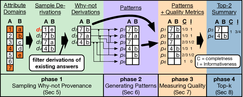
Figure 3: Overview of why-not provenance summarization

4 Overview

Before describing our approach in detail in the following sections, we first give a brief overview. To compute a top-$k$ provenance summary $\mathcal{S}(Q,D,\Phi,k)$ for a provenance question $\Phi$, we have to (i) compute $\textsc{Prov}(\Phi)$, (ii) enumerate all patterns that could be used in summaries, (iii) calculate matches between derivations and the patterns to calculate the completeness of sets of patterns, and (iv) find a set of up to $k$ patterns for $\Phi$ that has the highest score among all such sets of patterns. To compute the exact solution to this problem, we would need to enumerate all derivations from $\textsc{Prov}(\Phi)$. However, this is not feasible for why-not provenance questions since, as we will discuss in the following, the size of why-not provenance $\textsc{Whynot}(Q,D,\bm{t})$ is in $O({\left|{\mathbb{D}}\right|^{n}})$, i.e., linear in the size of the data domain $\mathbb{D}$, but exponential in $n$, the maximal number of variables of a rule from query $Q$ that is not bound to constants by $\bm{t}\in\Phi$. Instead, we present a heuristic approach that uses sampling and outsources most of the computation to a database for scalability. Fig. 3 shows an overview of this approach.

Sampling Provenance (Phase 1, Sec. 5). As shown in Fig. 3 (phase 1), we develop a technique to compute a sample S of $n_{\textsc{S}}$ derivations from $\textsc{Whynot}(Q,D,\bm{t})$ that is unbiased with high probability. We create S by (i) randomly sampling a number of $n_{\textsc{OS}}>n_{\textsc{S}}$ values from the domain of each attribute (e.g., A and B in Fig. 3) individually, (ii) zip these samples to create derivations, and (iii) remove derivations for existing results (e.g., the derivation $d_{1}$ highlighted in red) to compute a sample of $\textsc{Whynot}(Q,D,\bm{t})$ that with high probability is at least of size $n_{\textsc{S}}$ (in Fig. 3 we assumed $n_{\textsc{S}}=3$). For why-provenance, we sample directly from the full provenance for $\Phi$ computed using our query instrumentation technique from [20, 18].

Enumerating Pattern Candidates (Phase 2, Sec. 6). The number of patterns for a rule with $m$ goals and $n$ variables is in $O(\left|{\mathbb{D}+n}\right|^{n}\cdot 2^{m})$. Even if we only consider patterns that match at least one derivation from S, the number of patterns may still be a factor of $2^{n}$ larger than S. We adopt a heuristic from [8] that, in the worst case, generates quadratically many patterns (in the size of S). As shown in Fig. 3, we generate a pattern $p$ for each pair of derivations $d$ and $d^{\prime}$ from S. If $d[i]=d^{\prime}[i]$ then $p[i]=d[i]$. Otherwise $p[i]$ is a fresh placeholder (shown as an empty box in Fig. 3).

Estimating Pattern Coverage (Phase 3, Sec. 7). To be able to compute the completeness metric of a pattern set which is required for scoring pattern sets in the last step, we need to determine what derivations are covered by which pattern and which of these belong to $\textsc{Whynot}(Q,D,\bm{t})$. We estimate completeness based on S. The informativeness of a pattern can be directly computed from the pattern.

Computing the Top-$k$ Summary (Phase 4, Sec. 8). In the last step (phase 4 in Fig. 3), we generate sets of up to $k$ patterns from the set of patterns produced in the previous step, rank them based on their scores, and return the set with the highest score as the top-$k$ summary. We apply a heuristic best-first search method that utilizes efficiently computable bounds for the completeness of sets of patterns to prune the search space.

Query: $r_{ex}:\,\mathtt{Q_{ex}}(X,Y)\,\mathtt{{:}-}\,\mathtt{R}(X,Z),\mathtt{R}(Z,Y),X<Y$

PQ: $\Phi_{ex}=(\bm{t}_{ex},\textsc{Whynot})$ where $\bm{t}_{ex}=\mathtt{Q_{ex}}(X,\textsf{4})$

Query Unified With P-Tuple $\bm{t}_{ex}$:

$$\,\,\,\,\,\,\,\,\,\,\,\,\,\,\,r_{\bm{t}_{ex}}:\,\mathtt{Q_{\bm{t}_{ex}}}(X,4)\,\mathtt{{:}-}\,\mathtt{R}(X,Z),\mathtt{R}(Z,4),X<4$$

R
A	B
1	2
2	3
2	4
5	3
5	5
5	6

$\textbf{Q}_{ex}$
A	B
1	3
1	4
5	6

Answers matching $\bm{t}_{ex}$
A B 1 4 2 4 3 4

Figure 4: Running example for summarization

5 Sampling Why-not Provenance

In this section, we first discuss how to efficiently generate a sample S of annotated derivations of a given size $n_{\textsc{S}}$ from the why-not provenance $\textsc{Whynot}(Q,D,\bm{t})$ for a provenance question (PQ) $\Phi$ (phase 1 in Fig. 3). This sample will then be used in the following phases of our summarization algorithm. We introduce a running example in Fig. 4 and use it through-out Sec. 5 to Sec. 8. Consider the example query $r_{ex}$ shown on the top of Fig. 4 which returns start- and end-points of paths of length 2 in a graph with integer node labels such that the end-point is labeled with a lareger number than the start-point. Evaluating $r_{ex}$ over the example instance $\mathtt{R}$ from the same figure yields three results: $\mathtt{Q_{ex}}(1,3)$, $\mathtt{Q_{ex}}(1,4)$, and $\mathtt{Q_{ex}}(5,6)$. In this example, we want to explain missing answers of the form $\mathtt{Q_{ex}}(X,4)$, i.e., answering the PQ $\Phi_{ex}$ from Fig. 4. Recall that, $\textsc{Whynot}(Q,D,\bm{t})$ for p-tuple $\bm{t}$ consists of all derivations of tuples $t\not\in Q(D)$ where $t\curlyeqprec\bm{t}$. Assuming $\mathbb{D}=\{1,2,3,4,5,6\}$, on the bottom right of Fig. 4 we show all missing and existing answers matching $\bm{t}_{ex}$ (missing answers are shown with red background).

5.1 Naive Unbiased Sampling

To generate all derivations for missing answers, we can bind the variables of each rule $r$ of a query $Q$ to the constants from $\bm{t}$ to ensure that only derivations of results which match the PQ’s p-tuple $\bm{t}$ are generated. We refer to this process as unifying $Q$ with $\bm{t}$. For our running example, this yields the rule $r_{\bm{t}_{ex}}$ shown in Fig. 4. The naive way to create a sample of derivations from $\textsc{Whynot}(Q,D,\bm{t})$ using this rule is to repeatably sample a value from $\mathbb{D}$ for each variable, then check whether (i) the predicates of the rule are fulfilled and (ii) the resulting rule derivation computes a missing answer. For example, for $r_{\bm{t}_{ex}}$, we may choose $X=2$ and $Z=2$ and get a derivation $d_{1}=r_{\bm{t}_{ex}}(2,2)$. The derivation $d_{1}$ fulfills the predicate $X<4$ and its head $\mathtt{Q_{ex}}(2,4)$ is a missing answer. Thus, $d_{1}$ belongs to the why-not provenance of $\bm{t}_{ex}$. Then, to get an annotated rule derivation, we determine its goal annotations by checking whether the tuples corresponding to the grounded goals of the rule exists in the database instance. For this example, $d_{1}=r_{\bm{t}_{ex}}(2,2)-({\color[rgb]{0.8,0,0}F},{\color[rgb]{0,0.45,0}T})$ since the first goal $\mathtt{R}(2,2)$ fails, but the second goal $\mathtt{R}(2,4)$ succeeds. There are two ways of how this process can fail to produce a derivation of $\textsc{Whynot}(Q,D,\bm{t})$: (i) a predicate of the rule may be violated by the bindings generated in this way (e.g., if we would have chosen $X=5$, then $X<4$ would not have held) and (ii) the derivation may derive an existing answer, e.g., if $X=1$ and $Z=3$, we get the failed derivation $r_{\bm{t}_{ex}}(1,3)$ of the existing answer $\mathtt{Q_{ex}}(1,4)$.

Analysis of Naive Sampling. If we repeat the process described above until it has returned $n_{\textsc{S}}$ failed derivations, then this produces an unbiased sample of $\textsc{Whynot}(Q,D,\bm{t})$. Note that, technically, there is no guarantee that the process will ever terminate since it may repeatedly produce derivations that do not fulfill a predicate or derive existing answers. Observe that, typically the amount of missing answers is significantly larger than the number of answers, i.e., $\left|{\textsc{Whynot}(Q,D,\bm{t})}\right|\gg\left|{\mathcal{A}(Q,D,\bm{t})-\textsc{Whynot}(Q,D,\bm{t})}\right|$. As a result, any randomly generated derivation is with high probability in $\textsc{Whynot}(Q,D,\bm{t})$. We will explain how to deal with derivations that fail to fulfill predicates in Sec. 5.2.

Batch Sampling. A major shortcoming of the naive sampling approach is that it requires us to evaluate queries to test for every produced derivation $d$ whether it derives a missing answer ( $\mathsf{head}(d)\not\in Q(D)$) and to determine its goal annotations by checking for each grounded goal $R(\vec{c})$ or $\neg R(\vec{c})$ whether $R(\vec{c})\in D$. It would be more efficient to model sampling as a single batch computation that we can outsource to a database system and that can be fused into a single query with the other phases of the summarization process to avoid unnecessary round-trips between our system and the database. However, for batch sampling, we have to choose upfront how many samples to create, but not all such samples will end up being why-not provenance or fulfill the rule’s predicates. To ensure with high probability that the batch computation returns at least $n_{\textsc{S}}$ derivations from $\textsc{Whynot}(Q,D,\bm{t})$, we use a larger sample size $n_{\textsc{OS}}\geq n_{\textsc{S}}$ such that the probability that the resulting sample contains at least $n_{\textsc{S}}$ derivations from $\textsc{Whynot}(Q,D,\bm{t})$ is higher than a configurable threshold $P_{success}$ (e.g., 99.9%). We refer to this part of the process as over-sampling. We discuss how to generate a query that computes a sample of size $n_{\textsc{OS}}$ in Sec. 5.2 and, then, discuss how to determine $n_{\textsc{OS}}$ in Sec. 5.3.

inline,color=green!60]Deleted for revision: we introduced an approach which instruments an input Datalog program to out-source provenance computation to a database system. Challenge 1. As mentioned in Section Sec. 1, the number of derivations in $\textsc{Whynot}(Q,D,\bm{t})$ is in the order of $O({\left|{\mathbb{D}}\right|^{n}})$ where $n$ is the maximal number of variables in a rule of $Q$ excluding variables bound to constants by $\bm{t}$ (we call these unbound variables). Thus, it is not feasible to enumerate all derivations in $\textsc{Whynot}(Q,D,\bm{t})$ during summarization. To develop a batch sampling method we have to overcome several challenges: (i) how to express sampling using queries and (ii) how to determine $n_{\textsc{OS}}$, the number of derivations that the process should produce such that the chance of getting a sample with at least $n_{\textsc{S}}$ derivation from the why-not provenance is larger than a configurable success probability $P_{success}$. We present our solution for the first challenge in Sec. 5.2 and discuss how to determine $n_{\textsc{OS}}$ in Sec. 5.3.

5.2 Batch Sampling Using Queries

inline,color=green!60]Deleted for revision:Our batch sampling technique is based on the following observations: (i) we can partition the set of derivations for tuples matching $\bm{t}$ from $\Phi$ into derivations for existing and missing tuples. The second partition is $\textsc{Whynot}(Q,D,\bm{t})$. Ignoring the goal annotations for now, for any derivation $d\in\mathcal{A}(Q,D,\bm{t})$ that derives a tuple $t\curlyeqprec\bm{t}$ we can decide its membership in $\textsc{Whynot}(Q,D,\bm{t})$ by checking whether $t\not\in Q(D)$ (using the original query result only); (ii) typically $\left|{\textsc{Whynot}(Q,D,\bm{t})}\right|\gg\left|{\mathcal{A}(Q,D,\bm{t})-\textsc{Whynot}(Q,D,\bm{t})}\right|$ and, thus, any randomly generated derivation for some $t\curlyeqprec\bm{t}$ is with high probability in $\textsc{Whynot}(Q,D,\bm{t})$; and (iii) given a derivation $d$ without goal annotations, we can determine the goal annotations by checking for each grounded goal $R(\vec{c})$ or $\neg R(\vec{c})$ whether $R(\vec{c})\in D$. Based on these observations, we devise the algorithm that generates S of size $n_{\textsc{S}}$.

For simplicity, we limit the discussion to queries with a single rule, e.g., the query $r_{ex}$ from Fig. 4. We discuss queries with multiple rules at the end of this section. The query we generate to produce a sample of size $n_{\textsc{OS}}$ consists of three steps: generating derivations, filtering derivations of existing answers, determining goal annotations.

1. Generating Derivations. We first generate a query that creates a random sample OS of $n_{\textsc{OS}}$ derivations (not annotated) for which there exists an annotated version in $\mathcal{A}(Q,D,\bm{t})$ (all annotated derivations that match head $Q(\bm{t})$). Consider a single rule $r$ with $m$ literal goals, $n$ variables, and $h$ head variables: $r:\mathtt{Q}(\overline{{X}})\,\mathtt{{:}-}\,\mathtt{g_{1}}(\overline{{X_{1}}}),\ldots,\mathtt{g_{m}}(\overline{{X_{m}}}),$ $\psi_{1}(\overline{{Y_{1}}}),$ $\ldots,\psi_{k}(\overline{{Y_{l}}})$. Let $R_{i}$ be the relation accessed by goal $\mathtt{g_{i}}$, i.e., $\mathtt{g_{i}}(\overline{{X_{i}}})$ is either $R_{i}(\overline{{X_{i}}})$ or $\neg R_{i}(\overline{{X_{i}}})$. color=red!40,inline]Boris says:For now, we assume that the rule does not contain predicates (how we deal with predicates will be discussed later). Let $k$ be the number of head variables bound by the p-tuple $\bm{t}$ from the question $\Phi$ for which we are sampling. We use $\overline{{Z}}=Z_{1},\ldots,Z_{u}$ to denote the $u=n-k$ variables of $r$ that are not bound by $\bm{t}$. Recall that, to only consider derivations matching $\bm{t}$, we unify the rule with $\bm{t}$ by binding variables in the rule to the corresponding constants from $\bm{t}$. We use $r_{\bm{t}}$ to denote the resulting unified rule. Note that we will describe our summarization techniques using derivations and patterns for $r_{\bm{t}}$. Patterns for $r$ can be trivially reconstructed from the results of summarization by plugging in constants from $\bm{t}$. To generate derivations for such a query, we sample $n_{\textsc{OS}}$ values for each unbound variable independently with replacement, and, then, combine the resulting samples into a sample of $\mathcal{A}(Q,D,\bm{t})$ modulo goal annotations. Predicates comparing constants with variables, e.g., $X<4$ in $r_{\bm{t}_{ex}}$, are applied before sampling to remove values from the domain of a variable that cannot result in derivations fulfilling the predicates. Similar to [20, 18], we assume that the user specifies the domain $\mathbb{D}_{A}$ for each attribute $A$ as a unary query that returns $\mathbb{D}_{A}$ (we provide reasonable defaults to avoid overloading the user). We extend the relational algebra with two operators to be able to express sampling. Operator $\textsc{Sample}_{n}$ returns $n$ samples which are chosen uniformly random with replacement from the input of the operator. We use $\#_{A}$ to denote an operator that creates an integer identifier for each input row that is stored in a column $A$ appended to the schema of the operator’s input. For each variable $X\in\overline{{Z}}$ with $\mathsf{attrs}(X)=\{A_{1},\ldots,A_{j}\}$ ($\mathsf{attrs}(X)$ denotes the set of attributes that variable $X$ is bound to by the rule containing $X$), we create a query $Q_{X}$ that unions the domains of these attributes, then applies predicates that compare $X$ with constants, and then samples $n_{\textsc{OS}}$ values.

$$Q_{X}\coloneqq\#_{id}(\textsc{Sample}_{n_{\textsc{OS}}}(\sigma_{\theta_{X}}(\rho_{X}((\mathbb{D}_{A_{1}}\cup\ldots\cup\mathbb{D}_{A_{j}}))))$$

Here, $\theta_{X}$ is a conjunction of all the predicates from $r_{\bm{t}}$ that compare $X$ with a constant. The purpose of $\#$ is to allow us to use natural join to “zip” the samples for the individual variables into bindings for all variables of $r_{\bm{t}}$:

$$Q_{bind}\coloneqq\sigma_{\theta_{join}}(Q_{Z_{1}}\bowtie\ldots\bowtie Q_{Z_{u}})$$

Here, $\theta_{join}$ is a conjunction of all predicates from $r_{\bm{t}}$ that compare two variables. Note that the selectivity of $\theta_{join}$ has to be taken into account when computing $n_{\textsc{OS}}$ (discussed in Sec. 5.3). Each tuple in the result of $Q_{bind}$ encodes the bindings for one derivation $d$ of a tuple $t\curlyeqprec\bm{t}$.

Example 4

Consider unified rule $r_{\bm{t}_{ex}}$ from Fig. 4. Assume that $\mathbb{D}_{A}=\mathbb{D}_{B}=\Pi_{A}(R)\cup\Pi_{B}(R)$ and $n_{\textsc{OS}}=3$. Variable $X$ is bound to attribute $A$ and $Z$ is bound to both $A$ and $B$. Thus, we generate the following queries:

$$Q_{X} \coloneqq\#_{id}(\textsc{Sample}_{n_{\textsc{OS}}}(\sigma_{X<4}(\rho_{X}(\mathbb{D}_{A}))))$$

$$Q_{Z} \coloneqq\#_{id}(\textsc{Sample}_{n_{\textsc{OS}}}(\rho_{Z}(\mathbb{D}_{A}\cup\mathbb{D}_{B})))$$

$$Q_{bind} \coloneqq\sigma_{true}(Q_{X}\bowtie Q_{Z})$$

Evaluated over the example instance, this query may return:

$Q_{X}$ id X 1 1 2 2 3 2

$Q_{Z}$ id Z 1 4 2 2 3 4

$Q_{bind}$ id X Z 1 1 4 2 2 2 3 2 4

2. Filtering Derivations of Existing Answers. We now construct a query $Q_{der}$, which checks for each derivation $d\in\textsc{OS}$ for a tuple $t\curlyeqprec\bm{t}$ whether $t\not\in Q(D)$ and only retain derivations passing this check. This is achieved by anti-joining ($\vartriangleright$) $Q_{bind}$ with $Q$ which we restricted to tuples matching $\bm{t}$ since only such tuples can be derived by $Q_{bind}$.

$$Q_{der}\coloneqq Q_{bind}\vartriangleright_{\theta_{der}}\sigma_{\theta_{\bm{t}}}(Q)$$

The query $Q_{der}$ uses condition $\theta_{der}$ which equates attributes from $Q_{bind}$ that correspond to head variables of $r_{\bm{t}}$ with the corresponding attribute from $Q$ and condition $\theta_{\bm{t}}$ that filters out derivations not matching $\bm{t}$ by equating attributes with constants from $\bm{t}$.

Example 5

From $Q_{ex}$ in Fig. 4, we remove answers where $Y\neq 4$ (since $\bm{t}_{ex}$ binds $Y=4$) and anti-join on $X$, the only head variable of $r_{\bm{t}_{ex}}$, with $Q_{bind}$ from Ex. 4. The resulting query and its result are shown below. Note that tuple $(1,1,4)$ was removed since it corresponds to a (failed) derivation of the existing answer $\mathtt{Q_{ex}}(1,4)$.

$$Q_{der}\coloneqq Q_{bind}\vartriangleright_{X=X}\sigma_{Y=4}(Q_{ex})$$

id	X	Z
2	2	2
3	2	4

3. Computing Goal Annotations. Next, we determine goal annotations for each derivation to create a set of annotated derivations from $\textsc{Whynot}(Q,D,\bm{t})$. Recall that a positive (negative) grounded goal is successful if the corresponding tuple exists (is missing). We can check this by outer-joining the derivations with the relations from the rule’s body. Based on the existence of a join partner, we create boolean attributes storing $g_{i}$ for $1\leq i\leq|\mathsf{body}(r)|$ (${\color[rgb]{0.8,0,0}F}$ is encoded as false). For a negated goal, we negate the result of the conditional expression such that ${\color[rgb]{0.8,0,0}F}$ is used if a join partner exists. We construct query $Q_{sample}$ shown below to associates derivations in $Q_{der}$ with the goal annotations $\bar{g}$.

$$Q_{sample} \coloneqq\delta(\Pi_{Z_{1},\cdots,Z_{u},e_{1}\to g_{1},\cdots,e_{n}\to g_{m}}(Q_{goals}))$$

$$Q_{goals}\coloneqq Q_{der}\mathbin{\rule[-0.08612pt]{2.5pt}{0.4pt}\hbox to0.0pt{\hss\rule[7.0pt]{2.5pt}{0.4pt}}\mkern-5.8mu\bowtie}_{\theta_{1}}\Pi_{\mathbf{R_{1}},1\to h_{1}}(\mathtt{R_{1}})\ldots\mathbin{\rule[-0.08612pt]{2.5pt}{0.4pt}\hbox to0.0pt{\hss\rule[7.0pt]{2.5pt}{0.4pt}}\mkern-5.8mu\bowtie}_{\theta_{n}}\Pi_{\mathbf{R_{1}},1\to h_{m}}(\mathtt{R_{m}})$$

Note that we use duplicate elimination to preserve set semantics. In projection expressions, we use $e\to a$ to denote projection on a scalar expression $e$ whose result is stored in attribute $a$. Here, the join condition $\theta_{i}$ equates the attributes storing the values from $\overline{{X_{i}}}$ in $r_{\bm{t}}$ with the corresponding attributes from $R_{i}$. Attributes at positions that are bound to constants in $r_{\bm{t}}$ are equated with the constant. The net effect is that a tuple from $Q_{der}$ corresponding to a rule derivation $d$ has a join partner in $R_{i}$ iff the tuple corresponding to the $i^{th}$ goal of $d$ exists in $D$. The expression $e_{i}$ used in the projection of $Q_{sample}$ then computes the boolean indicator for goal $g_{i}$ as follows:

$$e_{i}\coloneqq\begin{cases}\text{\bf if}\thickspace(\mathbf{isnull}(h_{i}))\thickspace\text{\bf then}\thickspace{\color[rgb]{0.8,0,0}F}\thickspace\text{\bf else}\thickspace{\color[rgb]{0,0.45,0}T}&\text{if}\,g_{i}\,\text{is positive}\\ \text{\bf if}\thickspace(\mathbf{isnull}(h_{i}))\thickspace\text{\bf then}\thickspace{\color[rgb]{0,0.45,0}T}\thickspace\text{\bf else}\thickspace{\color[rgb]{0.8,0,0}F}&\text{otherwise}\end{cases}$$

Example 6

For our running example, we generate:

$$Q_{sample} \coloneqq\delta(\Pi_{\begin{subarray}{c}X,Z,\text{\bf if}\thickspace(\mathbf{isnull}(h_{1}))\thickspace\text{\bf then}\thickspace{\color[rgb]{0.8,0,0}F}\thickspace\text{\bf else}\thickspace{\color[rgb]{0,0.45,0}T}\to g_{1},\\ \text{\bf if}\thickspace(\mathbf{isnull}(h_{2}))\thickspace\text{\bf then}\thickspace{\color[rgb]{0.8,0,0}F}\thickspace\text{\bf else}\thickspace{\color[rgb]{0,0.45,0}T}\to g_{2}\end{subarray}}(Q_{goals}))$$

$$Q_{goals} \coloneqq Q_{der}\mathbin{\rule[-0.08612pt]{2.5pt}{0.4pt}\hbox to0.0pt{\hss\rule[7.0pt]{2.5pt}{0.4pt}}\mkern-5.8mu\bowtie}_{X=A\wedge Z=B}\Pi_{A,B,1\to h_{1}}(R)$$

$$\hskip 14.22636pt\mathbin{\rule[-0.08612pt]{2.5pt}{0.4pt}\hbox to0.0pt{\hss\rule[7.0pt]{2.5pt}{0.4pt}}\mkern-5.8mu\bowtie}_{Z=A\wedge B=4}\Pi_{A,B,1\to h_{2}}(R)$$

Evaluating this query, we get the result shown below.

$Q_{sample}$ id X Z $h_{1}$ $h_{2}$ 2 2 2 F T 3 2 4 T F

The first tuple corresponds to the derivation $r_{\bm{t}_{ex}}(2,2)-({\color[rgb]{0.8,0,0}F},{\color[rgb]{0,0.45,0}T})$ for which the first goal fails since $\mathtt{R}(2,2)$ does not exist in $\mathtt{R}$ while the second goal succeeds because $\mathtt{R}(2,4)$ exists. Similarly, the second tuple corresponds to $r_{\bm{t}_{ex}}(2,4)-({\color[rgb]{0,0.45,0}T},{\color[rgb]{0.8,0,0}F})$ for which the first goal succeeds since $\mathtt{R}(2,4)$ exists while the second goal fails because $\mathtt{R}(4,4)$ does not exist.

color=red!40,inline]Boris says:remove overlapping parts, and move what remains to Sec 5.2

Queries With Multiple Rules. For queries with multiple rules, we determine $n_{\textsc{OS}}$ separately for each rule (recall that we consider $\mathsf{UCQ}^{\neg<}$ queries where every rule has the same head predicate) and create a separate query for each rule as described above. Patterns are also generated separately for each rule. In the final step, we then select the top-$k$ summary from the union of the sets of patterns. inline,color=green!60]Deleted for revision:For simplicity, Algorithm LABEL:alg:sampling shows pseudocode for a variant of our sampling algorithm which directly computes a sample without constructing a query that computes the sample.

Complexity. The runtime of our algorithm is linear in $n_{\textsc{OS}}$ and $\left|{D}\right|$ which significantly improves over the naive algorithm which is in $O({|\mathbb{D}|^{n}})$.

Implementation. Some DBMS such as Oracle and Postgres support a sample operator out of the box which we can use to implement the Sample operator introduced above. However, these implementations of a sampling operator do not support sampling with replacement out of the box. We can achieve decent performance for sampling with replacement using a set-returning function that takes as input the result of applying the built-in sampling operator to generate a sample of size $n_{\textsc{OS}}$, caches this sample, and then samples $n_{\textsc{OS}}$ times from the cached sample with replacement. The $\#_{A}$ operator can be implemented in SQL using ROW_NUMBER(). The expressions $\text{\bf if}\thickspace(\theta)\thickspace\text{\bf then}\thickspace e_{1}\thickspace\text{\bf else}\thickspace e_{2}$ and $\mathbf{isnull}($) can be expressed in SQL using CASE WHEN and IS NULL, respectively.

5.3 Determining Over-sampling Size

We now discuss how to choose $n_{\textsc{OS}}$, the size of the sample OS produced by query $Q_{bind}$, such that the probability that OS contains at least $n_{\textsc{S}}$ derivations from $\textsc{Whynot}(Q,D,\bm{t})$ is higher than a threshold $P_{success}$ under the assumption that the sampling method we introduced above samples uniformly random from $\mathcal{A}(Q,D,\bm{t})$. We, then, prove that our sampling method returns a uniform random sample. First, consider the probability $p_{prov}$ that a derivation chosen uniformly random from $\mathcal{A}(Q,D,\bm{t})$ is in $\textsc{Whynot}(Q,D,\bm{t})$ which is equal to the faction of derivations from $\mathcal{A}(Q,D,\bm{t})$ that are in $\textsc{Whynot}(Q,D,\bm{t})$:
$$p_{prov}=\frac{\left|{\textsc{Whynot}(Q,D,\bm{t})}\right|}{\left|{\mathcal{A}(Q,D,\bm{t})}\right|}$$

$\left|{\mathcal{A}(Q,D,\bm{t})}\right|$ can be computed from $Q$, $\bm{t}$, and the attribute domains as explained in Sec. 2.2. For instance, consider $\mathbb{D}=\{1,2,3,4,5,6\}$ as the universal domain and rule $r_{\bm{t}_{ex}}$ from our running example, but without the conditional predicate. Then, there are $\left|{\mathbb{D}}\right|^{n}=6^{2}$ possible derivations of this rule because neither variable $X$ nor $Z$ are not bound by $\bm{t}_{ex}$ and $\mathbb{D}$ has 6 values. To determine $\left|{\textsc{Whynot}(Q,D,\bm{t})}\right|$, we need to know how many derivations in $\mathcal{A}(Q,D,\bm{t})$ correspond to missing tuples matching $\bm{t}$. Since in most cases the number of missing answers is significantly larger than the number of existing tuples, it is more effective to compute the number of (successful and/or failed) derivations of $t\in Q(D)$ with $t\curlyeqprec\bm{t}$, i.e., $\left|{\{t\mid t\in Q(D)\wedge t\curlyeqprec\bm{t}\}}\right|$. This gives us the probability $p_{notProv}$ that a derivation is not in $\textsc{Whynot}(Q,D,\bm{t})$ and we get: $p_{prov}=1-p_{notProv}$.

Next, consider a random variable $X$ that is the number of derivations from $\textsc{Whynot}(Q,D,\bm{t})$ in OS. We want to compute the probability $p(X\geq n_{\textsc{S}})$. For that, consider first $p(X=i)$, the probability that the sample OS we produce contains exactly $i$ derivations from $\textsc{Whynot}(Q,D,\bm{t})$. We can apply standard results from statistics for computing $p(X=i)$, i.e., out of a sequence of $n_{\textsc{OS}}$ picks with probability $p_{prov}$ we get $i$ successes. The probability to get exactly $i$ successes out of $n$ picks is $\binom{n}{i}\cdot{p_{prov}}^{i}\cdot(1-p_{prov})^{n-i}$ based on the Binomial Distribution. For $i\neq j$, the events $X=i$ and $X=j$ are disjoint (it is impossible to have both exactly $i$ and $j$ derivations from $\textsc{Whynot}(Q,D,\bm{t})$ in OS). Thus, $p(X\geq n_{\textsc{S}})$ is $\sum p(X=i)$ for $i\in\{n_{\textsc{S}},\ldots,n_{\textsc{OS}}\}$:

$$p(X\geq n_{\textsc{S}})=\sum_{i=n_{\textsc{S}}}^{n_{\textsc{OS}}}\binom{n_{\textsc{OS}}}{i}\cdot{p_{prov}}^{i}\cdot(1-p_{prov})^{n_{\textsc{OS}}-i}$$

Given $p_{prov}$, $n_{\textsc{S}}$, and $P_{success}$, we can compute the sample size $n_{\textsc{OS}}$ such that $p(X\geq n_{\textsc{S}})$ is larger than $P_{success}$ ([1, 28] presents an algorithm for finding the minimum such $n_{\textsc{OS}}$). color=red!40,inline]Boris says:This is now out of place: remove or merge into beginning In the following subsections, we explain how to optimize the remaining summarization process further utilizing a sample S generated over our technique, i.e., using S for generating candidate patterns (Section LABEL:sec:opt-patgen) and measuring quality of patterns (Section LABEL:sec:approx-summ).

Handling Predicates. Recall that we apply predicates that compare a variable with a constant before creating a sample for this variable. Thus, we do not need to consider these predicates when determining $n_{\textsc{OS}}$. Predicates comparing variables with variables are applied after the step of creating derivations. We estimate the selectivity of such predicates using standard techniques [15] to estimate how many derivations will be filtered out and, then, increase $n_{\textsc{OS}}$ to compensate for this, e.g., for a predicate with $0.5$ selectivity we would double $n_{\textsc{OS}}$.

5.4 Analysis of Sampling Bias

We now formally analyze if our approach creates a uniform sample of $\textsc{Whynot}(Q,D,\bm{t})$. We demonstrate this by analyzing the probability $p(d\in\textsc{S})$ for an arbitrary derivation $d\in\textsc{Whynot}(Q,D,\bm{t})$ to be in the sample S. If our approach is unbiased, then this probability should be independent of which $d$ is chosen and for $d^{\prime}\neq d$ the events $d\in\textsc{S}$ and $d^{\prime}\in\textsc{S}$ should be independent.

Theorem 1

Given derivations $d,d^{\prime}\in\textsc{Whynot}(Q,D,\bm{t})$ and sample sizes $n_{\textsc{S}}$ and $n_{\textsc{OS}}$, $p(d\in\textsc{S})=c$ where $c$ is a constant that is independent of the choice of $d$. Furthermore, the events $d\in\textsc{S}$ and $d^{\prime}\in\textsc{S}$ are independent of each other.

Proof 5.1.

To prove the theorem, we have to demonstrate that none of the phases of sampling introduces bias. In the following, let $\mathcal{A}\coloneqq\mathcal{A}(Q,D,\bm{t})$, $n_{A}\coloneqq\left|{\mathcal{A}}\right|$, and $n_{P}\coloneqq\left|{\mathcal{P}}\right|$ where $\mathcal{P}\coloneqq\textsc{Whynot}(Q,D,\bm{t})$. Recall that the first phase of sampling generates a sample OS of size $n_{\textsc{OS}}$ by independently creating samples for each unbound variable which are combined into a sample of $\mathcal{A}$. Consider first the case where $n_{\textsc{OS}}=1$, i.e., we pick a single value from each domain. Let $\mathbb{D}_{i}$ denote the domain for unbound variable $Z_{i}$ in the single rule $r$ of query $Q$. Since we sample uniform from $\mathbb{D}_{i}$, each of the $\left|{\mathbb{D}_{i}}\right|$ values has a probability of $\frac{1}{\left|{\mathbb{D}_{i}}\right|}$ to be chosen. Since the sample for $Z_{i}$ is chosen independently from $Z_{j}$ for $i\neq j$, any particular derivation $d\in\mathcal{A}$ to be in OS is . For $n_{\textsc{OS}}>1$, observe that each value in the sample of $\mathbb{D}_{i}$ is chosen independently. Thus, (the last equivalence is based on when $A$ and $B$ are independent). Furthermore, this implies that $d\in\textsc{OS}$ is independent of $d^{\prime}\in\textsc{OS}$ for $d\neq d^{\prime}$. So far, we have established that is constant and the events for picking particular derivations are mutually independent. It remains to be shown that the same holds for a derivation $d\in\mathcal{P}$ and the sample S we derive from OS. Since OS is sampled from $\mathcal{A}$, it may contain derivations $d^{\prime}\not\in\mathcal{P}$. Our sampling algorithms filters such derivations. Let $\textsc{S}_{np}$ denote the set of all such derivations from OS and $n_{np}=\left|{\textsc{S}_{np}}\right|$. Observe that for $i\neq j$ the events $n_{np}=i$ and $n_{np}=j$ are obviously disjoint since OS contains a fixed number of derivations not in $\mathcal{P}$. Furthermore, $\sum_{i=0}^{n_{\textsc{OS}}}$ since OS has to contain anywhere from zero to $n_{\textsc{OS}}$ such derivations. Thus, we can compute the probability as the sum over $i=\{0,\ldots,n_{\textsc{OS}}\}$ of the probability that $d$ is selected to be in S conditioned on the probability that $d\in\textsc{OS}$ (otherwise $d$ cannot be in S) and that $n_{np}=i$.

$$\thickspace\thickspace\thickspace\thickspace\thickspace\thickspace\sum_{i=0}^{n_{\textsc{OS}}}$$

Now, consider the individual probabilities in this formula. Let $p_{1}=$. If $d$ is in OS and $n_{np}=i$, then there are $n_{\textsc{OS}}-i-1$ derivations from $\mathcal{P}$ in OS. Our sampling algorithm selects uniformly $n_{\textsc{S}}$ derivation in $\mathcal{P}$ from $\textsc{OS}-\textsc{S}_{np}$ if $n_{\textsc{OS}}-i>n_{\textsc{S}}$. Thus, the probability for our particular derivation $d$ to be in the final result is:

$$p_{1}=\frac{\min(n_{\textsc{S}},n_{\textsc{OS}}-i)}{n_{\textsc{OS}}-i}$$

Next, consider $p_{2}=$. Based on our observation above, any subset of derivations of $\mathcal{A}$ has the same probability to be returned as OS. Thus, $p_{2}$ can be computed as the fraction of subsets of $\mathcal{A}$ of size $n_{\textsc{OS}}$ that contain $i$ successful derivation(s), and $d$ and $n_{\textsc{OS}}-i-1$ other derivations from $\mathcal{P}$. Putting differently, how many of the ${n_{A}}^{n_{\textsc{OS}}}$ possible samples that could be produced by our algorithm contain $d$ and exactly $i$ derivations from $\textsc{S}_{np}$:

$$p_{2}=\frac{{n_{np}}^{i}\cdot{n_{P}}^{n_{\textsc{OS}}-i-1}}{{n_{A}}^{n_{\textsc{OS}}}}$$

Observe, that the formulas for $p_{1}$ and $p_{2}$ only refer to constants that are independent of the choice of $d$. Thus, is independent of the choice of $d$.

6 Generating Pattern Candidates

We now explain the candidate generation step of our summarization approach (phase 2 in Fig. 3). Consider a provenance question (PQ) $\Phi=(\bm{t},\textsc{Whynot})$ for a query $Q$. For any rule $r$ of $Q$, let $n$ be the number of unbound variables, i.e., $\left|{\mathsf{vars}(r_{\bm{t}})}\right|$ where $r_{\bm{t}}$ is the unified rule for $r$ and $\bm{t}$, and $m$ be the number of goals in $r$. The number of possible patterns for $r_{\bm{t}}$ is in $O({(\left|{\mathbb{D}}\right|+n)^{n}\cdot 2^{m}})$, because for each variable of $r_{\bm{t}}$ we can choose either a placeholder or a value from $\mathbb{D}$ and for each goal we have to pick one of two possible annotations (${\color[rgb]{0.8,0,0}F}$ or ${\color[rgb]{0,0.45,0}T}$). Note that the names of placeholders are irrelevant to the semantics of a pattern, e.g., patterns $p=(A,3)$ and $p^{\prime}=(B,3)$ are equivalent (matching the same derivations). That is, we only have to decide which arguments of a pattern are placeholders and which arguments share the same placeholder. Thus, it is sufficient to only consider $n$ distinct placeholders $P_{i}$ (where $1\leq i\leq n$) when creating patterns for a unified rule $r_{\bm{t}}$ with $n$ variables.

Example 7

Consider rule $r_{\bm{t}_{ex}}$ from Fig. 4. Let $\mathbb{D}=\{1,2,3,4,5,6\}$ and $\mathbb{P}=\{P_{1},P_{2}\}$. Let us for now ignore goal annotations. Note that, taking the predicate $X<4$ into account, any pattern where $X\geq 4$ cannot possibly match any derivations for this rules and, thus, we only have to consider patterns where $X$ is bound to a constant less than 4 or a placeholder. The set of viable patterns is:
$\displaystyle r_{\bm{t}_{ex}}(P_{1},P_{2}),r_{\bm{t}_{ex}}(P_{1},1),\ldots,r_{\bm{t}_{ex}}(P_{1},6),r_{\bm{t}_{ex}}(1,P_{2}),\ldots,r_{\bm{t}_{ex}}(6,P_{2}),$ $\displaystyle r_{\bm{t}_{ex}}(1,1),\ldots,r_{\bm{t}_{ex}}(1,6),\ldots r_{\bm{t}_{ex}}(3,1),\ldots,r_{\bm{t}_{ex}}(3,6)$
This set contains $31$ elements. Considering goal annotations $({\color[rgb]{0.8,0,0}F},{\color[rgb]{0.8,0,0}F})$, $({\color[rgb]{0.8,0,0}F},{\color[rgb]{0,0.45,0}T})$, and $({\color[rgb]{0,0.45,0}T},{\color[rgb]{0.8,0,0}F})$, we get $31\cdot 3=93$ patterns.

Given the $O({(\left|{\mathbb{D}}\right|+n)^{n}\cdot 2^{m}})$ complexity, it is not feasible to enumerate all possible patterns. Instead, we adapt the Lowest Common Ancestor (LCA) method [8, 9] for our purpose which generates a number of pattern candidates from the derivations in a sample S that is at most quadratic in $n_{\textsc{S}}$. Thus, this approach sacrifices completeness to achieve better performance. Given a set of derivations (tuples in the work from [8, 9]), the LCA method computes the cross-product of this set with itself and generates candidate explanations by generalizing each such pair. The rationale is that each pattern generated in this fashion will at least match two derivations (or one derivation for the special case where a derivation is paired with itself). In our adaptation, we match derivations on the goal annotations such that only derivations with the same success/failure status of goals are paired. For each pair of derivations $d_{1}=(a_{1},\ldots,a_{n})-(\bar{g})$ and $d_{2}=(b_{1},\ldots,b_{n})-(\bar{g})$, we generate a pattern $p=(c_{1},\ldots,c_{n})-(\bar{g})$. We determine each element $c_{i}$ in $p$ as follows. If $a_{i}=b_{i}$ then $c_{i}=a_{i}$. That is, constants on which $d_{1}$ and $d_{2}$ agree are retained. Otherwise, $c_{i}$ is a fresh placeholder.

Example 8

Reconsider the unified rule $r_{\bm{t}_{ex}}$ and instance $\mathtt{R}$ from Fig. 4. Two example annotated rule derivations are $d_{1}=r_{\bm{t}_{ex}}(2,1)-({\color[rgb]{0.8,0,0}F},{\color[rgb]{0.8,0,0}F})$ and $d_{2}=r_{\bm{t}_{ex}}(2,5)-({\color[rgb]{0.8,0,0}F},{\color[rgb]{0.8,0,0}F})$. LCA generate a pattern $p=r_{\bm{t}_{ex}}(2,Z)-({\color[rgb]{0.8,0,0}F},{\color[rgb]{0.8,0,0}F})$ to generalize $d_{1}$ and $d_{2}$ because $d_{1}[1]=d_{2}[1]=2$ (and, thus, this constant is retained) and ${p}[{2}]=Z$ since $d_{1}[2]=1\neq 5=d_{2}[2]$.

We apply LCA to the sample S created using $Q_{sample}$ from Sec. 5.2. Using LCA, we avoid generating exponentially many patterns and, thus, improve the runtime of pattern generation from $O({\left|{\mathbb{D}}\right|^{n}})$ to $O({{n_{\textsc{S}}}^{2}})$ where typically $n_{\textsc{S}}\ll|\mathbb{D}|$. Furthermore, this optimization reduces the input size for the final stages of the summarization process leading to additional performance improvements. Even though LCA is only a heuristic, we demonstrate experimentally in Sec. 9 that it performs well in practice. inline,color=red!40]Boris deleted:We use $\textsc{Pat}_{lca}(Q,\bm{t})$ to denote pattern candidates generated using LCA for a p-tuple $\bm{t}$.because: Not used

Implementation. We implement the LCA method as a query $Q_{lca}$ joining the query $Q_{sample}$ (the query producing S) with itself on a condition $\theta_{lca}\coloneqq\bigwedge_{i=0}^{m}g_{i}=g_{i}$ where $m$ is the number of goals of the rule $r$ of $Q$ (recall that we create patterns for each rule of $Q$ independently and merge in the final step). Patterns are generated using a projection on an list of expressions $A_{lca}$, where the $i^{th}$ argument of a pattern is determined as $\text{\bf if}\thickspace(X_{i}=X_{i})\thickspace\text{\bf then}\thickspace X_{i}\thickspace\text{\bf else}\thickspace NULL$. Note that the LCA method never generates patterns where the same placeholder appears more than once. Thus, it is sufficient to encode placeholders as NULL values.

$$Q_{lca}\coloneqq\delta(\Pi_{A_{lca}}(Q_{sample}\bowtie_{\theta_{lca}}Q_{sample}))$$

The query generated for our running example is:

$$Q_{lca} \coloneqq\delta(\Pi_{e_{X}\to X,e_{Z}\to Z}(Q_{sample}\bowtie_{(g_{1}=g_{1})\wedge(g_{2}=g_{2})}Q_{sample})$$

$$e_{X} \coloneqq\text{\bf if}\thickspace(X=X)\thickspace\text{\bf then}\thickspace X\thickspace\text{\bf else}\thickspace NULL$$

$$e_{Z} \coloneqq\text{\bf if}\thickspace(Z=Z)\thickspace\text{\bf then}\thickspace Z\thickspace\text{\bf else}\thickspace NULL$$

inline,color=green!60]Deleted for revision:Note that we can replace LCA with any other methods for computing candidate patterns without having to change the other steps of our summarization process. Studying alternative method is an interesting avenue for future work.

7 Estimating Completeness

To generate a top-$k$ summary in the next step, we need to calculate the informativeness (Def. 8) and completeness (Def. 7) quality metrics for sets of patterns. Informativeness can be computed from patterns without accessing the data. Recall that completeness is computed as the fraction of provenance matched by a pattern: $cp(p)=\frac{\left|{\mathcal{M}(Q,D,p,\Phi)}\right|}{\left|{\textsc{Prov}(\Phi)}\right|}$. Since we can materialize neither $\left|{\mathcal{M}(Q,D,p,\Phi)}\right|$ nor $\left|{\textsc{Prov}(\Phi)}\right|$ for the why-not provenance, we have to estimate their sizes. In this section, we focus on how to estimate the completeness of individual patterns. How to compute the completeness metric for sets of patterns will be discussed in Sec. 8.

To determine whether a derivation $d\in\textsc{Prov}(\Phi)$ with goal annotations $\bar{g_{1}}$ matches a pattern $p$ with goal annotations $\bar{g_{2}}$ that is in $\mathcal{M}(Q,D,p,\Phi)$, we have to check that $\bar{g_{1}}=\bar{g_{2}}$ and a valuation exists that maps $p$ to $d$. Then, we count the number of such derivations to compute $\left|{\mathcal{M}(Q,D,p,\Phi)}\right|$. The existence of a valuation can be checked in linear time in the number of arguments of $p$ by fixing a placeholder order and, then, assigning to each placeholder in $p$ the corresponding constant in $d$ if a unique such constant exists. The valuation fails if $p$ and $d$ end up having two different constants at the same position.

Example 9

Continuing with Ex. 8, we compute completeness of the pattern $p=r_{\bm{t}_{ex}}(2,Z)-({\color[rgb]{0.8,0,0}F},{\color[rgb]{0.8,0,0}F})$. For sake of the example, assume that $\textsc{Prov}(\Phi_{ex})=$:
$\displaystyle d_{1}=r_{\bm{t}_{ex}}(2,1)-({\color[rgb]{0.8,0,0}F},{\color[rgb]{0.8,0,0}F})\hskip 19.91692ptd_{2}=r_{\bm{t}_{ex}}(2,2)-({\color[rgb]{0.8,0,0}F},{\color[rgb]{0,0.45,0}T})$ $\displaystyle d_{3}=r_{\bm{t}_{ex}}(2,3)-({\color[rgb]{0,0.45,0}T},{\color[rgb]{0.8,0,0}F})\hskip 19.91692ptd_{4}=r_{\bm{t}_{ex}}(2,4)-({\color[rgb]{0,0.45,0}T},{\color[rgb]{0.8,0,0}F})$ $\displaystyle d_{5}=r_{\bm{t}_{ex}}(2,5)-({\color[rgb]{0.8,0,0}F},{\color[rgb]{0.8,0,0}F})\hskip 19.91692ptd_{6}=r_{\bm{t}_{ex}}(2,6)-({\color[rgb]{0.8,0,0}F},{\color[rgb]{0.8,0,0}F})$
The completeness of $p$ is $cp(p)=\frac{3}{6}$ because $p$ matches all 3 derivations ($d_{1}$, $d_{5}$, and $d_{6}$) for which both goals have failed by assigning $Z$ to 1, 5, and 6.

To estimate the completeness of a pattern $p$, we compute the number of matches of $p$ with derivations from the sample S produced by $Q_{sample}$ as discussed in Sec. 5. As long as S is an unbiased sample of $\textsc{Prov}(\Phi)$, then the fraction of derivations from S matching the pattern is an unbiased estimate of the completeness of the pattern. Continuing with Ex. 9, assume that we created a sample $\textsc{S}=\{d_{1},d_{3},d_{4},d_{5}\}$. Estimating the completeness of pattern $p$ based on S, we get $cp(p)\simeq\frac{1}{2}$.

Implementation. We generate a query $Q_{match}$ which joins the query $Q_{lca}$ generating pattern candidates with $Q_{sample}$, the query generating the sample derivations. Let $r_{\bm{t}}$ be the rule for which we are generating patterns and $A$ be the result attributes of $Q_{lca}$. We count the number of matches per pattern by grouping on $A$:

$$Q_{match}\coloneqq\gamma_{A,count(*)}(Q_{lca}\bowtie_{\theta_{match}}Q_{sample})$$

Recall that we encode placeholders as NULL values. Condition $\theta_{match}$ is a conjunction of conditions, one for each argument $X$ of the pattern/derivation: $X=X\vee\mathbf{isnull}(X)$. color=red!40,inline]Boris says:I THINK THIS WOULD REQUIRE MORE EXPLANATION: based on the observation that the composition of derivations in S holds in $\textsc{Prov}(\Phi)$ because each derivation in $\textsc{Prov}(\Phi)$ has same probability of being chosen (uniformly random). Since the number of candidates produced by LCA is at most ${n_{\textsc{S}}}^{2}$, matching is in $O({{n_{\textsc{S}}}^{2}\cdot n_{\textsc{S}}})=O({{n_{\textsc{S}}}^{3}})$. For our running example, we would create the following query:

$$Q_{match} \coloneqq\gamma_{X,Z,g_{1},g_{2},count(*)}(Q_{lca}\bowtie_{\theta_{match}}Q_{sample})$$

$$\theta_{match} \coloneqq(X=X\vee\mathbf{isnull}(X))\wedge(Z=Z\vee\mathbf{isnull}(Z))$$

8 Computing Top-k Summaries

We now explain how to compute a top-$k$ provenance summary for a provenance question $\Phi$ (phase 4 in Fig. 3). This is the only step that is evaluated on the client-side. Its input is the set of patterns (denoted as $\textsc{Pat}_{lca}$) with completeness estimates returned by evaluating query $Q_{match}$ (Sec. 7). We have to find the set $\mathcal{S}\subseteq\textsc{Pat}_{lca}$ of size $k$ that maximizes $sc(\mathcal{S})$. A brute force solution would enumerate all such subsets, compute their scores (which requires us to compute the union of the matches for each pattern in the set to compute completeness), and return the one with the highest score. However, the number of candidates is $\left|{\textsc{Pat}_{lca}}\right|\choose k$ and this would require us to evaluate a query to compute matches for each candidate. Our solution uses lower and upper bounds on the completeness of patterns that can be computed based on the patterns and their completeness alone to avoid running additional queries. Furthermore, we use a heuristic best-first search method to incrementally build candidate sets guiding the search using these bounds.

8.1 Pattern Generalization and Disjointness

In general, the exact completeness of a set of patterns cannot be directly computed based on the completeness of the patterns of the set, because the sets of derivations matching two patterns may overlap. We present two conditions that allow us to determine in some cases whether the match sets of two patterns are disjoint or one is contained in the other. We say a pattern $p_{2}$ generalizes a pattern $p_{1}$ written as $p_{1}\preceq_{p}p_{2}$ if $\forall i:p_{1}[i]=p_{2}[i]\vee p_{2}[i]\in\mathbb{P}$ (infinite set of placeholders), and they have the same goal annotations. For instance, $(X,Y,\textsf{a})-({\color[rgb]{0.8,0,0}F},{\color[rgb]{0.8,0,0}F})$ generalizes $(X,\textsf{b},\textsf{a})-({\color[rgb]{0.8,0,0}F},{\color[rgb]{0.8,0,0}F})$. From Def. 5, it immediately follows that if $p_{1}\preceq_{p}p_{2}$ then $\mathcal{M}(Q,D,p_{1},\Phi)\subseteq\mathcal{M}(Q,D,p_{2},\Phi)$ since any derivation matching $p_{1}$ also matches $p_{2}$ and, thus, $cp(\{p_{1},p_{2}\})=cp(p_{2})$. We say pattern $p_{1}$ and $p_{2}$ are disjoint written as $p_{1}\bot_{p}p_{2}$ if (i) they are from different rules, (ii) they do not share the same goal annotations, or (iii) there exists an $i$ such that $p_{1}[i]=c_{1}\neq c_{2}=p_{2}[i]$, i.e., the patterns have a different constant at the same position $i$. If $p_{1}\bot_{p}p_{2}$, then $\mathcal{M}(Q,D,p_{1},\Phi)\cap\mathcal{M}(Q,D,p_{2},\Phi)=\emptyset$ and, thus, we have $cp(\{p_{1},p_{2}\})=cp(p_{1})+cp(p_{2})$. Note that for any $\mathcal{S}$, $cp(\mathcal{S})$ is trivially bound from below by $\max_{p\in\mathcal{S}}cp(p)$ (making the worst-case assumption that all patterns fully overlap) and by $\min(1,\sum_{p\in\mathcal{S}}cp(p))$ from above (completeness is maximized if there is no overlap). Using generalization and disjointness, we can refine these bounds. Note that generalization is transitive. To use generalization to find tighter upper bounds on completeness for a pattern set $\mathcal{S}$, we compute the set $\mathcal{S}_{ub}=\{p\mid p\in\mathcal{S}\wedge\neg\exists p^{\prime}\in\mathcal{S}:p\preceq_{p}p^{\prime}\}$. Any pattern not in $\mathcal{S}_{ub}$ is generalized by at least one pattern from $\mathcal{S}_{ub}$. For disjointness, if we have a set of patterns $\mathcal{S}$ for which patterns are pairwise disjoint, then $cp(\mathcal{S})=\sum_{p\in\mathcal{S}}cp(p)$. Based on this observation, we find the subset $\mathcal{S}_{lb}$ of pairwise disjoint patterns from $\mathcal{S}$ that maximizes completeness, i.e., $\mathcal{S}_{lb}=\operatorname*{argmax}_{\mathcal{S}^{\prime}\subseteq\mathcal{S}\wedge\forall p\neq p^{\prime}\in\mathcal{S}^{\prime}:p\bot_{p}p^{\prime}}\sum_{p\in\mathcal{S}^{\prime}}cp(p)$. We use $\mathcal{S}_{lb}$ and $\mathcal{S}_{ub}$ to define an lower bound $\underline{cp}(\mathcal{S})$ and upper-bound $\overline{cp}(\mathcal{S})$ on the completeness of a pattern set $\mathcal{S}$:

$$\underline{cp}(\mathcal{S}) \coloneqq\sum_{p\in\mathcal{S}_{lb}}cp(p) \overline{cp}(\mathcal{S}) \coloneqq\sum_{p\in\mathcal{S}_{ub}}cp(p)$$

Example 10

Consider the following patterns for $r_{\bm{t}_{ex}}$: $p=(2,Z)-({\color[rgb]{0.8,0,0}F},{\color[rgb]{0.8,0,0}F})$, $p^{\prime}=(3,Z)-({\color[rgb]{0.8,0,0}F},{\color[rgb]{0.8,0,0}F})$, $p^{\prime\prime}=(2,1)-({\color[rgb]{0.8,0,0}F},{\color[rgb]{0.8,0,0}F})$. Assume that $cp(p)=0.44$, $cp(p^{\prime})=0.55$, and $cp(p^{\prime\prime})=0.1$. Consider $\mathcal{S}=\{p,p^{\prime},p^{\prime\prime}\}$ and observe that $p\bot_{p}p^{\prime}$, $p^{\prime}\bot_{p}p^{\prime\prime}$, and $p^{\prime\prime}\preceq_{p}p$. Thus, $\mathcal{S}_{ub}=\{p,p^{\prime}\}$ (the pattern $p^{\prime\prime}$ is generalized by $p$) and $\mathcal{S}_{lb}=\{p,p^{\prime}\}$ (while also $p^{\prime}\bot_{p}p^{\prime\prime}$ holds, we have $cp(p)+cp(p^{\prime})>cp(p^{\prime})+cp(p^{\prime\prime})$). We get: $\underline{cp}(\mathcal{S})=cp(p)+cp(p^{\prime})=0.99$ and $\overline{cp}(\mathcal{S})=cp(p)+cp(p^{\prime})=0.99$ from which follows that $cp(\mathcal{S})=0.99$. Note that, without using generalization and disjointness, we would have to settle for a lower bound of $\max_{p\in\mathcal{S}}cp(p)=0.55$ and upper bound of $\min(1,\sum_{p\in\mathcal{S}}cp(p))=1$.

8.2 Computing the Top-K Summary

We apply a best-first search approach to compute a approximate top-$k$ summary given a set of patterns $\textsc{Pat}_{lca}$. Our approach maintains a priority queue of candidate sets sorted on a lower bound $\underline{sc}$ for the score of candidate sets that we compute based on the completeness bound $\underline{cp}$ introduced above. We also maintain an upper bound $\overline{sc}$. For a set $\mathcal{S}$ of size $k$, we can compute $info(\mathcal{S})$ exactly. For incomplete candidates (size less than $k$), we bound the informativeness and completeness of any extension of the candidate into a set of size $k$ using worst-case/best-case assumptions. For example, to bound completeness for an incomplete candidate $\mathcal{S}$ from above, we assume that the remaining patterns will not overlap with any pattern from $\mathcal{S}$ and have maximal completeness ($\max_{p\in\textsc{Pat}_{lca}}cp(p)$). We initialize the priority queue with all singleton subset of $\textsc{Pat}_{lca}$ and, then, repeatably take the incomplete candidate set with the highest $\underline{sc}$ and extend it by one pattern from $\textsc{Pat}_{lca}$ in all possible ways and insert these new candidates into the queue. The algorithm terminates when a complete candidate $\mathcal{S}_{best}$ is produced for which $\underline{sc}$ is higher than the highest $\overline{sc}$ value of all candidates we have produced so far (efficiently maintained using a max-heap sorted on $\overline{sc}$). In this case, we return $\mathcal{S}_{best}$ since it is guaranteed to have the highest score (of course completeness is only an estimation) even though we do not know the exact value. The algorithm also terminates when all candidates have been produced, but no $\mathcal{S}_{best}$ has been found. In this case, we apply the following heuristic: we return the set with the highest average ($(\underline{sc}+\overline{sc})/2$).

color=red!40,inline]Boris says: For instance, to find the top-$2$ summary, we compute the score bounds for each combination. For example, for the set $\mathcal{S}_{1}=\{p,p^{\prime}\}$, we have $cp(\mathcal{S}_{1})=cp(p)+cp(p^{\prime})=0.99$ because $p\bot_{p}p^{\prime}$. The score of another set $ps_{2}=\{p,p^{\prime\prime}\}$ where $p\preceq_{p}p^{\prime\prime}$ is $0.44\leq ps_{2}\leq 0.44$. The last set $ps_{3}$ containing $p^{\prime}$ and $p^{\prime\prime}$ are neither of those cases and, thus, we set the score bound as $0.44\leq ps_{3}\leq 0.54$. We, then, return top-$2$ patterns by comparing these scores. In this example, $ps_{1}$ is returned as a summry (the top-$2$ patterns).

9 Experiments

We evaluate (i) the performance of computing summaries and (ii) the quality of summaries produced by our technique.

 
$\displaystyle r_{1}:$ $\displaystyle\>\mathtt{InvalidD}(C)\,\mathtt{{:}-}\,\mathtt{LICENSE}(I,B,G,C,T,\textsf{d}),\neg\mathtt{VALID}(I)$ $\displaystyle r_{2}:$ $\displaystyle\>\mathtt{Fsenior}(C)\,\mathtt{{:}-}\,\mathtt{LICENSE}(I,B,\textsf{f},C,T,L),\mathtt{VALID}(I),B<1953$ $\displaystyle r_{3}:$ $\displaystyle\>\mathtt{CasualWatch}(T,E,N)\,\mathtt{{:}-}\,\mathtt{MOVIES}(I,T,Y,R,P,B,V),\mathtt{GENRES}(I,E),$ $\displaystyle\hskip 34.1433pt\mathtt{PRODCOMPANY}(I,C),\mathtt{COMPANY}(C,N),\mathtt{RATINGS}(U,I,G,S),$ $\displaystyle\hskip 19.91692pt\neg\mathtt{GENRES}(I,\textsf{thriller}),R<100,G>=4$ $\displaystyle r_{4}:$ $\displaystyle\>\mathtt{Players}(A)\,\mathtt{{:}-}\,\mathtt{MOVIES}(I,T,Y,R,P,B,V),\mathtt{CASTS}(I,C,H,A,G),$ $\displaystyle\hskip 19.91692pt\mathtt{GENRES}(I,\textsf{romance}),\mathtt{RATINGS}(U,I,N,S),Y>1999,N>=4$ $\displaystyle r_{4}^{\prime}:$ $\displaystyle\>\mathtt{Players}(A)\,\mathtt{{:}-}\,\mathtt{MOVIES}(I,T,Y,R,P,B,V),\mathtt{CASTS}(I,C,H,A,G),$ $\displaystyle\hskip 48.36967pt\mathtt{GENRES}(I,\textsf{comedy}),\mathtt{KEYWORDS}(I,\textsf{love}),$ $\displaystyle\hskip 45.5244pt\mathtt{RATINGS}(U,I,N,S),Y>1999,N>=4$ $\displaystyle r_{4}^{\prime\prime}:$ $\displaystyle\>\mathtt{Players}(A)\,\mathtt{{:}-}\,\mathtt{MOVIES}(I,T,Y,R,P,B,V),\mathtt{CASTS}(I,C,H,A,G),$ $\displaystyle\hskip 48.36967pt\mathtt{GENRES}(I,\textsf{drama}),\mathtt{KEYWORDS}(I,\textsf{relationship}),$ $\displaystyle\hskip 45.5244pt\mathtt{RATINGS}(U,I,N,S),Y>1999,N>=4$ $\displaystyle r_{5}:\>$ $\displaystyle\mathtt{DirGen}(N)\,\mathtt{{:}-}\,\mathtt{MOVIES}(I,T,Y,R,P,B,V),$ $\displaystyle\hskip 14.22636pt\mathtt{CREWS}(I,W,N,\textsf{director},M),\mathtt{GENRES}(I,E),B>20000000$ $\displaystyle r_{6}:\>$ $\displaystyle\mathtt{TomKey}(T,K,E)\,\mathtt{{:}-}\,\mathtt{MOVIES}(I,T,Y,R,P,B,V),$ $\displaystyle\hskip 28.45274pt\mathtt{CASTS}(I,C,H,\textsf{tom cruise},G),\mathtt{KEYWORDS}(I,K),$ $\displaystyle\hskip 14.22636pt\mathtt{GENRES}(I,E),\mathtt{RATINGS}(U,I,A,S),A\geq 4$ $\displaystyle r_{7}:$ $\displaystyle\>\mathtt{FavCom}(T)\,\mathtt{{:}-}\,\mathtt{MOVIES}(I,T,Y),\mathtt{GENRES}(I,\textsf{comedy}),$ $\displaystyle\hskip 51.21495pt\mathtt{RATES}(U,I,R,M,A),R\geq 4$ $\displaystyle r_{8}:$ $\displaystyle\>\mathtt{ActMov}(T)\,\mathtt{{:}-}\,\mathtt{MOVIES}(I,T,Y),\mathtt{GENRES}(I,\textsf{action}),\mathtt{RATES}(U,I,5,M,A)$ $\displaystyle r_{9}:$ $\displaystyle\>\mathtt{CommCrime}(T)\,\mathtt{{:}-}\,\mathtt{CRIMES}(I,Y,T,L,\textsf{austin}),\neg\mathtt{ARREST}(I)$ $\displaystyle r_{10}:$ $\displaystyle\>\mathtt{CrimeSince}(T)\,\mathtt{{:}-}\,\mathtt{CRIMES}(I,Y,T,L,C),\neg\mathtt{ARREST}(I),Y>\textsf{2012}$ $\displaystyle r_{11}:$ $\displaystyle\>\mathtt{Hops}(L)\,\mathtt{{:}-}\,\mathtt{DBLP}(L,R),\mathtt{DBLP}(R,R1),\mathtt{DBLP}(R1,R2),$ $\displaystyle\hskip 42.67912pt\mathtt{DBLP}(R2,R3),\mathtt{DBLP}(R3,R4),\mathtt{DBLP}(R4,R5)$ $\displaystyle r_{12}:$ $\displaystyle\>\mathtt{Custs}(CN,NK)\,\mathtt{{:}-}\,\mathtt{CUSTOMER}(CK,CN,C_{1},NK,C_{2},C_{3},C_{4},C_{5}),$ $\displaystyle\hskip 54.06023pt\mathtt{ORDERS}(OK,CK,O_{1},O_{2},O_{3},O_{4},O_{5},O_{6},O_{7}),$ $\displaystyle\hskip 42.67912pt\mathtt{LINEITEM}(OK,L_{1},L_{2},L_{3},\cdots,L_{13},L_{14},L_{15})$  

Figure 5: Queries used in the experiments

Experimental Setup. All experiments were executed on a machine with 2 x 3.3Ghz AMD Opteron CPUs (12 cores) and 128GB RAM running Oracle Linux 6.4. We use a commercial DBMS (name omitted due to licensing restrictions).

Datasets. We use TPC-H and several real-world datasets: (i) the New York State (NYS) license dataset ($\sim 16$M tuples), and (ii) a movie dataset ($\sim 26$M tuples), (iii) a Chicago crime dataset ($\sim 6$M tuples), and (iv) a co-author graph relation extracted from DBLP. For each dataset, we created several subsets; $\mathtt{R_{x}}$ denotes a subset of $\mathtt{R}$ with x rows.

Queries. Fig. 5 shows the queries used in the experiments. In Fig. 7, we provide the number of distinct values from the largest datasets of (i), (ii), and (iii) for the attributes of these queries. For the license dataset, we use $\mathtt{InvalidD}$ ($r_{1}$) which returns cities with invalid driver’s licenses and $\mathtt{Fsenior}$ ($r_{2}$) which returns cities with valid licenses held by female seniors. For the movie dataset, $\mathtt{CasualWatch}$ ($r_{3}$) returns movies with their genres and production companies if their runtime is less than 100 minutes and they have received high ratings ($G\geq 4$). $\mathtt{Players}$ ($r_{4}$) computes actresses/actors who have been successful (rating higher than 4) in a romantic comedy after 1999. In addition, $\mathtt{DirGen}$ ($r_{5}$) computes name of person who has directed a movie with over 2M dollars budget, and $\mathtt{TomKey}$ ($r_{6}$) returns movie title with its keyword and genre that Tom Cruise has played. $\mathtt{FavCom}$ ($r_{7}$) computes popular movies ( if it has received ratings over 3) in comedy genre and $\mathtt{ActMov}$ ($r_{8}$) returns titles of action movies that have been rated with the highest score. For the crime dataset, $\mathtt{CommCrime}$ ($r_{9}$) and $\mathtt{CrimeSince}$ ($r_{10}$) return types of unarrested crimes in the community Austin and anywhere since $2012$, respectively. For the DBLP dataset, $\mathtt{Hops}$ ($r_{11}$) returns authors that are connected to each other by a path of length $6$ in the co-author graph. Over TPC-H, $\mathtt{Custs}$ ($r_{12}$) returns ids and the nations of customers who have at least one order.

Q	Why	Why-not
$r_{1}$	new york	swanton
$r_{2}$	brooklyn	delaware
$r_{3}$	drama ($E$)	family ($E$)
$r_{4}$	jack black	tom ford
$r_{5}$	steven	robert
	spielberg	altman
$r_{6}$	mission ($K$)	spying ($K$)

Q	Why	Why-not
$r_{7}$	forrest gump	babysitting
$r_{8}$	fight club	avalanche
$r_{9}$	battery	domestic
		violence
$r_{10}$	theft	ritualism
$r_{11}$	-	xueni pan
$r_{12}$	-	various

 

Figure 6: Bindings for why and why-not provenance questions used in the experiments.

 
Dataset $\mathtt{LICENSE_{16M}}$ Attribute $I$ $B$ $G$ $T$ #Dist. 16M 118 2 64 Dataset $\mathtt{CRIME_{6M}}$ Attribute $I$ $Y$ $L$ $C$ #Dist. 6M 19 181 105
Dataset $\mathtt{MOVIES_{26M}}$ Attribute $I$ $T$ $Y$ $R$ $P$ $B$ $V$ $E$ #Dist. 45K 42K 135 350 44K 1K 7K 20 Attribute $C$ $C_{\mathtt{CASTS}}$ $H$ $G_{\mathtt{CASTS}}$ $U$ $G$ $S$ #Dist. 61K 24K 170K 3 270K 10 21M  

Figure 7: Number of distinct values from the largest datasets for attributes of the experimental queries

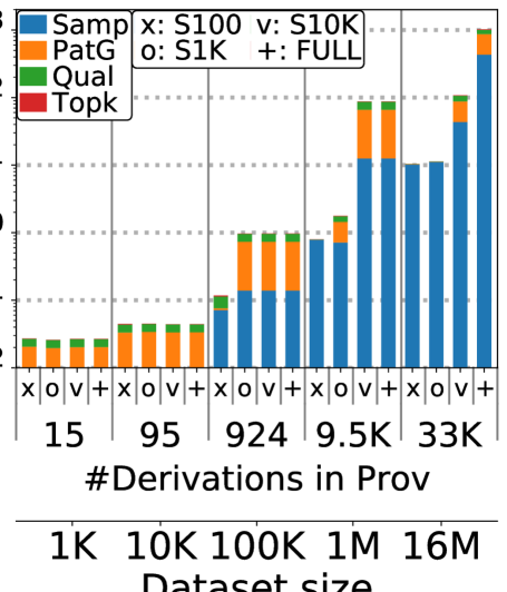
(a) $\mathtt{InvalidD}$-Why

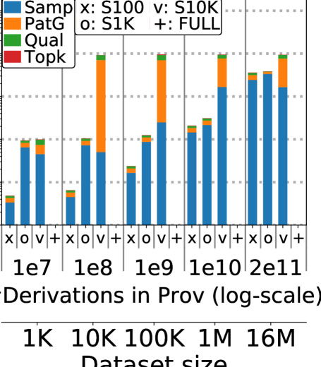
(b) $\mathtt{InvalidD}$-Whynot

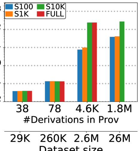
(c) $\mathtt{CasualWatch}$-Why

(d) $\mathtt{CasualWatch}$-Whynot

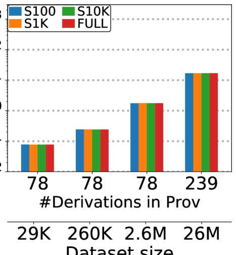
(e) $\mathtt{Players}$-Why

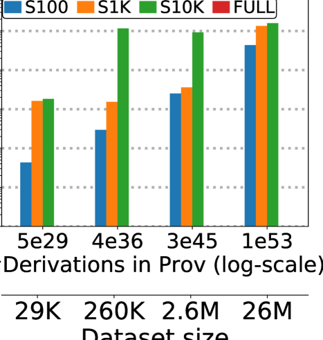
(f) $\mathtt{Players}$-Whynot

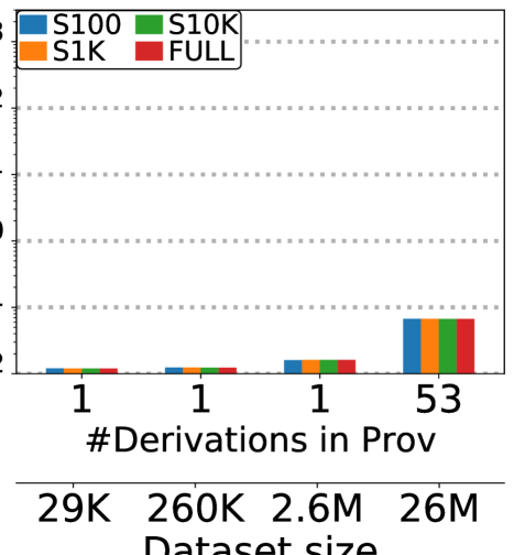
(g) $\mathtt{DirGen}$-Why

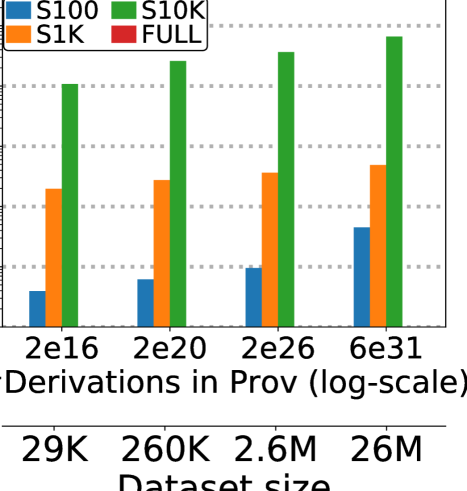
(h) $\mathtt{DirGen}$-Whynot

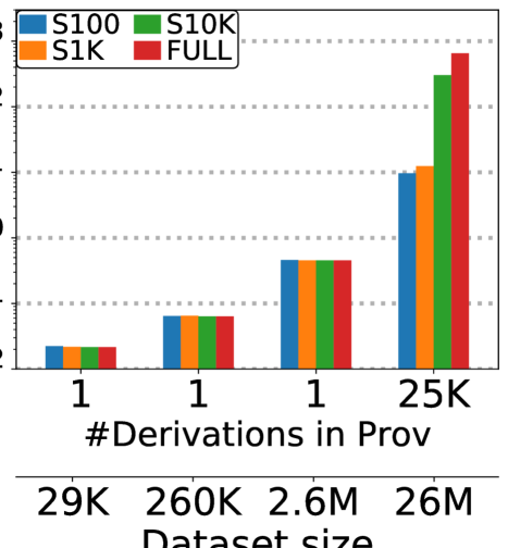
(i) $\mathtt{TomKey}$-Why

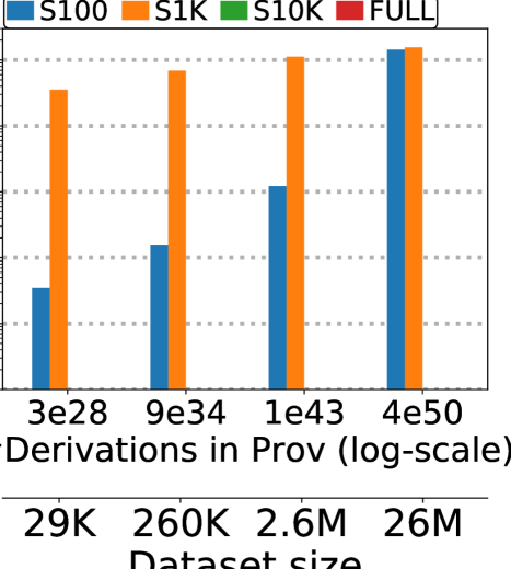
(j) $\mathtt{TomKey}$-Whynot

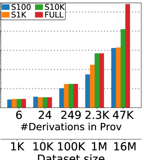
(k) $\mathtt{FavCom}$-Why

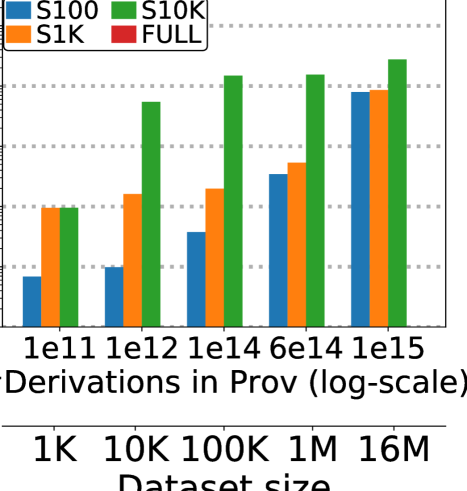
(l) $\mathtt{FavCom}$-Whynot

Figure 8: Measuring performance of generating summaries for why and why-not provenance for queries

9.1 Performance

We consider samples of varying size (Sx denotes a sample with $x$ rows). Furthermore, Full denotes using the full provenance as input for summarization. Missing bars indicate timed-out experiments ($30$ minute default timeout).

Dataset Size. We measure the runtime of our approach for computing top-$3$ summaries varying dataset and sample size over the queries from Fig. 5. On the x-axis of plots, we show both the provenance size (#derivations) and dataset size (#rows). In Fig. 8a and 8b, we show the runtimes of the individual steps of our algorithm (sampling, pattern generation, computation of quality metrics, and computing the top-3 summary) for query $r_{1}$ when using a provenance question that binds $C$ to new york (why) and swanton (why-not), respectively (the bindings for provenance questions are shown in Fig. 6). Observe that, even for the largest dataset, we are able to generate summaries within reasonable time if using sampling. Overall, pattern generation dominates the runtime for why provenance. For why-not provenance, sampling dominates the runtime for smaller sample sizes while pattern generation is dominant for S10K. FULL does not finish even for the smallest license dataset (1K). For queries $r_{3}$ (many joins with a negation) and $r_{4}$ (union of $r_{4}^{\prime}$ and $r_{4}^{\prime\prime}$), Fig. 8c and 8e show the runtimes for why and Fig. 8d and 8f show the runtimes for why-not. We observe the same trend as for $r_{1}$ even though why-not provenance is significantly larger (up to $10^{52}$ derivations). This trend is preserve over the runtimes of other queries $r_{5}$, $r_{6}$, and $r_{7}$ (Fig. 8k, 8g and 8i for why and Fig. 8l, 8h and 8j for why-not, respectively).

Performance Comparison with Naive Approach. We also compare the performance of our sample-based summaries to the summary over full provenance (FULL). The FULL is shown as ‘+’ or red bars in Fig. 8. The results of FULL for why provenance are quadratic increase over the size of successful derivations while summaries result in almost linear increase. Computing summaries over FULL why-not provenance are not feasible within the allocated time slot for any size ( bars are omitted in Fig. 8).

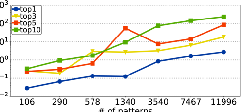
Figure 9: Runtime for computing top-$k$ summaries when patterns are provided as input.

Generating Top-$k$ summaries. Fig. 9 shows the runtime of computing the top-$k$ summary over the patterns produced by the first three steps (Sec. 5 through Sec. 7). We selected sets of patterns from different queries and sample sizes to get a roughly exponential progression of the number of patterns. We vary $k$ from $1$ to $10$. The runtime is roughly linear in $k$ and in the number of patterns. Note that this is significantly better than the theoretical worst-case of our algorithm ($O({n^{k}})$ where $n$ is the number of patterns). The reason is that typically a large number of patterns is clearly inferior and will be pruned by our algorithm early on.

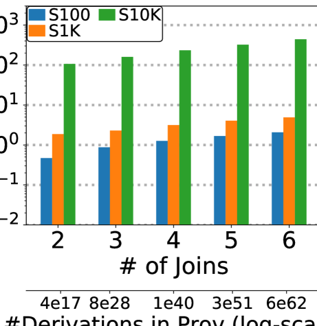
(a) Chain query

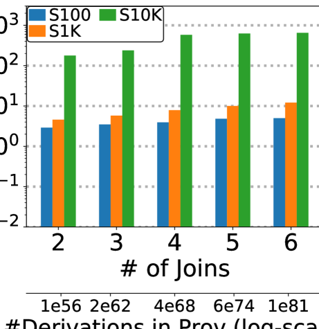
(b) Star query

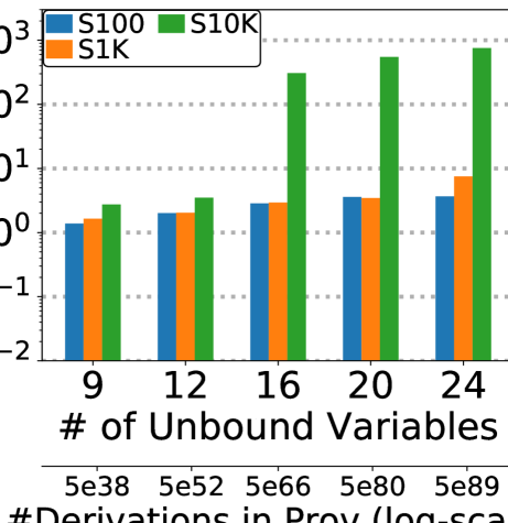
(c) Chain query

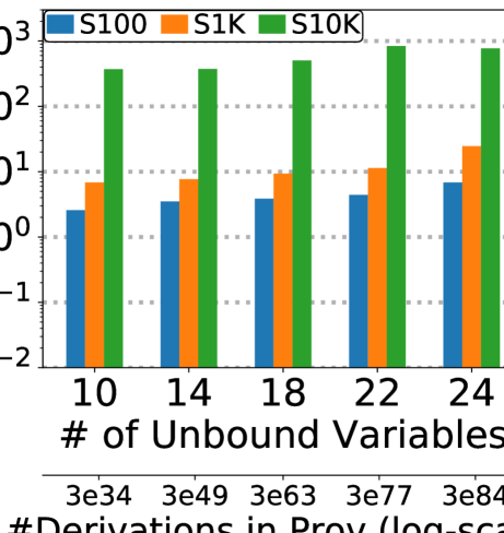
(d) Star query

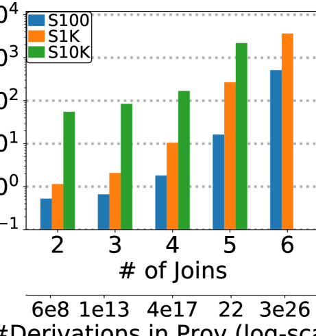
(e) $r_{11}$ over $\text{DBLP}_{100\text{K}}$

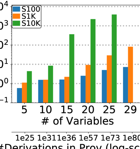
(f) $r_{12}$ over $\text{TPC-H}_{150\text{K}}$

Figure 10: Varying #joins and #variables for why-not

Query Complexity and Structure. In this experiment, we vary the query complexity in terms of number of joins and variables. We randomly generated synthetic queries whose join graph is either a star or a chain. We compute the top-3 patterns for why-not provenance. In Fig. 10a and 10b we vary the number of joins. The results confirm that our approach scales to very large provenance sizes (more than $10^{60}$ derivations) regardless of join types. To evaluate the impact of the number of variables on performance, we use chain queries with $8$-way joins and star queries with $5$-way joins. We vary the number of variables bound to constants by the query from $1$ to $16$ (out of $25$ variables). The head and join variables are never bound. The results shown in Fig. 10c and 10d confirm that our approach works well, even for queries with up to $24$ unbound variables (provenance sizes of up to $\sim 10^{80}$).

We now extend the evaluation with other queries and datasets. For the extension of variable impacts, we use query $r_{12}$ (the join size is fixed to $3$) over $\text{TPC-H}_{\text{150K}}$ and compute summaries of why-not provenance. By binding an increasing number of variables from $r_{12}$ to constants, we generate 6 rules that contain between $5$ and $29$ existential variables. The result shown in Fig. 10f confirms that our approach scales well over TPC-H dataset. Using the $\text{DBLP}_{\text{100K}}$ dataset, we vary the number of joins (path length) of query $r_{11}$. For example, $\mathtt{2Hop}(L)\,\mathtt{{:}-}\,\mathtt{DBLP}(L,R),$ $\mathtt{DBLP}(R,R1)$ is the query we use for a $2$-way join. We use a p-tuple that binds $L=\textsf{xueni pan}$ (Fig. 6). Fig. 10e shows that even for real-world dataset (with a 6-way join where the provenance contains $3\cdot 10^{26}$ derivations), we produce a summary for sample sizes S100 and S1K.

(a) Why ($\mathtt{InvalidD}$)

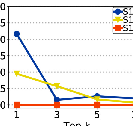
(b) Why-not ($\mathtt{InvalidD}$)

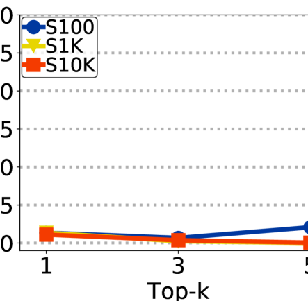
(c) Why ($\mathtt{CrimeSince}$)

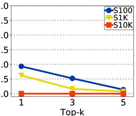
(d) Why-not ($\mathtt{CrimeSince}$)

Figure 11: Quality metric error caused by sampling.

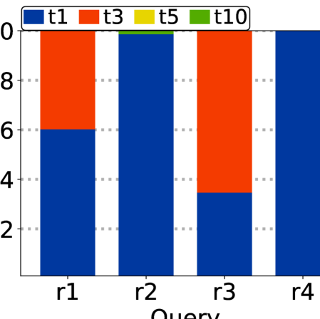
(a) Why

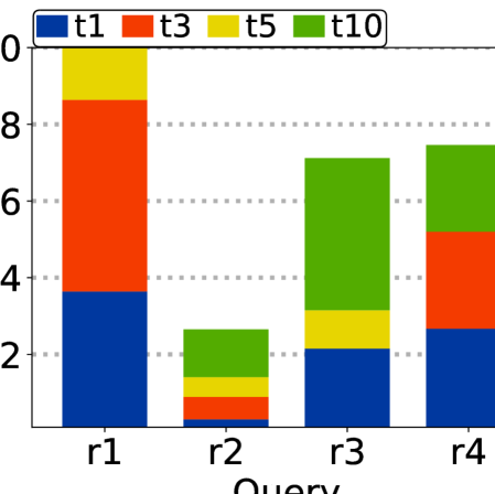
(b) Why-not

Figure 12: Completeness - varying $k$.

9.2 Pattern Quality

We now measure the difference between the quality metrics approximated using sampling and the exact values when using full provenance. For why-not provenance where it is not feasible to compute full provenance, we compare against the largest sample size (S10k) instead.

Quality Metric Error. Fig. 11a and 11b show the relative quality metric error for query $r_{1}$ over $\mathtt{InvalidD}_{\text{100K}}$ varying sample size and $k$. The error is at most $\sim$ 2% and typically decreases in $k$. For query $r_{10}$ over $\mathtt{Crimes}_{\text{1M}}$, Fig. 11c and 11d show the results for why and why-not, respectively. Similarly, the overall relative error caused by sampling is quite low (below 1%) and descreases in $k$ and sample size.

Summary Completeness. Fig. 12 shows the completeness scores of summaries returned by our approach for queries from Fig. 5. We measure this by calculating the upper bound of completeness of the set of top-$k$ patterns for each query as described in Sec. 8. For $k=10$, we achieve $100\%$ completeness for why provenance and $\sim 75\%$ completeness for why-not except for $r_{2}$ (Fig. 12b) for which the relatively large number of distinct values for the domains of unbound variables prevents us from achieving better completeness scores.

9.3 Comparisons with other systems

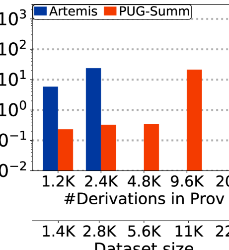
(a) Artemis

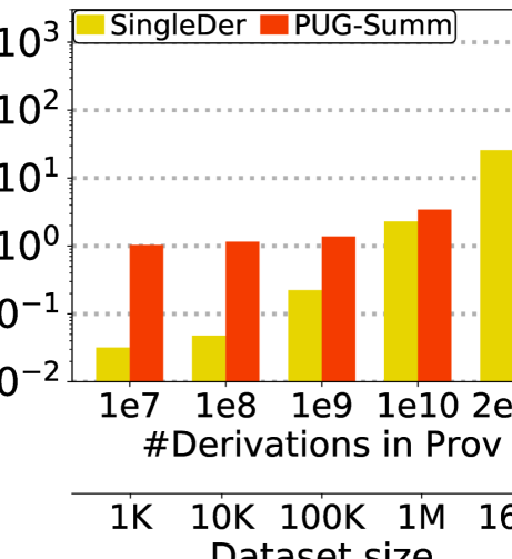
(b) Single-derivation

Figure 13: Performance comparisons for why-not

We now compare our system against [12] (all-derivations) and a single-derivation approach implemented in our system.

Artemis. The authors of [12] made their system Artemis available as a virtual machine (VM). We ran both systems in this VM (4GB memory) and used Postgres as a backend since it is supported by both systems. We used a query from the VM installation that computes the names of witnesses ($N$) who saw a person with a particular cloth and hair color ($C$ and $H$) perpetrating a crime of a particular type $T$.

$$\mathtt{CrimeDesc}( T,N,C,H)\,\mathtt{{:}-}\,\mathtt{CRIME}(T,S),\mathtt{WITNESS}(N,S),$$

$$\mathtt{SAWPERSON}(N,H,C),\mathtt{PERSON}(M,H,C),S>97$$

We use the provenance question provided by Artemis which bounds all head variables: $T$ = ‘trespassing’, $N$ = ‘aarongolden’, $C$ = ‘midnightblue’, and $H$ = ‘lavender’. The original dataset is $\mathtt{CRIME_{\text{1.4K}}}$ which we scaled up to $\mathtt{CRIME_{\text{22K}}}$. We use $\sim 10\%$ as the sample size (e.g., S2K for $\mathtt{CRIME_{\text{22K}}}$) and compute top-5 summaries. The result of this comparison is shown in Fig. 13a. Our system (PUG-Summ) outperforms Artemis by $\sim 2$ orders of magnitude for the two smallest datasets for which Artemis did not time out. Artemis returned the most general pattern (all placeholders) as the top-1 explanation:

$$p =(\textsf{tresp.},\textsf{aarongolden},\textsf{midnightblue},\textsf{lavender},S,M),S>97$$

Unlike Artemis, PUG returned a summary that contains a pattern which covers $\sim 50\%$ of the provenance:

$$p^{\prime}=(\textsf{tresp.},\textsf{aarongolden},\textsf{midnightblue},\textsf{lavender},\textsf{98},M)$$

Single Derivation Approach. We implemented a simple single-derivation approach (SingleDer) in our system by applying $n_{\textsc{S}}=1$. That is, the explanation is computed based on only one value from $\mathbb{D}$ for each unbound variable. We use query $r_{1}$ from Fig. 5, sample size S1K, and compute a top-3 summary. As shown in Fig. 13b, SingleDer outperforms PUG-Summ about an order of magnitude for small datasets. The gap between the two approaches is less significant for larger datasets (more than 1M tuples).

10 Related Work

inline,color=green!60]Deleted for revision:Our work is closely related to approaches for compactly representing provenance and explaining missing answers.

Compact Representation of Provenance. The need for compressing provenance to reduce its size has been recognized early-on, e.g., [3, 7, 22]. However, the compressed representations produced by these approaches are often not semantically meaningful to users. More closely related to our work are techniques for generating higher-level explanations for binary outcomes [8, 29], missing answers [26], or query results [24, 30, 2] as well as methods for summarizing data or general annotations which may or may not encode provenance information [33]. Specifically, like  [8, 29, 24, 30] we use patterns with placeholders. Some approaches use ontologies [26, 29] or logical constraints [24, 8, 30] to derive semantically meaningful and compact representations of a set of tuples. The use of constraints to compactly represent large or even infinite database instances has a long tradition [14, 17] and these techniques have been adopted to compactly explain missing answers [12, 23]. However, the compactness of these representations comes at the cost of computational intractability.

Missing Answers. The missing answer problem was first stated for query-based explanations (which parts of the query are responsible for the failure to derive the missing answer) in the seminal paper by Chapman et al. [6]. Most follow-up work [4, 5, 6, 27] is based on this notion. Huang et al. [13] first introduced an instance-based approach, i.e., which existing and missing input tuples caused the missing answer [12, 13, 18, 20]). Since then, several techniques have been developed to exclude spurious explanations and to support larger classes of queries [12]. As mentioned before, approaches for instance-based explanations use either the all-derivations (giving up performance) or the single-derivation approach (giving up completeness). In contrast, using summarizes we guarantee performance by compactly representing large amounts of provenance without forsaking completeness. Artemis [12] uses c-tables to compactly represent sets of missing answers. However, this comes at the cost of additional computational complexity.

11 Conclusions

We have presented an approach for efficiently computing summaries of why and why-not provenance. Our approach uses sampling to generate summaries that are guaranteed to be concise while balancing completeness (the fraction of provenance covered) and informativeness (new information provided by the summary). Thus, we overcome a severe limitation of prior work which sacrifices either completeness or performance. inline,color=green!60]Deleted for revision:A core idea of our method is to integrate sampling into provenance capture and summarization. We demonstrate experimentally that our approach efficiently produces meaningful summaries of provenance graphs with up to $10^{80}$ derivations. inline,color=green!60]Deleted for revision:Our experimental evaluation confirms that this is quite effective. We produce meaningful summaries over very large provenance (up to $10^{80}$ derivations) in only a few minutes. In future work, we plan to investigate how to utilize additional information, e.g., integrity constraints, in the summarization process.

References

- [1] M. Abramowitz and I. A. Stegun. Handbook of mathematical functions: with formulas, graphs, and mathematical tables, volume 55. Courier Corporation, 1965.
- [2] E. Ainy, P. Bourhis, S. Davidson, D. Deutch, and T. Milo. Approximated summarization of data provenance. In CIKM, pages 483–492, 2015.
- [3] M. K. Anand, S. Bowers, T. McPhillips, and B. Ludäscher. Efficient Provenance Storage over Nested Data Collections. In EDBT, pages 958–969, 2009.
- [4] N. Bidoit, M. Herschel, and K. Tzompanaki. Immutably answering why-not questions for equivalent conjunctive queries. In TaPP, 2014.
- [5] N. Bidoit, M. Herschel, K. Tzompanaki, et al. Query-Based Why-Not Provenance with NedExplain. In EDBT, pages 145–156, 2014.
- [6] A. Chapman and H. V. Jagadish. Why Not? In SIGMOD, pages 523–534, 2009.
- [7] A. Chapman, H. V. Jagadish, and P. Ramanan. Efficient Provenance Storage. In SIGMOD, pages 993–1006, 2008.
- [8] K. El Gebaly, P. Agrawal, L. Golab, F. Korn, and D. Srivastava. Interpretable and informative explanations of outcomes. PVLDB, 8(1):61–72, 2014.
- [9] K. E. Gebaly, G. Feng, L. Golab, F. Korn, and D. Srivastava. Explanation tables. IEEE Data Eng. Bull., 41(3):43–51, 2018.
- [10] T. Green, G. Karvounarakis, and V. Tannen. Provenance semirings. In PODS, pages 31–40, 2007.
- [11] M. Herschel, R. Diestelkämper, and H. Ben Lahmar. A survey on provenance: What for? what form? what from? VLDB J., 26(6):881–906, 2017.
- [12] M. Herschel and M. Hernandez. Explaining Missing Answers to SPJUA Queries. PVLDB, 3(1):185–196, 2010.
- [13] J. Huang, T. Chen, A. Doan, and J. F. Naughton. On the provenance of non-answers to queries over extracted data. PVLDB, 1(1):736–747, 2008.
- [14] T. Imieliński and W. Lipski Jr. Incomplete Information in Relational Databases. JACM, 31(4):761–791, 1984.
- [15] Y. Ioannidis. The history of histograms (abridged). In VLDB, pages 19–30, 2003.
- [16] S. Köhler, B. Ludäscher, and D. Zinn. First-order provenance games. In In Search of Elegance in the Theory and Practice of Computation, pages 382–399. Springer, 2013.
- [17] G. M. Kuper, L. Libkin, and J. Paredaens, editors. Constraint Databases. Springer, 2000.
- [18] S. Lee, S. Köhler, B. Ludäscher, and B. Glavic. A SQL-middleware unifying why and why-not provenance for first-order queries. In ICDE, pages 485–496, 2017.
- [19] S. Lee, B. Ludäscher, and B. Glavic. Provenance summaries for answers and non-answers. PVLDB, 11(12):1954–1957, 2018.
- [20] S. Lee, B. Ludäscher, and B. Glavic. Pug: a framework and practical implementation for why and why-not provenance. VLDB J., pages 1–25, 2018.
- [21] S. Lee, X. Niu, B. Ludäscher, and B. Glavic. Integrating approximate summarization with provenance capture. In TaPP, pages 2–2, 2017.
- [22] D. Olteanu and J. Závodný. On factorisation of provenance polynomials. In TaPP, 2011.
- [23] S. Riddle, S. Köhler, and B. Ludäscher. Towards constraint provenance games. In TaPP, 2014.
- [24] S. Roy and D. Suciu. A formal approach to finding explanations for database queries. In SIGMOD, pages 1579–1590, 2014.
- [25] V. Tannen. Provenance analysis for FOL model checking. ACM SIGLOG News, 4(1):24–36, 2017.
- [26] B. ten Cate, C. Civili, E. Sherkhonov, and W.-C. Tan. High-level why-not explanations using ontologies. In PODS, pages 31–43, 2015.
- [27] Q. T. Tran and C.-Y. Chan. How to conquer why-not questions. In SIGMOD, pages 15–26, 2010.
- [28] E. Von Collani and K. Dräger. Binomial distribution handbook for scientists and engineers. Springer Science & Business Media, 2001.
- [29] X. Wang, X. L. Dong, and A. Meliou. Data x-ray: A diagnostic tool for data errors. In SIGMOD, pages 1231–1245, 2015.
- [30] E. Wu and S. Madden. Scorpion: Explaining away outliers in aggregate queries. PVLDB, 6(8):553–564, 2013.
- [31] Y. Wu, A. Haeberlen, W. Zhou, and B. T. Loo. Answering why-not queries in software-defined networks with negative provenance. In Proceedings of the Twelfth ACM Workshop on Hot Topics in Networks, page 3. ACM, 2013.
- [32] Y. Wu, M. Zhao, A. Haeberlen, W. Zhou, and B. T. Loo. Diagnosing missing events in distributed systems with negative provenance. In SIGCOMM, pages 383–394, 2014.
- [33] D. Xiao and M. Y. Eltabakh. Insightnotes: Summary-based annotation management in relational databases. In SIGMOD, pages 661–672, 2014.