Convergence rate analysis and improved iterations for numerical radius computation

Abstract

The main two algorithms for computing the numerical radius are the level-set method of Mengi and Overton and the cutting-plane method of Uhlig. Via new analyses, we explain why the cutting-plane approach is sometimes much faster or much slower than the level-set one and then propose a new hybrid algorithm that remains efficient in all cases. For matrices whose fields of values are a circular disk centered at the origin, we show that the cost of Uhlig’s method blows up with respect to the desired relative accuracy. More generally, we also analyze the local behavior of Uhlig’s cutting procedure at outermost points in the field of values, showing that it often has a fast Q-linear rate of convergence and is Q-superlinear at corners. Finally, we identify and address inefficiencies in both the level-set and cutting-plane approaches and propose refined versions of these techniques.

Key words: field of values, numerical range and radius, transient behavior

Notation: $\|\cdot\|$ denotes the spectral norm, $\Lambda(\cdot)$ the spectrum (the set of eigenvalues) of a square matrix, and $\lambda_{\mathrm{max}}(\cdot)$ and $\lambda_{\mathrm{min}}(\cdot)$, respectively, the largest and smallest eigenvalue of a Hermitian matrix. $\mathrm{e}$ and $\mathbf{i}$ respectively denote Euler’s number and $\sqrt{-1}$.

1 Introduction

Consider the discrete-time dynamical system

$$x_{k+1}=Ax_{k},$$ (1.1)

where $A\in\mathbb{C}^{n\times n}$ and $x_{k}\in\mathbb{C}^{n}$. The asymptotic behavior of (1.1) is of course characterized by the moduli of $\Lambda(A)$. Given the spectral radius of $A$,

$$\rho(A)\coloneqq\max\{|\lambda|:\lambda\in\Lambda(A)\},$$ (1.2)

$\lim_{k\to\infty}\|x_{k}\|=0$ for all $x_{0}$ if and only if $\rho(A)<1$, with the asymptotic decay rate being faster the closer $\rho(A)$ is to zero. However, knowing the transient behavior of (1.1) is often of interest. Clearly, the trajectory of (1.1) is tied to powers of $A$, since $x_{k}=A^{k}x_{0}$ and so $\|x_{k}\|\leq\|A^{k}\|\|x_{0}\|$. Indeed, a central theme of Trefethen and Embree’s treatise on pseudospectra [TE05] is how large $\sup_{k\geq 0}\|A^{k}\|$ can be.

One perspective is given by the field of values (numerical range) of $A$,

$$W(A)\coloneqq\{x^{*}Ax:x\in\mathbb{C}^{n},\|x\|=1\}.$$ (1.3)

Consider the maximum of the moduli of points in $W(A)$, i.e., the numerical radius

$$r(A)\coloneqq\max\{|z|:z\in W(A)\}.$$ (1.4)

It is known that $\tfrac{1}{2}\|A\|\leq r(A)\leq\|A\|$; see [HJ91, p. 44]. Combining the lower bound with the power inequality $r(A^{k})\leq(r(A))^{k}$ [Ber65, Pea66] yields

$$\|A^{k}\|\leq 2(r(A))^{k}.$$ (1.5)

As $2(r(A))^{k}\leq\|A\|^{k}$ if and only if $r(A)\leq\sqrt[k]{0.5}\|A\|$, and $r(A)\leq\|A\|$ always holds, it follows that $2(r(A))^{k}$ is often a tighter upper bound for $\|A^{k}\|$ than $\|A\|^{k}$ is, and so the numerical radius can be useful in estimating the transient behavior of (1.1).

The concept of the numerical radius dates to at least 1961; see [LO20, p. 1005]. In 1978, Johnson noted that $r(A)$ could be computed via his cutting-plane technique to approximate $W(A)$, but that a modified algorithm would likely be more efficient [Joh78, Remark 3]. Such geometric approaches estimate $W(A)$ (or $r(A)$) by computing a number of supporting hyperplanes to sufficiently approximate the boundary of $W(A)$ (or regions of it); supporting hyperplanes are computed using the much earlier Bendixson-Hirsch theorem [Ben02] and fundamental results of Kippenhahn [Kip51]. Results related to computing $r(A)$ also appeared in the 1990s. Mathias showed that $r(A)$ can be obtained by solving a semidefinite program [Mat93], but doing so is expensive. Much faster algorithms were then proposed by He and Watson [Wat96, HW97], but these methods may not converge to $r(A)$.

The 2000s saw further interest in computing $r(A)$ with the following key results. In 2005, Mengi and Overton gave a fast globally convergent method for $r(A)$ [MO05] by combining an idea of He and Watson [HW97] with the level-set approach of Boyd, Balakrishnan, Bruinsma, and Steinbuch (BBBS) [BB90, BS90] for computing the $\mathcal{H}_{\infty}$ norm. Although Mengi and Overton observed that their method converged quadratically, this was only later proved in 2012 by Gürbüzbalaban in his PhD thesis [Gür12, section 3.4]. Meanwhile, in 2009, Uhlig proposed a fast geometric approach to computing $r(A)$ [Uhl09] using cutting planes and a new greedy strategy. A major benefit of cutting-plane methods is that they only require computing $\lambda_{\mathrm{max}}$ of $n\times n$ Hermitian matrices. If $A$ is sparse, this can be done efficiently and reliably using, say, eigs in MATLAB. Hence, Uhlig’s method can be used on large-scale problems while still being globally convergent. In contrast, at every iteration, the level-set approach requires solving a generalized eigenvalue problem of order $2n$, which by standard convention on work complexity, is an atomic operation with $\mathcal{O}(n^{3})$ work. While Uhlig noted that convergence of his method can sometimes be quite slow [Uhl09, p. 344], his experiments in the same paper showed several problems where his cutting-plane method was decisively faster Mengi and Overton’s level-set method.

A key motivation for our work here is the class of problems where the numerical radius of parametric matrices is optimized, such as feedback control; see [LO20] for more details and other applications. Since minimizing the numerical radius is a nonsmooth optimization problem, optimization solvers generally will converge slowly and require many function evaluations. During the course of optimization, the numerical radius will be computed for many different parameter choices, and the shape and location of the field of values will be constantly changing. Per [LO20], the solutions to such numerical radius optimization problems are often so-called disk matrices; a disk matrix is one whose field of values is a disk centered at the origin. As we elucidate in this paper, whether a cutting-plane method is very fast or very slow is determined by the geometry of the field of values, and for disk matrices, the overall cost of a cutting-plane method blows up with respect to the desired relative accuracy. For optimizing the numerical radius, we thus would like to have a numerical radius method that remains efficient in all cases, which is what we propose here. Moreover, we want such consistent efficiency without sacrificing the precision afforded by the hardware. As we show later, one can avoid the high costs of cutting-plane methods if one settles for only a few digits of accuracy, but doing so can adversely affect the quality and reliability of optimization. Inaccuracy in the estimates of the numerical radius values can cause optimization solvers to stagnate (e.g., line searches may break down), while computed gradients, which are critical, of $\max$ functions can be totally inaccurate even when the function values are computed to, say, seven digits; for more details, see [BM18] and [BMO18].

The paper is organized as follows. In Section 2, we give necessary preliminaries on the field of values, the numerical radius, and earlier $r(A)$ algorithms. We then identify and address some inefficiencies in the level-set method of Mengi and Overton and propose a faster variant in Section 3. We analyze Uhlig’s method in Section 4, deriving (a) its overall cost when the field of values is a disk centered at the origin, and (b) a Q-linear local rate of convergence result for its cutting procedure. These analyses precisely show how, depending on the problem, Uhlig’s method can be either extremely fast or extremely slow. In Section 5, we identify an inefficiency in Uhlig’s cutting procedure and address it via a more efficient cutting scheme whose exact convergence rate we also derive. Putting all of this together, we present our new hybrid algorithm in Section 6. We validate our results experimentally in Section 7 and give concluding remarks in Section 8.

2 Preliminaries

We will need the following well-known facts [Kip51, HJ91]:

Remark 2.1.

Given $A\in\mathbb{C}^{n\times n}$,

1. $W(A)\subset\mathbb{C}$ is a compact, convex set,

2. if $A$ is real, then $W(A)$ has real axis symmetry,

3. if $A$ is normal, then $W(A)$ is the convex hull of $\Lambda(A)$,

4. $W(A)=[\lambda_{\mathrm{min}}(A),\lambda_{\mathrm{max}}(A)]$ if and only if $A$ is Hermitian,

5. the boundary of $W(A)$, $\partial W(A)$, is a piecewise smooth algebraic curve,

6. if $v\in\partial W(A)$ is a point where $\partial W(A)$ is not differentiable, i.e., a corner, then $v\in\Lambda(A)$. Corners always correspond to two line segments in $\partial W(A)$ meeting at some angle less than $\pi$ radians.

Definition 2.2.

Given a nonempty closed set $\mathcal{D}\subset\mathbb{C}$, a point $\tilde{z}\in\mathcal{D}$ is (globally) outermost if $|\tilde{z}|=\max\{|z|:z\in\mathcal{D}\}$ and locally outermost if $\tilde{z}$ is an outermost point of $\mathcal{D}\cap\mathcal{N}$, for some neighborhood $\mathcal{N}$ of $\tilde{z}$.

For continuous-time systems $\dot{x}=Ax$, we have the numerical abscissa

$$\alpha_{W}(A)\coloneqq\max\{\mathrm{Re}\,z:z\in W(A)\},$$ (2.1)

i.e., the maximal real part of all points in $W(A)$. Unlike the numerical radius, computing the numerical abscissa is straightforward, as [HJ91, p. 34]

$$\alpha_{W}(A)=\lambda_{\mathrm{max}}\left(\tfrac{1}{2}\left(A+A^{*}\right)\right).$$ (2.2)

For $\theta\geq 0$, $W(\mathrm{e}^{\mathbf{i}\theta}A)$ is $W(A)$ rotated counter-clockwise about the origin. Consider

$$H(\theta)\coloneqq\tfrac{1}{2}\left(\mathrm{e}^{\mathbf{i}\theta}A+\mathrm{e}^{-\mathbf{i}\theta}A^{*}\right),$$ (2.3)

so $\alpha_{W}(\mathrm{e}^{\mathbf{i}\theta}A)=\lambda_{\mathrm{max}}(H(\theta))$ and $\alpha_{W}(A)=\lambda_{\mathrm{max}}(H(0))$. Let $\lambda_{\theta}$ and $x_{\theta}$ denote, respectively, $\lambda_{\mathrm{max}}(H(\theta))$ and an associated normalized eigenvector. Furthermore, let $L_{\theta}$ denote the line $\{\mathrm{e}^{-\mathbf{i}\theta}(\lambda_{\theta}+\mathbf{i}t):t\in\mathbb{R}\}$ and $P_{\theta}$ the half plane $\mathrm{e}^{-\mathbf{i}\theta}\{z:\mathrm{Re}\,z\leq\lambda_{\theta}\}$. Then $L_{\theta}$ is a supporting hyperplane for $W(A)$ and [Joh78, p. 597]

1. $W(A)\subseteq P_{\theta}$ for all $\theta\in[0,2\pi)$,

2. $W(A)=\cap_{\theta\in[0,2\pi)}P_{\theta}$,

3. $z_{\theta}=x_{\theta}^{*}Ax_{\theta}\in L_{\theta}$ is a boundary point of $W(A)$.

As $H(\theta+\pi)=-H(\theta)$, $P_{\theta+\pi}$ can also be obtained via $\lambda_{\mathrm{min}}(H(\theta))$ and an associated eigenvector. The Bendixson-Hirsch theorem is a special case of these properties, defining the bounding box of $W(A)$ for $\theta=0$ and $\theta=\tfrac{\pi}{2}$.

When $\lambda_{\mathrm{max}}(H(\theta))$ is simple, the following result of Fiedler [Fie81, Theorem 3.3] gives a formula for computing the radius of curvature $\tilde{r}$ of $\partial W(A)$ at $z_{\theta}$, defined as the radius of the osculating circle of $\partial W(A)$ at $z_{\theta}$, i.e., the circle with the same tangent and curvature as $\partial W(A)$ at $z_{\theta}$. At corners of $\partial W(A)$, we say that $\tilde{r}=0$, while at other boundary points where the radius of curvature is well defined, $\tilde{r}>0$ and becomes infinite at points inside line segments in $\partial W(A)$. Although the formula is given for $\theta=0$ and $z_{\theta}=0$, by simple rotation and shifting, it can be applied generally. See Fig. 1a for a depiction of the osculating circle of $\partial W(A)$ at an outermost point in $W(A)$.

Theorem 2.3 (Fiedler).

Let $H_{1}=\tfrac{1}{2}(A+A^{*})$, $H_{2}=\tfrac{1}{2\mathbf{i}}(A-A^{*})$, let $H_{1}^{+}$ be the Moore-Penrose pseudoinverse of $H_{1}$, and let $x_{\theta}$ be a normalized eigenvector corresponding to $\lambda_{\mathrm{max}}(H(\theta))$. Noting that $A=H_{1}+\mathbf{i}H_{2}$ and $H(0)=H_{1}$, suppose that $\lambda_{\mathrm{max}}(H_{1})=0$ and is simple, and that the associated boundary point $z_{\theta}=x_{\theta}^{*}Ax_{\theta}=0$, where $\theta=0$. Then the radius of curvature of $\partial W(A)$ at $z_{\theta}$ is

$$\tilde{r}=-2(H_{2}x_{\theta})^{*}H_{1}^{+}(H_{2}x_{\theta}).$$ (2.4)

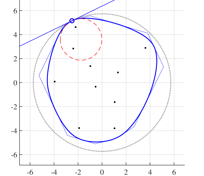
(a) The field of values and local curvature.

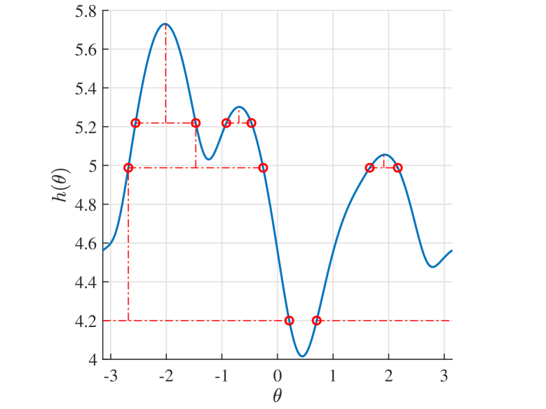
(b) Level-set iterates for $h(\theta)$.

Figure 1: For a random matrix $A\in\mathbb{C}^{10\times 10}$, the left and right panes respectively show $\partial W(A)$ (blue curve) and $h(\theta)$ (blue plot). On the left, the following are also shown: $\Lambda(A)$ (black dots), a polygonal approximation $\mathcal{G}_{j}$ to $W(A)$ (blue polygon), the outermost point in $W(A)$ (small blue circle) with the corresponding supporting hyperplane (blue line) and osculating circle (dashed red circle), and the circle of radius $r(A)$ centered at the origin (black dotted circle). On the right, three iterations of the level-set method are also shown (small circles and dash-dotted lines in red).

Via (2.2) and (2.3), the numerical radius can be written as

$$r(A)=\max_{\theta\in[0,2\pi)}h(\theta)\qquad\text{where}\qquad h(\theta)\coloneqq\lambda_{\mathrm{max}}\left(H(\theta)\right),$$ (2.5)

i.e., a one-variable maximization problem. Via $H(\theta+\pi)=-H(\theta)$, it also follows that

$$r(A)=\max_{\theta\in[0,\pi)}\rho(H(\theta)).$$ (2.6)

However, as (2.5) and (2.6) may have multiple maxima, it is not straightforward to find a global maximizer of either, and crucially, assert that it is indeed a global maximizer in order to verify that $r(A)$ has been computed. Per (A3), we generally assume that $A$ is non-normal, as otherwise $r(A)=\rho(A)$.

We now discuss earlier numerical radius algorithms in more detail. In 1996, Watson proposed two $r(A)$ methods [Wat96]: one which converges to local maximizers of (2.6) and a second which lacks convergence guarantees but is cheaper (though they each do $\mathcal{O}(n^{2})$ work per iteration). However, as both iterations are related to the power method, they may exhibit very slow convergence, and the cheaper iteration may not converge at all. Shortly thereafter [HW97], He and Watson used the second iteration (because it was cheaper) in combination with a new certificate test inspired by Byers’ distance to instability algorithm [Bye88]. This certificate either asserts that $r(A)$ has been computed to a desired accuracy or provides a way to restart Watson’s cheaper iteration with the hope of more accurately estimating $r(A)$. However, He and Watson’s method is still not guaranteed to converge, since Watson’s cheaper iteration may not converge. Inspired by the BBBS algorithm for computing the $\mathcal{H}_{\infty}$ norm, Mengi and Overton then proposed a globally convergent iteration for $r(A)$ in 2005 by using He and Watson’s certificate test in a much more powerful way. Given $\gamma\leq r(A)$, the test actually allows one to obtain the $\gamma$-level set of $h(\theta)$, i.e., $\{\theta:h(\theta)=\gamma\}$. Assuming the level set is not empty, Mengi and Overton’s method then evaluates $h(\theta)$ at the midpoints of the intervals under $h(\theta)$ determined by the $\gamma$-level set points. Estimate $\gamma$ is then updated (increased) to the highest of these corresponding function values. This process is done in a loop, and as mentioned in the introduction, has local quadratic convergence. See Fig. 1b for a depiction of this level-set iteration.

The certificate (or level-set) test is based on [MO05, Theorem 3.1], which is a slight restatement of [HW97, Theorem 2] from He and Watson. We omit the proof.

Theorem 2.4.

Given $\gamma\in\mathbb{R}$, the pencil $R_{\gamma}-\lambda S$ has $\mathrm{e}^{\mathbf{i}\theta}$ as an eigenvalue or is singular if and only if $\gamma$ is an eigenvalue of $H(\theta)$ defined in (2.3), where

$$R_{\gamma}\coloneqq\begin{bmatrix}2\gamma I&-A^{*}\\ I&0\end{bmatrix}\quad\text{and}\quad S\coloneqq\begin{bmatrix}A&0\\ 0&I\end{bmatrix}.$$ (2.7)

Per Theorem 2.4, the $\gamma$-level set of $h(\theta)=\lambda_{\mathrm{max}}(H(\theta))$ is associated with the unimodular eigenvalues of $R_{\gamma}-\lambda S$, which can be obtained in $\mathcal{O}(n^{3})$ work (with a significant constant factor). Note that the converse may not hold, i.e., for a unimodular eigenvalue of $R_{\gamma}-\lambda S$, $\gamma$ may correspond to an eigenvalue of $H(\theta)$ other than $\lambda_{\mathrm{max}}(H(\theta))$. Given any $\theta\in[0,2\pi)$, also note that $R_{\gamma}-\lambda S$ is nonsingular for all $\gamma>h(\theta)$. This is because if $W(A)$ and a disk centered at the origin enclosing $W(A)$ have more than $n$ shared boundary points, then $W(A)$ is that disk; see [TY99, Lemma 6].

Uhlig’s method computes $r(A)$ via updating a bounded convex polygonal approximation to $W(A)$ and set of known points in $\partial W(A)$ respectively given by:

$$\mathcal{G}_{j}\coloneqq\bigcap_{\theta\in\left\{\theta_{1},\ldots,\theta_{j}\right\}}P_{\theta}\qquad\text{and}\qquad\mathcal{Z}_{j}\coloneqq\{z_{\theta_{1}},\ldots,z_{\theta_{j}}\},$$

where $W(A)\subseteq\mathcal{G}_{j}$ (see Fig. 1a for a depiction), $0\leq\theta_{1}<\cdots<\theta_{j}<2\pi$, and $z_{\theta_{\ell}}=x_{\theta_{\ell}}^{*}Ax_{\theta_{\ell}}$ is a boundary point of $W(A)$ on $L_{\theta_{\ell}}$ for $\ell=1,\ldots,j$. Note that the corners of $\mathcal{G}_{j}$ are given by $L_{\theta_{\ell}}\cap L_{\theta_{\ell+1}}$ for $\ell=1,\ldots,j-1$ and $L_{\theta_{1}}\cap L_{\theta_{j}}$. Given $\mathcal{G}_{j}$ and $\mathcal{Z}_{j}$, lower and upper bounds $l_{j}\leq r(A)\leq u_{j}$ are immediate, where

$$l_{j}\coloneqq\max\{|b|:b\in\mathcal{Z}_{j}\}\quad\text{and}\quad u_{j}\coloneqq\max\{|c|:c\text{ a corner of }\mathcal{G}_{j}\},$$

so we define the relative error estimate:

$$\varepsilon_{j}\coloneqq\frac{u_{j}-l_{j}}{l_{j}}.$$ (2.8)

By repeatedly cutting outermost corners of $\mathcal{G}_{j}$, and in turn, adding computed boundary points of $W(A)$ to $\mathcal{Z}_{j}$, it follows that $\varepsilon_{j}$ must fall below a desired relative tolerance for some $k\geq j$; hence, $r(A)$ can be computed to any desired accuracy. Uhlig’s method achieves this via a greedy strategy. On each iteration, his algorithm chops off an outermost corner $c_{j}$ from $\mathcal{G}_{j}$, which is done via computing the supporting hyperplane $L_{\theta_{j+1}}$ for $\theta_{j+1}=-\operatorname{Arg}(c_{j})$ and the boundary point $z_{\theta_{j+1}}=x_{\theta_{j+1}}^{*}Ax_{\theta_{j+1}}$. Assuming that $c_{j}\not\in W(A)$, the cutting operation results in $\mathcal{G}_{j+1}\coloneqq\mathcal{G}_{j}\cap P_{\theta_{j+1}}$, a smaller polygonal region excluding the corner $c_{j}$, and $\mathcal{Z}_{j+1}\coloneqq\mathcal{Z}_{j}\cup\{z_{\theta_{j+1}}\}$; therefore, $\varepsilon_{j+1}\leq\varepsilon_{j}$. However, if $c_{j}$ happens to be a corner of $\partial W(A)$, then it cannot be cut from $\mathcal{G}_{j}$, and instead this operation asserts that $|c_{j}|=r(A)$, and so $r(A)$ has been computed. In Section 4, Figure 2 depicts Uhlig’s method when a corner is cut.

Remark 2.5.

Recall that the parallel supporting hyperplane $L_{\theta_{j+1}+\pi}$ and the corresponding boundary point $z_{\theta_{j+1}+\pi}$ can be obtained via an eigenvector $\tilde{x}_{\theta_{j+1}}$ of $\lambda_{\mathrm{min}}(H(\theta_{j+1}))$. If $\tilde{x}_{\theta_{j+1}}$ is already available or relatively cheap to compute, there is little reason not to also update $\mathcal{G}_{j}$ and $\mathcal{Z}_{j}$ using this additional information.

3 Improvements to the level-set approach

We now propose two straightforward but important modifications to make the level-set approach faster and more reliable. We need the following immediate corollary of Theorem 2.4, which clarifies that Theorem 2.4 also allows all points in any $\gamma$-level set of $\rho(H(\theta))$ to be computed.

Corollary 3.1.

Given $\gamma\geq 0$, if $\rho(H(\theta))=\gamma$, then there exists $\lambda\in\mathbb{C}$ such that $|\lambda|=1$, $\det(R_{\gamma}-\lambda S)=0$, and $\theta=f(\operatorname{Arg}(\lambda))$, where $f:(-\pi,\pi]\mapsto[0,\pi)$ is

$$f(\theta)\coloneqq\begin{cases}\theta+\pi&\text{if }\theta<0\\ 0&\text{if }\theta=0\text{ or }\theta=\pi\\ \theta&\text{otherwise}.\end{cases}$$ (3.1)

Thus, first we propose doing a BBBS-like iteration using $\rho(H(\theta))$ instead of $h(\theta)$, which also has local quadratic convergence. By an extension of the argument of Boyd and Balakrishnan [BB90], near maximizers, $\rho(H(\theta))$ is unconditionally twice continuously differentiable with Lipschitz second derivative; see [MO22]. Using $\rho(H(\theta))$ is also typically faster in terms of constant factors. This is because $\rho(H(\theta))\geq h(\theta)$ always holds, $\rho(H(\theta))\geq 0$ (unlike $h(\theta)$, which can be negative), and the optimization domain is reduced from $[0,2\pi)$ to $[0,\pi)$. Thus, every update to the current estimate $\gamma$ computed via $\rho(H(\theta))$ must be at least as good as the one from using $h(\theta)$ (and possibly much better), and there may also be fewer level-set intervals per iteration, which reduces the number of eigenproblems incurred involving $H(\theta)$.

Second, we also propose using local optimization on top of the BBBS-like step at every iteration, i.e., the BBBS-like step is used to initialize optimization in order to find a maximizer of $\rho(H(\theta))$. The first benefit is speed, as optimization often results in much larger updates to estimate $\gamma$ and these updates are now locally optimal. This greatly reduces the total number of expensive eigenvalue computations done with $R_{\gamma}-\lambda S$, often down to just one; hence, the overall runtime can be substantially reduced since in comparison, optimization is cheap (as we explain momentarily). The second benefit is that using optimization also avoids some numerical difficulties when solely working with $R_{\gamma}-\lambda S$ to update $\gamma$. In their 1997 paper, He and Watson showed that the condition number of a unimodular eigenvalue of $R_{\gamma}-\lambda S$ actually blows up as $\theta$ approaches critical values of $h(\theta)$ or $\rho(H(\theta))$ [HW97, Theorem 4], as this corresponds to a pair of unimodular eigenvalues of $R_{\gamma}-\lambda S$ coalescing into a double eigenvalue. Since this must always occur as a level-set method converges, rounding errors may prevent all of the unimodular eigenvalues from being detected, causing level-set points to go undetected, thus resulting in stagnation of the algorithm before it finds $r(A)$ to the desired accuracy. He and Watson wrote that their analytical result was “hardly encouraging” [HW97, p. 336], though they did not observe this issue in their experiments. However, an example of such a deleterious effect is shown in [BM19, Figure 2], where analogous eigenvalue computations are shown to greatly reduce numerical accuracy when computing the pseudospectral abscissa [BLO03].

In contrast, optimizing $\rho(H(\theta))$ does not lead to numerical difficulties. This objective function is both Lipschitz (as $H(\theta)$ is Hermitian [Kat82, Theorem II.6.8]) and smooth at its maximizers (as discussed above). Thus, local maximizers of $\rho(H(\theta))$ can be found using, say, Newton’s method, with only a handful of iterations. Interestingly, in their concluding remarks [HW97, p. 341–2], He and Watson seem to have been somewhat pessimistic about using Newton’s method, writing that while it would have faster local convergence than Watson’s iteration, “the price to be paid is at least a considerable increase in computation, and possibly the need of the calculation of higher derivatives, and for the incorporation of a line search.” As we now explain, using, say, secant or Newton’s method, is actually an overall big win. Also, note that with either secant or Newton, steps of length one are always eventually accepted; hence, the cost of line searches should not be a concern.

Algorithm 3.1 An Improved Level-Set Algorithm

0:   $A\in\mathbb{C}^{n\times n}$ with $n\geq 2$, initial guesses $\mathcal{M}=\{\theta_{1},\ldots,\theta_{q}\}$, and $\tau_{\mathrm{tol}}>0$.

0:   $\gamma$ such that $|\gamma-r(A)|\leq\tau_{\mathrm{tol}}\cdot r(A)$.  

1:  $\mathcal{M}\leftarrow\mathcal{M}\cup\{0\}$

2:  while  $\mathcal{M}$ is not empty  do

3:     $\theta_{\mathrm{BBBS}}\leftarrow\operatorname*{arg\,max}_{\theta\in\mathcal{M}}\rho(H(\theta))$ // In case of ties, just take any one

4:     $\gamma\leftarrow$ maximization of $\rho(H(\theta))$ via local optimization initialized at $\theta_{\mathrm{BBBS}}$

5:     $\gamma\leftarrow\gamma(1+\tau_{\mathrm{tol}})$

6:     $\Theta\leftarrow\{f(\operatorname{Arg}(\lambda)):\det(R_{\gamma}-\lambda S)=0,|\lambda|=1\}$

7:     $[\theta_{1},\ldots,\theta_{q}]\leftarrow\Theta~{}\text{sorted in increasing order with any duplicates removed}$

8:     $\mathcal{M}\leftarrow\{\theta:\rho(H(\theta))>\gamma~{}\text{where}~{}\theta=0.5(\theta_{\ell}+\theta_{\ell+1}),\ell=1,\ldots,q-1\}$

9:  end while

Note: For simplicity, we forgo giving pseudocode to exploit possible normality of $A$ or symmetry of $W(A)$, and assume that eigenvalues and local maximizers are obtained exactly and that the optimization solver is monotonic, i.e., it guarantees $\rho(H(\theta_{\mathrm{BBBS}}))\leq\rho(H(\theta_{\star}))$, where $\theta_{\star}$ is the maximizer computed in line 4. Recall that $f(\cdot)$ is defined in (3.1), and note that the method reduces to a BBBS-like iteration using (2.6) if line 4 is replaced by $\gamma\leftarrow\rho(H(\theta_{\mathrm{BBBS}}))$. Running optimization from other angles in $\mathcal{M}$ (in addition to $\theta_{\mathrm{BBBS}}$) every iteration may also be advantageous, particularly if this can be done via parallel processing. Adding zero to the initial set $\mathcal{M}$ avoids having to deal with any “wrap-around” level-set intervals due to the periodicity of $\rho(H(\theta))$.

Suppose $\rho(H(\theta))$ is attained by a unique eigenvalue $\lambda_{j}$ with normalized eigenvector $x_{j}$. Then by standard perturbation theory for simple eigenvalues,

$$\rho^{\prime}(H(\theta))=\operatorname{sgn}(\lambda_{j})\cdot x_{j}^{*}H^{\prime}(\theta)x_{j}=\operatorname{sgn}(\lambda_{j})\cdot x_{j}^{*}\left(\tfrac{\mathbf{i}}{2}\left(\mathrm{e}^{\mathbf{i}\theta}A-\mathrm{e}^{-\mathbf{i}\theta}A^{*}\right)\right)x_{j}.$$ (3.2)

Thus, given $\lambda_{j}$ and $x_{j}$, the additional cost of obtaining $\rho^{\prime}(H(\theta))$ mostly amounts to the single matrix-vector product $H^{\prime}(\theta)x_{j}$. To compute $\rho^{\prime\prime}(H(\theta))$, we will need the following result for second derivatives of eigenvalues; see [Lan64].

Theorem 3.2.

For $t\in\mathbb{R}$, let $A(t)$ be a twice-differentiable $n\times n$ Hermitian matrix family with, for $t=0$, eigenvalues $\lambda_{1}\geq\ldots\geq\lambda_{n}$ and associated eigenvectors $x_{1},\ldots,x_{n}$, with $\|x_{k}\|=1$ for all $k$. Then assuming $\lambda_{j}$ is unique,

$$\lambda_{j}^{\prime\prime}(t)\bigg{|}_{t=0}=x_{j}^{*}A^{\prime\prime}(0)x_{j}+2\sum_{k\neq j}\frac{|x_{k}^{*}A^{\prime}(0)x_{j}|^{2}}{\lambda_{k}-\lambda_{j}}.$$

Although obtaining the eigendecomposition of $H(\theta)$ is cubic work, this is generally negligible compared to the cost of obtaining all the unimodular eigenvalues of $R_{\gamma}-\lambda S$ when using Theorem 2.4 computationally; recall that $H(\theta)$ is an $n\times n$ Hermitian matrix, while $R_{\gamma}-\lambda S$ is a generalized eigenvalue problem of order $2n$. Moreover, $H^{\prime}(\theta)x_{j}$ would already be computed for $\rho^{\prime}(H(\theta))$, while $H^{\prime\prime}(\theta)x_{j}=-H(\theta)x_{j}=-\lambda_{j}x_{j}$, so there is no other work of consequence to obtain $\rho^{\prime\prime}(H(\theta))$ via Theorem 3.2.

Table 1: The running time of a given operation divided by the running time of eig($H(\theta)$) for random $A\in\mathbb{C}^{n\times n}$. Eigenvectors were requested for $H(\theta)$ (for computing derivatives and boundary points) but not for $R_{\gamma}-\lambda S$. For eigs, k is the number of eigenvalues requested, while ’LM’ (largest modulus), ’LR’ (largest real), and ’BE’ (both ends) specifies which eigenvalues are desired.

		eigs($H(\theta)$,k,’LM’)		eigs($H(\theta)$,k,’LR’)		eigs($H(\theta)$,k,’BE’)			eig($R_{\gamma}$,$S$)
	$n$	$\texttt{k}=1$	$\texttt{k}=6$	$\texttt{k}=1$	$\texttt{k}=6$	$\texttt{k}=2$	$\texttt{k}=4$	$\texttt{k}=6$
Dense $A$	200	$6.2$	$1.9$	$1.0$	$1.2$	$1.9$	$1.2$	$1.2$	$33.9$
	400	$0.6$	$0.9$	$0.5$	$0.8$	$0.6$	$0.7$	$0.8$	$75.2$
	800	$0.7$	$1.3$	$0.6$	$1.1$	$1.3$	$1.1$	$1.1$	$175.0$
	1600	$0.4$	$0.6$	$0.3$	$0.6$	$0.6$	$0.7$	$0.6$	$205.1$
Sparse $A$	200	$4.6$	$3.7$	$1.9$	$3.3$	$3.3$	$3.6$	$3.6$	$42.8$
	400	$2.0$	$3.1$	$1.7$	$3.0$	$3.1$	$3.2$	$3.1$	$84.1$
	800	$0.8$	$1.2$	$0.7$	$1.2$	$1.4$	$1.1$	$1.3$	$172.7$
	1600	$0.4$	$0.7$	$0.4$	$0.7$	$0.8$	$0.9$	$0.7$	$199.0$

Pseudocode for our improved level-set algorithm is given in Algorithm 3.1. We now address some implementation concerns. What method is used to find maximizers of $\rho(H(\theta))$ depends on the relative costs of solving eigenvalue problems involving $H(\theta)$ and $R_{\gamma}-\lambda S$. Table 1 shows examples where 34–205 calls of eig($H(\theta)$) can be done before the total cost exceeds that of a single call of eig($R_{\gamma}$,$S$). This highlights just how beneficial it can be to incur a few more computations with $H(\theta)$ to find local maximizers as Algorithm 3.1 does. Comparisons for computing extremal eigenvalues of $H(\theta)$ via eig and eigs are also shown in the table. Such data inform whether or not the increased cost of needing to use eig in order to compute $\rho^{\prime\prime}(H(\theta))$ is offset by the advantages that second derivatives can bring, e.g., faster local convergence. Of course, fine-grained implementation decisions like these should ideally be made via tuning, as such timings are generally also software and hardware dependent. Nevertheless, Table 1 suggests that implementing Algorithm 3.1 using Newton’s method via eig might be a bit more efficient than using the secant method for $n\leq 800$ or so.

There is one more subtle but important detail for implementing Algorithm 3.1. Suppose that $\theta_{\mathrm{BBBS}}$ in line 3 is close to the argument of a (nearly) double unimodular eigenvalue of $R_{\gamma}-\lambda S$, where $\gamma=\rho(H(\theta_{\mathrm{BBBS}}))$. If rounding errors prevent this one or two eigenvalues from being detected as unimodular, the computed $\gamma$-level set of $\rho(H(\theta))$ may be incomplete, which again, can cause stagnation. As pointed out in [BLO03, p. 372–373] in the context of computing the pseudospectral abscissa, a robust fix is simple: explicitly add $a(\theta_{\mathrm{BBBS}})$ to $\Theta$ in line 6 if it appears to be missing.

4 Analysis of Uhlig’s method

In the next two subsections, we respectively (a) analyze the overall cost of Uhlig’s method for so-called disk matrices and (b) for general problems, establish how the exact Q-linear local rate of convergence of Uhlig’s cutting strategy varies with respect to the local curvature of $\partial W(A)$ at outermost points. A disk matrix is one whose field of values is a circular disk centered at the origin, and it is a worst-case scenario for Uhlig’s method; as we show in this case, the required number of supporting hyperplanes to compute $r(A)$ blows up with respect to increasing the desired relative accuracy. Although relatively rare, disk matrices naturally arise from minimizing the numerical radius of parametrized matrices; see [LO20] for a thorough discussion. For concreteness here, we make use of the $n\times n$ Crabb matrix:

$$K_{2}=\begin{bmatrix}0&2\\ 0&0\end{bmatrix},\ K_{3}=\begin{bmatrix}0&\sqrt{2}&0\\ 0&0&\sqrt{2}\\ 0&0&0\end{bmatrix},\ K_{n}=\begin{bmatrix}0&\sqrt{2}&&&&\\ &.&1&&&\\ &&.&.&&\\ &&&.&1&\\ &&&&.&\sqrt{2}\\ &&&&&0\\ \end{bmatrix},$$ (4.1)

where for all $n$, $r(K_{n})=1$ and $W(K_{n})$ is the unit disk. However, note that not all disk matrices are variations of Jordan blocks corresponding to the eigenvalue zero. For other types of disk matrices and the history and relevance of $K_{n}$, see [LO20].

4.1 Uhlig’s method for disk matrices

The following theorem completely characterizes the total cost of Uhlig’s method for disk matrices with respect to a desired relative tolerance. Note that Uhlig’s method begins with a rectangular approximation $\mathcal{G}_{4}$ to $W(A)$, which for a disk matrix, is a square centered at the origin.

Theorem 4.1.

Suppose that $A\in\mathbb{C}^{n\times n}$ is a disk matrix with $r(A)>0$ and that $W(A)$ is approximated by $\mathcal{G}_{j}$ with $j\geq 3$ and $\mathcal{G}_{j}$ a regular polygon, i.e., it is the intersection of $j$ half planes $P_{\theta_{\ell}}$, where $\theta_{\ell}=\tfrac{2\pi}{j}\ell$ for $\ell=1,\ldots,j$. Then,

1. $\varepsilon_{j}=\sec(\pi/j)-1$,

2. if $\varepsilon_{j}\leq\tau_{\mathrm{tol}}$, then $j\geq\left\lceil\tfrac{\pi}{\operatorname{arcsec}(1+\tau_{\mathrm{tol}})}\right\rceil$, where $\tau_{\mathrm{tol}}>0$ is the desired relative error.

Moreover, if $\mathcal{G}_{k}$ is a further refined version of $\mathcal{G}_{j}$, so $W(A)\subseteq\mathcal{G}_{k}\subseteq\mathcal{G}_{j}$, then

1. if $\varepsilon_{k}<\varepsilon_{j}$, then $k\geq 2j$.

2. if $\varepsilon_{k}\leq\tau_{\mathrm{tol}}<\varepsilon_{j}$, then $k\geq j\cdot 2^{d}$, where $d=\left\lceil\log_{2}\left(\tfrac{\pi}{j\operatorname{arcsec}(1+\tau_{\mathrm{tol}})}\right)\right\rceil$.

Proof.

As $W(A)$ is a disk centered at zero with radius $r(A)$ and $\partial W(A)$ is a circle inscribed in the regular polygon $\mathcal{G}_{j}$, every boundary point in $\mathcal{Z}_{j}$ has modulus $r(A)$, and so $l_{j}=r(A)$, and the moduli of the corners of $\mathcal{G}_{j}$ are all identical. Consider the corner $c$ with $\operatorname{Arg}(c)=\pi/j$ and the right triangle defined by zero, $r(A)$ on the real axis, and $c$. Then $|c|=u_{j}=r(A)\sec(\pi/j)$, and so (i) holds. Statement (ii) simply holds by substituting (i) into $\varepsilon_{j}\leq\tau_{\mathrm{tol}}$ and then solving for $j$. For (iii), as $\varepsilon_{j}=|c|$ for any corner $c$ of $\mathcal{G}_{j}$, all $j$ corners of $\mathcal{G}_{j}$ must be refined to lower the error; thus, $\mathcal{G}_{k}$ must have at least $2j$ corners. Finally, as $\lim_{j\to\infty}\varepsilon_{j}=0$, but the error only decreases when $j$ is doubled, it follows that in order for $\varepsilon_{k}\leq\tau_{\mathrm{tol}}$ to hold, $k\geq j\cdot 2^{d}$ for some $d\geq 1$. The smallest possible integer is obtained by replacing $j$ in (ii) with $j\cdot 2^{d}$ and solving for $d$, thus proving (iv). ∎

Table 2: For any disk matrix $A$, the minimum number of supporting hyperplanes required to compute $r(A)$ to different accuracies is shown, where $\texttt{eps}\approx 2.22~{}\times~{}10^{-16}$.

	# of supporting hyperplanes needed
	Minimum	Uhlig’s method
Relative Tolerance		Starting with $\mathcal{G}_{3}$	Starting with $\mathcal{G}_{4}$
$\tau_{\mathrm{tol}}=\texttt{1e-4}$	$223$	$384$	$256$
$\tau_{\mathrm{tol}}=\texttt{1e-8}$	$22\,215$	$24\,576$	$32\,768$
$\tau_{\mathrm{tol}}=\texttt{1e-12}$	$2\,221\,343$	$3\,145\,728$	$4\,194\,304$
$\tau_{\mathrm{tol}}=\texttt{eps}$	$149\,078\,414$	$201\,326\,592$	$268\,435\,456$

Via Theorem 4.1, we report the number of supporting hyperplanes needed to compute the numerical radius of disk matrices for increasing levels of accuracy in Table 2, illustrating just how quickly the cost of Uhlig’s method skyrockets. Combined with the timing data from Table 1, it is clear that the level-set approach will typically be much faster for disk matrices or those whose fields of values are close to a disk centered at zero; indeed, since $h(\theta)=\rho(H(\theta))$ is constant for disk matrices, it converges in a single iteration.

4.2 Local rate of convergence of Uhlig’s cuts

As we now explain, the local behavior of Uhlig’s cutting procedure at an outermost point in $W(A)$ can actually be understood by analyzing one key example. Note that we are making a distinction here between Uhlig’s method as a whole and his cutting procedure, since we need the notion of the latter for our local analysis; we also use cutting strategy or simply just cuts as synonyms for cutting procedure. For this analysis, we use Q-linear and Q-superlinear convergence, where “Q” stands for “quotient”; see [NW99, p. 619].

Definition 4.2.

Let $b_{\star}$ be an outermost point of $W(A)$ such that the radius of curvature $\tilde{r}$ of $\partial W(A)$ is well defined at $b_{\star}$. Then the normalized radius of curvature of $\partial W(A)$ at $b_{\star}$ is $\mu\coloneqq\tilde{r}/r(A)\in[0,1]$.

Note that if $\mu=0$, $b_{\star}$ is a corner of $W(A)$. If $\mu=1$, then near $b_{\star}$, $\partial W(A)$ is well approximated by an arc of the circle with radius $r(A)$ centered at the origin. We show that the local convergence is precisely determined by the value of $\mu$ at $b_{\star}$. In the upcoming analysis we use the following assumptions.

Assumption 4.3.

We assume that $r(A)>0$ and that it is attained at a non-corner $b_{\star}\in\partial W(A)$ with $\operatorname{Arg}(b_{\star})=0$.

Assumption 4.3 is essentially without any loss of generality. Assuming $r(A)>0$ is trivial, as it only excludes $A=0$. Since we are concerned with finding the local rate of convergence at $b_{\star}$, its location does not matter, and so we can assume a convenient one, that $b_{\star}$ is on the positive real axis. As will be seen, our analysis does not lose any generality by assuming that $b_{\star}$ is not a corner.

Assumption 4.4.

We assume that the current approximation $\mathcal{G}_{j}$ has been constructed using the supporting hyperplane $L_{0}$ passing through $b_{\star}$, and so $b_{\star}\in\mathcal{Z}_{j}$, and that $\partial W(A)$ is twice continuously differentiable at $b_{\star}$.

Assumption 4.4 is also quite mild. Although by Assumption 4.3 we assume that the outermost point $b_{\star}$ is not a corner, note that if $b_{\star}$ were (so $\mu=0$), then $b_{\star}\in\mathcal{Z}_{j}$ generally holds quite early in Uhlig’s method due to the fact that there are an infinite number of supporting hyperplanes passing through $b_{\star}$. Returning to our assumption that $b_{\star}$ is a not a corner ($\mu>0$), it is true that Uhlig’s method may sometimes only encounter the supporting hyperplane for $b_{\star}$ in the limit as his method converges. However, via leveraging local optimization we can modify Uhlig’s algorithm so that $b_{\star}$ is quickly and cheaply found and used to update $\mathcal{G}_{j}$ and $\mathcal{Z}_{j}$; we explain how and why this works in more detail in the first paragraph of Section 5. Since such a modification does not alter how Uhlig’s cuts are subsequently determined, and its cost is negligible, it is quite informative to analyze his cutting procedure when Assumption 4.4 does hold. Moreover, in a cutting-plane method, knowing an outermost point $b_{\star}$ and its associated hyperplane does not guarantee convergence anyway. Instead, Uhlig’s method only terminates once $\varepsilon_{k}$ is sufficiently small for some $k$, which means that its cost is generally determined by how quickly it can sufficiently approximate $\partial W(A)$ in neighborhoods about the outermost points; per Section 2, when $A$ is not a disk matrix, there can be up to $n$ such points. The smoothness assumption ensures that there exists a unique osculating circle of $\partial W(A)$ at $b_{\star}$, and consequently, the disagreement of the osculating circle and $\partial W(A)$ decays at least cubicly as $b_{\star}$ is approached; for more on osculation, see, e.g., [Küh15, chapter 2].

Key Remark 4.5.

By our assumptions, $b_{\star}\in\mathcal{Z}_{j}$, and $\partial W(A)$ is twice continuously differentiable and has normalized radius of curvature $\mu>0$ at $b_{\star}$. Since $\partial\mathcal{G}_{j}$ is a piecewise linear approximation of $\partial W(A)$, the local behavior of a cutting-plane method is determined by the resulting second-order approximation errors, with the higher-order errors being negligible. As $\partial W(A)$ is curved at $b_{\star}$, these second-order errors must be non-zero on both sides of $b_{\star}$. Now recall that the osculating circle of $\partial W(A)$ at $b_{\star}$ locally agrees with $\partial W(A)$ to at least second order. Hence, near $b_{\star}$, the second-order errors of a cutting-plane method applied to $A$ are identical to the second-order errors of applying the method to a matrix $M$ with $\partial W(M)$ being the same as that osculating circle. Thus, to understand the local convergence rate of a cutting-plane method for general matrices, it actually suffices to study how the method behaves on $M$.

We now define our key example $M$ such that, via two real parameters, $\partial W(M)$ is the osculating circle at the outermost point $b_{\star}$

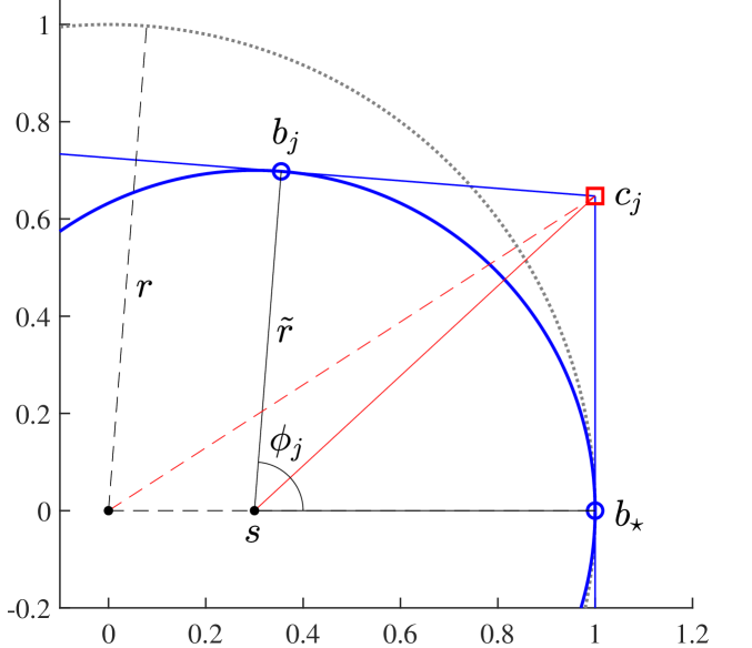
(a) Iteration $j$.

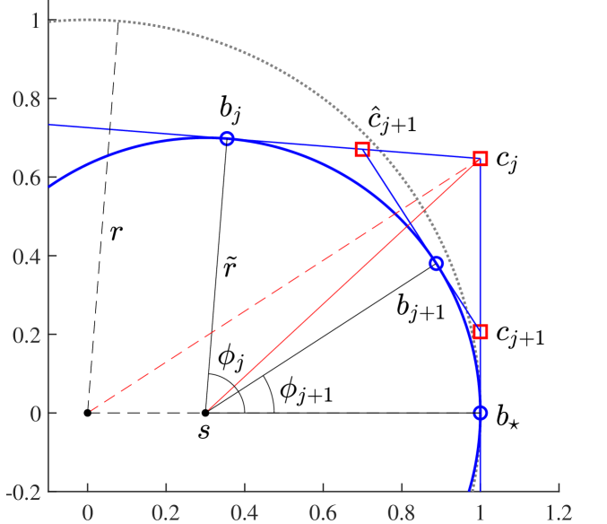
(b) Iteration $j+1$.

Figure 2: Depiction of Uhlig’s cutting procedure on Example 4.6 where $z=0.3$ and $\tilde{r}=0.7$. The dotted circle is the circle of radius $r(M)=1$ centered at the origin. See Example 4.6 for a complete description of the plots.

Example 4.6 (See Fig. 2 for a visual description).

For $n\geq 2$, let

$$M=sI+\tilde{r}K_{n},$$ (4.2)

where $K_{n}\in\mathbb{C}^{n\times n}$ is any disk matrix with $r(K_{n})=1$, e.g., (4.1), $s\geq 0$, and $\tilde{r}>0$. Clearly, $W(M)$ is a disk with radius $\tilde{r}$ centered at $s$ on the real axis with outermost point $b_{\star}=s+\tilde{r}=r$ and $\mu=\tfrac{\tilde{r}}{r}>0$ at $b_{\star}$, where $r\coloneqq r(M)$, a shorthand we will often use in Section 4 and Section 5. Thus, given any matrix $A$ satisfying Assumptions 4.3 and 4.4 with any $\mu\in(0,1]$, by choosing $s\geq 0$ and $\tilde{r}>0$ appropriately we have that $\partial W(M)$ agrees exactly with the osculating circle of $\partial W(A)$ at $b_{\star}$. Assume that $\theta_{\star}=0$ and $\theta_{j}\in(-\pi,0)$ have been used to construct $\mathcal{G}_{j}$ and $\mathcal{Z}_{j}$, i.e., supporting hyperplanes $L_{\theta_{\star}}$ and $L_{\theta_{j}}$ respectively pass through boundary points $b_{\star}$ and $b_{j}=s+\tilde{r}\mathrm{e}^{\mathbf{i}\phi_{j}}$ of $W(M)$, where $\phi_{j}\coloneqq\operatorname{Arg}(b_{j}-s)\in(0,\pi)$. Therefore, $b_{\star}=z_{0}\in\mathcal{Z}_{j}$ and since $W(M)$ is a disk, it also follows that $b_{j}=z_{\theta_{j}}\in\mathcal{Z}_{j}$, where $\theta_{j}=-\phi_{j}$. Further assume that for all $\theta\in(\theta_{j},\theta_{\star})$, $z_{\theta}\not\in\mathcal{Z}_{j}$, and so $c_{j}\coloneqq L_{\theta_{\star}}\cap L_{\theta_{j}}$ is a corner of $\mathcal{G}_{j}$. Now suppose $c_{j}$ is cut, by any cutting procedure, Uhlig’s or otherwise. This results in a boundary point $b_{j+1}$ of $W(M)$ being added to $\mathcal{Z}_{j}$ and $c_{j}$ is replaced by two new corners, $\hat{c}_{j+1}$ and $c_{j+1}$, that respectively lie on $L_{\theta_{j}}$ and $L_{\theta_{\star}}$; due to their orientation with respect to $b_{j+1}$, we refer to $\hat{c}_{j+1}$ as a counter-clockwise (CCW) corner and $c_{j+1}$ as a clockwise (CW) corner. If $c_{j+1}$ is then cut next, this produces two more corners, $\hat{c}_{j+2}$ and $c_{j+2}$, with $c_{j+2}$ also on $L_{\theta_{\star}}$ and between $c_{j+1}$ and $b_{\star}$. Note that if $\{\phi_{k}\}\to 0$, then the sequence of CW corners $\{c_{k}\}=c_{j},c_{j+1},c_{j+2},\ldots$ converges to $b_{\star}$. To understand the local behavior of a cutting-plane technique, we will analyze $\{\phi_{k}\}$ and $\{c_{k}\}$, i.e., the case when the cuts are applied to the CW corners that are sequentially generated on $L_{\theta_{\star}}$.

Some remarks on Example 4.6 are in order, as it ignores the CCW corners $\hat{c}_{j}$, and cutting these CCW corners may also introduce new corners that need to be cut. However, since $\{c_{k}\}$ is a subsequence of all the corners generated by Uhlig’s method to sufficiently approximate $\partial W(M)$ between boundary points $b_{\star}$ and $b_{j}$, analyzing $\{c_{k}\}$ gives a lower bound on its local efficiency. Furthermore, this often describes the true local efficiency because, as will become clear, for many problems, there are either no or few CCW corners that requiring cutting. Finally, in Section 5, we introduce an improved cutting scheme that guarantees only CW corners must be cut.

Lemma 4.7.

Recalling that $\phi_{j}\coloneqq\operatorname{Arg}(b_{j}-s)$, if Uhlig’s cuts are sequentially applied to the corners $\{c_{k}\}$ described in Example 4.6, then for all $k\geq j$,

$$\phi_{k+1}=\arctan\big{(}\mu\tan\tfrac{1}{2}\phi_{k}\big{)}.$$ (4.3)

Proof.

Since $W(M)$ is a disk with tangents at $b_{k}$ and $b_{\star}$ determining $c_{k}$, first note that we have that $\operatorname{Arg}(c_{k}-s)=\tfrac{1}{2}\phi_{k}$. Then $\tan\tfrac{1}{2}\phi_{k}=\tilde{r}^{-1}|c_{k}-b_{\star}|$, and since the tangent at $b_{\star}$ is vertical, we also have that $\operatorname{Arg}(c_{k})=\arctan(r^{-1}|c_{k}-b_{\star}|)$. Thus via substitution,

$$\operatorname{Arg}(c_{k})=\arctan(r^{-1}\tilde{r}\tan\tfrac{1}{2}\phi_{k})=\arctan(\mu\tan\tfrac{1}{2}\phi_{k}).$$

The proof is completed since $\phi_{k+1}=\operatorname{Arg}(b_{k+1}-s)$ is also equal to $\operatorname{Arg}(c_{k})$. ∎

Theorem 4.8.

The sequence $\{\phi_{k}\}$ produced by Uhlig’s cutting procedure and described by recursion (4.3) converges to zero Q-linearly with rate $\tfrac{1}{2}\mu$.

Proof.

First note that $\lim_{k\to\infty}\phi_{k}=0=\phi_{\star}$ and $\phi_{k}>0$ for all $k\geq j$. Then

$$\lim_{k\to\infty}\frac{|\phi_{k+1}-\phi_{\star}|}{|\phi_{k}-\phi_{\star}|}=\lim_{k\to\infty}\frac{\phi_{k+1}}{\phi_{k}}=\lim_{k\to\infty}\frac{\arctan\left(\mu\tan\tfrac{1}{2}\phi_{k}\right)}{\phi_{k}}.$$

Since the numerator and denominator both go to zero as $k\to\infty$, the result follows by considering the continuous version of the limit:

$$\lim_{\phi\to 0}\frac{\arctan\big{(}\mu\tan\tfrac{\phi}{2}\big{)}}{\phi}=\lim_{\phi\to 0}\frac{\mu\tan\tfrac{1}{2}\phi}{\phi}=\lim_{\phi\to 0}\frac{\tfrac{1}{2}\mu\phi}{\phi}=\tfrac{1}{2}\mu,$$

where the first and second equalities are obtained, respectively, using small-angle approximations $\arctan x\approx x$ and $\tan x\approx x$ for $x\approx 0$. ∎

While Theorem 4.8 tells us how quickly $\{\phi_{k}\}$ will converge, we really want to estimate how quickly the error $\varepsilon_{j}$ becomes sufficiently small. For that, we must consider how fast the moduli of the corresponding outermost corners $c_{k}$ converge.

Theorem 4.9.

Given the sequence $\{\phi_{k}\}$ from Theorem 4.8, the corresponding sequence $\{|c_{k}|\}$ converges to $r$ Q-linearly with rate $\tfrac{1}{4}\mu^{2}$.

Proof.

First note that

$$\cos\phi_{k+1}=\frac{r}{|c_{k}|}\qquad\text{and so}\qquad|c_{k}|=r\sec\phi_{k+1}>r$$

for all $k\geq j$. Thus, we consider the limit

$$\lim_{k\to\infty}\frac{||c_{k+1}|-r|}{||c_{k}|-r|}=\lim_{k\to\infty}\frac{r\sec\phi_{k+2}-r}{r\sec\phi_{k+1}-r}=\lim_{k\to\infty}\frac{\sec\phi_{k+1}-1}{\sec\phi_{k}-1},$$

which when substituting in $\phi_{k+1}=\arctan\big{(}\mu\tan\tfrac{1}{2}\phi_{k}\big{)}$ becomes

$$\lim_{k\to\infty}\frac{\sec\left(\arctan\left(\mu\tan\tfrac{1}{2}\phi_{k}\right)\right)-1}{\sec\phi_{k}-1}.$$

Since the numerator and denominator both go to zero as $k\to\infty$, we consider the continuous version of the limit, i.e.,

$$\lim_{\phi\to 0}\frac{\sec\left(\arctan\left(\mu\tan\tfrac{1}{2}\phi\right)\right)-1}{\sec\phi-1}=\lim_{\phi\to 0}\frac{\sec\left(\mu\tan\tfrac{1}{2}\phi\right)-1}{\sec\phi-1}=\lim_{\phi\to 0}\frac{\sec\left(\tfrac{1}{2}\mu\phi\right)-1}{\sec\phi-1},$$

again using the small-angle approximations for $\arctan$ and $\tan$. Letting $g(\phi)=\sec(\phi)$, and noting that $g(0)=1$, $g^{\prime}(0)=0$, and $g^{\prime\prime}(0)=1$, its Taylor expansion about $0$ is

$$g(\phi)=1+\tfrac{1}{2}\phi^{2}+\sum_{n=3}^{\infty}\frac{g^{(n)}(0)}{n!}\phi^{n}.$$

Replacing the secant terms in both the numerator and denominator of the limit above with their Taylor expansions, we obtain the equivalent limit yielding our result:

$$\lim_{\phi\to 0}\frac{\tfrac{1}{2}(\tfrac{1}{2}\mu\phi)^{2}+\mathcal{O}(\phi^{3})}{\tfrac{1}{2}\phi^{2}+\mathcal{O}(\phi^{3})}=\tfrac{1}{4}\mu^{2}.$$

∎

As Example 4.6 can model any $\mu\in(0,1]$, per 4.5, Theorems 4.8 and 4.9 also accurately describe the local behavior of Uhlig’s cutting procedure at outermost points in $W(A)$ for any matrix $A$. Moreover, due to the squaring and one-quarter factor in Theorem 4.9, the linear rate of convergence becomes very fast rather rapidly as $\mu$ decreases from one, ultimately becoming superlinear if the outermost point is a corner ($\mu=0$). We can also estimate the cost of approximating $\partial W(A)$ about $b_{\star}$, determining how many iterations will be needed until it is no longer necessary to refine corner $c_{k}$, i.e., the value of $k$ such that $|c_{k}|\leq r(A)\cdot(1+\tau_{\mathrm{tol}})$. For simplicity, it will now be more convenient to assume that $j=0$ with $|c_{0}|=\beta r(A)$ for some scalar $\beta>(1+\tau_{\mathrm{tol}})$. Via the Q-linear rate given by Theorem 4.9, we have that

$$|c_{k}|-r(A)\leq(|c_{0}|-r(A))\cdot\left(\tfrac{1}{4}\mu^{2}\right)^{k},$$

and so if

$$r(A)+(|c_{0}|-r(A))\cdot\left(\tfrac{1}{4}\mu^{2}\right)^{k}\leq r(A)\cdot(1+\tau_{\mathrm{tol}}),$$

then it follows that $|c_{k}|\leq r(A)\cdot(1+\tau_{\mathrm{tol}})$, i.e., it does not need to be refined further. By first dividing the above equation by $r(A)$ and doing some simple manipulations, we have that $|c_{k}|$ is indeed sufficiently close to $r(A)$ if

$$k\geq\frac{\log(\tau_{\mathrm{tol}})-\log(\beta-1)}{\log\left(\tfrac{1}{4}\mu^{2}\right)}.$$ (4.4)

Using Example 4.6 with $\beta=100$, and $\tau_{\mathrm{tol}}=\texttt{1e-14}$, only $k\approx 27$, $14$, $7$, and $4$ iterations are needed, respectively, for $\mu=1$, $0.5$, $0.1$, and $0.01$. This is indeed rather fast for linear convergence. Of course, if $W(A)$ has more than one outermost point, the total cost of a cutting-plane method increases commensurately, since $\partial W(A)$ must be well approximated about all of these outermost points. For disk matrices, all boundary points are outermost, and so the cost blows up, per Theorem 4.1.

5 An improved cutting-plane algorithm

We now address some inefficiencies in Uhlig’s method by giving an improved cutting-plane method. The two main components of this refined algorithm are as follows. First, any of the local optimization techniques from Section 3 also allows us to more efficiently locate outermost points in $W(A)$. This is possible because each outermost point is bracketed on $\partial W(A)$ by two boundary points of $W(A)$ in $\mathcal{Z}_{j}$, and these brackets improve as $\mathcal{G}_{j}$ more accurately approximates $W(A)$. Therefore, once $\mathcal{G}_{j}$ is no longer a crude approximation, these brackets can be used to initialize optimization to find global maximizers of $h(\theta)$, and thus, globally outermost points of $W(A)$. Second, given a boundary point of $W(A)$ that is also known to be locally outermost, we use a new cutting procedure that reduces the total number of cuts needed to sufficiently approximate $\partial W(A)$ in this region. When this new cut cannot be invoked, we will fall back on Uhlig’s cutting procedure. In the next three subsections, we describe our new cutting strategy, establish a Q-linear rate of convergence for it, and finally, show how these cuts can be sufficiently well estimated so that our theoretical convergence rate result is indeed realized in practice. Finally, pseudocode of our completed algorithm is given in Algorithm 5.1.

5.1 An optimal-cut strategy

Again consider Example 4.6. In Fig. 2b, Uhlig’s cut of corner $c_{j}$ between $b_{j}$ (with $|b_{j}|<r$) and $b_{\star}$ produces two new corners $\hat{c}_{j+1}$ and $c_{j+1}$, but since $|\hat{c}_{j+1}|<r$ and $|c_{j+1}|>r$, it is only necessary to subsequently refine $c_{j+1}$. However, in Fig. 3a we show another scenario where both of the two new corners produced by Uhlig’s cut will require subsequent cutting as well. While Theorems 4.8 and 4.9 indicate the number of iterations Uhlig’s method needs to sufficiently refine the sequence $\{c_{k}\}$, they do not take into account that the CCW corners that are generated may also need to be cut. Thus, the total number of eigenvalue computations with $H(\theta)$ can be higher than what is suggested by these two theorems. However, comparing Figs. 2b and 3a immediately suggests a better strategy, namely, to make the largest reduction in the angle $\phi_{j}$ such that the CCW corner $\hat{c}_{j+1}$ (between $b_{j}$ and $c_{j}$ on the tangent line for $b_{j}$) does not subsequently need to be refined, i.e., such that $|\hat{c}_{j+1}|=r$. In Fig. 3a, this ideal corner is labeled $d_{j}$, while the corresponding optimal cut for this same example is shown in Fig. 3b, where $d_{j}$ coincides with $\hat{c}_{j+1}$, and so the latter is not labeled.

5.2 Convergence analysis of the optimal cut

Before describing how to compute optimal cuts, we derive the convergence rate of the sequence of angles $\{\phi_{k}\}$ this strategy produces. Per 4.5, it again suffices to study Example 4.6.

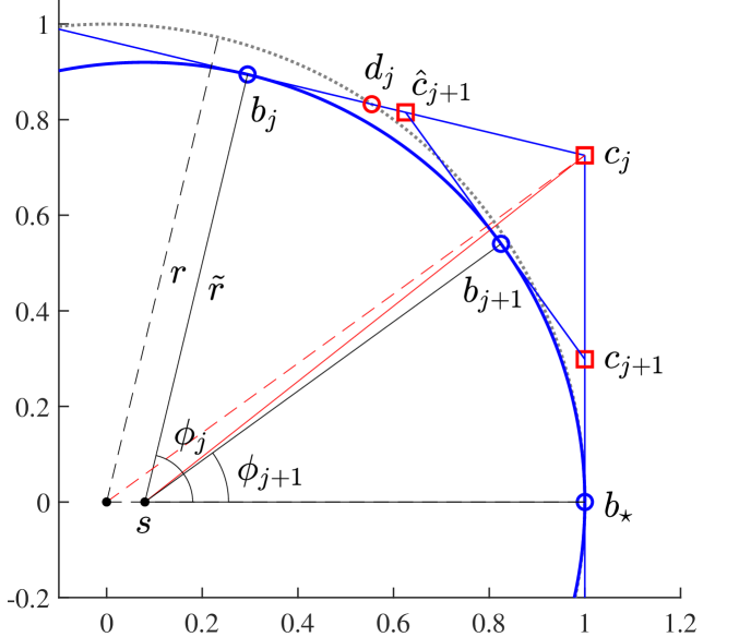
(a) Uhlig’s cut.

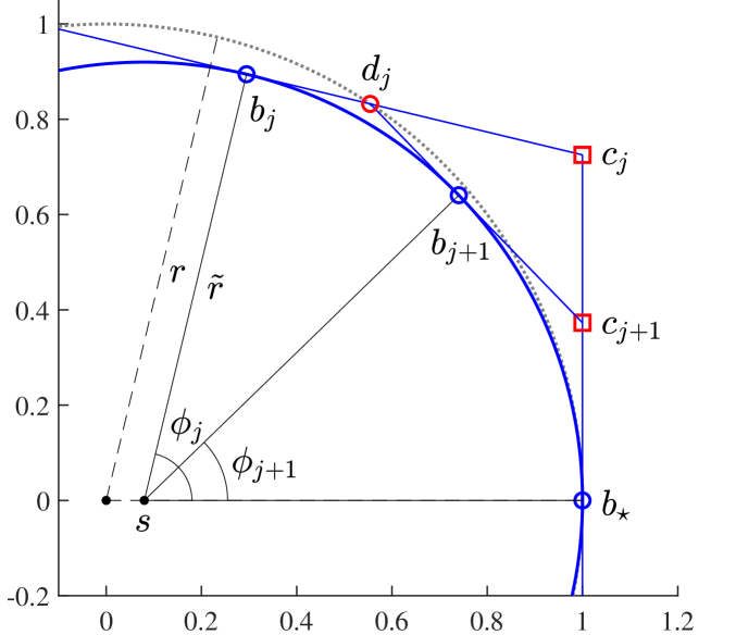
(b) The optimal cut.

Figure 3: Depictions of corner $c_{j}$ between boundary points $b_{j}$ and $b_{\star}$ being cut by Uhlig’s cutting procedure (left) and the optimal cut (right), where the latter always makes the largest possible reduction in $\phi_{j}$ such that only corner $c_{j+1}$ must be refined.

Lemma 5.1.

Given Example 4.6, additionally assume that $|b_{j}|<r$ and $\tilde{r}<r$, and so at $b_{\star}$, $\mu\in(0,1)$. Then the point on $L_{\theta_{j}}$, i.e., the supporting hyperplane passing through $b_{j}$ where $\theta_{j}=-\phi_{j}\in(-\pi,0)$, that is closest to $c_{j}$ and has modulus $r$ is

$$d_{j} =b_{j}-\mathbf{i}t_{j}\mathrm{e}^{\mathbf{i}\phi_{j}},\quad\text{where}$$ (5.1a)

$$t_{j} =-s\sin\phi_{j}+\sqrt{s^{2}\sin^{2}\phi_{j}+2s\tilde{r}(1-\cos\phi_{j})}>0.$$ (5.1b)

Proof.

As $\phi_{j}\in(0,\pi)$, clearly (5.1a) must hold for some $t_{j}>0$. To obtain (5.1b), we use the fact that $|d_{j}|^{2}=r^{2}$ and solve for $t_{j}$ using (5.1a). Setting $u=\mathrm{e}^{\mathbf{i}\phi_{j}}$, we have

$$0 =|d_{j}|^{2}-r^{2}=(b_{j}-\mathbf{i}t_{j}u)\big{(}\overline{b}_{j}+\mathbf{i}t_{j}\overline{u})-r^{2}=t_{j}^{2}+\mathbf{i}(b_{j}\overline{u}-\overline{b}_{j}u)t_{j}+|b_{j}|^{2}-r^{2}.$$

which by substituting in the following two equivalences

$$b_{j}\overline{u}-\overline{b}_{j}u =(s+\tilde{r}u)\overline{u}-(s+\tilde{r}\overline{u})u=s(\overline{u}-u)=-\mathbf{i}2s\sin\phi_{j},$$

$$|b_{j}|^{2} =s^{2}+\tilde{r}^{2}+s\tilde{r}(u+\overline{u})=s^{2}+\tilde{r}^{2}+2s\tilde{r}\cos\phi_{j},$$

yields

$$0=t_{j}^{2}+(2s\sin\phi_{j})t_{j}+(s^{2}+\tilde{r}^{2}-r^{2}+2s\tilde{r}\cos\phi_{j}).$$

By substituting in $r^{2}=(s+\tilde{r})^{2}=s^{2}+\tilde{r}^{2}+2s\tilde{r}$, this simplifies further to

$$0=t_{j}^{2}+(2s\sin\phi_{j})t_{j}+2s\tilde{r}(\cos\phi_{j}-1).$$

Thus, by the quadratic formula, we obtain (5.1b). ∎

Lemma 5.2.

Given the assumptions in Lemma 5.1 and $t_{j}>0$ from (5.1b), also suppose that $\phi_{j}\in(0,\tfrac{\pi}{2})$. Then if optimal cuts are sequentially applied to the corners $\{c_{k}\}$ described in Example 4.6, for all $k\geq j$,

$$\phi_{k+1}=-\phi_{k}+2\arctan\left(\frac{\tilde{r}\sin\phi_{k}-t_{k}\cos\phi_{k}}{\tilde{r}\cos\phi_{k}+t_{k}\sin\phi_{k}}\right).$$ (5.2)

Proof.

Let $\hat{\phi}=\phi_{k}-\operatorname{Arg}(d_{k}-s)$. Then it follows that

$$\phi_{k+1}=\phi_{k}-2\hat{\phi}=-\phi_{k}+2\operatorname{Arg}(d_{k}-s)=-\phi_{k}+2\arctan\left(\frac{\mathrm{Im}\,(d_{k}-s)}{\mathrm{Re}\,(d_{k}-s)}\right),$$ (5.3)

where the last equality follows because $\mathrm{Re}\,(d_{k}-s)>0$, as $\mathrm{Re}\,b_{k}>s$. Using (5.1a) and substituting in $b_{k}=s+\tilde{r}\mathrm{e}^{\mathbf{i}\phi_{k}}$, we have that

$$d_{k}-s=\tilde{r}\mathrm{e}^{\mathbf{i}\phi_{k}}-\mathbf{i}t_{k}\mathrm{e}^{\mathbf{i}\phi_{k}}\qquad\Longleftrightarrow\qquad\begin{aligned} \mathrm{Re}\,(d_{k}-s)&=\tilde{r}\cos\phi_{k}+t_{k}\sin\phi_{k},\\ \mathrm{Im}\,(d_{k}-s)&=\tilde{r}\sin\phi_{k}-t_{k}\cos\phi_{k}.\end{aligned}$$

Substituting these into (5.3) completes the proof. ∎

Before deriving how fast $\{\phi_{k}\}$ converges, we show that it indeed converges to zero.

Lemma 5.3.

Given the assumptions of Lemma 5.2, the recursion (5.2) for optimal cuts produces a sequence of angles $\{\phi_{k}\}$ converging to zero.

Proof.

By construction, $\{\phi_{k}\}$ is monotone, i.e., $\phi_{k+1}<\phi_{k}$ for all $k\geq j$, and bounded below by zero, and so $\{\phi_{k}\}$ converges to some limit $l$. Per (5.1b), the $t_{k}$ values appearing in (5.2) depend on $\phi_{k}$, so we define the analogous continuous function

$$t(\phi)=-s\sin\phi+\sqrt{s^{2}\sin^{2}\phi+2s\tilde{r}(1-\cos\phi)}.$$ (5.4)

Now by way of contradiction, assume that $l>0$ and so $0<l<\phi_{j}<\tfrac{\pi}{2}$. Thus,

$$\lim_{k\to\infty}\phi_{k+1}=l=-l+2\arctan\left(\frac{\tilde{r}\sin l-t(l)\cos l}{\tilde{r}\cos l+t(l)\sin l}\right)\ \Leftrightarrow\ \tan l=\frac{\tilde{r}\sin l-t(l)\cos l}{\tilde{r}\cos l+t(l)\sin l}.$$

Then, by multiplying both sides by $\tilde{r}\cos l+t(l)\sin l$ and rearranging terms, we obtain the equality $t(l)(\sin^{2}l+\cos^{2}l)=0$, and so $t(l)=0$. However, Lemma 5.1 states that $t(l)>0$ should hold since $l\in(0,\tfrac{\pi}{2})$, a contradiction, and so $l=0$. ∎

We now have the necessary pieces to derive the exact rate of convergence of the angles produced by optimal cuts.

Theorem 5.4.

The sequence $\{\phi_{k}\}$ produced by optimal cuts and described by recursion (5.2) converges to zero Q-linearly with rate $\tfrac{2(1-\sqrt{1-\mu})}{\mu}-1$.

Proof.

By Lemmas 5.2 and 5.3, (5.2) holds, $\phi_{k}\to\phi_{\star}=0$, and $\phi_{k}\geq 0$ for all $k\geq j$, so

$$\lim_{k\to\infty}\frac{|\phi_{k+1}-\phi_{\star}|}{|\phi_{k}-\phi_{\star}|}=\lim_{k\to\infty}\frac{\phi_{k+1}}{\phi_{k}}=\lim_{k\to\infty}\frac{-\phi_{k}+2\arctan\left(\frac{\tilde{r}\sin\phi_{k}-t_{k}\cos\phi_{k}}{\tilde{r}\cos\phi_{k}+t_{k}\sin\phi_{k}}\right)}{\phi_{k}}.$$

Using the continuous version of $t_{k}$ given in (5.4), we instead consider the entire limit in continuous form:

$$\lim_{\phi\to 0}\frac{-\phi+2\arctan\left(\frac{\tilde{r}\sin\phi-t(\phi)\cos\phi}{\tilde{r}\cos\phi+t(\phi)\sin\phi}\right)}{\phi}=-1+\lim_{\phi\to 0}\frac{2}{\phi}\cdot\frac{\tilde{r}\phi-t(\phi)\cos\phi}{\tilde{r}\cos\phi+t(\phi)\phi},$$ (5.5)

where the equality holds by using the small-angle approximations $\arctan x\approx x$ (as the ratio inside the $\arctan$ above goes to zero as $\phi\to 0$) and $\sin x\approx x$. Again using $\sin x\approx x$ as well as the small-angle approximation $1-\cos x\approx\tfrac{1}{2}x^{2}$, we also have the small-angle approximation

$$t(\phi)\approx-s\phi+\sqrt{s^{2}\phi^{2}+2s\tilde{r}\big{(}\tfrac{1}{2}\phi^{2}\big{)}}=-\phi\left(s-\phi\sqrt{s^{2}+s\tilde{r}}\right)=-\phi\left(s-\sqrt{sr}\right),$$ (5.6)

where the last equality holds since $\tilde{r}=r-s$. Via substituting in (5.6), the limit on the right-hand side of (5.5) is

$$\lim_{\phi\to 0}\frac{2}{\phi}\cdot\frac{\tilde{r}\phi+\phi\left(s-\sqrt{sr}\right)\cos\phi}{\tilde{r}\cos\phi-\phi\left(s-\sqrt{sr}\right)\phi}=\lim_{\phi\to 0}\frac{2\left(\tilde{r}+\left(s-\sqrt{sr}\right)\cos\phi\right)}{\tilde{r}\cos\phi-\phi^{2}\left(s-\sqrt{sr}\right)}\\ =\frac{2\left(\tilde{r}+s-\sqrt{sr}\right)}{\tilde{r}}.$$

Recalling that $\tilde{r}=\mu r$ and that $s=r-\tilde{r}=r-\mu r$, by substitutions we can rewrite the ratio above as

$$\frac{2\left(\mu r+(r-\mu r)-\sqrt{(r-\mu r)r}\right)}{\mu r}=\frac{2\left(r-r\sqrt{1-\mu}\right)}{\mu r}=\frac{2\left(1-\sqrt{1-\mu}\right)}{\mu}.$$

Subtracting one from the value above completes the proof. ∎

As we show momentarily, optimal cuts have a total lower cost than Uhlig’s cutting procedure. Thus, there is no need to derive an analogue of Theorem 4.9 for describing the convergence rate of the moduli of corners $c_{k}$ produced by the optimal-cut strategy.

5.3 Computing the optimal cut

Suppose that $b_{\star}\in\mathcal{Z}_{j}$ attains the value of $l_{j}$, and that $b_{\star}$ is also locally outermost in $W(A)$, and let $\gamma=|b_{\star}|\leq r(A)$. Without loss of generality, we assume that $\operatorname{Arg}(b_{\star})=0$, and let $b_{j}\in\mathcal{Z}_{j}$ be the next known boundary point of $W(A)$ with $\operatorname{Arg}(b_{j})\in(0,\pi)$. We can model $\partial W(A)$ between $b_{\star}$ and $b_{j}$ by fitting a quadratic that interpolates $\partial W(A)$ at $b_{\star}$ and $b_{j}$. If this model is a good fit, then it can be used to estimate $d_{j}$, and thus, also the optimal cut.

Since $b_{\star}$ is also a locally outermost point of $W(A)$ and $\operatorname{Arg}(b_{\star})=0$, we can interpolate these boundary points using the sideways quadratic (opening up to the left in the complex plane)

$$q(y)=q_{2}y^{2}+q_{1}y+q_{0},$$

with the remaining degree of freedom used to specify that $q(y)$ should be tangent to $W(A)$ at $b_{\star}$. Clearly, $q(y)$ cannot be a good fit if $L_{\theta_{j}}$, the supporting hyperplane passing through $b_{j}$, is increasing from left to right in the complex plane; hence, we also assume that $\theta_{j}\in(-\tfrac{\pi}{2},0)$. Let $\theta_{\dagger}\in(\theta_{j},0)$ denote the angle of the supporting hyperplane for the optimal cut, e.g., for Example 4.6, the one that passes through $d_{j}$ and the boundary point $b_{j+1}$ between $b_{j}$ and $b_{\star}$. By our criteria, the equations

$$q(0)=\gamma,\quad q(\mathrm{Im}\,b_{j})=\mathrm{Re}\,b_{j},\quad\text{and}\quad q^{\prime}(0)=0$$ (5.7)

determine the coefficients $q_{0}$, $q_{1}$, and $q_{2}$, and solving these yields

$$q_{2}=\frac{\mathrm{Re}\,b_{j}-\gamma}{(\mathrm{Im}\,b_{j})^{2}},\quad q_{1}=0,\quad\text{and}\quad q_{0}=\gamma.$$ (5.8)

Algorithm 5.1 An Improved Cutting-Plane Algorithm

0:   $A\in\mathbb{C}^{n\times n}$ with $n\geq 2$ and $\tau_{\mathrm{tol}}>0$.

0:   $l$ such that $|l-r(A)|\leq\tau_{\mathrm{tol}}\cdot r(A)$.  

1:  $\mathcal{G}\leftarrow P_{\theta_{1}}\cap\cdots\cap P_{\theta_{4}}$ where $\theta_{\ell}=\tfrac{\ell-1}{2}\pi$ for $\ell=1,2,3,4$

2:  $\mathcal{Z}\leftarrow\{z_{\theta_{\ell}}:\ell=1,2,3,4\}$

3:  $l\leftarrow\max\{|b|:b\in\mathcal{Z}\}$, $u\leftarrow\max\{|c|:c\text{ a corner of }\mathcal{G}\}$

4:  while $\tfrac{u-l}{l}>\tau_{\mathrm{tol}}$  do

5:     $L_{\theta_{1}}\leftarrow$ supporting hyperplane for the boundary point in $\mathcal{Z}$ attaining $l$

6:     $\gamma\leftarrow$ local max of $\rho(H(\theta))$ via optimization initialized at $\theta_{1}$

7:     $\mathcal{G}\leftarrow\mathcal{G}\cap P_{\theta_{1}}\cap\cdots\cap P_{\theta_{q}}$ for the $q$ angles $\theta_{\ell}$ encountered during optimization

8:     $\mathcal{Z}\leftarrow\mathcal{Z}\cup\{z_{\theta_{\ell}}:\ell=1,\ldots,q\}$

9:     $c\leftarrow\text{ outermost corner of }\mathcal{G}$

10:     if  the optimal cut should be applied to $c$ per Section 5.3  then

11:        $\theta\leftarrow$ angle $\theta_{\dagger}$ is given by (5.12) (rotated and flipped as necessary)

12:     else

13:        $\theta\leftarrow-\operatorname{Arg}(c)$ // Uhlig’s cut

14:     end if

15:     $\mathcal{G}\leftarrow\mathcal{G}\cap P_{\theta}$

16:     $\mathcal{Z}\leftarrow\mathcal{Z}\cup\{z_{\theta}\}$

17:     $l\leftarrow\max\{|b|:b\in\mathcal{Z}\}$, $u\leftarrow\max\{|c|:c\text{ a corner of }\mathcal{G}\}$

18:  end while

Note: For simplicity, we forgo describing pseudocode to exploit possible normality of $A$ or symmetry of $W(A)$, and assume that $A\neq 0$, eigenvalues and local maximizers are obtained exactly, optimization is monotonic, i.e., $l\leq\gamma$ is guaranteed, and there are no ties for the boundary point in line 5.

We can assess whether $q(y)$ is a good fit for $\partial W(A)$ about $b_{\star}$ by checking how close $q(y)$ is to being tangent to $\partial W(A)$ at $b_{j}$, i.e., $q(y)$ is a good fit if

$$q^{\prime}(\mathrm{Im}\,b_{j})\approx\tan\theta_{j}.$$ (5.9)

If these two values are not sufficiently close, then we consider $q(y)$ a poor local approximation of $\partial W(A)$ at $b_{j}$ (and $b_{\star}$) and use Uhlig’s cutting procedure to update $\mathcal{G}_{j}$ and $\mathcal{Z}_{j}$. Otherwise, we assume that $q(y)$ does accurately model $\partial W(A)$ in this region and do an optimal cut. To estimate $\theta_{\dagger}$, we need to determine the line

$$a(y)=a_{1}y+a_{0}$$

such that $a(y)$ passes through $d_{j}$ for $y=\mathrm{Im}\,d_{j}$ and is tangent to $q(y)$ for some $\tilde{y}\in(0,\mathrm{Im}\,d_{j})$. Thus, we solve the following set of equations:

$$\mathrm{Re}\,d_{j} =a(\mathrm{Im}\,d_{j}) \qquad\Longleftrightarrow\qquad \mathrm{Re}\,d_{j} =a_{1}\mathrm{Im}\,d_{j}+a_{0},$$ (5.10a)

$$q(\tilde{y}) =a(\tilde{y}) \qquad\Longleftrightarrow\qquad q_{2}\tilde{y}^{2}+q_{0} =a_{1}\tilde{y}+a_{0},$$ (5.10b)

$$q^{\prime}(\tilde{y}) =a^{\prime}(\tilde{y}) \qquad\Longleftrightarrow\qquad 2q_{2}\tilde{y} =a_{1},$$ (5.10c)

to determine $a_{0}$, $a_{1}$ and $\tilde{y}$. This yields

$$\tilde{y}=\mathrm{Im}\,d_{j}-\sqrt{(\mathrm{Im}\,d_{j})^{2}+\tfrac{q_{0}-\mathrm{Re}\,d_{j}}{q_{2}}},\ \ \ a_{0}=-q_{2}\tilde{y}^{2}+q_{0},\ \ \ \text{and}\ \ \ a_{1}=\frac{\mathrm{Re}\,d_{j}-a_{0}}{\mathrm{Im}\,d_{j}},$$ (5.11)

where $a_{1}$ follows directly from (5.10a), $a_{0}$ is obtained by substituting the value of $a_{1}$ given in (5.10c) into (5.10b), and $\tilde{y}$ follows from substituting the value of $a_{0}$ given in (5.11) into $a_{1}$ in (5.11) (so that $a_{1}$ now only has $\tilde{y}$ as an unknown), and then substituting this version of $a_{1}$ into (5.10c), which results in a quadratic equation in $\tilde{y}$. Since $q(y)$ is a sufficiently accurate local model of $\partial W(A)$, it follows that

$$\theta_{\dagger}\approx\arctan a_{1}.$$ (5.12)

If $\gamma=r(A)$, we can also estimate the value of $\mu$ at $b_{\star}$ via

$$\mu_{\mathrm{est}}\coloneqq\frac{1}{2|q_{2}|\gamma},$$ (5.13)

as the osculating circle of $q(y)$ at $y=0$ has radius $\tfrac{1}{2}|q_{2}|$. While the value of $\mu$ at $b_{\star}$ might be computed using Theorem 2.3, this would be much more expensive and it requires that $\lambda_{\mathrm{max}}(H(0))$ be simple, which may not hold. Detecting the normalized radius of curvature at outermost points via (5.13) will be a key component of our hybrid algorithm in Section 6.

Our formulas for computing $\theta_{\dagger}$ can be used for any outermost point simply by rotating and flipping the problem as necessary to satisfy the assumptions on $b_{\star}$ and $b_{j}$. To be robust against even small rounding errors, instead of $d_{j}$, we use $(1-\delta)d_{j}+\delta b_{j}$ for some small $\delta\in(0,1)$, i.e., a point slightly closer to $b_{j}$.

For different values of $\mu\in[0,1)$, Fig. 4a plots the convergence rates for $\{\phi_{k}\}$ given by Theorems 4.8 and 5.4, while Fig. 4b shows the total number of cuts needed by each cutting strategy in order to sufficiently approximate $\partial W(M)$ near $b_{\star}$. Uhlig’s method is usually slightly more expensive but becomes significantly worse than optimal cutting for normalized curvatures $\mu\approx 0.84$ and higher, requiring about double the number of cuts at this transition point. A variant of Fig. 4b (not shown) also reveals that optimal cuts become slightly more expensive than Uhlig’s cuts for $\mu\approx 0.999961$ and above, and so we only use the optimal cut when $\mu_{\mathrm{est}}$ is less than this value.

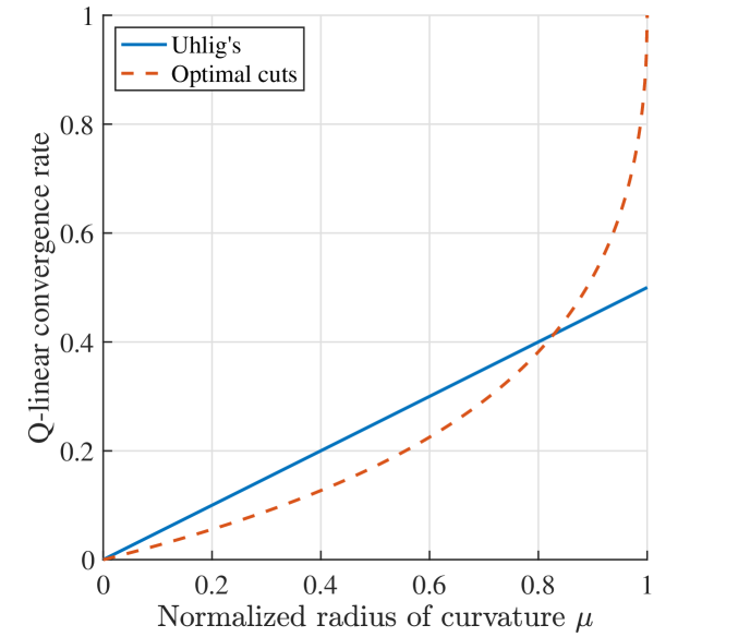
(a) Convergence rates of $\{\phi_{k}\}$.

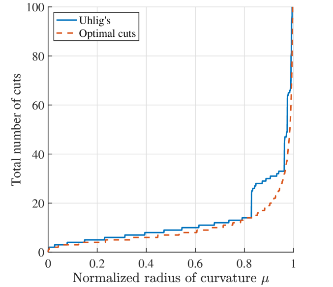
(b) Cost to approximate $\partial W(M)$ region.

Figure 4: Left: the respective convergence rates of $\{\phi_{j}\}$ given by Theorems 4.8 and 5.4. Right: for the parametric matrix $M$ with $\mu\in(0,1]$ given by Example 4.6 and a tolerance $\tau_{\mathrm{tol}}=\texttt{1e-14}$, the total number of cuts required to sufficiently approximate the region of $\partial W(M)$ specified by the supporting hyperplanes $L_{\theta_{\star}}$ and $L_{\theta_{j}}$ respectively passing through $b_{\star}$ and $b_{j}$ and the corner $c_{j}$, where $\theta_{\star}=0$ and $\theta_{j}=-\tfrac{\pi}{50}$.

6 A hybrid algorithm

Table 1 and our new analyses suggest that it would be far more efficient to combine level-set and cutting-plane techniques in a single hybrid algorithm rather than rely on either technique alone. For the smallest values of $n$, the level-set approach would generally be most efficient, while for larger problem sizes, which approach would be fastest depends on the specific shape of $W(A)$ and the normalized radius of curvature at outermost points. While we cannot know these things a priori, per (5.13), Algorithm 5.1 can estimate $\mu$ as it iterates, and so we can predict how many more cuts may be needed about a particular outermost point. The current approximation $\mathcal{G}$ and $\mathcal{Z}$ can also be used to obtain cheaply computed estimates of how many more cuts will be needed to approximate regions of $\partial W(A)$ to sufficient accuracy. Consequently, as Algorithm 5.1 iterates, we can maintain an evolving estimate of how many more cuts would be needed in order to compute $r(A)$ to the desired tolerance. Thus, our hybrid algorithm can automatically determine if the cutting-plane approach is likely to be fast or slow, and if the latter, automatically switch to the level-set approach. For example, in practice, Algorithm 3.1 often only requires one to two eigenvalue computations with $R_{\gamma}-\lambda S$ and several more with $H(\theta)$. Hence, in conjunction with tuning/benchmark data, such as that shown in Table 1, our hybrid algorithm can reliably estimate whether it will be faster to continue Algorithm 5.1 or immediately switch to Algorithm 3.1, which will be warm-started using the angle of the supporting hyperplane that passes through the point in $\mathcal{Z}$ that attains $l$ in line 5 of Algorithm 5.1, as well as the arguments of the corners to the left and right of this point.

7 Numerical validation

Experiments were done in MATLAB R2021a (Update 6) on a 2020 13” MacBook Pro with an Intel i5 1038NG7 quad-core CPU laptop, 16GB of RAM, and macOS v12.4. For each code, the desired relative tolerance was set to $10^{-14}$, and we only report errors when they were greater than this amount. We used eig for all eigenvalue computations as (a) it sufficed to verify the benefits of our new methods and theoretical results and (b) this consistency simplifies the comparisons; e.g., numr, Mengi’s implementation of his level-set method with Overton, also only uses eig. All code and data are included as supplementary material for reproducibility. Implementations of our new methods will also be added to ROSTAPACK [Mit].

We begin by comparing Algorithm 3.1 to numr. Per Table 3, Algorithm 3.1 generally only needed a single eigenvalue computation with $R_{\gamma}-\lambda S$ and at most two, and for $n\geq 300$, ranged from 4.3–6.9 times faster than numr. Even with optimization disabled, our iteration using $\rho(H(\theta))$ was still faster than numr.

Table 3: For dense random $A$ matrices, the costs of Algorithm 3.1 and Mengi’s code numr (MO, for Mengi and Overton’s method) are shown. We tested Algorithm 3.1 with optimization enabled (Opt., done via Newton’s method) and disabled (Mid., for midpoints only).

	# of eig($R_{\gamma}$,$S$)			# of eig($H(\theta)$)			Time (sec.)
	Alg. 3.1		MO	Alg. 3.1		MO	Alg. 3.1		MO
$n$	Opt.	Mid.		Opt.	Mid.		Opt.	Mid.
100	$1$	$4$	6	9	10	39	$0.1$	$0.2$	$0.2$
200	$2$	$4$	5	14	11	34	$0.6$	$1.0$	$1.2$
300	$1$	$4$	5	17	9	26	$1.2$	$3.9$	$4.9$
400	$1$	$5$	7	17	15	42	$2.7$	$11.7$	$16.0$
500	$1$	$3$	7	7	8	54	$4.5$	$12.8$	$30.7$
600	$1$	$4$	7	8	10	45	$7.7$	$28.7$	$51.4$

We now verify that our local convergence rate analyses from Section 4.2 and Section 5.2 do indeed hold for general matrices and that our procedure for computing optimal cuts is sufficiently accurate to realize the convergence rate given by Theorem 5.4. First, we obtained 200 general examples with roughly equally spaced values of $\mu\in[0,1]$. This was done by running optimization on $\min_{X}r(A+BXC)$, where $A\in\mathbb{C}^{10\times 10}$ is diagonal, while $B\in\mathbb{C}^{10\times 5}$, $C\in\mathbb{C}^{5\times 10}$, and $X\in\mathbb{R}^{5\times 5}$ are dense, and collecting the iterates. By starting at $X=0$, we obtain an example with $\mu=0$; since $A$ is diagonal, $W(A)$ is a polygon. Since minimizing $r(A+BXC)$ often causes $\mu\to 1$ as optimization progresses [LO20], we also obtain a sequence of examples $A+BX_{k}C$ for iterates $\{X_{k}\}$ with various $\mu$ values (computed via Theorem 2.3). Generating new $A$, $B$, and $C$ matrices and running optimization from $X_{0}=0$ was repeated in a loop until the desired set of 200 general examples had been obtained. For each problem, we recorded the total number of cuts that Uhlig’s cutting procedure and the optimal-cut strategy needed to sufficiently approximate the field of values boundary in a small neighborhood to one side of the outermost point in its field of values. More specifically, we performed an analogous experiment to the one we showed earlier for approximating a region of the boundary of Example 4.6. As can be seen by comparing Figs. 4b and 5, for any given $\mu$, the total number of cuts needed on arbitrarily shaped fields of values is essentially the same as that needed for Example 4.6, thus validating the generality of our convergence rate analysis and the reliability of our method for computing optimal cuts.

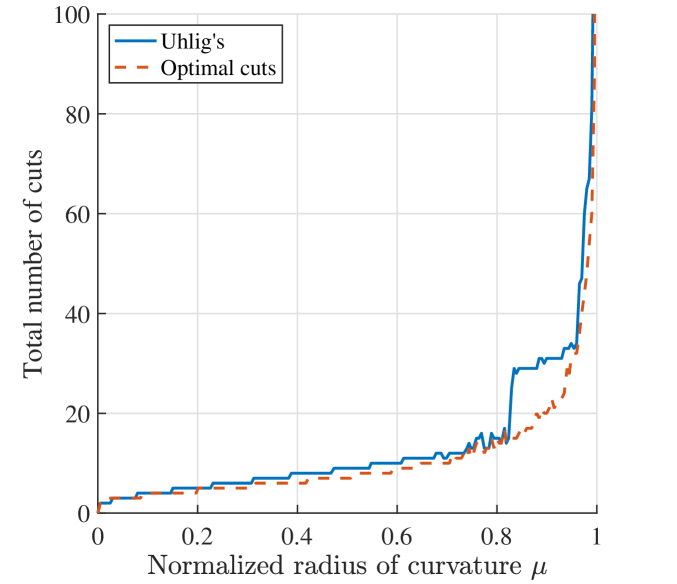
Figure 5: Using 200 different general matrices of the form $A+BXC$ with arbitrarily shaped fields of values and $\mu$ values roughly equally spaced between $0$ and $1$ at the outermost points in $W(A+BXC)$, Uhlig’s cutting procedure and optimal cuts are compared. For each example with a different value of $\mu$, we plot the total number of cuts needed to approximate the region of $\partial W(A+BXC)$ specified by supporting hyperplanes $L_{\theta_{\star}}$ and $L_{\theta_{j}}$ and the corner $c_{j}$ of $\mathcal{G}_{j}$ that they define, where $L_{\theta_{\star}}$ passes through the outermost point $b_{\star}$ and $\theta_{j}=\theta_{\star}-\tfrac{\pi}{50}$. The strong agreement of this plot with that of Fig. 4b empirically validates the generality of our convergence rate analyses, as Fig. 4b gives the analogous experiments for approximating the “same-sized” region of $\partial W(M)$ (in the sense that $\theta_{\star}-\theta_{j}=\tfrac{\pi}{50}$) for the parametric matrix $M$ given by Example 4.6 with $\mu\in(0,1]$.

For comparing our improved level-set and cutting-plane methods, we also set Algorithm 5.1 to do optimization via Newton’s method, and per Remark 2.5, had it add supporting hyperplanes for both $\lambda_{\mathrm{max}}$ and $\lambda_{\mathrm{min}}$ on every cut. For test problems, we used the Gear, Grcar, and FM examples used by Uhlig in [Uhl09], randn-based complex matrices, and $\mathrm{e}^{\mathbf{i}0.25\pi}((1-\mu)I+\mu K_{n})$ with $\mu=0.9999$ and $K_{n}$ from (4.1), which is a rotated version of Example 4.6 that we call Nearly Disk. In Table 4, we again see that Algorithm 3.1 is well optimized in terms of its overall possible efficiency, as it often only required a single computation with $R_{\gamma}-\lambda S$ and at most two. As predicted by our analysis, we also see that the cost of Algorithm 5.1 is highly correlated with the value of $\mu$. On Gear ($\mu\approx 0$), Algorithm 5.1 was extremely fast, essentially showing Q-superlinear convergence. In fact, on the Gear, Grcar, FM, and randn matrices, Algorithm 5.1 was much faster (3.4 to 234.2 times) than Algorithm 3.1 as $\mu<0.9$ for all of these problems. In contrast, for Nearly Disk ($\mu=0.9999$), Algorithm 5.1 was noticeably slower, with our level-set approach now being 5.7 to 11.5 times faster.

Table 4: The respective costs of Algorithms 3.1 and 5.1 are shown. The values of $\mu$ at outermost points are also shown, computed via Theorem 2.3.

			# of calls to eig($\cdot$)			Time (sec.)
			Alg. 3.1		Alg. 5.1	Alg. 3.1	Alg. 5.1
Problem	$n$	$\mu$	$R_{\gamma}-\lambda S$	$H(\theta)$	$H(\theta)$
Gear	320	$1.194\times 10^{-6}$	1	$2$	4	$1.2$	$0.1$
Gear	640	$1.499\times 10^{-7}$	1	$5$	3	$15.2$	$0.1$
Gear	1280	$1.878\times 10^{-8}$	1	$5$	3	$224.6$	$1.0$
Grcar	320	$0.6543$	1	$32$	28	$1.5$	$0.3$
Grcar	640	$0.6544$	1	$29$	29	$15.3$	$1.7$
Grcar	1280	$0.6544$	1	$27$	29	$215.0$	$12.8$
FM	320	$0.1851$	1	$11$	19	$1.3$	$0.1$
FM	640	$0.1836$	1	$8$	18	$10.9$	$0.5$
FM	1280	$0.1829$	1	$9$	18	$87.7$	$3.3$
randn	320	$0.7576$	1	$15$	40	$1.6$	$0.5$
randn	640	$0.8663$	2	$17$	67	$24.7$	$3.7$
randn	1280	$0.7971$	2	$23$	50	$203.5$	$22.0$
Nearly Disk	320	$0.9999$	1	$6$	1570	$1.7$	$20.0$
Nearly Disk	640	$0.9999$	1	$6$	1561	$13.2$	$88.6$
Nearly Disk	1280	$0.9999$	1	$7$	1556	$114.4$	$647.2$

Finally, we benchmark our hybrid algorithm and begin by comparing it with Algorithms 3.1 and 5.1. We tested our three algorithms on $n=400$ and $n=800$ examples with values $\mu\in\{0.1,0.2,\ldots,0.9,0.99,\ldots,0.9999999\}$ in order to represent the range of normalized radius of curvatures that may be encountered when minimizing the numerical radius. Since minimizing $r(A+BXC)$ to generate such matrices would be prohibitively expensive for these values of $n$ and $\mu$, we instead generated examples of the form $T_{n,\mu}=\mathrm{e}^{\mathbf{i}\theta}\begin{bmatrix}M&0\\ 0&D\end{bmatrix}$, where $\theta\in[0,2\pi)$ was chosen randomly, $M$ is an instance of Example 4.6 with the desired value of $\mu$ and dimension $n-100$, and $D\in\mathbb{C}^{100\times 100}$ is a complex diagonal matrix. In order to make $h(\theta)$ have many local maximizers, we chose $M$ such that $r(M)=1$ and then picked the elements of $D$ so that they were roughly placed near a circle drawn between $\partial W(\mathrm{e}^{\mathbf{i}\theta}M)$ and the unit circle, biased towards the latter; see Fig. 6a for a visualization. Fig. 6b shows how this choice of $D$ indeed causes $h(\theta)$ to have many local maximizers, while the randomly chosen $\mathrm{e}^{\mathbf{i}\theta}$ scalar means that the unique global maximizer may occur anywhere. The running times of our three algorithms on these $T_{n,\mu}$ examples are shown in Fig. 7. Once again, we see that the running time of Algorithm 3.1 remains fairly constant across all the values of $\mu$, while the running time of Algorithm 5.1 is much faster for small values of $\mu$ but then blows up as $\mu\to 1$. Most importantly, Fig. 7 verifies that our hybrid algorithm indeed remains efficient for all values of $\mu$ since it automatically detects when to switch from the cutting-plane approach to the level-set approach. In fact, our hybrid algorithm even becomes more efficient than Algorithm 3.1 for $\mu$ close to one. This is because when it switches to the level-set approach, Algorithm 5.1 often provided such good starting points that only one eigenvalue computation with $R_{\gamma}-\lambda S$ was needed. In contrast, Algorithm 3.1 always required two eigenvalue computations with $R_{\gamma}-\lambda S$ on our $T_{n,\mu}$ test problems.

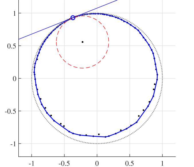
(a) $n=400$, $\mu=0.4$.

(b) $n=400$, $\mu=0.99$

Figure 6: Left: the field of values, eigenvalues, and the osculating circle at the unique point attaining the numerical radius are shown for one instance of $T_{n,\mu}$; to read the plot, see the caption of Fig. 1. Right: a plot of $h(\theta)$ for another instance of $T_{n,\mu}$.

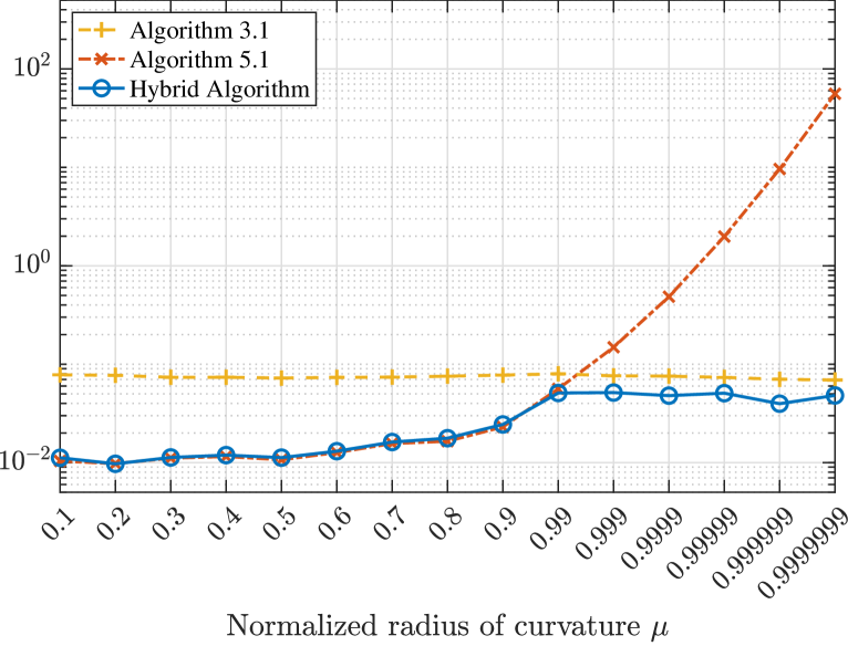
(a) $n=400$.

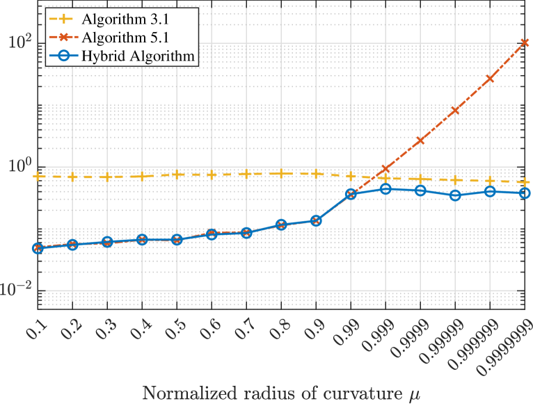
(b) $n=800$

Figure 7: Running times (in minutes, $\log_{10}$ scale) of the algorithms on $T_{n,\mu}$ with different normalized curvatures.

For our last set of experiments, we compare our hybrid algorithm with Mengi’s numr code and Uhlig’s NumRadius routine, which respectively implement the older methods described in [MO05] and [Uhl09]. As our hybrid algorithm allows up to $10000$ cutting-plane iterations by default, we also set the maximum allowed number of iterations of NumRadius to $10000$ (its default is only $200$). Furthermore, we set NumRadius to use eig, since we have standardized on using eig for all experiments. We tested the three codes on 39 matrices, all $800\times 800$ in size, with 20 taken from EigTool [Wri02], and another 19 taken from gallery in MATLAB; the matrices have a variety of different $\mu$ values at outermost points in the field of values, ranging from $\mu$ close to $0$ to $\mu=1$. Table 5 reports the performance data of the three codes on these problems, and from the table, it is immediately apparent that our hybrid algorithm remains efficient across all problems, while numr is quite slow on most of the problems, and NumRadius becomes more and more inefficient as $\mu\to 1$, as expected. Often our hybrid method is also the fastest method on each problem, and even when it is not, its performance is generally quite close to the fastest code, precisely because our algorithm automatically adapts to each problem. For problems with $\mu<0.831$, our hybrid is generally neck and neck with NumRadius, while being significantly faster than numr. Meanwhile, for problems with $\mu\geq 0.831$, i.e., problems for which optimal cuts and our hybrid algorithm have the most benefit, our hybrid algorithm is generally notably faster than NumRadius, and becomes dramatically faster for the three problems with $\mu=1.000$. Our hybrid algorithm is also much faster than numr on these $\mu\geq 0.831$ problems, except for the three $\mu=1.000$ examples, where numr ranged from 1.1–1.9 times faster. In some cases, we see that our method reduces the total number of eigenvalues computations with $H(\theta)$ (with respect to the total done by NumRadius) more than what is suggested by comparing the respective running times, e.g., on ’randcolu’; we believe this is because our MATLAB implementation is significantly more complex than NumRadius and so has a higher overhead. Overall, we see that the experiments in Table 5 paint a similar picture to our earlier experiments shown in Fig. 7. Using a compiled language and parallelism may help alleviate these remaining issues. Finally, we briefly discuss the accuracy of the computed estimates. On most of the problems, all three codes produced estimates with at least 14 digits of agreement. However, for the three $\mu=1.000$ examples, NumRadius reached the maximum of $10000$ iterations, and so its upper bound could only certify that seven or eight digits were correct. Meanwhile, when numr only performed one level-set test before terminating, we noticed that it returned estimates that were slightly too high, with errors in the tenth most significant digit; this appears to be a minor bug in the numr routine.

Table 5: The performance data of Mengi’s numr (MO), Uhlig’s NumRadius (U), and our hybrid algorithm (Hy.) are shown for various $800\times 800$ matrices from EigTool and gallery in MATLAB (matrices from gallery are shown in single-quotes in table). The problems are sorted in order of increasing $\mu$ value (all $\mu$ values are positive and shown to the first three decimal places), and the table is divided at $\mu\approx 0.831$, above which optimal cuts and our hybrid algorithm have the most benefits. The fastest running time per problem is typeset in bold.

		# of calls to eig($\cdot$)
		$R_{\gamma}-S$		$H(\theta)$			Time (sec.)
Problem	$\mu$	MO	Hy.	MO	U	Hy.	MO	U	Hy.
gausseidel(C)	0.000	1	0	1	3	3	23.1	0.4	0.4
’chebvand’	0.000	6	0	97	20	15	82.8	1.8	1.5
’dorr’	0.000	1	0	9	4	4	19.3	0.3	0.4
twisted	0.002	3	0	692	12	7	102.3	1.2	0.8
basor	0.007	3	0	14	9	12	57.6	1.0	1.3
convdiff	0.022	2	0	3256	6	5	224.2	0.5	0.5
davies	0.022	1	0	1617	9	11	112.5	0.9	1.1
airy	0.022	2	0	3209	8	11	224.9	0.8	1.1
landau	0.047	3	0	14	30	31	46.4	2.7	2.9
hatano	0.085	1	0	1	7	7	15.4	0.6	0.7
’clement’	0.131	1	0	9	26	13	19.0	2.4	1.4
’redheff’	0.155	1	0	5	8	8	14.2	0.7	0.8
’riemann’	0.284	1	0	5	10	9	17.9	1.0	0.9
’lesp’	0.330	2	0	1608	11	11	140.0	1.0	1.1
gausseidel(D)	0.392	1	0	1	12	10	15.6	1.2	1.0
’jordbloc’	0.500	1	0	1	13	12	21.3	1.2	1.2
transient	0.615	2	0	1117	28	28	114.3	2.7	2.7
frank	0.641	1	0	5	16	14	12.4	1.6	1.4
grcar	0.654	7	0	333	34	28	159.5	3.4	2.9
’dramadah’	0.659	1	0	5	16	14	13.9	1.5	1.5
’chow’	0.664	1	0	5	16	15	13.9	1.5	1.6
’triw’	0.669	2	0	1606	17	16	128.8	1.6	1.6
chebspec	0.727	1	0	5	18	17	13.1	1.7	1.7
kahan	0.741	2	0	11	18	18	28.9	1.7	1.9
’cycol’	0.807	7	0	69	54	59	88.6	5.0	6.0
gausseidel(U)	0.818	1	0	1	22	21	23.0	5.9	5.8
riffle	0.831	1	0	1	36	22	13.9	3.7	2.2
’randcolu’	0.837	5	0	63	62	53	78.2	5.8	5.6
random	0.843	5	0	45	72	56	77.9	7.1	6.0
’lotkin’	0.887	1	0	1	41	28	11.8	4.0	2.8
’randjorth’	0.924	5	0	55	82	62	64.4	8.0	6.5
’leslie’	0.929	1	0	1	43	33	13.5	4.2	3.5
’randsvd’	0.934	2	0	11	49	45	26.3	4.6	4.4
orrsommerfeld	0.935	3	0	4024	85	77	297.2	8.2	7.5
randomtri	0.944	6	0	54	97	75	84.3	10.0	7.8
demmel	0.998	2	0	11	258	233	25.9	24.9	24.2
’forsythe’	1.000	1	1	1	10000	35	13.6	957.2	26.1
’smoke’	1.000	1	1	1	10000	20	18.9	960.1	21.1
’parter’	1.000	1	1	1	10000	61	20.8	971.7	26.8
Total Time:							2479.8	3013.8	188.8

8 Conclusion

Via our new understanding of the local convergence rate of Uhlig’s cutting procedure, as well as how the overall cost of his method blows up for disk matrices, we have precisely explained why Uhlig’s method is sometimes much faster or much slower than the level-set method of Mengi and Overton. Moreover, this analysis has motivated our new hybrid algorithm that automatically switches between cutting-plane and level-set techniques in order to remain efficient across all numerical radius problems. Along the way, we have also identified inefficiencies in the earlier level-set and cutting-plane algorithms and addressed them via our improved versions of these two methodologies.

References

- [BB90] S. Boyd and V. Balakrishnan. A regularity result for the singular values of a transfer matrix and a quadratically convergent algorithm for computing its -norm. Systems Control Lett., 15(1):1–7, 1990.
- [BBMX02] P. Benner, R. Byers, V. Mehrmann, and H. Xu. Numerical computation of deflating subspaces of skew-Hamiltonian/Hamiltonian pencils. SIAM J. Matrix Anal. Appl., 24(1):165–190, 2002.
- [Ben02] I. Bendixson. Sur les racines d’une équation fondamentale. Acta Math., 25(1):359–365, 1902.
- [Ber65] C. A. Berger. A strange dilation theorem. Notices Amer. Math. Soc., 12:590, 1965.
- [BLO03] J. V. Burke, A. S. Lewis, and M. L. Overton. Robust stability and a criss-cross algorithm for pseudospectra. IMA J. Numer. Anal., 23(3):359–375, 2003.
- [BM18] P. Benner and T. Mitchell. Faster and more accurate computation of the norm via optimization. SIAM J. Sci. Comput., 40(5):A3609–A3635, October 2018.
- [BM19] P. Benner and T. Mitchell. Extended and improved criss-cross algorithms for computing the spectral value set abscissa and radius. SIAM J. Matrix Anal. Appl., 40(4):1325–1352, 2019.
- [BMO18] P. Benner, T. Mitchell, and M. L. Overton. Low-order control design using a reduced-order model with a stability constraint on the full-order model. In 2018 IEEE Conference on Decision and Control (CDC), pages 3000–3005, December 2018.
- [BS90] N. A. Bruinsma and M. Steinbuch. A fast algorithm to compute the -norm of a transfer function matrix. Systems Control Lett., 14(4):287–293, 1990.
- [BSV16] P. Benner, V. Sima, and M. Voigt. Algorithm 961: Fortran 77 subroutines for the solution of skew-Hamiltonian/Hamiltonian eigenproblems. ACM Trans. Math. Software, 42(3):Art. 24, 26, 2016.
- [Bye88] R. Byers. A bisection method for measuring the distance of a stable matrix to unstable matrices. SIAM J. Sci. Statist. Comput., 9:875–881, 1988.
- [DHT14] T. A Driscoll, N. Hale, and L. N. Trefethen. Chebfun Guide. Pafnuty Publications, Oxford, UK, 2014.
- [Fie81] M. Fiedler. Geometry of the numerical range of matrices. Linear Algebra Appl., 37:81–96, 1981.
- [GO18] A. Greenbaum and M. L. Overton. Numerical investigation of Crouzeix’s conjecture. Linear Algebra Appl., 542:225–245, 2018.
- [Gür12] M. Gürbüzbalaban. Theory and methods for problems arising in robust stability, optimization and quantization. PhD thesis, New York University, New York, NY 10003, USA, May 2012.
- [HJ91] R. A. Horn and C. R. Johnson. Topics in Matrix Analysis. Cambridge University Press, Cambridge, 1991.
- [HW97] C. He and G. A. Watson. An algorithm for computing the numerical radius. IMA J. Numer. Anal., 17(3):329–342, June 1997.
- [Joh78] C. R. Johnson. Numerical determination of the field of values of a general complex matrix. SIAM J. Numer. Anal., 15(3):595–602, 1978.
- [Kat82] T. Kato. A Short Introduction to Perturbation Theory for Linear Operators. Springer-Verlag, New York - Berlin, 1982.
- [Kip51] R. Kippenhahn. Über den Wertevorrat einer Matrix. Math. Nachr., 6(3-4):193–228, 1951.
- [KLV18] D. Kressner, D. Lu, and B. Vandereycken. Subspace acceleration for the Crawford number and related eigenvalue optimization problems. SIAM J. Matrix Anal. Appl., 39(2):961–982, 2018.
- [Kre62] H.-O. Kreiss. Über die Stabilitätsdefinition für Differenzengleichungen die partielle Differentialgleichungen approximieren. BIT, 2(3):153–181, 1962.
- [Küh15] W. Kühnel. Differential Geometry: Curves—Surfaces—Manifolds, volume 77 of Student Mathematical Library. American Mathematical Society, Providence, RI, third edition, 2015. Translated from the 2013 German edition by Bruce Hunt, with corrections and additions.
- [Lan64] P. Lancaster. On eigenvalues of matrices dependent on a parameter. Numer. Math., 6:377–387, 1964.
- [LO20] A. S. Lewis and M. L. Overton. Partial smoothness of the numerical radius at matrices whose fields of values are disks. SIAM J. Matrix Anal. Appl., 41(3):1004–1032, 2020.
- [Mat93] R. Mathias. Matrix completions, norms and Hadamard products. Proc. Amer. Math. Soc., 117(4):905–918, 1993.
- [Mit] T. Mitchell. ROSTAPACK: RObust STAbility PACKage. http://timmitchell.com/software/ROSTAPACK.
- [Mit20] T. Mitchell. Computing the Kreiss constant of a matrix. SIAM J. Matrix Anal. Appl., 41(4):1944–1975, 2020.
- [Mit21] T. Mitchell. Fast interpolation-based globality certificates for computing Kreiss constants and the distance to uncontrollability. SIAM J. Matrix Anal. Appl., 42(2):578–607, 2021.
- [MO05] E. Mengi and M. L. Overton. Algorithms for the computation of the pseudospectral radius and the numerical radius of a matrix. IMA J. Numer. Anal., 25(4):648–669, 2005.
- [MO22] T. Mitchell and M. L. Overton. On properties of univariate max functions at local maximizers. Optim. Lett., 2022. https://doi.org/10.1007/s11590-022-01872-y.
- [NW99] J. Nocedal and S. J. Wright. Numerical Optimization. Springer, New York, 1999.
- [Pea66] C. Pearcy. An elementary proof of the power inequality for the numerical radius. Michigan Math. J., 13:289–291, 1966.
- [TE05] L. N. Trefethen and M. Embree. Spectra and Pseudospectra: The Behavior of Nonnormal Matrices and Operators. Princeton University Press, Princeton, 2005.
- [TY99] B.-S. Tam and S. Yang. On matrices whose numerical ranges have circular or weak circular symmetry. Linear Algebra Appl., 302–303:193–221, 1999. Special issue dedicated to Hans Schneider (Madison, WI, 1998).
- [Uhl09] F. Uhlig. Geometric computation of the numerical radius of a matrix. Numer. Algorithms, 52(3):335–353, 2009.
- [Wat96] G. A. Watson. Computing the numerical radius. Linear Algebra Appl., 234:163–172, 1996.
- [Wri02] T. G. Wright. EigTool. http://www.comlab.ox.ac.uk/pseudospectra/eigtool/, 2002.