Data Augmentation for Histopathological Images Based on Gaussian-Laplacian Pyramid Blending

Abstract

Data imbalance is a major problem that affects several machine learning (ML) algorithms. Such a problem is troublesome because most of the ML algorithms attempt to optimize a loss function that does not take into account the data imbalance. Accordingly, the ML algorithm simply generates a trivial model that is biased toward predicting the most frequent class in the training data. In the case of histopathologic images (HIs), both low-level and high-level data augmentation (DA) techniques still present performance issues when applied in the presence of inter-patient variability; whence the model tends to learn color representations, which is related to the staining process. In this paper, we propose a novel approach capable of not only augmenting HI dataset but also distributing the inter-patient variability by means of image blending using the Gaussian-Laplacian pyramid. The proposed approach consists of finding the Gaussian pyramids of two images of different patients and finding the Laplacian pyramids thereof. Afterwards, the left-half side and the right-half side of different HIs are joined in each level of the Laplacian pyramid, and from the joint pyramids, the original image is reconstructed. This composition combines the stain variation of two patients, avoiding that color differences mislead the learning process. Experimental results on the BreakHis dataset have shown promising gains vis-à-vis the majority of DA techniques presented in the literature.

I Introduction

Cancer is a global health problem and can be the greatest barrier to the long life expectancy worldwide in the 21st century [1]. Breast cancer is the most prevalent cancer type among women in 140 out of 184 countries [2]. Its detection usually starts with self-examination and periodic mammography. These exams can identify lumps that will be examined in detail by ultrasound, computed tomography, or magnetic resonance imaging. When some characteristics that can point to a malignant tumor are detected by imaging exams, the final step is the biopsy, which is considered the gold-standard in the diagnosis process because it provides the most accurate diagnosis of the tumor type. The diagnosis procedure should be fast because some malignant tumors grow very fast and have high metastasis probability. Biopsies are a complex diagnosis tool, requiring the acquisition of material (e.g. fine-needle aspiration or open surgical biopsy), tissue treatment (slicing, staining and slide preparation) and analysis by an experienced pathologist. Such an analysis besides being time-consuming, it is subject to inter and intra-observer issues [3]. The variance in the results can be due to the pathologist experience or the hematoxylin and eosin (H&E) staining color differences, which may be related to stain manufacturers, storage age, and temperature.

Computer-aided diagnosis (CAD) systems can help in such an analysis by adding an extra opinion to the pathologist decision. CAD systems can rely on histopathologic images (HIs), which are obtained from tissue slides scanning, to make decisions about tumor characteristics, e.g. benign or malignant [4]. The automatic classification of HIs is a challenging problem in machine learning (ML) because HIs do not have the same structural aspect of macroscopic images such as people’s faces, cars, animals, or traffic signs. One structure that is important in HIs is the nucleus. In images stained with H&E, hematoxylin highlights the nuclei with a blueish color, and eosin highlights the cytoplasm and extracellular matrix in pink. The importance of the nucleus in tumor diagnosis is related to its quantity and format. When a region presents a highly abnormal amount of nuclei, this can be an indication of excessive cell multiplication, meaning a strong sign of a tumor. The format of the nuclei may also represent a signal of a tumor, this is called nucleus pleomorphism. Although blue and pink are the colors expected in H&E stained slides, it is common to face differences in intensity, saturation, and hue in the HIs. When analyzing an HI dataset, it is possible to note the differences in the slides from different patients, when they have been produced using different stain brands or faced variations during the whole process. The pathologist can understand this variation easily due to its expertise in looking at important HI features. However, color variations between patients may introduce a bias to ML algorithms. The image color of a patient’s slide does not vary if the staining process is the same, but the inter-patient slide color, even for the same tumor type, may be different. It is also possible to have images of different patients with similar colors, even if the tumor types are different. Therefore, color normalization may help minimize the color bias. However, color normalization algorithms require a target image as a reference to guide the normalization process [5, 6], which is a complex task that may cause loss of important characteristics. Furthermore, the classification result is closely related to such a reference image.

Another aspect related to the classification of HIs is the number of images available to train an ML model, especially deep learning (DL) models. DL models have been achieving impressive performance in several image classification tasks. However, as DL models usually have millions of parameters to tune, they require very large datasets for training to avoid overfitting the models. HI datasets, on the other hand, are usually small because analyzing and labeling HIs is expensive and requires experienced pathologists. Data augmentation (DA) has been actively used to circumvent this issue. Besides, HI datasets can also suffer from the data imbalance due to tumor occurrence rate and the biopsy priorities. As the biopsy procedure is expensive and time-consuming, it is usually carried out when malignant tumors are previously diagnosed through non-invasive exams.Furthermore, the biopsy is not required when most of the benign tumor types are detected. Therefore, it is common in the case of breast cancer biopsies to have a higher number of malignant HIs than benign HIs. Such a data imbalance also impacts on ML algorithms.

In this paper, we propose a novel approach for augmenting HI datasets, which distributes the inter-patient variability by means of image blending using the Gaussian-Laplacian pyramid. The main contributions of this paper are: (i) a novel data augmentation method that simultaneously provides color normalization and augmentation; (ii) a method to improve data classification by reducing the data imbalance; (iii) the advantages of using a texture convolutional neural network for HI classification. This paper is organized as follows: Section II presents related works found in the literature to data augmentation and data balancing, as well as their advantages and limitations. Section III briefly describes Gaussian-Laplacian pyramids, pyramid blending, and presents the proposed approach for data augmentation. Section IV describes the experimental setup used in this work. Results and conclusions are reported in Sections V and VI, respectively.

II Related Works

One way to circumvent the overfitting problem due to the small and imbalanced datasets is through DA. DA strategies have been exploited in many articles related to HIs, usually applying low-level transformation such as flip and rotation [7, 8, 9, 10]. Rotation, which consists of a turn of an image makes a congruent image of the original but facing another direction. Flip, likewise, creates a congruent mirror image of the original one. In both cases, the number of images increases but the heterogeneity in terms of texture is preserved. In other words, low-level transformations solve overfitting solely in terms of the number of images, but not in terms of inter-patient variability. Patching is another DA strategy that has been used with HIs [11, 12, 13]. This DA strategy divides an HI into some patches (overlapped or not). Thus, from one sample n samples are generated. Notwithstanding the gain in terms of the amount of data, some patches may not contain meaningful information in light of their size, the magnification of the original HI as well as their location in the original HIs. In the same way, some works also used DA strategies based on color disturbance [14]. Color disturbance contributed not only to increase the number of images but also to eliminate the color bias.

In addition to such DA strategies, generative adversarial networks (GANs) have also been used to create artificial instances from a particular dataset in such a way that the generated images retain similar characteristics vis-à-vis the original ones [15]. Besides, GANs have capabilities to mimic data distributions as well as to synthesize input images at remarkable levels of realism, because they maximize the probability density over the data by exploiting density ratio estimation [16]. Furthermore, GANs can find out the high dimensional latent distribution of data, which is the reason for the significant performance gains in terms of visual feature extraction. GANs have been used in medical imaging not only for DA but also for de-noising, segmentation, and reconstruction [17]

Concerning the data imbalance, due to tumor occurrence rate and the biopsy priorities, several approaches have been proposed to remedy this problem such as cost functions, ensemble learning, as well as algorithm-level and data-level approaches [18]. Data-level approaches generate new samples to balance the dataset. In the literature, it is also found some key techniques that are used to balance data at feature-level, such as SMOTE [19], ADASYN [20], and ROSE [21]. These techniques introduce synthetic examples through the interpolation between various positive instances that lie together. In the case of HIs, this means that new samples will be the approximation of existing samples, not solving the inter-patient diversity nonetheless.

III Proposed Method

The proposed method aims to improve the generalization ability of ML algorithms dealing with HIs, by considering the inter-patient variability. We propose the use of a blending method to composite images of different patients with the same type of tumor (benign or malignant). The present approach generates a new training image made up of half images of different patients. This strategy aims to avoid that a model learns color representations of patients, which, in fact, are related but to the staining process. While the straightforward blending of two images may produce artifacts owing to the adjacent pixel intensity difference, to remove such artifacts Gaussian-Laplacian pyramid was used.

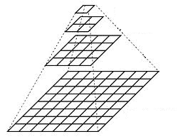
(a) Pyramid representation

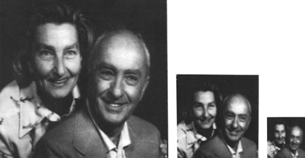
(b) Gaussian pyramid

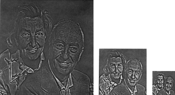
(c) Laplacian pyramid

Figure 1: An example of Gaussian and Laplacian pyramids from the same input image. (b) First three levels of Gaussian pyramid; (c) First three levels of Laplacian pyramid. Images adapted from [22].

III-A Gaussian-Laplacian Pyramid (GLP)

In signal processing and computer vision, pyramid representation (Fig. 1a) is the main type of multi-scale representation for computing image features on different scales. The pyramid is obtained by repeated smoothing and subsampling of an image or a signal. This concept is frequently used because it expresses computational efficiency approximation compared to other representations such as scale-space representation and multi-resolution analysis [23, 24, 25]. For generating the pyramid representation, different smoothing kernels have been brought forward and the binomial one strikingly shows up as useful and theoretically well-founded [26].

Accordingly, for a bi-dimensional image, the normalized binomial filter may be applied (1/4, 1/2, 1/4) in most cases twice or even more along all spatial dimensions, afterward, the subsampling of the image by a factor of two, which leads to efficient and compact multi-level representation. There are two main types of pyramids, namely, low-pass and band-pass [27, 22]. In order to develop filter-based representations by decomposing images into information on multiple scales as well as to extract features/structures of interest from an image, Gaussian pyramid (GP), Laplacian pyramid (LP), and wavelet pyramid are examples of the most frequently used pyramids.

The GP consists of low-pass filtered, reduced density, where subsequent images of the preceding level of the pyramid are weighted down by means of Gaussian average (or Gaussian blur) and scaled down, as shown in Figs. 1a and 1b. The base level ($l=0$) is defined as the original image. Formally speaking, assuming that $I(x,y)$ is a two-dimensional image, the GP is recursively defined in (1).

$$G_{l}(x,y)=\begin{cases}I(x,y),&\text{for level }l=0\\ \\ \sum\limits_{m=-2}^{2}\sum\limits_{n=-2}^{2}w(m,n)G_{l-1}(2x+m,2y+n),&\text{otherwise.}\end{cases}$$ (1)

where $m$ and $n$ are pixel coordinates and $w(m,n)$ is a Gaussian kernel which adheres to the following properties: separable, symmetric and each node at level $l$ contributes the same total weight to nodes at level $l+1$. The pyramid name arose from the fact that the Gaussian kernel nearly approximates a Gaussian function. This pyramid holds local averages on different scales, which has been leveraged for target localization and texture analysis [28, 29, 30].

In order to seamlessly stitching together image $I_{A}$ and image $I_{B}$ into a composite image on a scale-dependent way such that to avoid boundary artifacts, the LP is used. LP uses GP to blend images by preserving the significant feature meanwhile, as shown in Fig. 1c. The process is performed by downsizing the images into different levels (sizes) with Gaussian. Afterward, the Gaussian is expanded into the lower level and subtracts from the image at that level to acquire the Laplacian image. In other words, a level in LP is formed by the difference between that level in GP and expanded version of its upper level in GP. The smallest level, however, is not a different image for enabling the high-resolution image reconstruction. Formally speaking, assuming the GP $[{G}_{0},{G}_{1},\dots,{G}_{k}]$, where $k$ denotes the number of levels, the LP is obtained by computing:

$$L_{l}(x,y)=G_{l}(x,y)-4\sum\limits_{m=-2}^{2}\sum\limits_{n=-2}^{2}w(m,n)G_{l+1}\left(\frac{x-m}{2},\frac{y-n}{2}\right)$$ (2)

where $L_{l}(x,y)$ is the difference between $G_{l}(x,y)$ and an upsampled, smoothed version of $G_{l+1}(x,y)$. In the literature, LP is used for image compression, image enhancement, image analysis, and graphics [22].

III-B Pyramid Blending (PB)

Blending is a common task in several scientific applications whose purpose is to join smoothly two images or objects into a larger composite image in such a way that their respective boundaries junctions are unnoticed [22]. Fig. 2 shows an example of blending images $I_{A}$ and $I_{B}$ into composite images $I_{C,1}$ and $I_{C,2}$.

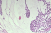
(a) $I_{A}$

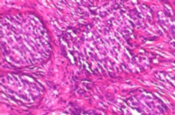
(b) $I_{B}$

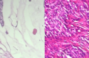
(c) $I_{C,1}$

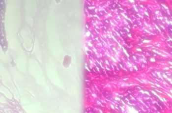
(d) $I_{C,2}$

Figure 2: Examples of image blending: (a) $I_{A}$ and (b) $I_{B}$ are two different images to be blended; (c) $I_{C,1}$ is a direct blending of $I_{A}$ and $I_{B}$; (d) $I_{C,2}$ is a multi-resolution blending of $I_{A}$ and $I_{B}$.

Let $I_{A}$ and $I_{B}$ be two images of the same resolution, and $I_{C}$ be the composite image from blending $I_{A,\text{left}}$ and $I_{B,\text{right}}$ which are the half-left side and the half-right side of $I_{A}$ and $I_{B}$, respectively. The direct blending is given by (3).

$$I_{C}=I_{A,\text{left}}+I_{B,\text{right}}$$ (3)

As shown in Fig. 2c, $I_{C,1}$ is often a composite in which the boundary junction is apparent when splining two images. The transition from one image to the other in case of direct blending may carry mismatch of both low and high frequencies.

III-C Proposed Approach for Data Augmentation

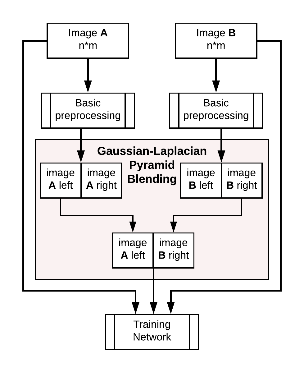
Figure 3: An overview of the proposed approach for DA based on GLPB.

This section presents an efficient approach using Gaussian-Laplacian pyramid blending (GLPB) for HI data augmentation. An overview of the proposed approach is shown in Fig. 3. The proposed approach for DA is based on blending two images of two different patients to generate the third image. As stated in Section III-B, the direct blending of $I_{A,\text{left}}$ and $I_{B,\text{right}}$ usually carries mismatch of low and high frequencies, therefore the boundary junction is evident and the resulting image does not look natural. Our hypothesis is that pyramid blending stands out as the most suitable solution to address this issue and produce natural-looking HIs. This process consists of decomposing each image into a set of spatial-frequency bands. Afterward, a band-pass composite can be constructed in each band by means of a transition zone. The latter is comparable in width to the wavelength representation in the band. To obtain the final composite, component band-pass composites are summed. The computational steps of the proposed multi-resolution splining procedure are quite feasible when pyramid methods are used [22].

In order to stitch together $I_{A,\text{left}}$ and $I_{B,\text{right}}$ into a composite image with minimum or no apparent junction boundaries, the Laplacian pyramid is used to smoothing the boundary on a scale-dependent way to avoid boundary artifacts. Assuming that $I_{A}$ and $I_{B}$ have the same resolution, the proposed approach is made up of the following steps:

1. Input: Patient images $I_{A}$ and $I_{B}$, and a (binary) mask $R$ that specifies the blend ($0=I_{A}$, $1=I_{B}$), with $A\neq B$.

2. Build $I_{A_{i}}$’s (AL) Laplacian pyramid, $i\in 0...N$; $I_{B_{j}}$’s (BL) Laplacian pyramid, $j\in 0...N$, and $R_{p}$’s (RG) Gaussian pyramid $p\in 0...N$;

3. Build a Laplacian pyramid for the result F, using linear interpolation over every pixel, with a blend mask given at different levels of detail, for every pyramid level k:
     $FL_{k}(r,c)=(1-RG_{k}(r,c))*AL_{k}(r,c)+RG_{k}(r,c)*BL_{k}(r,c)$, where r and c are row and column, respectively;

4. Reconstitute the full-resolution image for F, by building F Gaussian (FG) and F Laplacian (FL) as follow:
   $F=FG_{0}$ from $FL_{i},i\in 0...N$.
   $FG_{N}=FL_{N}$
   $FG_{k}=FL_{k}+EXPAND(FG_{k+1})$.

Fig. 4 illustrates the results achieved by the proposed method on HIs from the BreakHis dataset [31].

(a) Image blending with pyramids (left), examples of blending in which the stitching not evident (right).

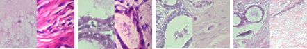
(b) Examples of blending results in which the stitching is evident.

Figure 4: Examples of HI blending: (a) Image C is the composite of the pyramid blending of Image A and Image B; images on the right side are composite images generated by pyramid blending of different patients. Each image is the result of different images of different magnitudes such as 40$\times$, 100$\times$, 200$\times$ and 400$\times$ as specified on the right side of each image; (b) samples in which the blending process generated artifacts.

IV Experimental Setup

The dataset used in the experiments is BreakHis [31]. It consists of 7,909 breast cancer histopathologic images. The images are labeled following eight types of tumor, four malignant and four benign. The distribution of images is imbalanced according to the tumor type, due to the prevalence of certain tumor types in the population, presented in Table I. The original image size is 700$\times$460 pixels and 8-bits RGB. We used images downsized by half to reduce the CNN overhead. The classification considered but benign and malignant classes, that is, all benign tumors are considered as a single class and all malignant tumors as another class.

TABLE I: Image and patient distribution in the BreakHis dataset.

Tissue		# of	# of
Type	Tumor Type	Images	Patients
Benign	Adenosis	444	4
	Fibroadenoma	1,014	10
	Phyllodes tumor	453	3
	Tubular adenoma	569	7
	Total	2,368	24
Malign	Ductal carcinoma	3,451	38
	Lobular carcinoma	626	5
	Mucinous carcinoma	792	9
	Papillary carcinoma	560	6
	Total	5,429	58

HIs do not have a defined geometric structure like macroscopic images do, thus, we use a compact CNN model, named Texture CNN (TCNN) [32]. The network architecture is presented in Table II and it consists of two convolutional layers interleaved with batch normalization layers, a global average pooling, and two fully connected layers. All layers except the last one use ReLU activation function. The implementation was done using Pytorch. We used adadelta for optimization with a learning rate of 0.1 and 25 epochs. The number of images used in the experiments is reduced, taking into account that the 7,909 images are divided into four magnification factors. This is the other reason for employing TCNN, which has fewer parameters compared to other CNN architectures such as VGG or ResNet.

TABLE II: The architecture of TCNN.

Layer	Size	Kernel	Filters
Input	350$\times$230	-	3
Conv2D	350$\times$230	3	32
BatchNorm	350$\times$230	-	-
ReLU	350$\times$230	-	-
Conv2D	350$\times$230	3	32
BatchNorm	350$\times$230	-	-
ReLU	350$\times$230	-	-
GlobalAveragePool	1$\times$1	-	32
FullyConnected	32	-	-
ReLU	32	-	-
FullyConnected	16	-	-
SoftMax	2	-	-

We analyzed the impact of DA on TCNN by varying the augmentation factor. It is worthy of note that the comparisons herein are more focused on the imbalance problem of the dataset, meaning that we used the GLPB only to generate new images of the benign type of tumor. We have not applied the GLPB in the malignant images. We generated as many benign images as necessary to equalize the amount of benign and malignant images. The GLPB approach was evaluated using no DA (GLPB), using additional color DA over the entire set of equalized images (benign and maligned) to double the size of the training set (GLPB2$\times$) and to augment it six times (GLPB6$\times$). Therefore, all experiments with GLPB were based in the GLPB equalized dataset.

Furthermore, we have also implemented a blending algorithm to minimize the boundary junction formed between the combination of the two images after a direct blending. This blending (Mix) applies a color linear combination in the middle of the composite images (half of each image), resulting in a smooth transition between them. We applied the Mix between benign random images (MixB&M) and we also mixed images of the same sub-type of the tumor, e.g. adenoma images of two different patients (MixSub). We also compared our results with the original dataset without DA and class balancing (NoAug). Furthermore, the classification results without balancing, but using only color DA are also presented (Aug2$\times$). An interesting analysis regarding DA and TCNN can be found in [33], which used an approach based on the color information [34]. In addition, we have also used an approach based on GANs to generate a combination of images between patients. We used the same CycleGAN proposed by [35], which generates new images combining features from two origins. We trained a single model of the CycleGAN using all images from the dataset, from both the classes. During the training process, we only used pairs of the same class as samples (A and B in the CycleGAN were of the same class), so the transforming process of the GAN was restricted inside classes. The images to the augmentation process were also generated inside a single class, not mixing images from benign or malignant classes. We combined the same images used in the GLPB approach with the intention of balancing the dataset and also applied 2$\times$ (GAN2$\times$) and 6$\times$ (GAN6$\times$) DA.

In total we have carried out 10 experiments, three involving the GLPB approach, three with the GAN balanced dataset, two with no balancing and two using the Mix approach. All experiments were repeated five times according to the experimental setup proposed by [31], which is a five-fold repeated holdout. The proportion of data for training and test is 70% and 30% patient-wise respectively, which means that no patient has parts of his/her images in training or test simultaneously. Another important aspect of the experiments is that we did not mix images of different magnifications. As a result of the experimental setup, we performed 200 executions.

V Results and Discussion

The experiment results are summarized in Table III. Our results are reported following image-level and patient-level. For image-level, we also present the balanced accuracy, which in this two-class problem is the mean of specificity and sensitivity. All results are the mean of the five folds followed by their standard deviation. Our approach performed better than other methods compared with 400$\times$ and 200$\times$ magnifications. We can also highlight the result for Aug2$\times$ and 200$\times$ magnifications where the patient’s accuracy is high, close to our method, but when looking at the balanced accuracy, it does not present good balanced image-level accuracy. In other words, it only performed well in one class, which shows the importance of presenting balanced accuracy due to the dataset imbalance. The approaches of mixing images, both by GLPB and Mix presented good results with a small advantage margin to GLPB.

TABLE III: Five-fold mean image-level accuracy, image-level balanced accuracy and patient-level accuracy for four magnification factors. The best values are higlighted in bold font.

		Magnification
Method		400$\times$	200$\times$	100$\times$	40$\times$
Image	GLPB	0.872 $\pm$ 0.045	0.884 $\pm$ 0.050	0.814 $\pm$ 0.048	0.821 $\pm$ 0.064
	GLPB2$\times$	0.851 $\pm$ 0.061	0.884 $\pm$ 0.058	0.830 $\pm$ 0.057	0.808 $\pm$ 0.071
	GLPB6$\times$	0.837 $\pm$ 0.037	0.876 $\pm$ 0.049	0.823 $\pm$ 0.046	0.787 $\pm$ 0.054
	MixB&M	0.871 $\pm$ 0.050	0.883 $\pm$ 0.050	0.824 $\pm$ 0.045	0.841 $\pm$ 0.055
	MixSub	0.821 $\pm$ 0.065	0.874 $\pm$ 0.059	0.822 $\pm$ 0.055	0.803 $\pm$ 0.065
	NoAug	0.692 $\pm$ 0.067	0.816 $\pm$ 0.063	0.698 $\pm$ 0.026	0.678 $\pm$ 0.034
	Aug2$\times$	0.798 $\pm$ 0.064	0.874 $\pm$ 0.040	0.771 $\pm$ 0.011	0.745 $\pm$ 0.063
	GAN	0.851 $\pm$ 0.050	0.870 $\pm$ 0.056	0.804 $\pm$ 0.042	0.774 $\pm$ 0.085
	GAN2$\times$	0.849 $\pm$ 0.057	0.874 $\pm$ 0.057	0.821 $\pm$ 0.032	0.805 $\pm$ 0.067
	GAN6$\times$	0.839 $\pm$ 0.041	0.877 $\pm$ 0.049	0.813 $\pm$ 0.021	0.795 $\pm$ 0.049
Balanced	GLPB	0.847 $\pm$ 0.043	0.875 $\pm$ 0.063	0.795 $\pm$ 0.044	0.803 $\pm$ 0.049
	GLPB2$\times$	0.845 $\pm$ 0.056	0.878 $\pm$ 0.068	0.821 $\pm$ 0.064	0.808 $\pm$ 0.069
	GLPB6$\times$	0.831 $\pm$ 0.033	0.868 $\pm$ 0.062	0.820 $\pm$ 0.047	0.795 $\pm$ 0.051
	MixB&M	0.846 $\pm$ 0.051	0.866 $\pm$ 0.065	0.793 $\pm$ 0.064	0.807 $\pm$ 0.065
	MixSub	0.818 $\pm$ 0.063	0.861 $\pm$ 0.069	0.793 $\pm$ 0.063	0.792 $\pm$ 0.074
	NoAug	0.547 $\pm$ 0.073	0.720 $\pm$ 0.073	0.543 $\pm$ 0.030	0.513 $\pm$ 0.026
	Aug2$\times$	0.711 $\pm$ 0.087	0.819 $\pm$ 0.053	0.661 $\pm$ 0.010	0.617 $\pm$ 0.095
	GAN	0.816 $\pm$ 0.057	0.847 $\pm$ 0.064	0.763 $\pm$ 0.043	0.709 $\pm$ 0.129
	GAN2$\times$	0.834 $\pm$ 0.052	0.853 $\pm$ 0.063	0.788 $\pm$ 0.038	0.769 $\pm$ 0.061
	GAN6$\times$	0.821 $\pm$ 0.033	0.855 $\pm$ 0.050	0.768 $\pm$ 0.026	0.761 $\pm$ 0.056
Patient	GLPB	0.882 $\pm$ 0.043	0.896 $\pm$ 0.054	0.835 $\pm$ 0.022	0.845 $\pm$ 0.042
	GLPB2$\times$	0.857 $\pm$ 0.061	0.891 $\pm$ 0.067	0.852 $\pm$ 0.047	0.825 $\pm$ 0.067
	GLPB6$\times$	0.847 $\pm$ 0.032	0.887 $\pm$ 0.055	0.841 $\pm$ 0.048	0.789 $\pm$ 0.063
	MixB&M	0.877 $\pm$ 0.053	0.890 $\pm$ 0.056	0.835 $\pm$ 0.029	0.860 $\pm$ 0.049
	MixSub	0.823 $\pm$ 0.053	0.885 $\pm$ 0.063	0.834 $\pm$ 0.044	0.826 $\pm$ 0.059
	NoAug	0.711 $\pm$ 0.054	0.830 $\pm$ 0.053	0.708 $\pm$ 0.025	0.689 $\pm$ 0.022
	Aug2$\times$	0.815 $\pm$ 0.066	0.891 $\pm$ 0.035	0.771 $\pm$ 0.021	0.755 $\pm$ 0.066
	GAN	0.856 $\pm$ 0.053	0.884 $\pm$ 0.056	0.813 $\pm$ 0.046	0.796 $\pm$ 0.073
	GAN2$\times$	0.857 $\pm$ 0.062	0.883 $\pm$ 0.062	0.842 $\pm$ 0.025	0.825 $\pm$ 0.057
	GAN6$\times$	0.850 $\pm$ 0.047	0.886 $\pm$ 0.055	0.835 $\pm$ 0.023	0.814 $\pm$ 0.043

Remarkably, 200$\times$ magnification is the most significant result for our proposal, presenting the best accuracy (image, image balanced, and patient accuracy). Table IV shows that the results achieved by the GLPB outperform some state-of-the-art results. We included in Table IV only results that followed the same fold distribution. Additional results on the BreakHis dataset using different fold distributions can be found in [36]. In Table IV, the Baseline method is based on handcrafted feature extractors for texture and obtained better results with 200$\times$ magnification. AlexNet and Deep Features methods are based on CNNs and present better results in 100$\times$ and 40$\times$ magnifications. Our approach used a compact CNN, designed for texture recognition, which also presented good results for 200$\times$ magnification.

We present in Fig. 5 an example of HIs of two tumor types with two different magnifications. Figs. 5a and 5b are Ductal Carcinoma images of 40$\times$ and 400$\times$ magnifications. Figs. 5a and 5b are Adenoma images of 40$\times$ and 400$\times$ magnification factors. These images highlight the differences in the objective into which the filters are trained. In the 40$\times$ magnification, it is difficult to identify nucleus pleomorphism since they are too small. On the other hand, this magnification makes easy to detect forms like the ones that characterize papillary carcinoma. The characteristics of magnifications impact in the network used, taking into account that the small network does not have the capabilities of large objects recognizing, only textures. To the same extent, future work studies may include shallow methods in order to compare the performance of GLPB vis-à-vis other techniques of undersampling and oversampling such as SMOTE and NearMiss algorithms.

TABLE IV: State-of-the-art patient accuracy results with the same fold split.

	Magnification
Method	400$\times$	200$\times$	100$\times$	40$\times$
Baseline [31]	0.823 $\pm$ 0.038	0.851 $\pm$ 0.031	0.821 $\pm$ 0.049	0.838 $\pm$ 0.041
AlexNet [12]	0.817 $\pm$ 0.049	0.853 $\pm$ 0.038	0.845 $\pm$ 0.024	0.886 $\pm$ 0.056
Deep Features [37]	0.861 $\pm$ 0.062	0.863 $\pm$ 0.035	0.884 $\pm$ 0.048	0.840 $\pm$ 0.069
Mi [38]	0.827 $\pm$ 0.030	0.872 $\pm$ 0.043	0.891 $\pm$ 0.052	0.921 $\pm$ 0.059
GLPB	0.882 $\pm$ 0.043	0.896 $\pm$ 0.054	0.835 $\pm$ 0.022	0.845 $\pm$ 0.042

(a) DC 40$\times$

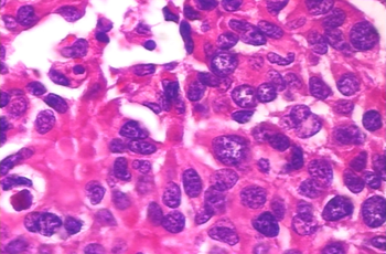
(b) DC 400$\times$

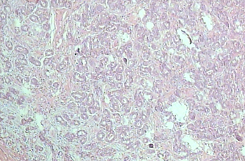
(c) A 40$\times$

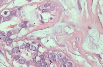
(d) A 400$\times$

Figure 5: Comparison of Ductal Carcinoma (DC) and Adenoma (A) images with magnifications of (a) 40$\times$ (b) 400$\times$ (c) 40$\times$ (d) 400$\times$

Finally, Table V presents the subclass classification result for 40$\times$ and 200$\times$ magnifications using GLPB2$\times$. These are the two scenarios where GLPB achieved the worst and the best performance, respectively. We consider 40$\times$ magnifications the worst result because the difference to the state-of-the-art is the highest one. We also show the Aug2$\times$ result for 200$\times$ magnification that achieved good patient accuracy results but presented poor balanced accuracy results. It can be seen in Table V, where the Malignant tumors were much better identified than the Benign.

TABLE V: Classification accuracy considering subclass distribution for 40$\times$ and 200$\times$ magnifications using GLPB2$\times$ and 200$\times$ magnification with Aug2$\times$. Adenoma (A), Fibroadenoma (F), Tubular Adenoma (TA), Phyllodes Tumor (PT), Ductal Carcinoma (DC), Papillary Carcinoma (PC), Mucinous Carcinoma (MC) and Lobular Carcinoma (LC)

		Predicted
		B	M	B	M	B	M	B	M	B	M
		Mag 40$\times$ GLPB2$\times$
Benign	A	0.71	0.29	0.68	0.32	1.00	0.00	1.00	0.00	0.88	0.13
	F	0.91	0.09	0.85	0.15	0.77	0.23	0.75	0.25	0.78	0.22
	TA	0.73	0.27	0.56	0.44	1.00	0.00	0.48	0.52	0.51	0.49
	PT	0.74	0.26	1.00	0.00	1.00	0.00	1.00	0.00	0.55	0.45
Malignant	DC	0.12	0.88	0.08	0.92	0.10	0.90	0.23	0.77	0.05	0.95
	PC	0.62	0.38	0.75	0.25	0.11	0.89	0.69	0.31	0.18	0.82
	MC	0.13	0.87	0.40	0.60	0.11	0.89	0.44	0.56	0.07	0.93
	LC	0.11	0.89	0.07	0.93	0.00	1.00	0.04	0.96	0.00	1.00
		Mag 200$\times$ GLPB2$\times$
Benign	A	0.81	0.19	0.56	0.44	0.98	0.02	0.98	0.02	0.96	0.04
	F	0.98	0.02	1.00	0.00	1.00	0.00	0.72	0.28	0.97	0.03
	TA	0.86	0.14	0.55	0.45	1.00	0.00	0.58	0.42	0.90	0.10
	PT	0.75	0.25	0.93	0.07	0.93	0.07	1.00	0.00	0.78	0.22
Malignant	DC	0.09	0.91	0.05	0.95	0.07	0.93	0.11	0.89	0.05	0.95
	PC	0.32	0.68	0.69	0.31	0.00	1.00	0.47	0.53	0.02	0.98
	MC	0.05	0.95	0.15	0.85	0.02	0.98	0.42	0.58	0.12	0.88
	LC	0.09	0.91	0.00	1.00	0.00	1.00	0.00	1.00	0.00	1.00
		Mag 200$\times$ Aug2$\times$
Benign	A	0.40	0.60	0.42	0.58	0.66	0.34	0.65	0.35	0.63	0.37
	F	0.82	0.18	1.00	0.00	0.98	0.02	0.71	0.29	0.66	0.34
	TA	0.49	0.51	0.55	0.45	0.90	0.10	0.51	0.49	0.46	0.54
	PT	0.54	0.46	0.79	0.21	0.71	0.29	0.76	0.24	0.54	0.46
Malignant	DC	0.01	0.99	0.02	0.98	0.01	0.99	0.01	0.99	0.00	1.00
	PC	0.11	0.89	0.54	0.46	0.00	1.00	0.06	0.94	0.00	1.00
	MC	0.00	1.00	0.04	0.96	0.00	1.00	0.04	0.96	0.01	0.99
	LC	0.01	0.99	0.00	1.00	0.00	1.00	0.00	1.00	0.00	1.00

VI Conclusion

This paper presented a novel method for data augmentation based on Gaussian and Laplacian pyramids. We investigated how the classifiers can be improved in terms of the generalization ability considering the inter-patient variability. We stated that a DA could be decomposed into image blending such that from two images the third can be generated, where each one is from a different patient while producing both a balanced dataset and good classification accuracy, precision, and recall.

It is essential to consider that Gaussian-Laplacian pyramids provide a powerful mathematical tool for representing multi-resolutions of an image as well as a blending between two images of the same class while finding the most favorable seam and avoiding artifacts along boundaries. Thence, in this paper, blending images helped to augment the dataset and to balance the respective classes under investigation, meanwhile performing at comparable accuracy as other state-of-the-art methods. The blending method can provide improvements on the results of the other state-of-the-art methods, considering that it works as a preprocessing stage and can be used together with other methods as well. Accordingly, the proposed method is promising to circumvent the limitation of data, in particular for deep methods where the classification considers HIs as whole images.

References

- [1] F. Bray, J. Ferlay, I. Soerjomataram, R. L. Siegel, L. A. Torre, and A. Jemal, “Global cancer statistics 2018: GLOBOCAN estimates of incidence and mortality worldwide for 36 cancers in 185 countries,” CA: A Cancer J Clinicians, vol. 68, no. 6, pp. 394–424, 2018.
- [2] L.A. Torre, F. Islami, R.L. Siegel, E.M. Ward, and A. Jemal, “Global cancer in women: Burden and trends,” Cancer Epid Prev Biom, vol. 26, no. 4, pp. 444–457, 2017.
- [3] J.-P. Belloq, E. Anger, J.-F. Flejou, P. Galateau, F. Gaulard, M. Guiu, J.-F. Michiels, J.-P. Saint-Andre, J.Y. Scoazec, M.-C. Vacher-Lavenu, P. Camparo, F. Capron, M.-P. Chenard, J. Chetritt, J.-P. Chigot, B. Cochand-Priollet, J.-M. Coindre, and M.-C. Copin, “Sécuriser le diagnostic en anatomie et cytologie pathologiques en 2011. l’erreur diagnostique: entre discours et réalité,” in Annales de pathologie, 2011.
- [4] J. de Matos, A.S.Britto Jr., L.E.S. Oliveira, and A.L. Koerich, “Histopathologic image processing: A review,” CoRR, vol. abs/1904.07900, 2019.
- [5] B. Ehteshami Bejnordi, G. Litjens, N. Timofeeva, I. Otte-Höller, A. Homeyer, N. Karssemeijer, and J. A. van der Laak, “Stain specific standardization of whole-slide histopathological images,” IEEE Trans Med Imag, vol. 35, no. 2, pp. 404–415, 2016.
- [6] F. Ciompi, O. Geessink, B.E. Bejnordi, G.S. de Souza, A. Baidoshvili, G. Litjens, B. van Ginneken, I. Nagtegaal, and J. van der Laak, “The importance of stain normalization in colorectal tissue classification with convolutional networks,” in IEEE 14th Intl Symp Biom Imag, 2017, pp. 160–163.
- [7] G. Zhang, M. Xiao, and Y.-H. Huang, “Histopathological image recognition with domain knowledge based deep features,” in Intelligent Computing Methodologies, D.-S. Huang, M.M. Gromiha, K. Han, and A. Hussain, Eds. 2018, pp. 349–359, Springer Intl Pub.
- [8] V. Gupta and A. Bhavsar, “Sequential modeling of deep features for breast cancer histopathological image classification,” in IEEE Conf Comp Vis Patt Recog Works, 2018.
- [9] Z. Gandomkar, P.C. Brennan, and C. Mello-Thoms, “Mudern: Multi-category classification of breast histopathological image using deep residual networks,” Artif Intell Med, vol. 88, pp. 14–24, 2018.
- [10] D. Bardou, K. Zhang, and S.M. Ahmad, “Classification of breast cancer based on histology images using convolutional neural networks,” IEEE Access, vol. 6, pp. 24680–24693, 2018.
- [11] K. Roy, D. Banik, D. Bhattacharjee, and M. Nasipuri, “Patch-based system for classification of breast histology images using deep learning,” Comput Med Imag Graph, vol. 71, pp. 90–103, 2019.
- [12] F. A. Spanhol, L. S. Oliveira, C. Petitjean, and L. Heutte, “Breast cancer histopathological image classification using convolutional neural networks,” in Intl J Conf Neural Networks, 2016, pp. 2560–2567.
- [13] J. de Matos, A.S. Britto Jr., L.E.S. Oliveira, and A.L. Koerich, “Double transfer learning for breast cancer histopathologic image classification,” in Intl J Conf Neural Networks, 2019, pp. 1–8.
- [14] H. Lin, H. Chen, Q. Dou, L. Wang, J. Qin, and P. Heng, “Scannet: A fast and dense scanning framework for metastastic breast cancer detection from whole-slide image,” in IEEE Winter Conf Appl Comp Vis, 2018, pp. 539–546.
- [15] I. Goodfellow, J. Pouget-Abadie, M. Mirza, B. Xu, D. Warde-Farley, S. Ozair, A. Courville, and Y. Bengio, “Generative adversarial nets,” in Adv Neural Inf Proc Sys, 2014, pp. 2672–2680.
- [16] P. Isola, J.-Y. Zhu, T. Zhou, and A.A. Efros, “Image-to-image translation with conditional adversarial networks,” in IEEE Conf Comp Vis Patt Recog, 2017, pp. 1125–1134.
- [17] S. Kazeminia, C. Baur, A. Kuijper, B. van Ginneken, N. Navab, S. Albarqouni, and A. Mukhopadhyay, “Gans for medical image analysis,” arXiv preprint arXiv:1809.06222, 2018.
- [18] A. Fernandez, S. Garca, M. Galar, R.C. Prati, B. Krawczyk, and F. Herrera, Learning from Imbalanced Data Sets, Springer, 1st edition, 2018.
- [19] N.V. Chawla, K.W. Bowyer, L.O. Hall, and W.P. Kegelmeyer, “Smote: synthetic minority over-sampling technique,” J Artif Intell Res, vol. 16, pp. 321–357, 2002.
- [20] H. He, Y. Bai, E.A. Garcia, and S. Li, “Adasyn: Adaptive synthetic sampling approach for imbalanced learning,” in IEEE Intl J Conf Neural Networks, 2008, pp. 1322–1328.
- [21] G. Menardi and N. Torelli, “Training and assessing classification rules with imbalanced data,” Data Min Knowl Discov, vol. 28, no. 1, pp. 92–122, 2014.
- [22] E.H. Adelson, C. H. Anderson, J.R. Bergen, P.J. Burt, and J.M. Ogden, “Pyramid methods in image processing,” RCA Engineer, vol. 29, no. 6, pp. 33–41, 1984.
- [23] J.L. Crowley and O. Riff, “Fast computation of scale normalised gaussian receptive fields,” in Intl Conf Scale-Space Theor Comp Vis, 2003, pp. 584–598.
- [24] D. G. Lowe, “Distinctive image features from scale-invariant keypoints,” Intl J Comp Vis, vol. 60, no. 2, pp. 91–110, 2004.
- [25] P.J. Burt, “Fast filter transform for image processing,” Comp Graph Image Proc, vol. 16, no. 1, pp. 20–51, 1981.
- [26] T. Lindeberg, Scale-space theory in computer vision, vol. 256, Springer Sci & Bus Media, 2013.
- [27] P. Burt and E. Adelson, “The laplacian pyramid as a compact image code,” IEEE Trans Comm, vol. 31, no. 4, pp. 532–540, 1983.
- [28] P.J. Burt, “Fast algorithms for estimating local image properties,” Comp Vis Graph Image Proc, vol. 21, no. 3, pp. 368–382, 1983.
- [29] L.I. Larkin and P.J. Burt, “Multi-resolution texture energy measures,” in IEEE Conf Comp Vis Patt Recog, 1983.
- [30] C.H. Anderson, P.J. Burt, and G.S. Van Der Wal, “Change detection and tracking using pyramid transform techniques,” in Intell Robots Comp Vis IV, 1985, vol. 579, pp. 72–78.
- [31] F. A. Spanhol, L. S. Oliveira, C. Petitjean, and L. Heutte, “A dataset for breast cancer histopathological image classification,” IEEE Trans Biom Eng, vol. 63, no. 7, pp. 1455–1462, 2016.
- [32] V. Andrearczyk and P.F. Whelan, “Using filter banks in convolutional neural networks for texture classification,” Patt Recog Lett, vol. 84, pp. 63–69, 2016.
- [33] J. de Matos, A. de Souza Britto, L. E. S. de Oliveira, and A. L. Koerich, “Texture cnn for histopathological image classification,” in IEEE 32nd Intl Symp Comp-Based Med Sys, 2019, pp. 580–583.
- [34] D. Tellez, M. Balkenhol, I. Otte-Höller, R. van de Loo, R. Vogels, P. Bult, C. Wauters, W. Vreuls, S. Mol, N. Karssemeijer, G. Litjens, J. van der Laak, and F. Ciompi, “Whole-slide mitosis detection in h e breast histology using phh3 as a reference to train distilled stain-invariant convolutional networks,” IEEE Trans Med Imag, vol. 37, no. 9, pp. 2126–2136, 2018.
- [35] J. Zhu, T. Park, P. Isola, and A.A. Efros, “Unpaired image-to-image translation using cycle-consistent adversarial networks,” in IEEE Intl Conf Comp Vis, 2017, pp. 2242–2251.
- [36] Y. Benhammou, B. Achchab, F. Herrera, and S. Tabik, “Breakhis based breast cancer automatic diagnosis using deep learning: Taxonomy, survey and insights,” Neurocomputing, vol. 375, pp. 9–24, 2020.
- [37] F.A. Spanhol, L.S. Oliveira, P.R. Cavalin, C. Petitjean, and L. Heutte, “Deep features for breast cancer histopathological image classification,” in IEEE Intl Conf Sys Man Cybern, 2017, pp. 1868–1873.
- [38] P.J. Sudharshan, C. Petitjean, F. Spanhol, L.E. Oliveira, L. Heutte, and P. Honeine, “Multiple instance learning for histopathological breast cancer image classification,” Expert Sys Appl, vol. 117, pp. 103–111, 2019.