The ELM Survey. VIII. 98 Double White Dwarf Binaries

Abstract

We present the final sample of 98 detached double white dwarf (WD) binaries found in the Extremely Low Mass (ELM) Survey, a spectroscopic survey targeting $<$0.3 $M_{\odot}$ He-core WDs completed in the Sloan Digital Sky Survey footprint. Over the course of the survey we observed ancillary low mass WD candidates like GD 278, which we show is a $P=0.19$ d double WD binary, as well as candidates that turn out to be field blue straggler/subdwarf A-type stars with luminosities too large to be WDs given their Gaia parallaxes. Here, we define a clean sample of ELM WDs that is complete within our target selection and magnitude range $15<g_{0}<20$ mag. The measurements are consistent with 100% of ELM WDs being $0.0089<P<1.5$ d double WD binaries, 35% of which belong to the Galactic halo. We infer these are mostly He+CO WD binaries given the measurement constraints. The merger rate of the observed He+CO WD binaries exceeds the formation rate of stable mass transfer AM CVn binaries by a factor of 25, and so the majority of He+CO WD binaries must experience unstable mass transfer and merge. The shortest-period systems like J0651+2844 are signature LISA verification binaries that can be studied with gravitational waves and light.

January 24, 2020

1 INTRODUCTION

The Milky Way is expected to contain $\mathcal{O}(10^{8})$ double degenerate white dwarf (WD) binaries (Han, 1998; Nelemans et al., 2001) because most stars evolve into WDs and most stars reside in binaries (Moe & Di Stefano, 2017). Ultra-compact WD binaries, with orbital periods of hours to minutes, are particularly interesting because they are strong mHz gravitational wave sources that will be detected by the Laser Interferometer Space Antenna (LISA) (Amaro-Seoane et al., 2017). Gravitational wave radiation causes ultra-compact WD binaries to lose orbital energy, eventually turning into stable mass transfer AM CVn systems, supernovae, or single massive WDs, R CrB stars, and related objects (e.g. Webbink, 1984).

Theoretical models have long predicted that most ultra-compact WD binaries contain low mass, He-core WDs (e.g. Iben, 1990). Observationally, this means low mass WDs are the signposts of ultra-compact binaries (Iben et al., 1997). Indeed, when Marsh et al. (1995) observed seven of the lowest mass 0.3 – 0.4 $M_{\odot}$ WDs in the McCook & Sion (1987) catalog, they found five WD binaries with orbital periods of $P=4$ h to 4 d. By comparison, the ESO Supernovae type Ia Progenitor Survey targeted 643 normal hydrogen-atmosphere WDs and found 39 binaries, the majority of which are the lowest mass WDs in their sample (Napiwotzki et al., 2019).

Here we present the completed ELM Survey, a spectroscopic survey that targeted “extremely low mass” (ELM) $<$0.3 $M_{\odot}$ WDs in the Sloan Digital Sky Survey (SDSS) footprint (Kilic et al., 2010, 2011a; Brown et al., 2010, 2012b). We refer to WDs with $5\lesssim\log{g}\lesssim 7$ as ELM WDs because they are essentially absent in other WD catalogs (Eisenstein et al., 2006; Gianninas et al., 2011; Kleinman et al., 2013; Napiwotzki et al., 2019) that targeted normal $\log{g}=8$ WDs. We have used previous versions of our sample to address the space density, orbital distribution, and merger rate for this class of double WD binary (Gianninas et al., 2015; Brown et al., 2016a, b).

The completed ELM Survey contains over half of the known detached double WDs in the Galaxy (Marsh, 2019). Our approach was to target candidates that have the magnitudes and colors of a single low mass WD. We find that most of the low mass WDs are single-lined spectroscopic binaries; the companions are significantly fainter than the observed low mass WD by survey design. Our approach is thus a productive way of finding double degenerate binaries. The results inspired us to search for $\log{g}\sim 6$ objects in other spectroscopic catalogs. We include a few dozen additional low mass WD candidates we found in other spectroscopic catalogs to the final ELM Survey sample published here.

In Section 2, we present the 4,338 radial velocity measurements and 230 stellar atmosphere fits for the completed ELM Survey sample. We apply Gaia parallax and proper motion measurements to the sample for the first time. We find that stellar atmosphere-derived luminosity estimates are in excellent agreement with Gaia parallax measurements at effective temperatures $T_{\rm eff}>9,$500 K. However, many of the coolest $<$9,000 K objects, where the hydrogen Balmer lines lose their sensitivity to temperature and gravity (Strom, 1969), are subdwarf A-type stars (Kepler et al., 2015, 2016). Gaia parallax shows that most subdwarf A-type stars are mis-identified metal poor halo stars (Brown et al., 2017a; Pelisoli et al., 2017, 2018a, 2018b, 2019; Yu et al., 2019); at these temperatures, such stars are also called field blue stragglers (e.g. Bond & MacConnell, 1971; Preston & Sneden, 2000). The focus of this paper is WDs, and so we define clean samples that exclude all non-WD stars.

In Section 3, we present radial velocity orbital parameters for the full set of 128 binaries in the ELM Survey, including 25 well-constrained new systems. We use previously unpublished optical, radio, and X-ray observations to provide inclination constraints for 47 of the binaries. In Section 4, we study the distribution of WD binary properties and compare their gravitational wave strain to LISA sensitivity curves. We conclude in Section 5.

2 DATA

In this section, we consolidate the measurements from the full ELM Survey and publish the final set of discoveries. We observed a total of 230 low mass WD candidates with $>3$ spectroscopic observations. Gaia parallax shows that the 230 candidates are a mixed bag of objects, and so we close this Section by defining a clean ELM WD sample.

2.1 Target Selection

We select low mass WD candidates for the ELM Survey on the basis of broadband color using SDSS photometry (Alam et al., 2015). The first targets were found serendipitously in the MMT Hypervelocity Star Survey (Brown et al., 2006; Kilic et al., 2007). We then designed the ELM Survey to find more low mass WDs.

The color selection is detailed in previous HVS Survey (Brown et al., 2012a) and ELM Survey papers (Brown et al., 2012b). We select using de-reddened magnitudes and colors, indicated by the subscript 0. Having $u$-band is the key to the target selection. Physically, the $(u-g)_{0}$ color spans the Balmer decrement and provides a sensitive measure of surface gravity at 10,000 – 20,000 K temperatures or $-0.4<(g-r)_{0}<-0.1$ mag colors. We used $(r-i)_{0}$ to exclude sources with non-stellar colors such as quasars.

We also select a few dozen low mass WD candidates from pre-existing catalogs: every object we could find listed with $\log{g}\sim 6$. We found most of the additional candidates in the SDSS spectroscopic catalog. However, we also found one candidate (WD0921$-$120 = J0923$-$1218) in the Edinburgh-Cape Survey (Kilkenny et al., 1997), one candidate (GD278 = J0130+5321) in the TESS bright WD catalog (Raddi et al., 2017), and two candidates (J0308+5140 and J1249+2626) in the LAMOST catalog (Luo et al., 2015). The candidates are outliers in their catalogs, and do not represent a complete sample in any way. Indeed, the additional candidates turn out to be a diverse set of objects including mis-identified hot subdwarf B stars, cooler subdwarf A stars, as well as some ELM WDs. The additional candidates provide a useful context to the main ELM Survey, but emphasize the importance of follow-up spectroscopy.

2.2 Survey Design

Our approach is to acquire a single spectrum for every candidate and determine its nature using stellar atmosphere fits. The observations are 99% complete for all candidates in the range $15<g_{0}<20$ mag.

We then acquire multi-epoch spectroscopy for candidates that appear to be $5<\log{g}<7$ WDs. Our multi-epoch observations are 97% complete. Some objects inevitably fall outside our primary $\log{g}$ selection upon further observation; however, we continue to observe any candidate showing radial velocity variability.

The upshot is that our sample of binaries is effectively selected on the basis of magnitude, color (temperature), and surface gravity; we deliberately re-observed all $5<\log{g}<7$ WD candidates. However the color selection does not evenly sample $\log{g}$ at all temperatures (see Figure 1 and also Brown et al. 2012b). In practice, our sample of binaries contains objects up to $\log{g}\sim 7.5$ at $T_{\rm eff}>12,000$ K and an over-abundance of $\log{g}<6$ objects at $T_{\rm eff}<9,000$ K. We discuss a clean sample in Section 2.7. There are a total of 230 candidates with $>$3 epochs of observations.

2.3 Spectroscopy

The low mass WD candidates, given our color-selection, have A-type spectra dominated by hydrogen Balmer lines. The high-order Balmer lines are sensitive to surface gravity (Tremblay & Bergeron, 2009) and provide a good measure of radial velocity. Thus we acquire spectra using spectrographs with good near ultra-violet sensitivity.

Most of our spectroscopy was obtained with the 6.5m MMT telescope and the Blue Channel spectrograph. Stellar atmosphere fits, with few exceptions, are done with MMT spectra. The majority of binary orbits are also derived from time-series MMT spectra, though we acquired time-series spectra for the brightest $g<17$ mag objects at the 1.5m Fred Lawrence Whipple Observatory (FLWO) telescope and, starting in 2017, the 4.1m Southern Astrophysical Research (SOAR) telescope. For purposes of completeness, we also include radial velocity measurements acquired at the 8m Gemini telescopes and the 4m Mayall telescope.

At the 6.5m MMT telescope, we acquire spectra using the Blue Channel spectrograph (Schmidt et al., 1989) with the 832 l mm^-1 grating in 2nd order and a 1.0 or 1.25 arcsec slit. This set-up provides us with 1.0 or 1.2 Å spectral resolution over $3550<\lambda<4500$ Å. We normally set exposure times to yield signal-to-noise (S/N) $\sim$7 per pixel, or S/N $\sim$12 per resolution element, per exposure. The exception to this rule were the short $P<40$ min binaries, which we additionally observed with the 800 l mm^-1 grating in 1st order and a 1.0 arcsec slit. The lower throughput of this set-up is offset by the 2.4 Å spectral resolution and greater $3550<\lambda<5500$ Å spectral coverage, enabling shorter exposure times and better time resolution of the shortest orbital period binaries.

Table 1: Radial Velocity Measurements

Object	HJD	$v_{helio}$
	-2450000 (days)	(km s-1)
0027-1516	5385.970567	$90.47\pm 9.29$
0027-1516	6126.921060	$89.67\pm 8.66$
0027-1516	6126.933677	$83.02\pm 14.25$
0027-1516	6126.955646	$53.73\pm 11.97$
0027-1516	6244.709757	$-160.29\pm 17.63$
0027-1516	6244.742092	$-182.75\pm 10.36$
0027-1516	7008.557845	$-212.40\pm 9.83$
0027-1516	7008.606370	$-91.13\pm 13.60$
0027-1516	7012.560040	$135.84\pm 8.77$
0027-1516	7012.580906	$101.15\pm 8.48$
0027-1516	7012.647103	$-9.19\pm 12.61$
0027-1516	7336.570378	$66.47\pm 19.86$
0027-1516	7336.669966	$-136.06\pm 16.48$
0027-1516	7337.769135	$162.85\pm 28.61$
0027-1516	7359.557542	$-38.19\pm 14.93$
0027-1516	7723.561348	$-172.08\pm 16.22$
0027-1516	7723.711867	$108.65\pm 13.93$

Note. — This table is available in its entirety in machine-readable and Virtual Observatory forms in the online journal. A portion is shown here for guidance regarding its form and content.

At the 1.5m FLWO telescope, we acquire spectra using the FAST spectrograph (Fabricant et al., 1998) with the 600 l mm^-1 grating and the 1.5 arcsec slit. This set-up provides 1.7 Å spectral resolution over $3550<\lambda<5500$ Å. We normally set exposure times to yield S/N $\sim$15 per pixel, or S/N $\sim$23 per resolution element, per exposure, to compensate for the lower spectral resolution compared to the MMT telescope.

At the 4.1m SOAR telescope, we acquire spectra using the Goodman High Throughput spectrograph (Clemens et al., 2004) with the 930 l mm^-1 grating and the 1.03 arcsec slit. This set-up provides 2.2 Å spectral resolution over $3550<\lambda<5250$ Å. The SOAR spectra were obtained as part of the NOAO program 2017A-0076.

At the 8m Gemini telescopes, we acquire spectra using the Gemini Multi Object Spectrograph (Hook et al., 2004) with the B600 grating and the 0.5 arcsec slit (Kilic et al., 2017). This set-up provides 2.1 Å spectral resolution over $3600<\lambda<6600$ Å.

At the 4m Mayall telescope, we acquire spectra using the Kitt Peak Ohio State Multi-Object Spectrograph (Martini et al., 2014) using the Blue VPH grating and the 1.5 arcsec slit. This set-up provides 2.0 Å spectral resolution over $3500<\lambda<6200$ Å. Throughput and calibration below 4000 Å is poor compared to the other spectrographs, and very little 4m Mayall data are used. The Kitt Peak spectra were obtained as part of the NOAO program 2016B-0160.

We paired all observations with a comparison lamp exposure for accurate wavelength calibration, and measured radial velocities with the cross-correlation package RVSAO (Kurtz & Mink, 1998) using high S/N templates obtained with the same spectrograph set-up. We use the full wavelength range of the spectra, which typically contain 6 to 10 well-measured Balmer lines depending on the target’s surface gravity, to measure radial velocity. The median statistical velocity error is 15 km s^-1. The systematic velocity zero-point error is 2-3 km s^-1 based on a comparison of time-series spectra obtained for the same target at MMT, SOAR, and FLWO telescopes.

We present 4,338 radial velocity measurements for 230 low mass WD candidates with $>3$ observations in Table 1. Two-thirds of the radial velocities in Table 1 are published in previous ELM Survey papers, and one-third have not been published before. We consolidate everything into a single table for ease of use. The new content in Table 1 includes observations for 25 well-constrained new binaries, further observations for 30 of 99 previously published binaries, and observations for all other candidates with $>$3 epochs of observation.

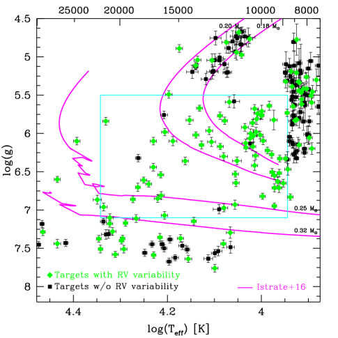
Figure 1: Effective temperature $T_{\rm eff}$ versus surface gravity $\log{g}$ for all 230 candidates with $>$3 spectroscopic observations. Green points are candidates with significant radial velocity variability; the binaries. Magenta lines are selected WD tracks for halo progenitors from Istrate et al. (2016), with the shell flash loops in $>$0.25 $M_{\odot}$ tracks clipped for the sake of clarity. The cyan box marks the clean ELM WD sample, a region in which observations are complete in the range $15<g_{0}<20$ mag in the SDSS footprint.

2.4 Stellar Atmosphere Fits

We perform stellar atmosphere fits as described in previous ELM Survey papers. We fit the summed, rest-frame spectra of each candidate to a grid of pure hydrogen atmosphere models that span 4,$000~{}{\rm K}<T_{\rm eff}<35$,000 K and $4.5<\log{g}<9.5$ (Gianninas et al., 2011, 2014, 2015) and that include the Stark broadening profiles from Tremblay & Bergeron (2009). We then apply the Tremblay et al. (2015) three-dimensional stellar atmosphere model corrections if needed. We present the corrected stellar atmosphere parameters for all 230 candidates in the electronic version of Table 2, but limit the print version of Table 2 to the 25 well-constrained new binaries.

Figure 1 plots the distribution of $T_{\rm eff}$ and $\log{g}$ for the 230 candidates with multi-epoch observations. The candidates with significant radial velocity variability – the binaries – are marked with green diamonds. Magenta lines are theoretical evolutionary tracks from Istrate et al. (2016) for halo ($Z=0.001$ progenitor) WDs with masses ranging from 0.18 $M_{\odot}$ to 0.32 $M_{\odot}$. We clip the loops due to shell flashes – the discontinuities in the higher-mass tracks – for purpose of illustration.

The distribution of points in Figure 1 reflects our target selection convolved with our follow-up approach. Our multi-epoch observations span candidates with $4.5<\log{g}<7.5$, but the follow-up is only complete for candidates with $5<\log{g}<7$. The Survey contains many false-positives around $\log{g}\sim 5$ because the underlying color selection pushes up against the locus of normal A-type stars – field blue stragglers – at low gravities. At higher gravities, the color selection pushes up against the locus of normal DA-type WDs.

In Figure 1, candidates hotter than 12,000 K primarily come from the HVS Survey target selection. Subdwarf B stars, objects found in the range 25$,000<T_{\rm eff}<40,$000 K and $5<\log{g}<6$ (Heber, 2009), are deliberately excluded from the target selection (thus the empty upper left corner of Figure 1). Candidates cooler than 12,000 K primarily come from the ELM Survey target selection; the band of subdwarf A-type stars at $<$9,000 K is notable. The band of low-gravity objects around 12,000 K is also heavily contaminated by field blue stragglers (see discussion of Gaia results below).

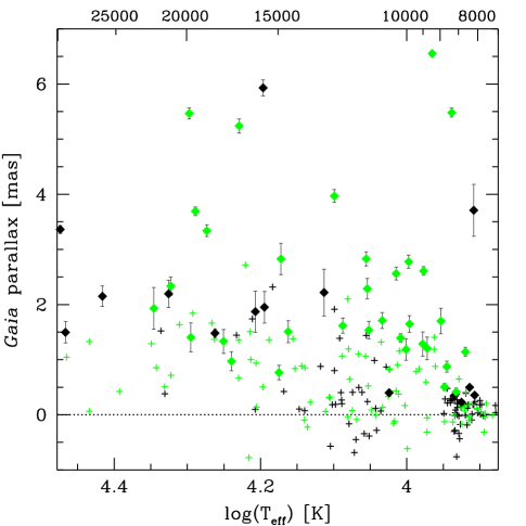
Figure 2: Gaia parallax vs. temperature, plotted on the same scale as Figure 1. Solid diamonds with errorbars mark candidates with $\pi/\sigma_{\pi}>$5; plus signs mark everything else. Green colors mark binaries. Dotted line marks zero parallax.

2.5 Gaia Astrometry

We cross-match the 230 candidates against Gaia Data Release 2 (DR2) on the basis of position and apparent magnitude. We find matches for all 230 candidates, although 8 candidates lack 5-parameter (position, proper motion, and parallax) solutions. Table 2 presents the Gaia values for the sample. For the eight objects without Gaia DR2 measurements, we present proper motions from Gaia-PanStarrs1 (Tian et al., 2017).

Parallax provides a direct constraint on the stellar nature of the candidates. Figure 2 plots the distribution of parallax versus temperature for all 222 candidates with 5-parameter Gaia DR2 measurements. We apply the parallax zero-point offset 0.029 mas recommended by the Gaia team (Lindegren et al., 2018). For the sake of clarity, we draw errorbars only for those candidates with parallax values greater than 5 times the parallax error, $\pi/\sigma_{\pi}>5$, the quality threshold used by the Gaia team (Lindegren et al., 2018). The 53 candidates with $\pi/\sigma_{\pi}>5$ are marked as solid diamond in Figure 2; everything else is marked as a plus sign.

Candidates with few mas parallaxes, or few hundred pc distances, are likely nearby WDs and are present at all temperatures in our sample. Candidates with approximately zero parallax are much more distant and unlikely to be WDs. The zero parallax objects are clumped around 12,000 K and 8,500 K, and correspond to the $\log{g}<5.5$ and $T_{\rm eff}<9,$000 K groups of candidates in Figure 1.

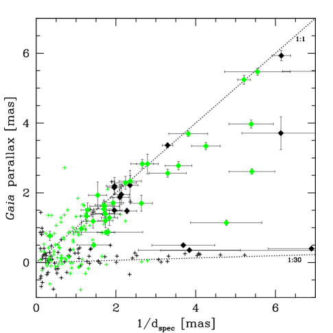
Figure 3: Gaia parallax vs. inverse spectrophotometric distance. Symbols are the same as Figure 2. Dotted lines are the 1:1 and 1:30 parallax ratio lines. The parallax distribution suggests that about half of the candidates are nearby WDs and half are distant subdwarf A (field blue straggler) stars.

Table 2: Measured and Derived Parameters

Object	R.A.	Decl.	$g_{0}$	$T_{\rm eff}$	$\log g$	WD	ELM	Clean	Disk	Mass(WD=1)	$M_{g}$(WD=1)	$d_{helio}$(WD=1)	Plx	$\mu_{\rm RA}$	$\mu_{\rm Dec}$	Gaia DR2 Source ID
	(h:m:s)	(d:m:s)	(mag)	(K)	(cm s-2)					($M_{\odot}$)	(mag)	(kpc)	(mas)	(mas yr-1)	(mas yr-1)
J0027$-$1516	0:27:51.748	$-$15:16:26.57	$17.131\pm 0.025$	$10801\pm 200$	$6.127\pm 0.052$	1	1	1	1		$8.56\pm 0.13$	$0.518\pm 0.071$	$1.7115\pm 0.1444$	$-11.936\pm 0.2882$	$-10.126\pm 0.1991$	2374553930375154944
J0042$+$3103	0:42:07.253	31:03:29.45	$18.005\pm 0.016$	$9507\pm 100$	$6.274\pm 0.048$	1	1	1	1		$9.32\pm 0.11$	$0.545\pm 0.062$	$1.2825\pm 0.2221$	$-14.913\pm 0.3631$	$2.2823\pm 0.2752$	360595902165353472
J0050$+$2147	0:50:46.851	21:47:25.66	$20.061\pm 0.024$	$14218\pm 250$	$5.826\pm 0.053$	1	1	0	0		$7.12\pm 0.15$	$4.102\pm 0.623$	$0.8389\pm 0.8569$	$2.9275\pm 1.7905$	$-11.545\pm 2.0285$	2801934821646404480
J0124$+$3908	1:24:59.733	39:08:04.43	$18.285\pm 0.013$	$29175\pm 330$	$7.286\pm 0.047$	1	0	0	1		$8.68\pm 0.12$	$0.833\pm 0.104$	$1.0446\pm 0.2482$	$4.2722\pm 0.4607$	$-3.4473\pm 0.4473$	323571256848983552
J0130$+$5321	1:30:58.174	53:21:38.37	$14.288\pm 0.009$	$9231\pm 100$	$6.627\pm 0.056$	1	1	0	1		$10.26\pm 0.10$	$0.085\pm 0.009$	$6.5549\pm 0.0515$	$61.1420\pm 0.0918$	$-86.462\pm 0.0855$	407508116250828800
J0147$+$0113	1:47:20.465	1:13:58.28	$20.216\pm 0.022$	$9383\pm 100$	$6.947\pm 0.040$	1	1	0	0		$10.76\pm 0.09$	$0.809\pm 0.075$	$-0.3146\pm 0.8756$	$3.1155\pm 1.4860$	$-52.577\pm 1.6687$	2511132447278844928
J0151$+$1812	1:51:20.679	18:12:47.95	$19.604\pm 0.027$	$8879\pm 90$	$6.328\pm 0.050$	1	1	1	1		$9.90\pm 0.10$	$0.933\pm 0.098$	$-0.1289\pm 0.4323$	$13.9995\pm 0.9192$	$-2.7449\pm 0.7981$	92092035925893888
J0212$+$2657	2:12:16.043	26:57:53.52	$19.419\pm 0.031$	$9163\pm 100$	$6.518\pm 0.049$	1	1	1	0		$10.14\pm 0.11$	$0.804\pm 0.089$	$1.4057\pm 0.4510$	$-9.4283\pm 0.8561$	$-13.408\pm 0.7127$	107127651277641472
J0441$-$0547	4:41:32.625	$-$5:47:34.95	$18.310\pm 0.016$	$12732\pm 330$	$5.045\pm 0.086$	0	0	0	$\cdots$		$5.40\pm 0.26$	$4.733\pm 1.252$	$0.3092\pm 0.2872$	$4.8286\pm 0.4549$	$-6.2472\pm 0.3931$	3200233905240195968
J0923$-$1218	9:23:50.319	$-$12:18:24.00	$16.325\pm 0.004$	$19455\pm 210$	$7.170\pm 0.041$	1	0	0	1		$9.23\pm 0.13$	$0.262\pm 0.034$	$3.6920\pm 0.0792$	$-17.484\pm 0.1362$	$12.7521\pm 0.1185$	5738500791959712768
J1021$+$0543	10:21:53.117	5:43:22.28	$19.360\pm 0.017$	$18314\pm 220$	$6.703\pm 0.054$	1	1	1	0		$8.60\pm 0.12$	$1.420\pm 0.178$	$1.3622\pm 0.6033$	$-10.721\pm 1.1203$	$-11.711\pm 0.8998$	3861429723729285376
J1048$-$0000	10:48:26.862	$-$0:00:56.81	$18.261\pm 0.023$	$8484\pm 90$	$5.831\pm 0.051$	1	1	0	1		$9.01\pm 0.25$	$0.707\pm 0.175$	$0.6502\pm 0.3045$	$-3.0858\pm 0.4047$	$-5.3089\pm 0.3125$	3806330138044722176
J1115$+$0246	11:15:27.310	2:46:21.86	$18.835\pm 0.018$	$27182\pm 450$	$7.439\pm 0.056$	1	0	0	0		$9.06\pm 0.10$	$0.899\pm 0.091$	$1.3282\pm 0.4507$	$-13.836\pm 0.7201$	$-6.2443\pm 0.4607$	3811751005247652352
J1138$-$0035	11:38:40.679	$-$0:35:32.17	$14.090\pm 0.021$	$31614\pm 330$	$5.627\pm 0.045$	0	0	0	$\cdots$		$5.30\pm 0.12$	$0.571\pm 0.072$	$0.8649\pm 0.0630$	$-8.4262\pm 0.1173$	$-25.372\pm 0.0699$	3794197787442075008
J1401$-$0817	14:01:18.801	$-$8:17:23.43	$16.456\pm 0.017$	$8813\pm 90$	$5.731\pm 0.048$	1	1	1	0		$7.73\pm 0.48$	$0.555\pm 0.268$	$0.8736\pm 0.1002$	$-5.0012\pm 0.1759$	$-79.203\pm 0.1322$	3616216816596857984
J1545$+$4301	15:45:21.102	43:01:41.85	$18.998\pm 0.021$	$9707\pm 110$	$6.222\pm 0.043$	1	1	1	1		$9.13\pm 0.10$	$0.939\pm 0.100$	$0.7866\pm 0.2128$	$0.4223\pm 0.3776$	$0.5518\pm 0.4952$	1396245695576598272
J1638$+$3500	16:38:26.274	35:00:12.03	$14.561\pm 0.015$	$37250\pm 570$	$8.070\pm 0.050$	1	0	0	1		$9.49\pm 0.44$	$0.103\pm 0.046$	$6.8981\pm 0.0321$	$-35.102\pm 0.0512$	$8.9790\pm 0.0652$	1327577144269234176
J1708$+$2225	17:08:16.358	22:25:51.07	$19.106\pm 0.015$	$22343\pm 450$	$6.865\pm 0.059$	1	0	0	1		$8.29\pm 0.08$	$1.612\pm 0.130$	$1.2867\pm 0.4295$	$-1.7690\pm 0.6684$	$3.5902\pm 0.6154$	4568269229123390336
J1738$+$2927	17:38:35.467	29:27:50.63	$19.309\pm 0.017$	$12018\pm 230$	$6.972\pm 0.051$	1	1	1	1		$10.01\pm 0.11$	$0.780\pm 0.090$	$1.1932\pm 0.3759$	$-9.8331\pm 0.5359$	$6.1181\pm 0.7191$	4595849099618519680
J2147$+$1859	21:47:28.476	18:59:59.76	$19.580\pm 0.022$	$9618\pm 110$	$5.639\pm 0.059$	1	1	1	1		$7.87\pm 0.13$	$2.199\pm 0.286$	$0.8328\pm 0.6796$	$-0.7578\pm 0.9284$	$-2.6692\pm 1.1753$	1780334519094674304
J2245$+$0750	22:45:21.283	7:50:48.74	$19.635\pm 0.022$	$10782\pm 110$	$6.184\pm 0.056$	1	1	1	1		$8.69\pm 0.14$	$1.547\pm 0.213$	$0.1356\pm 0.7483$	$9.0727\pm 1.2676$	$-3.2587\pm 1.0968$	2712813082023657600
J2317$+$0602	23:17:57.418	6:02:52.09	$19.494\pm 0.035$	$12043\pm 160$	$7.441\pm 0.052$	1	0	0	1		$10.76\pm 0.09$	$0.558\pm 0.054$	$2.1029\pm 0.6595$	$7.1097\pm 2.4904$	$-2.1619\pm 0.9112$	2664126329188074240
J2332$+$0427	23:32:46.564	4:27:35.20	$18.022\pm 0.014$	$11967\pm 160$	$5.834\pm 0.048$	1	1	1	0		$8.06\pm 0.18$	$1.087\pm 0.199$	$0.6446\pm 0.2393$	$14.4921\pm 0.4318$	$-13.927\pm 0.2615$	2660056212019666688
J2339$+$2024	23:39:53.667	20:24:44.84	$18.244\pm 0.014$	$8019\pm 90$	$5.263\pm 0.059$	0	0	0	$\cdots$		$7.53\pm 0.08$	$1.387\pm 0.107$	$0.1180\pm 0.2031$	$-0.3283\pm 0.3558$	$-2.3290\pm 0.2247$	2826170531823332096
J2339$-$0347	23:39:38.450	$-$3:47:34.51	$18.542\pm 0.025$	$16047\pm 260$	$5.982\pm 0.047$	1	1	1	1		$7.28\pm 0.12$	$1.882\pm 0.223$	$0.1387\pm 0.6493$	$-5.3204\pm 1.1572$	$-3.1589\pm 0.7429$	2639275992010565376

Note. — $g_{0}$ is de-reddened SDSS $g$-band apparent magnitude, except for 5 cases when it is derived from PanStarrs $g$ or Gaia $G$. Measured $T_{\rm eff}$ and $\log{g}$ values are corrected for 3D effects following Tremblay et al. (2015). Classifications are set to 1 if true or 0 if false, i.e. WD=1 indicates a WD, ELM=1 indicates an ELM WD, Clean=1 indicates an ELM WD in the clean sample, and disk=1 indicates an object that orbits in the disk. WD mass, absolute $g$-band magnitude $M_{g}$, and distance are derived using the models of Althaus et al. (2013) and Istrate et al. (2016), but are only valid for objects marked WD=1. For the eight candidates without Gaia 5-parameter solutions, we list proper motions from Gaia-PanStarrs1 (Tian et al., 2017). This table is available in its entirety in machine-readable and Virtual Observatory forms in the online journal. The 25 well-constrained new binaries are shown here for guidance regarding form and content.

2.6 White Dwarf Parameters

For every candidate, we interpolate its $T_{\rm eff}$ and $\log{g}$ measurements through WD evolutionary tracks to estimate its putative WD mass and luminosity. We use Istrate et al. (2016) tracks for ELM WDs because they are computed for both solar metallicity and halo metallicity progenitors. A significant fraction of the observed ELM WDs belong to the halo. We also use Althaus et al. (2013) tracks, and in one case Tremblay et al. (2011) tracks, to cover the full range of temperature and surface gravity of our sample.

The Istrate et al. (2016) tracks overlap the observations in the region 8,$800~{}{\rm K}<T_{\rm eff}<22,$000 K and $\log{g}<7.1$ (the cyan box in Figure 1). This motivates us to refer to these candidates as ELM WDs. In this region, we apply Istrate et al. (2016) $Z=0.02$ tracks with rotation to disk objects and the $Z=0.001$ tracks with rotation to halo objects. We apply Althaus et al. (2013) tracks to everything else, except for the more massive WD J1638+3500 which requires Tremblay et al. (2011) tracks. The WD masses derived from the Istrate et al. (2016) and Althaus et al. (2013) tracks differ by 0.00$\pm$0.012 $M_{\odot}$ in their region of overlap. We thus compute mass errors by propagating the $T_{\rm eff}$ and $\log{g}$ uncertainties through the tracks and adding $\pm$0.01 $M_{\odot}$ in quadrature.

We then compute heliocentric distances, $d$, using de-reddened apparent SDSS $g$-band magnitude, $g_{0}$, and the absolute magnitude $M_{g}$ derived from the tracks, $d=10^{((g_{0}-M_{g})/5-2)}$ kpc. Applying the full reddening correction may be incorrect for the nearest WDs; however the median WD in our sample is 0.8 kpc distant and has low $E(B-V)=0.031$ mag reddening.

Figure 3 compares Gaia parallax to the inverse of our spectrophotometric distance estimate. We see two bands in Figure 3. The band of candidates near the 1:30 ratio line in Figure 3 are approximately 30 times more distant, or $\sim$1,000 times more luminous, than we estimate from WD models. Since $T_{\rm eff}$ should be accurately measured, we conclude that these candidates have radii $\sim$30 times larger than WDs. The candidates near the 1:30 ratio line are thus likely metal-poor stars at kpc distances in the halo, objects traditionally called field blue stragglers at these temperatures.

The candidates scattered around the diagonal 1:1 ratio line in Figure 3 are likely WDs. There are also some candidates just below the 1:1 ratio line which notably have $T_{\rm eff}<9,$000 K. If we again assume temperature is robust, these cool WDs just below the 1:1 ratio line can be explained by either $\sim$1.7$\times$ inflated radii or $\sim$0.5 dex systematic $\log{g}$ errors. The latter explanation is consistent with our previously published systematic error estimate for pure hydrogen models at $<$9,000 K temperatures (Brown et al., 2017a).

For the candidates with $T_{\rm eff}>9,$500 K, the ELM WD models of Istrate et al. (2016) and Althaus et al. (2013) provide remarkably accurate measures of luminosity. The mean parallax ratio of the 35 candidates with $\pi/\sigma_{\pi}>$5 and 9,$500<T_{\rm eff}<30,$000 K, after clipping a single field blue straggler interloper, is $0.97\pm 0.04$.

2.7 Clean ELM WD Sample

We define a clean sample of WDs, and of ELM WDs, on the basis of our stellar atmosphere measurements and Gaia parallax. The subset of our sample with $\pi/\sigma_{\pi}>$5 demonstrate that $T_{\rm eff}>9,$000 K and $\log{g}>5.5$ candidates are a clean set of WDs. Metal-poor main sequence stars at the same temperatures have distinct $\log{g}\leq 4.7$ (e.g., Marigo et al., 2017).

Thus we start building our clean sample of WDs from the 115 candidates with $T_{\rm eff}>9,$000 K and $\log{g}>5.5$. We remove 5 objects that do not belong: the sdB star, and four candidates with $\pi/\sigma_{\pi}>$5 and distance estimates that differ by more than 3$\times$.

We then add candidate WDs with $T_{\rm eff}<9,$000 K or $\log{g}<5.5$ on the basis of parallax and binary orbital period. Excluding the sdA pulsator J1355+1956 (Bell et al., 2017), six candidates have $\pi/\sigma_{\pi}>$5 and distance estimates that agree to within a factor of 3. Interestingly, two-thirds are short-period binaries. There are an additional six candidates with significant $k>100$ km s^-1 orbital motion and short $P<0.27$ d periods. Orbits with $P<0.27$ d exclude metal-poor A-type stellar radii on basis of Padova tracks (Marigo et al., 2017) and the Roche lobe criterion (Eggleton, 1983). Summed together, the result is a sample of 122 likely WDs. We label these objects WD=1 in Table 2.

We identify ELM WDs as those WDs with $M<0.3$ $M_{\odot}$, in other words, the WDs that overlap the ELM WD tracks (Althaus et al., 2013; Istrate et al., 2016). There are 79 ELM WDs in our sample by this definition. Two WDs with masses just above 0.3 $M_{\odot}$, J0822+3048 and J0935+4411, are now excluded. However, some of the ELM WDs included in our definition are drawn from outside the SDSS survey footprint, or have apparent magnitudes outside our primary magnitude selection.

Thus we additionally define a clean ELM WD sample: ELM WDs in the de-reddened magnitude range $15<g_{0}<20$, located in the SDSS footprint, with 8,$800~{}{\rm K}<T_{\rm eff}<22,$000 K and $5.5\leq\log{g}\leq 7.1$. We choose this range to maximize the overlap between the ELM WD tracks and the observations, and to minimize contamination (see Figure 1). This excludes ancillary candidates we identified in the TESS Input Catalog, the Edinburgh-Cape Survey, and the LAMOST catalog so that the photometric and spatial selection is uniform. We use inclusive $\log{g}$ boundaries to include the eclipsing ELM WD binary J0751$-$0141 (Kilic et al., 2014b). The clean sample of ELM WDs contains 62 objects and is essentially complete within our selection criteria.

Table 2 summarizes our classifications. The values of each column are set to 1 if true or 0 if false, i.e. ELM=1 indicates an ELM WD, and Clean=1 indicates an ELM WD in the clean sample. Note that the clean ELM WD sample defined here differs from our previous papers: we intentionally exclude the coolest and lowest-gravity ELM WD candidates so as to minimize contamination from other stellar populations.

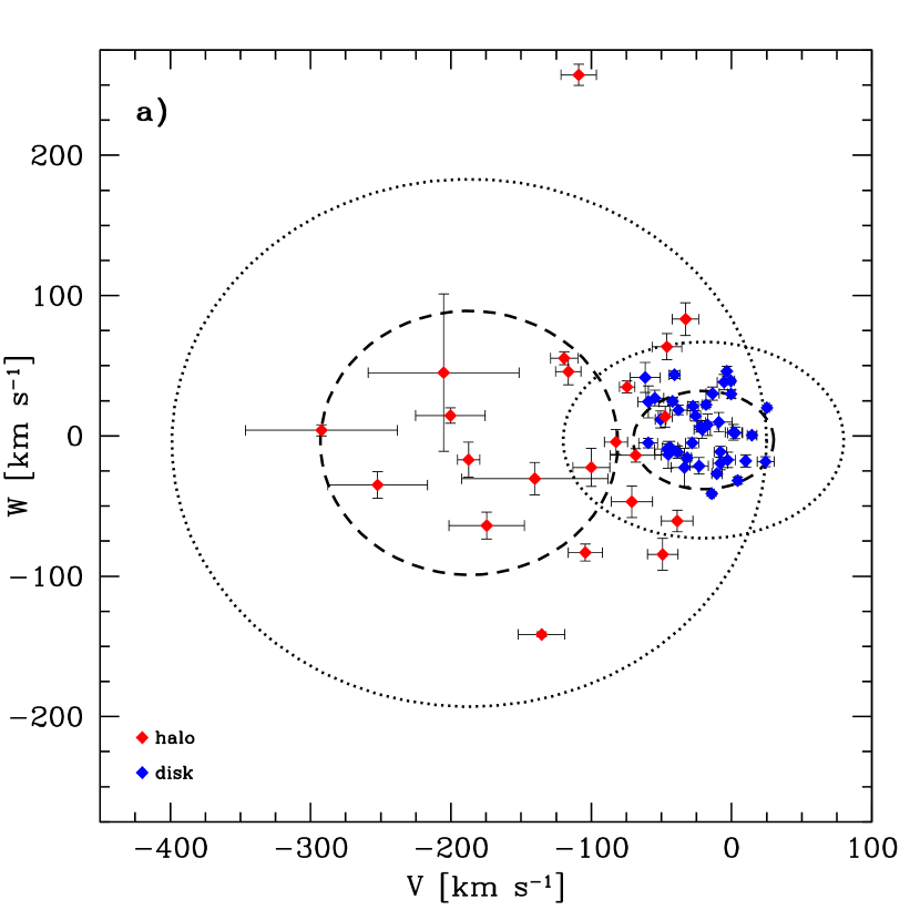
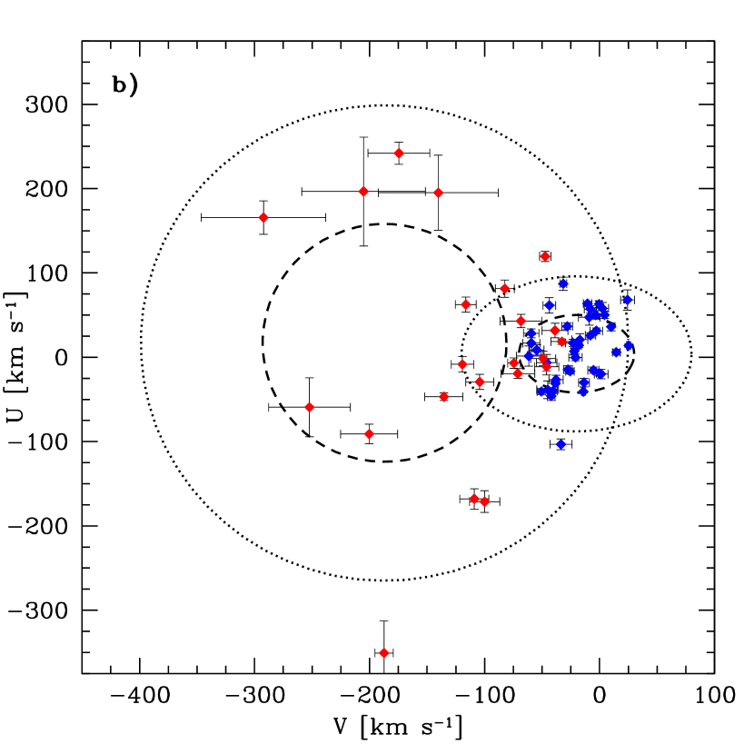
Figure 4: Velocity distribution of the clean ELM WD sample, plotted in Galactic cartesian velocity components $U$ (in the direction of the Galactic center), $V$ (in the direction of Galactic rotation), and $W$ (in the direction of the north Galactic pole). For comparison are the 1$\sigma$ (dashed) and 2$\sigma$ (dotted) velocity ellipsoid values for stellar thick disk and halo populations (Chiba & Beers, 2000). We classify 37% of the sample as halo (red points) and 63% as disk (blue points).

2.8 White Dwarf Disk/Halo Membership

We classify the disk/halo membership for the clean ELM WD sample on the basis of space velocity. Previously, we found that 37% of ELM WD binaries in our sample orbit in the halo (Gianninas et al., 2015; Brown et al., 2016b). Gaia proper motions provide an order-of-magnitude improvement in accuracy compared to previous work.

We compute tangential velocity from the product of Gaia proper motion and spectrophotometric distance, because spectrophotometric distance has smaller uncertainties than parallax for most of the clean ELM WD sample. We measure systemic radial velocity directly, and correct it for ELM WD gravitational redshift. The median tangential and systemic radial velocity errors in the clean ELM WD sample are 20 km s^-1 and 4 km s^-1, respectively.

We calculate Galactic $UVW$ velocities assuming a circular motion of 235 km s^-1 (Reid et al., 2009) and the solar motion of Schönrich et al. (2010), and determine disk/halo membership on the basis of ELM WD space velocity and spatial location using equations 2–8 in Brown et al. (2016b). This approach yields 35% (22/62) halo objects and 65% (40/62) disk objects in the clean ELM WD sample, essentially the same fraction as before. We present the disk/halo classifications for all 122 WDs in Table 2.

Figure 4 plots the distribution of Galactic $U$, $V$, and $W$ velocity components for the clean ELM WD sample. Disk objects are drawn in blue, halo objects are drawn in red. For comparison, we draw the velocity ellipsoid values of the halo and thick disk from Chiba & Beers (2000).

Interestingly, disk and halo ELM WDs exhibit statistically identical distributions of other parameters. Disk and halo ELM WDs overlap in $T_{\rm eff}$ and $\log{g}$ space. A two-sample Anderson-Darling test (Scholz & Stephens, 1987) on the ELM WD mass distribution, semi-amplitude distribution, and orbital period distribution all have p-values around 0.4. We conclude that ELM WDs share similar binary properties, described below, regardless of their disk/halo origin.

3 BINARIES

We now focus on the binaries. We present orbital parameters for 128 binaries in the completed ELM Survey, including 29 published here for the first time (25 of which are well-constrained). We use follow-up radial velocity measurements to rule out period aliases in previously published binaries, and use X-ray and radio observations to place constraints on the presence of millisecond pulsar companions around previously published binaries. We close with an optical light curve for the new $P=0.048$ d ELM WD binary J1738+2927.

Figure 5: Radial velocities phased to the best-fit orbital solutions for the 25 well-constrained new binaries.

3.1 Velocity Variability

We identify binaries among the low mass WD candidates on the basis of radial velocity variability. Radial velocities are measured with the cross-correlation technique using the full wavelength range of the spectra, as described in Section 2.3. A pair of radial velocities is often sufficient to detect the median $P=6$ h, $k=200$ km s^-1 binary in our sample. However, we find that 4 to 7 observations are necessary to perform a significant test for orbital motion. We use the F-test to quantify whether the variance of the observations, given measurement errors, is consistent with a constant velocity. Candidates with p-values $<0.01$ are inconsistent with constant velocity, in other words, they are likely binaries.

Sensitivity tests show that our cadence of observations and measurement errors have a 99% likelihood of detecting binaries with semi-amplitudes $k>100$ km s^-1 and $P<2$ d (Brown et al., 2016a). We acquire a median 21 observations per binary. Observations are separated by minutes to hours over the course of multiple observing runs; the exact cadence of observations depends on the period of the binary and where it was placed on the sky during our observing runs.

We find that 128 of the 230 candidates have statistically significant velocity variability. These binaries are drawn with green symbols in Figures 1–3. Of the 128 velocity variable objects, 99 are published in our previous papers and 29 are new (25 of which are well-constrained binaries).

Table 3: Binary Parameters

Object	$N_{\rm obs}$	$P$	$k$	$\gamma$	$M_{\rm 2,min}$	$\log{\tau_{\rm,max}}$	alias?	$\Delta\chi^{2}_{\rm alias}$	$P_{\rm alias}$	$h_{c}\sqrt{(4~{}{\rm yr})f}$
		(d)	(km s-1)	(km s-1)	($M_{\odot}$)	(yr)			(days)	($\times 10^{-21}$)
J0027$-$1516	18	$0.42458\pm 0.00014$	$155.4\pm 6.3$	$-42.4\pm 6.9$	0.36	10.79	0	64.17	0.29780	$1.4^{+2.0}_{-0.6}$
J0042$+$3103	16	$0.29725\pm 0.00018$	$204.2\pm 5.2$	$-48.6\pm 5.5$	0.49	10.28	0	338.9	0.22913	$2.4^{+3.3}_{-0.9}$
J0050$+$2147	15	$0.36059\pm 0.00002$	$183.7\pm 6.6$	$-138.9\pm 10.9$	0.46	10.51	0	55.84	0.05355	$0.26^{+0.36}_{-0.10}$
J0124$+$3908	16	$1.29211\pm 0.00433$	$127.0\pm 9.9$	$1.8\pm 11.3$	0.69	11.54	1	0.74	0.22477	$0.77^{+0.92}_{-0.30}$
J0130$+$5321	32	$0.19205\pm 0.00020$	$209.1\pm 5.1$	$-105.8\pm 8.8$	0.40	9.81	0	433.6	0.23789	$24^{+35}_{-10}$
J0147$+$0113	19	$1.30338\pm 0.00483$	$145.9\pm 15.7$	$-107.9\pm 15.2$	0.74	11.74	1	6.95	0.57599	$0.50^{+0.57}_{-0.19}$
J0151$+$1812	19	$0.14812\pm 0.00001$	$259.8\pm 3.5$	$-8.1\pm 3.1$	0.47	9.54	0	154.3	0.13020	$2.8^{+3.8}_{-1.1}$
J0212$+$2657	17	$0.44908\pm 0.00197$	$202.0\pm 11.5$	$-107.1\pm 9.3$	0.62	10.70	0	78.62	0.31291	$1.1^{+1.4}_{-0.4}$
J0441$-$0547	15	$1.31997\pm 0.00060$	$242.7\pm 18.1$	$-155.9\pm 11.7$	2.28	11.51	1	6.54	1.55179	$\cdots$
J0923$-$1218	51	$0.14896\pm 0.00002$	$117.0\pm 3.7$	$29.4\pm 2.7$	0.19	9.56	0	64.73	0.17512	$31^{+28}_{-10}$
J1021$+$0543	20	$1.24995\pm 0.00410$	$95.6\pm 11.6$	$-30.0\pm 13.6$	0.33	11.98	0	14.99	1.38071	$0.17^{+0.25}_{-0.07}$
J1048$-$0000	20	$0.12063\pm 0.00001$	$312.8\pm 8.1$	$45.7\pm 6.1$	0.62	9.18	0	751.1	0.10763	$6.3^{+7.7}_{-2.6}$
J1115$+$0246	10	$0.12405\pm 0.00004$	$139.9\pm 12.2$	$90.0\pm 8.1$	0.26	9.15	1	0.39	0.14175	$16^{+14}_{-5}$
J1138$-$0035	36	$0.20769\pm 0.00002$	$155.0\pm 4.9$	$9.9\pm 3.9$	0.25	10.05	0	74.25	0.17189	$\cdots$
J1401$-$0817	35	$0.11299\pm 0.00001$	$346.2\pm 2.7$	$198.7\pm 2.0$	0.79	8.93	0	6885	0.12746	$13^{+19}_{-7}$
J1545$+$4301	25	$0.30931\pm 0.00016$	$154.8\pm 4.1$	$18.2\pm 4.0$	0.30	10.50	0	111.0	0.45533	$0.94^{+1.45}_{-0.37}$
J1638$+$3500	66	$0.90606\pm 0.00031$	$89.5\pm 4.4$	$-17.5\pm 4.1$	0.45	11.09	0	24.60	0.47468	$30^{+30}_{-12}$
J1708$+$2225	17	$0.23735\pm 0.00024$	$115.5\pm 8.5$	$-6.5\pm 6.6$	0.22	10.07	1	8.56	1.00795	$2.3^{+2.3}_{-0.8}$
J1738$+$2927	17	$0.04770\pm 0.00011$	$372.7\pm 13.2$	$-11.9\pm 12.8$	0.55	7.97	0	66.08	0.05274	$24^{+29}_{-9}$
J2147$+$1859	20	$0.12879\pm 0.00002$	$198.3\pm 6.6$	$-67.9\pm 5.5$	0.27	9.56	0	153.0	0.17977	$0.94^{+1.48}_{-0.40}$
J2245$+$0750	18	$0.39664\pm 0.00102$	$220.5\pm 10.1$	$-34.2\pm 11.7$	0.70	10.50	0	73.41	0.65750	$0.77^{+0.89}_{-0.28}$
J2317$+$0602	20	$0.86702\pm 0.00133$	$100.7\pm 7.3$	$-34.2\pm 12.2$	0.38	11.32	1	5.47	1.27191	$1.4^{+1.8}_{-0.6}$
J2332$+$0427	24	$0.36792\pm 0.00009$	$212.5\pm 4.9$	$-7.0\pm 3.5$	0.61	10.44	0	420.6	0.51537	$1.1^{+1.4}_{-0.4}$
J2339$+$2024	14	$0.79578\pm 0.00008$	$106.3\pm 5.0$	$157.3\pm 3.7$	0.28	11.60	0	56.46	0.43107	$\cdots$
J2339$-$0347	19	$0.67069\pm 0.00078$	$139.7\pm 6.0$	$31.2\pm 10.9$	0.41	11.26	0	73.22	1.37843	$0.26^{+0.37}_{-0.10}$

Note. — $N_{\rm obs}$ is the number of spectroscopic observations. $P$ is the binary orbital period. $k$ is the radial velocity semi-amplitude. $\gamma$ is the systemic velocity corrected for gravitational redshift. $M_{\rm 2,min}$ is the minimum mass of the secondary. $\tau_{\rm,max}$ is the maximum gravitational merger timescale. Binaries with significant period aliases have alias=1 if true or 0 if false. $\Delta\chi^{2}_{\rm alias}$ is the $\chi^{2}$ at $P_{\rm alias}$ relative to the global $\chi^{2}$ minimum. $h_{c}$ is the characteristic strain and $\sqrt{(4~{}{\rm yr})f}$ is the S/N boost from the number of cycles during the LISA observation time (the values plotted in Figure 10). This table is available in its entirety in machine-readable and Virtual Observatory forms in the online journal. The 25 well-constrained new binaries are shown here for guidance regarding form and content.

3.2 Binary Orbital Elements

We calculate orbital elements as described in previous ELM Survey papers. We start by using the summed, rest-frame spectrum of each target as its own cross-correlation template to maximize the velocity precision. We then minimize $\chi^{2}$ for a circular orbit fit following the code of Kenyon & Garcia (1986). We find that our cross-correlation approach underestimates velocity error, however. To obtain a reduced $\chi^{2}\simeq 1$ requires adding a median 15 km s^-1 velocity error in quadrature to the measurements. Thus we estimate orbital element errors by re-sampling the velocities with the extra error added in quadrature and re-fitting the orbital solution 10,000 times. This Monte Carlo approach samples the $\chi^{2}$ space in a self-consistent way. We report orbital element errors derived from the 15.9% and 84.1% percentiles of the distributions in Table 3. Systemic velocities are corrected for gravitational redshift using the WD parameters in Table 2.

Figure 5 plots the radial velocities of the 25 well-constrained new binaries, phased to their best-fit orbits. Four other objects have significant velocity variability but are not WDs on the basis of their parallax, so we did not pursue a full set of observations.

The 25 well-constrained new binaries with robust orbital solutions are mostly low mass WD binaries, including two previously unknown binaries that we selected as additional low mass WD candidates: we found J0923$-$1218 = WD 0921$-$120 in the Edinburgh-Cape Survey (Kilkenny et al., 1997), and J0130+5321 = GD 278 in the TESS bright WD catalog (Raddi et al., 2017). Two objects are not low mass WD binaries but we publish the observations for completeness: J1638+3500 is a hot 0.7 $M_{\odot}$ WD we observed for the SWARMS survey (Badenes et al., 2009), and J1138$-$0035 turns out to be a hot subdwarf B star (Geier et al., 2011). In 6 cases the orbital solutions have period aliases due to insufficient sampling (as seen in J1115+0246 and J1708+2225) and/or uneven phase coverage (as seen in J0124+3908 and J0441$-$0547).

Period aliases, not statistical errors, are the largest source of uncertainty in the orbital solutions. We consider an object to have a significant period alias if its orbital elements have local $\chi^{2}$ minima within $\Delta\chi^{2}=13.3$ of the global $\chi^{2}$ minimum (Press et al., 1992). On this basis, 27% (34/128) of the binaries have significant period aliases. Many of the binaries with period aliases are field blue stragglers that we chose not to continue observing; only 15% (15/98) of the WD binaries have period aliases.

For completeness, we present the strongest period alias, and its $\Delta\chi^{2}$ value with respect to the global minimum, for all 128 binaries in Table 3. The aliases are found equally at longer and shorter periods. The exceptions are low semi-amplitude field blue stragglers. These objects often have short $\sim$1 h period aliases trivially matched to the cadence of observations, but their low semi-amplitudes suggest the long period solution is likely correct.

We obtained additional observations that eliminated period aliases for 11 previously published WD binaries. In seven cases, the originally published period was correct and the orbital solution is unchanged. In four cases, the alias was correct: J1005+0542 is $P=4.5$ h, J1422+4352 is $P=14.9$ h, J1439+1002 is $P=18.6$ h, and J1557+2823 is $P=6.9$ h.

Figure 6 plots the overall distribution of velocity semi-amplitude, $k$, versus orbital period, $P$, for all 128 binaries. Binaries with period aliases are drawn with a single open symbol at their best-fit period. For the purpose of guidance, not analysis, we draw dashed lines that indicate the approximate companion mass calculated for $M_{1}=0.2$ $M_{\odot}$ and inclination $i=60\arcdeg$. The lines in Figure 6 are thus only relevant to the ELM WD systems. Dotted lines indicate the approximate gravitational wave merger timescale calculated with the same assumptions. Most of the binaries with period aliases are field blue stragglers that have $k<75$ km s^-1 or $P>30$ h. The outlier at $(P,k)=(1.3$ d, 243 km s^-1), J0441$-$0547, has a significant period alias at 0.57 d.

In the absence of a constraint on inclination, i.e. from eclipses, our radial velocity measurements determine only the minimum mass of the companion, $M_{2}$. We list minimum $M_{2}$ mass values for the best-fit periods in Table 3. The unseen companions in the 98 binaries containing a visible WD all have minimum $M_{2}$ masses consistent with being other WDs. Spectral energy distributions provide no further constraint because, by design, we observe candidates dominated by the light of a low mass WD. The $0.97\pm 0.04$ ratio of Gaia parallax to inverse spectro-photometric distance, reported above, affirms that the companions are significantly fainter than the visible low mass WD. The low mass WDs with the largest minimum $M_{2}$ values and no period aliases are J0802$-$0955 and J0811+0225, which have $M_{2}>1.2$ $M_{\odot}$.

The minimum companion mass allows us to calculate the maximum gravitational wave merger timescale, $\tau$, of the binaries. We list the maximum merger timescales in Table 3. The values of $\tau$ range from $10^{6}$ yr to $10^{12}$ yr for our sample of binaries, as illustrated in Figure 6.

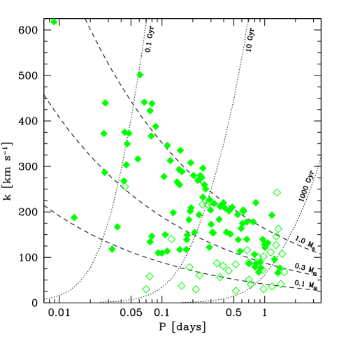
Figure 6: Observed semi-amplitude and orbital period of the 128 binaries. Binaries with period aliases are drawn with a single open symbol at their best-fit period. Statistical errors are smaller than the symbol size. For the purpose of guidance, dashed lines indicate the approximate companion mass and dotted lines indicate the corresponding gravitational wave merger timescale, calculated assuming the visible star is a 0.2 $M_{\odot}$ WD as described in the text.

3.3 Millisecond Pulsar Companions

Given the unknown inclination of our single-lined spectroscopic binaries, some of the unseen companions may be neutron stars. If true, binary evolution should naturally produce millisecond pulsars. Indeed, millisecond radio pulsars are commonly observed with low mass WD companions (Manchester et al., 2005; van Kerkwijk et al., 2005). Low mass WD+pulsar binaries have orbital periods of hours to days similar to the binaries observed here (van Kerkwijk et al., 1996; Antoniadis et al., 2013).

Millisecond pulsars have wide radio beams that cover $\sim$80% of the sky (Lyne & Manchester, 1988) and invariably show thermal X-ray emission from the heated neutron star polar caps; one pole should be visible from any observing angle due to gravitational bending of light rays (Beloborodov, 2002). Because millisecond pulsars have lifetimes exceeding $10^{10}$ years, any putative millisecond pulsar companion should be active now.

These facts motivated our follow-up radio and X-ray search for millisecond pulsar companions in the ELM Survey. Previous searches for millisecond pulsar companions to known low mass WDs, mostly in the ELM Survey, have yielded no neutron star counterparts (van Leeuwen et al., 2007; Agüeros et al., 2009b, a; Kilic et al., 2013, 2014b, 2016; Andrews et al., 2018). We present our final set of radio and X-ray observations of low mass WDs in the ELM Survey sample.

3.3.1 Radio Observations

We engaged in a long-term radio campaign using the Robert C. Byrd Green Bank Telescope (GBT) to target ELM WD candidates with the largest minimum companion masses. The results from semesters GBT/05C-041, GBT/06A-051, GBT/07C-072, and GBT/10A-046 are previously published (Agüeros et al., 2009a, b; Kilic et al., 2013). Here, we report the results for the 20 candidates observed in the semesters GBT/12A-431 and GBT/14A-438. The 20 candidates were published in previous ELM Survey papers, but their radio observations were not.

We selected targets for radio observations based on the minimum companion mass derived from the spectroscopic radial velocity curve and a Bayesian model estimate for the likelihood any particular system contains a neutron star companion (Andrews et al., 2014). We obtained GBT observations with the GUPPI backend with a central frequency of 340 MHz, using 4096 channels each with 100 MHz bandwidth. We set integration times to reach a detection threshold of 0.4 mJy kpc². Data were processed, de-dispersed, and folded using standard routines within PRESTO (Ransom et al., 2002, 2003). Our procedure searched dispersion measures as large as twice the expectation from the spectroscopic distances, using the Galactic electron density model from Cordes & Lazio (2002).

The result is a single new pulsar, PSR J0802$-$0955. However, follow-up radio observations (Andrews et al., 2018) indicate this pulsar is either a foreground or background object, unrelated to the coincident ELM WD. We therefore identify no radio pulsar companions in the ELM Survey.

Null detections place useful lower limits on inclination if we assume the secondaries have $M_{2}<1.4$ $M_{\odot}$. We list the GBT targets and their inclination constraints in the Appendix.

3.3.2 X-ray Observations

We obtained Chandra X-ray Observatory (Weisskopf et al., 2002) observations for ten low mass ELM candidates. Eight are previously published (Kilic et al., 2013, 2014b, 2016). We present the results for the final two candidates with Chandra observations, J0147+0113 and J2245+0750 here.

We observed J2245+0750 for 123 kiloseconds on 2018 September 17-22, and J0147+0113 for 13.9 kiloseconds on 2018 November 11. We placed ACIS-S at the focus, in Very Faint mode. No periods of enhanced background were seen, so we extracted spectra from 1.5″radii at the location of each WD, and fit them with a hydrogen neutron star atmosphere model (Heinke et al., 2006). We assumed a distance of 1.5 kpc for J2245+0750 and 810 pc for J0147+0113 from our spectroscopic distance estimates. We assume $N_{H}=6.35\times 10^{20}$ cm^-2 for J2245+0750 and $N_{H}$=$2.87\times 10^{20}$ cm^-2 for J0147+0113, from the Dickey & Lockman (1990) reddening estimates in these directions. We fix the assumed neutron star mass and radius to 1.4 $M_{\odot}$ and 12 km, respectively, and the temperature to $\log{T}=5.903$, the lowest observed for any millisecond pulsar in 47 Tuc (Bogdanov et al., 2006), with the normalization (thus the area of the hot spot) free.

We detect no sources at the location of either WD. We thus fit the spectra using the C-statistic (Cash, 1976), and obtain upper limits on the normalization, and thus on the X-ray luminosity. We find 90% confidence limits of $L_{X}$(0.3-8 keV)$\leq 2.6\times 10^{29}$ erg s^-1 for J2245+0750, and $\leq 2.2\times 10^{29}$ erg s^-1 for J0147+0113. These values are below the X-ray luminosities of any well-measured millisecond pulsars (Bogdanov et al., 2006; Kargaltsev et al., 2012; Forestell et al., 2014), allowing us to confidently rule out a millisecond pulsar companion in both cases. The unseen companions are likely WDs.

We can again use the null detections to place lower limits on inclination. We list the Chandra targets and their inclination constraints in the Appendix.

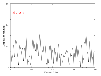
Figure 7: Optical light curve of J1738+2927 (upper panel) and Fourier transform of the light curve (lower panel). The gap in the light curve is due to zenith-crossing. The Fourier transform shows no evidence for significant variability.

3.4 Optical Light Curve

Finally, we obtained time-series optical photometry for the newly discovered $P=0.048$ d WD binary J1738+2927 on UT 2018 May 16. Our goal was to check for eclipses. We acquired images using the Agile frame-transfer camera and the BG40 filter on the 3.5-meter telescope at the Apache Point Observatory (APO). We obtained 402 $\times$ 30 s exposures over a time baseline of 3.8 h (3.3 orbital periods) with median seeing of 1.16$\arcsec$ and airmass ranging from 1.0 to 1.1. Since J1738+2927 passes almost overhead at APO, we could not observe it for about 20 min when it was near zenith, causing a small gap in coverage.

Figure 7 shows the light curve for J1738+2927 and its Fourier transform. There are no significant peaks above the 4$<$A$>$=0.7% level, suggesting that there is no significant variability in the light curve. We check for Doppler boosting using equations 3 and 4 of Shporer et al. (2010). Based on the velocity semi-amplitude and minimum companion mass, we estimate the maximum magnitude of relativistic Doppler boosting to be $3.4\pm 0.1\times 10^{-3}$, or about 0.3%. The predicted signal is undetectable given our measurement uncertainties. The absence of eclipses implies the binary inclination is $i<85.8\arcdeg$.

4 Discussion

Because the ELM Survey is selected on the basis of magnitude, color (temperature), and surface gravity, we can fairly test unrelated parameters like binary fraction and orbital period. Orbital period and WD mass provide fundamental links to evolutionary models, binary population synthesis models, and future gravitational wave measurements.

4.1 ELM WD Binary Fraction

Our observations are consistent with 100% of ELM WDs being binaries. Quantitatively, 95% (59/62) of the clean ELM WD sample are binaries with significant radial velocity orbital motion. We do not expect to detect radial velocity motion in binaries with $i<20\arcdeg$ (Brown et al., 2016a). Forward-modeling mock sets of binaries with the observed period and inferred companion mass distributions (Andrews et al., 2014), we estimate that 8% (5/62) of simulated ELM WD binaries should not appear significantly velocity variable to our measurements. Observing 3 non-variable ELM WDs in the clean sample is thus statistically consistent with the number of face-on binaries we expect in a set of 62 randomly inclined binaries. The previously reported excess of non-variable ELM WD candidates (Brown et al., 2016a) is explained by mis-identified subdwarf A-type stars contaminating the ELM Survey at $<9,$000 K.

Higher mass WDs have a much lower binary fraction (Brown et al., 2011a). In the SPY survey, the multiplicity of $M>0.45$ $M_{\odot}$ WDs is 4% (23/567) (Napiwotzki et al., 2019), or about 25$\times$ lower than the $M<0.3$ $M_{\odot}$ WDs observed here. The distribution of periods is also expected to differ with mass (e.g. Lamberts et al., 2019).

4.2 Orbital Period Distribution

The observed orbital periods in the ELM Survey range $0.0089<P<1.5$ d and are well-described by a lognormal distribution. Figure 8 plots the period distribution for the 59 binaries in the clean ELM WD sample (left) and the 98 WD binaries in the entire survey (right). Dotted lines mark the lognormal means, which are very near $P=0.25$ d. The best fit parameters are lognormal $(\mu,\sigma)_{\rm Clean}=(-1.32,1.32)$ and $(\mu,\sigma)_{\rm WD}=(-1.38,1.23)$ d.

The population of WD+dM binaries provide an interesting comparison (Rebassa-Mansergas et al., 2007, 2010, 2012). WD+dM binaries have gone through a single phase of common envelope evolution, unlike the WD+WD binaries studied here, and are observed to have a wider range of periods $0.08<P<4.4$ d (Nebot Gómez-Morán et al., 2011). The orbital period distribution is linked to the common envelope ejection efficiency parameter (Zorotovic et al., 2010). The longest-period binary is a constraint on the models (Li et al., 2019).

Integrating our lognormal distributions to $P=\infty$ suggests there should be 10% (about 6) more binaries in the clean ELM WD sample with $P>1.5$ d. As seen in Figure 6, the median companion in a $P=3$ d, $i=60\arcdeg$ orbit will result in $k=100$ km s^-1. Yet we observe no $P=3$ d system. J1021+0543 and J0802$-$0955 have the longest observed periods ($P=1.25$ d) with no aliases. To better constrain the long-period tail of the distribution will require higher precision measurements and/or longer observational time-baselines, i.e. for objects like J1512+2615, a $P=1.5$ d ELM WD with significant aliases.

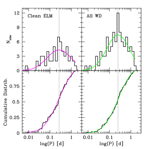
Figure 8: Period distribution of WD binaries in the clean ELM sample (left panels) and the full survey (right panels) with the best-fit lognormal distributions (solid lines). Vertical dotted lines mark the lognormal means, $P\simeq 0.25$ d.

4.3 Mass-Period Distribution: Link to Formation

According to binary evolution theory, ELM WDs can form from either a stable Roche lobe overflow channel or a common envelope channel (Li et al., 2019). The $P>1$ yr WD+MS binaries containing an ELM pre-WD (Vos et al., 2018) or ELM WD (Masuda et al., 2019; Jadhav et al., 2019) demonstrate that other evolutionary pathways also exist. For double WD binaries, the diagnostic parameters are ELM WD mass and orbital period, because mass and period should be tightly correlated in the Roche lobe overflow channel.

Following Li et al. (2019), we plot mass versus orbital period for our updated sample in Figure 9. Blue and red points are ELM WDs in the disk and halo, respectively. Green points are all the other WDs in the sample. The major uncertainty in this plot is systematic: objects with period aliases, which are drawn with open symbols at the best-fit period. As previously noted, disk and halo ELM WDs appear evenly mixed in parameter space. We draw dotted lines in Figure 9 as a guide to discussion.

The diagonal band of binaries at the bottom of Figure 9 is likely explained by the stable Roche lobe overflow channel. In the formation models, the ELM WD progenitors begin mass transfer near the end of the main sequence and produce ELM WD masses correlated with period extending up to $M=0.3$ $M_{\odot}$ (Li et al., 2019). The highest mass ELM WD we observe in this band is $M=0.24$ $M_{\odot}$.

Between about 0.22 $M_{\odot}$ and 0.32 $M_{\odot}$ there is a vertical band binaries seen only with $P<0.1$ d. This group of ELM WDs likely comes from the common envelope channel. In the formation models, the ELM WD progenitors begin mass transfer near the base of the red giant branch and produce more massive $M>0.21$ $M_{\odot}$ ELM WDs due to the energy required to eject the common envelope (Li et al., 2019). Interestingly, half (12/25) of the WDs in our sample with $P<0.1$ d are observed in this mass range. The median gravitational wave merger time of these binaries is $\tau=10^{8}$ yr.

Finally, we observe $M>0.3$ $M_{\odot}$ WDs with a diverse range of $P$. Our sample is not complete at these masses, but the observed period distribution appears consistent with the common envelope efficiency $\alpha_{\rm CE}=0.5$ binary population synthesis models of Li et al. (2019).

4.4 He+CO Merger Rate: Link to Outcomes

Once formed, ELM WD binary orbits shrink due to gravitational wave radiation. The gravitational wave merger timescale depends primarily on period,

$$\tau=47925\frac{(M_{1}+M_{2})^{1/3}}{M_{1}M_{2}}P^{8/3}~{}{\rm Myr}$$ (1)

where the masses are in $M_{\odot}$, the period $P$ is in days, and the time $\tau$ is in Myr (Kraft et al., 1962). For the clean ELM WD sample, $\tau$ ranges from 1 Myr (J0651+2844) to 700 Gyr (J1512+2615) and has a median value of $10$ Gyr.

Physically, ELM WDs are He-core WDs. Their unseen companions are typically 0.75 $M_{\odot}$ objects at 1.6 $R_{\odot}$ orbital separations – thus CO-core WDs – if the binaries have random inclination (Andrews et al., 2014; Boffin, 2015; Brown et al., 2016a).

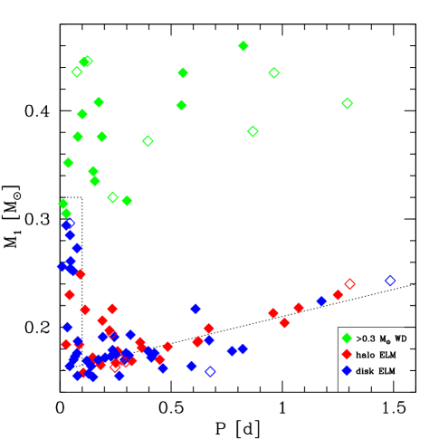
Figure 9: Mass of the visible WD versus binary period plotted on a linear scale. Blue and red points mark ELM WDs in the disk and halo, respectively. All other WDs with $>$0.3 $M_{\odot}$ are plotted in green. Binaries with period aliases are drawn with a single open symbol at their best-fit period. Dotted lines are drawn as a guide; the distribution suggests that ELM WDs form from both Roche lobe overflow and common envelope channels.

ELM WD binaries are thus He+CO WD binaries with typical mass ratios of about 1:4. A 1:4 mass ratio suggests that most binaries will evolve into stable helium mass-transfer systems, so-called AM CVn stars (Marsh et al., 2004). However, the dynamically driven double-degenerate double-detonation scenario posits that essentially all He+CO WD binaries have unstable mass transfer (Shen, 2015). We can test the outcome of He+CO WD mergers by comparing the merger rate against the formation rate of AM CVn.

We previously derived a merger rate for ELM WD binaries in the disk of the Milky Way using both reverse and forward-modeling approaches (Brown et al., 2016b). The rate calculation is dominated by the shortest-period binaries. The number of disk ELM WD binaries with $\tau<70$ Myr has grown by 33% (from 6 to 8) with the addition of J1043+0551 (Brown et al., 2017b) and J1738+2927 (this paper). However, we now exclude J0935+4411 (Kilic et al., 2014a) from the clean ELM WD sample because the WD is 0.32 $M_{\odot}$. The completeness correction has also changed because follow-up is now 97% complete in the clean ELM region. The updated merger rate for ELM WD binaries in the disk of the Milky Way is $2\times 10^{-3}$ yr^-1, 30% lower than the previous estimate but consistent within its factor of 2 uncertainty.

The 1:1 number ratio of binaries with $\tau<10$ Gyr and $\tau>10$ Gyr provides a complementary constraint. Binaries with $\tau>10$ Gyr accumulate over time. The only way to observe rapidly-merging systems without accumulating too many $\tau>10$ Gyr binaries is if the majority of ELM WD progenitors detach from the common envelope phase with $<$1 h orbital periods (Brown et al., 2016b).

The upshot is that the merger rate of observed ELM WD binaries exceeds the formation rate of stable mass-transfer AM CVn binaries in the Milky Way (Roelofs et al., 2007b; Carter et al., 2013) by a factor of at least 25. The total He+CO WD merger rate in the Galaxy can only be larger, because we do not observe all He+CO WDs. The ELM Survey observations thus require unstable mass transfer outcomes and support models in which most He+CO WDs merge (Shen, 2015).

4.5 Gravitational Wave Sources

WD binaries with $P<1$ h emit gravitational waves at mHz frequencies and are potentially multi-messenger sources detectable by the future LISA gravitational wave observatory. J0651+2844, for example, is an order of magnitude more luminous in gravitational waves (3 L_⊙) than in bolometric light (0.1 L_⊙).

Lamberts et al. (2019) recently combine binary population synthesis models with cosmological simulations of Milky Way-like galaxies to predict what type of binaries LISA will see (see also Korol et al., 2017; Breivik et al., 2019). He+CO WD binaries, like those observed here, are predicted to be 50% of the binaries individually resolved by LISA. The majority of sources should be in the disk, though the bulge and halo are also predicted to contribute detections.

To compare with the binaries we observe optically, Figure 10 plots the characteristic strain versus gravitational wave frequency $f=2/P$ for all 98 WD binaries. We also draw the 4 yr LISA sensitivity curve (solid line) (Robson et al., 2019) as a guide for discussion. Symbols and colors are the same as in Figure 9.

We compute characteristic strain using inclination,

$$h_{c}=3.4\times 10^{-23}\sqrt{\cos^{4}(i)+6\cos^{2}(i)+1}\mathcal{M}^{5/3}P^{-2/3}d^{-1},$$ (2)

where $\mathcal{M}=(M_{1}M_{2})^{3/5}(M_{1}+M_{2})^{-1/5}$ is the chirp mass in $M_{\odot}$, $P$ is in days, and $d$ is in kpc (Timpano et al., 2006; Roelofs et al., 2007a). We multiply by $\sqrt{(4~{}{\rm yr})f}$ to account for the S/N boost from the number of cycles during the LISA observation time (Robson et al., 2019). We note that most strain calculations implicitly assume $i=60\arcdeg$, which yields a strain systematically 1.6$\times$ too large for eclipsing binaries like J0651+2844. Ironically, non-velocity-variable ELM WDs may be among the highest strain systems since they (presumably) have low inclination, however we have no constraints on their orbital periods.

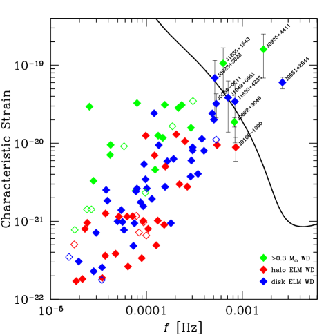
Figure 10: Characteristic strain $h_{c}$ times $\sqrt{(4~{}{\rm yr})f}$, the S/N boost from the number of cycles during the LISA observation time, versus gravitational wave frequency $f=2/P$ for all 98 WD binaries. Symbols are the same as Figure 9. Solid line is the LISA 4 yr sensitivity curve (Robson et al., 2019).

Our approach to Figure 10 is to compute strain 10,000 times per binary assuming random inclination and normally distributed measurement errors, including any inclination constraint. Four WD binaries in the ELM Survey are eclipsing (Steinfadt et al., 2010; Brown et al., 2011b, 2017b; Kilic et al., 2014a), eight have ellipsoidal variations (Kilic et al., 2011c; Hermes et al., 2012a, 2014; Bell et al., 2017), and 32 have X-ray and/or radio observations that rule out low inclination millisecond pulsar companions (Agüeros et al., 2009b, a; Kilic et al., 2011a, 2012, 2014b, 2016; Andrews et al., 2018). We also exclude inclinations that correspond to physically unlikely mass extremes: companions less massive than the observed ELM WD, or greater than 3 $M_{\odot}$. We detail the inclination constraints in the Appendix. Errorbars in Figure 10 are the 16% and 84% percentiles of the resulting strain distribution, and the values are listed in Table 3. For the sake of clarity, we label only those WD binaries near the 4 yr LISA sensitivity curve.

Interestingly, all six binaries on or above the 4 yr LISA sensitivity curve are disk objects, as predicted by the models. The strongest halo binary, J0822+3048, falls just below the sensitivity curve. However, the Lamberts et al. (2019) models do not match the observed distribution of periods. The model period distribution has a gap around $f=0.8$ mHz where most (4 of 7) of the observed binaries with periods below 1 h reside in our sample.

The highest S/N source J0651+2844. Because its spectroscopic distance is many times more accurate than its Gaia DR2 parallax, its characteristic strain in Figure 10 has a much smaller uncertainty than calculated by Kupfer et al. (2018). According to the LISA Detectability Calculator, J0651+2844 has a 4-yr S/N $\simeq 150$ (Q. S. Baghi, private communication). It would be very interesting to find more WD binaries like J0651+2844. Being a sample of one, however, implies that we may need to observe $\sim$100 more ELM WDs to find another J0651+2844.

A more productive approach to finding strong mHz gravitational wave sources may be to target bright and nearby ELM WD candidates. In the clean ELM WD sample, 10/62 (or 1-in-6) of the binaries have $P<0.05$ d (or $f>0.5$ mHz) where LISA is most sensitive. An untargeted approach, taken by the Zwicky Transient Factory, is to search for short-period eclipsing systems from all-sky time-series imaging (Burdge et al., 2019a, b).

5 Conclusions

The ELM Survey was a major observational program that targeted extremely low mass, He-core WDs on the basis of magnitude and color. It is now essentially complete within our color/magnitude selection limits in the SDSS footprint. One of the major goals of this paper is to consolidate all the measurements: 4,338 radial velocity measurements, 230 stellar atmosphere fits, 128 radial velocity orbital solutions, and 47 inclination constraints derived from follow-up optical, X-ray, and radio observations. New measurements include Chandra and GBT observations, plus stellar atmosphere fits and radial velocity solutions for 25 well-constrained new binaries.

We apply Gaia parallax and proper motion measurements to the sample for the first time, and find that ELM WD evolutionary tracks provide accurate luminosity estimates for candidates with $T_{\rm eff}>9,$500 K. However, most candidates with $<$9,000 K have radii and luminosities too large to be WDs on the basis of their parallax, and so are subdwarf A-type stars (a.k.a. field blue stragglers). This motivates us to define a clean set of WDs over which our observations are complete.

The ELM Survey contains a total of 98 WD+WD binaries, more than half of known detached double WD binaries in the Milky Way. In the clean sample, 35% of the binaries are halo objects on the basis of 3D space motions. Their orbital periods span $0.0089<P<1.5$ d and are correlated with He WD mass, providing evidence for both stable Roche lobe and unstable common envelope formation channels. We infer that most systems are He+CO WD binaries. The gravitational wave merger timescales imply a $2\times 10^{-3}$ yr^-1 merger rate of He+CO WD binaries in the disk of the Milky Way, which is a lower limit because we do not target all He+CO WD binaries. The merger rate is 25 times larger than the formation rate of stable mass transfer AM CVn binaries, thus our observations require unstable mass transfer outcomes for He+CO WD binary mergers (Shen, 2015; Brown et al., 2016b).

The observed binaries notably emit gravitational waves at mHz frequencies. Two ELM Survey discoveries, J0651+2844 and J0935+4411, will be detected at high S/N by the future LISA mission. Linking light and gravitational waves is important for making measurements beyond what either observational technique can achieve on its own. Tidal dissipation, for example, is expected to significantly influence WD temperature and rotation prior to mass transfer and merger (Fuller & Lai, 2014) and to appear as an accelerated $\dot{P}$ (Piro, 2011, 2019). Eclipse timing already provides exquisite $\dot{P}$ measurements for binaries like J0651+2844 (Hermes et al., 2012b, 2020), ZTF J1539+5027 (Burdge et al., 2019a), and PTF J0533+0209 (Burdge et al., 2019b), however optical constraints on mass are much less precise. LISA can provide an independent mass constraint for these systems, and, in conjunction with the optical $\dot{P}$, constrain the amount of tidal heating in merging pairs of WDs.

It would thus be very interesting to find more WD binaries that can serve as multi-messenger laboratories, systems we can observe with both light and gravity. To that end, we have begun the ELM Survey South (Kosakowski et al., 2020), targeting southern hemisphere ELM WD candidates using photometric surveys like VST Atlas (Shanks et al., 2015) and SkyMapper (Wolf et al., 2018). Gaia DR2 opens a new window on target selection using parallax, which works well at bright $G<18.5$ magnitudes (e.g. Pelisoli & Vos, 2019). Over the past year, we have also observed new ELM WD candidates using Gaia. Photometric surveys like the Zwicky Transient Facility, and the Large Synoptic Survey Telescope will help immensely as well (Korol et al., 2017). The future of ELM WD discoveries appears bright both in light and gravitational waves.

Appendix A WD Binary Inclination Constraints

Table A summarizes the inclination constraints for WD binaries in the ELM Survey, with links to the papers that published the measurements. The best inclination constraints come from time-series optical photometry (e.g. Hermes et al., 2014). Four eclipsing binaries (labeled Eclip.=1) have $i\simeq 90\arcdeg$ with $\sim$1$\arcdeg$ uncertainties. Ellipsoidal variation caused by tidal deformation of the WD also places an inclination constraint. Eight binaries with ellipsoidal variation (labeled E.V.=1) have $i=50-75\arcdeg$ with $\sim$10$\arcdeg$ uncertainties (Bell et al., 2018a). The absence of eclipses places another, weak, $i\lesssim 88\arcdeg$ constraint for WD binaries with well-measured optical light curves.

Radio and X-ray null detections place lower limits on inclination. As mentioned above, milli-second pulsars are commonly observed with low mass WD companions (Manchester et al., 2005; Panei et al., 2007). In all cases, however, ELM WD binaries with targeted Chandra (labeled X-ray=1) or Green Bank Telescope (labeled Radio=1) observations capable of detecting plausible pulsar companions find null detections. Null detections imply $M_{2}<1.4$ $M_{\odot}$. Solving the binary mass function for inclination,

$$i={\rm asin}\left(k\left(\frac{P}{2\pi G}\right)^{1/3}\frac{(M_{1}+M_{2})^{2/3}}{M_{2}}\right),$$ (A1)

an upper limit on $M_{2}$ places a lower limit on $i$ given the binary’s observed semi-amplitude $k$, period $P$, and derived mass $M_{1}$.

An optional inclination constraint, not listed in Table A, is the upper limit that comes from requiring $M_{2}>M_{1}$. Because the most massive star in a binary should evolve first, it is implausible for ELM WDs to have companions of lower mass. In practice, requiring $M_{2}>M_{1}$ provides only a weak inclination constraint; it affects the five ELM WD binaries in the clean sample with minimum $M_{2}$ less than the ELM WD mass (see Tables 2 and 3).

Table 4: ELM Survey WD Binary Inclination Constraints

Object	$i$	Eclip.	E.V.	X-ray	Radio	Reference
	(deg)
J0022$+$0031	$>21$	0	0	0	1	2
J0022$-$1014	$>18,<86.0$	0	0	0	1	2,9
J0056$-$0611	$>37,50^{+9}_{-7}$	0	1	0	1	0,9,6
J0106$-$1000	$56^{+11}_{-8}$	0	1	0	0	12,9,6
J0112$+$1835	$>45,66^{+10}_{-9}$	0	1	0	1	0,9,6
J0152$+$0749	$>43$	0	0	0	1	0
J0345$+$1748	$89.67\pm 0.12$	1	0	0	0	11
J0651$+$2844	$86.3\pm 1.0$	1	1	0	0	10
J0751$-$0141	$>60,85.4^{+4.2}_{-9.4}$	1	1	1	1	0,17
J0755$+$4800	$>52,<89.4$	0	0	1	1	0,18
J0802$-$0955	$>71$	0	0	0	1	3
J0811$+$0225	$>70,<88.4$	0	0	1	1	0,18
J0822$+$2753	$>52$	0	0	1	1	2,14
J0822$+$3048	$88.1^{+1.4}_{-2.3}$	1	0	0	0	8
J0825$+$1152	$<84.8$	0	0	0	0	9
J0849$+$0445	$>45,<85.7$	0	0	1	1	2,14,9
J0917$+$4638	$>29$	0	0	1	1	1
J0923$+$3028	$<84.6$	0	0	0	0	9
J0935$+$4411	$<70$	0	0	0	0	16
J1005$+$0542	$>35$	0	0	0	1	0
J1043$+$0551	$<85.7$	0	0	0	0	7
J1053$+$5200	$>26,<82.0$	0	0	0	1	2,9
J1054$-$2121	$72^{+9}_{-10}$	0	1	0	0	4,6
J1056$+$6536	$>25,<84.9$	0	0	0	1	2,9
J1104$+$0918	$>35$	0	0	0	1	0
J1108$+$1512	$<87.2$	0	0	0	0	4
J1141$+$3850	$>49$	0	0	0	1	0
J1151$+$5858	$>46$	0	0	0	1	0
J1233$+$1602	$>54,<90.0$	0	0	0	1	0,9
J1234$-$0228	$>13,<71.5$	0	0	0	1	2,9
J1238$+$1946	$>48$	0	0	0	1	0
J1436$+$5010	$>36,<84.4$	0	0	0	1	2,9
J1443$+$1509	$>55,<88.3$	0	0	1	1	0,18
J1449$+$1717	$<87.6$	0	0	0	0	4
J1518$+$0658	$>43$	0	0	0	1	0
J1538$+$0252	$>42$	0	0	0	1	0
J1618$+$3854	$<88.1$	0	0	0	0	5
J1625$+$3632	$>10$	0	0	0	1	2
J1630$+$4233	$>24,<82.8$	0	0	0	1	2,13
J1738$+$2927	$<85.8$	0	0	0	0	0
J1741$+$6526	$>64,75^{+7}_{-8}$	0	1	1	1	0,9,17,6
J1840$+$6423	$>52$	0	0	0	1	0
J2103$-$0027	$>48$	0	0	0	1	0
J2119$-$0018	$68^{+10}_{-11}$	0	1	0	0	9
J2132$+$0754	$>58,<87.5$	0	0	1	1	0,18
J2236$+$2232	$>34$	0	0	1	1	15
J2338$-$2052	$<83.8$	0	0	0	0	9

References. — (0) this paper, (1) Agüeros et al. (2009b), (2) Agüeros et al. (2009a), (3) Andrews et al. (2018), (4) Bell et al. (2017), (5) Bell et al. (2018b), (6) Bell et al. (2018a), (7) Brown et al. (2017a), (8) Brown et al. (2017b), (9) Hermes et al. (2014), (10) Hermes et al. (2020), (11) Kaplan et al. (2014), (12) Kilic et al. (2011c), (13) Kilic et al. (2011b), (14) Kilic et al. (2012), (15) Kilic et al. (2013), (16) Kilic et al. (2014a), (17) Kilic et al. (2014b), (18) Kilic et al. (2017)

References

- Agüeros et al. (2009a) Agüeros, M. A., Camilo, F., Silvestri, N. M., et al. 2009a, ApJ, 697, 283
- Agüeros et al. (2009b) Agüeros, M. A., Heinke, C., Camilo, F., et al. 2009b, ApJ, 700, L123
- Alam et al. (2015) Alam, S., Albareti, F. D., Allende Prieto, C., et al. 2015, ApJS, 219, 12
- Althaus et al. (2013) Althaus, L. G., Miller Bertolami, M. M., & Córsico, A. H. 2013, A&A, 557, A19
- Amaro-Seoane et al. (2017) Amaro-Seoane, P., Audley, H., Babak, S., et al. 2017, arXiv e-prints, arXiv:1702.00786
- Andrews et al. (2018) Andrews, J. J., Agüeros, M. A., Camilo, F., et al. 2018, Research Notes of the AAS, 2, 60
- Andrews et al. (2014) Andrews, J. J., Price-Whelan, A. M., & Agüeros, M. A. 2014, ApJ, 797, L32
- Antoniadis et al. (2013) Antoniadis, J., Freire, P. C. C., Wex, N., et al. 2013, Science, 340, 448
- Badenes et al. (2009) Badenes, C., Mullally, F., Thompson, S. E., & Lupton, R. H. 2009, ApJ, 707, 971
- Bell et al. (2017) Bell, K. J., Gianninas, A., Hermes, J. J., et al. 2017, ApJ, 835, 180
- Bell et al. (2018a) Bell, K. J., Hermes, J. J., & Kuszlewicz, J. S. 2018a, in 21st European Workshop on White Dwarfs, ed. B. Castanheira, F. Campos, & M. Montgomery, EuroWD (Austin: Texas ScholarWorks)
- Bell et al. (2018b) Bell, K. J., Pelisoli, I., Kepler, S. O., et al. 2018b, A&A, 617, A6
- Beloborodov (2002) Beloborodov, A. M. 2002, ApJ, 566, L85
- Boffin (2015) Boffin, H. M. J. 2015, A&A, 575, L13
- Bogdanov et al. (2006) Bogdanov, S., Grindlay, J. E., Heinke, C. O., et al. 2006, ApJ, 646, 1104
- Bond & MacConnell (1971) Bond, H. E. & MacConnell, D. J. 1971, ApJ, 165, 51
- Breivik et al. (2019) Breivik, K., Coughlin, S. C., Zevin, M., et al. 2019, ApJ, submitted
- Brown et al. (2011a) Brown, J. M., Kilic, M., Brown, W. R., & Kenyon, S. J. 2011a, ApJ, 729, 2
- Brown et al. (2012a) Brown, W. R., Geller, M. J., & Kenyon, S. J. 2012a, ApJ, 751, 55
- Brown et al. (2006) Brown, W. R., Geller, M. J., Kenyon, S. J., & Kurtz, M. J. 2006, ApJ, 647, 303
- Brown et al. (2016a) Brown, W. R., Gianninas, A., Kilic, M., Kenyon, S. J., & Allende Prieto, C. 2016a, ApJ, 818, 155
- Brown et al. (2010) Brown, W. R., Kilic, M., Allende Prieto, C., & Kenyon, S. J. 2010, ApJ, 723, 1072
- Brown et al. (2012b) —. 2012b, ApJ, 744, 142
- Brown et al. (2017a) Brown, W. R., Kilic, M., & Gianninas, A. 2017a, ApJ, 839, 23
- Brown et al. (2011b) Brown, W. R., Kilic, M., Hermes, J. J., et al. 2011b, ApJ, 737, L23
- Brown et al. (2016b) Brown, W. R., Kilic, M., Kenyon, S. J., & Gianninas, A. 2016b, ApJ, 824, 46
- Brown et al. (2017b) Brown, W. R., Kilic, M., Kosakowski, A., & Gianninas, A. 2017b, ApJ, 847, 10
- Burdge et al. (2019a) Burdge, K. B., Coughlin, M. W., Fuller, J., et al. 2019a, Nature, 571, 528
- Burdge et al. (2019b) Burdge, K. B., Fuller, J., Phinney, E. S., et al. 2019b, ApJ, 886, L12
- Carter et al. (2013) Carter, P. J., Marsh, T. R., Steeghs, D., et al. 2013, MNRAS, 429, 2143
- Cash (1976) Cash, W. 1976, A&A, 52, 307
- Chiba & Beers (2000) Chiba, M. & Beers, T. C. 2000, AJ, 119, 2843
- Clemens et al. (2004) Clemens, J. C., Crain, J. A., & Anderson, R. 2004, in Proc. SPIE, ed. A. F. M. Moorwood & M. Iye, Vol. 5492, 331–340
- Cordes & Lazio (2002) Cordes, J. M. & Lazio, T. J. W. 2002, arXiv, 0207156
- Dickey & Lockman (1990) Dickey, J. M. & Lockman, F. J. 1990, ARA&A, 28, 215
- Eggleton (1983) Eggleton, P. P. 1983, ApJ, 268, 368
- Eisenstein et al. (2006) Eisenstein, D. J., Liebert, J., Harris, H. C., et al. 2006, ApJS, 167, 40
- Fabricant et al. (1998) Fabricant, D., Cheimets, P., Caldwell, N., & Geary, J. 1998, PASP, 110, 79
- Forestell et al. (2014) Forestell, L. M., Heinke, C. O., Cohn, H. N., et al. 2014, MNRAS, 441, 757
- Fruscione et al. (2006) Fruscione, A., McDowell, J. C., Allen, G. E., et al. 2006, in SPIE Conference Series, Vol. 6270, Proc. SPIE, ed. Silva, D. R. and Doxsey, R. E. (SPIE), 62701V
- Fuller & Lai (2014) Fuller, J. & Lai, D. 2014, MNRAS, 444, 3488
- Geier et al. (2011) Geier, S., Maxted, P. F. L., Napiwotzki, R., et al. 2011, A&A, 526, A39
- Gianninas et al. (2011) Gianninas, A., Bergeron, P., & Ruiz, M. T. 2011, ApJ, 743, 138
- Gianninas et al. (2014) Gianninas, A., Dufour, P., Kilic, M., et al. 2014, ApJ, 794, 35
- Gianninas et al. (2015) Gianninas, A., Kilic, M., Brown, W. R., Canton, P., & Kenyon, S. J. 2015, ApJ, 812, 167
- Han (1998) Han, Z. 1998, MNRAS, 296, 1019
- Heber (2009) Heber, U. 2009, ARA&A, 47, 211
- Heinke et al. (2006) Heinke, C. O., Rybicki, G. B., Narayan, R., & Grindlay, J. E. 2006, ApJ, 644, 1090
- Hermes et al. (2020) Hermes, J. J., Brown, W. R., Bell, K. J., et al. 2020, in prep.
- Hermes et al. (2014) Hermes, J. J., Brown, W. R., Kilic, M., et al. 2014, ApJ, 792, 39
- Hermes et al. (2012a) Hermes, J. J., Kilic, M., Brown, W. R., Montgomery, M. H., & Winget, D. E. 2012a, ApJ, 749, 42
- Hermes et al. (2012b) Hermes, J. J., Kilic, M., Brown, W. R., et al. 2012b, ApJ, 757, L21
- Hook et al. (2004) Hook, I. M., Jørgensen, I., Allington-Smith, J. R., et al. 2004, PASP, 116, 425
- Iben (1990) Iben, Jr., I. 1990, ApJ, 353, 215
- Iben et al. (1997) Iben, Icko, J., Tutukov, A. V., & Yungelson, L. R. 1997, ApJ, 475, 291
- Istrate et al. (2016) Istrate, A. G., Marchant, P., Tauris, T. M., et al. 2016, A&A, 595, A35
- Jadhav et al. (2019) Jadhav, V. V., Sindhu, N., & Subramaniam, A. 2019, ApJ, 886, 13
- Kaplan et al. (2014) Kaplan, D. L., Marsh, T. R., Walker, A. N., et al. 2014, ApJ, 780, 167
- Kargaltsev et al. (2012) Kargaltsev, O., Durant, M., Pavlov, G. G., & Garmire, G. 2012, ApJS, 201, 37
- Kenyon & Garcia (1986) Kenyon, S. J. & Garcia, M. R. 1986, AJ, 91, 125
- Kepler et al. (2015) Kepler, S. O., Pelisoli, I., Koester, D., et al. 2015, MNRAS, 446, 4078
- Kepler et al. (2016) —. 2016, MNRAS, 455, 3413
- Kilic et al. (2007) Kilic, M., Allende Prieto, C., Brown, W. R., & Koester, D. 2007, ApJ, 660, 1451
- Kilic et al. (2010) Kilic, M., Brown, W. R., Allende Prieto, C., Kenyon, S. J., & Panei, J. A. 2010, ApJ, 716, 122
- Kilic et al. (2011a) Kilic, M., Brown, W. R., Allende Prieto, C., et al. 2011a, ApJ, 727, 3
- Kilic et al. (2012) —. 2012, ApJ, 751, 141
- Kilic et al. (2014a) Kilic, M., Brown, W. R., Gianninas, A., et al. 2014a, MNRAS, 444, L1
- Kilic et al. (2017) —. 2017, MNRAS, 471, 4218
- Kilic et al. (2016) Kilic, M., Brown, W. R., Heinke, C. O., et al. 2016, MNRAS, 460, 4176
- Kilic et al. (2011b) Kilic, M., Brown, W. R., Hermes, J. J., et al. 2011b, MNRAS, 418, L157
- Kilic et al. (2011c) Kilic, M., Brown, W. R., Kenyon, S. J., et al. 2011c, MNRAS, 413, L101
- Kilic et al. (2013) Kilic, M., Gianninas, A., Brown, W. R., et al. 2013, MNRAS, 434, 3582
- Kilic et al. (2014b) Kilic, M., Hermes, J. J., Gianninas, A., et al. 2014b, MNRAS, 438, L26
- Kilkenny et al. (1997) Kilkenny, D., O’Donoghue, D., Koen, C., Stobie, R. S., & Chen, A. 1997, MNRAS, 287, 867
- Kleinman et al. (2013) Kleinman, S. J., Kepler, S. O., Koester, D., et al. 2013, ApJS, 204, 5
- Korol et al. (2017) Korol, V., Rossi, E. M., Groot, P. J., et al. 2017, MNRAS, 470, 1894
- Kosakowski et al. (2020) Kosakowski, A., Kilic, M., Brown, W. R., et al. 2020, submitted
- Kraft et al. (1962) Kraft, R. P., Mathews, J., & Greenstein, J. L. 1962, ApJ, 136, 312
- Kupfer et al. (2018) Kupfer, T., Korol, V., Shah, S., et al. 2018, MNRAS, 480, 302
- Kurtz & Mink (1998) Kurtz, M. J. & Mink, D. J. 1998, PASP, 110, 934
- Lamberts et al. (2019) Lamberts, A., Blunt, S., Littenberg, T., et al. 2019, MNRAS, 490, 5888
- Li et al. (2019) Li, Z., Chen, X., Chen, H.-L., & Han, Z. 2019, ApJ, 871, 148
- Lindegren et al. (2018) Lindegren, L., Hernandez, J., Bombrun, A., et al. 2018, A&A, 616, A2
- Luo et al. (2015) Luo, A. L., Zhao, Y.-H., Zhao, G., et al. 2015, Research in Astronomy and Astrophysics, 15, 1095
- Lyne & Manchester (1988) Lyne, A. G. & Manchester, R. N. 1988, MNRAS, 234, 477
- Manchester et al. (2005) Manchester, R. N., Hobbs, G. B., Teoh, A., & Hobbs, M. 2005, AJ, 129, 1993
- Marigo et al. (2017) Marigo, P., Girardi, L., Bressan, A., et al. 2017, ApJ, 835, 77
- Marsh (2019) Marsh, T. R. 2019, Close Double White Dwarfs in Gaia
- Marsh et al. (1995) Marsh, T. R., Dhillon, V. S., & Duck, S. R. 1995, MNRAS, 275, 828
- Marsh et al. (2004) Marsh, T. R., Nelemans, G., & Steeghs, D. 2004, MNRAS, 350, 113
- Martini et al. (2014) Martini, P., Elias, J., Points, S., et al. 2014, in Proc. SPIE, ed. Ramsay, S. K and McLean, I. S. and Takami, H., Vol. 9147 (Montreal, Canada: SPIE), 91470Z
- Masuda et al. (2019) Masuda, K., Kawahara, H., Latham, D. W., et al. 2019, ApJ, 881, L3
- McCook & Sion (1987) McCook, G. P. & Sion, E. M. 1987, ApJS, 65, 603
- Moe & Di Stefano (2017) Moe, M. & Di Stefano, R. 2017, ApJS, 230, 15
- Napiwotzki et al. (2019) Napiwotzki, R., Karl, C. A., Lisker, T., et al. 2019, A&A, accepted
- Nebot Gómez-Morán et al. (2011) Nebot Gómez-Morán, A., Gänsicke, B. T., Schreiber, M. R., et al. 2011, A&A, 536, A43
- Nelemans et al. (2001) Nelemans, G., Yungelson, L. R., Portegies Zwart, S. F., & Verbunt, F. 2001, A&A, 365, 491
- Panei et al. (2007) Panei, J. A., Althaus, L. G., Chen, X., & Han, Z. 2007, MNRAS, 382, 779
- Pelisoli et al. (2019) Pelisoli, I., Bell, K. J., Kepler, S. O., & Koester, D. 2019, MNRAS, 482, 3831
- Pelisoli et al. (2018a) Pelisoli, I., Kepler, S. O., & Koester, D. 2018a, MNRAS, 475, 2480
- Pelisoli et al. (2018b) Pelisoli, I., Kepler, S. O., Koester, D., Castanheira, B. G., Romero, A. D., & Fraga, L. 2018b, MNRAS, 478, 867
- Pelisoli et al. (2017) Pelisoli, I., Kepler, S. O., Koester, D., & Romero, A. D. 2017, in ASP Conf. Ser.: 20th European Workshop on White Dwarfs, ed. P.-E. Tremblay, B. Gaensicke, & T. Marsh, Vol. 509 (San Francisco: ASP), 447
- Pelisoli & Vos (2019) Pelisoli, I. & Vos, J. 2019, MNRAS, 488, 2892
- Piro (2011) Piro, A. L. 2011, ApJ, 740, L53
- Piro (2019) —. 2019, ApJ, 885, L2
- Press et al. (1992) Press, W. H., Teukolsky, S. A., Vetterling, W. T., & Flannery, B. P. 1992, Numerical recipes in C. The art of scientific computing (Cambridge: University Press, 2nd ed.)
- Preston & Sneden (2000) Preston, G. W. & Sneden, C. 2000, AJ, 120, 1014
- Raddi et al. (2017) Raddi, R., Gentile Fusillo, N. P., Pala, A. F., et al. 2017, MNRAS, 472, 4173
- Ransom et al. (2003) Ransom, S. M., Cordes, J. M., & Eikenberry, S. S. 2003, ApJ, 589, 911
- Ransom et al. (2002) Ransom, S. M., Eikenberry, S. S., & Middleditch, J. 2002, AJ, 124, 1788
- Rebassa-Mansergas et al. (2007) Rebassa-Mansergas, A., Gänsicke, B. T., Rodríguez-Gil, P., Schreiber, M. R., & Koester, D. 2007, MNRAS, 382, 1377
- Rebassa-Mansergas et al. (2010) Rebassa-Mansergas, A., Gänsicke, B. T., Schreiber, M. R., Koester, D., & Rodríguez-Gil, P. 2010, MNRAS, 402, 620
- Rebassa-Mansergas et al. (2012) Rebassa-Mansergas, A., Nebot Gómez-Morán, A., Schreiber, M. R., et al. 2012, MNRAS, 419, 806
- Reid et al. (2009) Reid, M. J., Menten, K. M., Zheng, X. W., et al. 2009, ApJ, 700, 137
- Robson et al. (2019) Robson, T., Cornish, N. J., & Liu, C. 2019, Classical and Quantum Gravity, 36, 105011
- Roelofs et al. (2007a) Roelofs, G. H. A., Groot, P. J., Benedict, G. F., et al. 2007a, ApJ, 666, 1174
- Roelofs et al. (2007b) Roelofs, G. H. A., Nelemans, G., & Groot, P. J. 2007b, MNRAS, 382, 685
- Schmidt et al. (1989) Schmidt, G. D., Weymann, R. J., & Foltz, C. B. 1989, PASP, 101, 713
- Scholz & Stephens (1987) Scholz, F. W. & Stephens, M. A. 1987, Journal of the American Statistical Association, 82, 918
- Schönrich et al. (2010) Schönrich, R., Binney, J., & Dehnen, W. 2010, MNRAS, 403, 1829
- Shanks et al. (2015) Shanks, T., Metcalfe, N., Chehade, B., et al. 2015, MNRAS, 451, 4238
- Shen (2015) Shen, K. J. 2015, ApJ, 805, L6
- Shporer et al. (2010) Shporer, A., Kaplan, D. L., Steinfadt, J. D. R., et al. 2010, ApJ, 725, L200
- Steinfadt et al. (2010) Steinfadt, J. D. R., Kaplan, D. L., Shporer, A., Bildsten, L., & Howell, S. B. 2010, ApJ, 716, L146
- Strom (1969) Strom, S. E. 1969, in Theory and Observation of Normal Stellar Atmospheres, ed. O. Gingerich (Cambridge: MIT), 99
- Tian et al. (2017) Tian, H.-J., Gupta, P., Sesar, B., et al. 2017, ApJS, 232, 4
- Timpano et al. (2006) Timpano, S. E., Rubbo, L. J., & Cornish, N. J. 2006, Phys. Rev. D, 73, 122001
- Tody (1986) Tody, D. 1986, in Proc. SPIE, Vol. 627, Instrumentation in astronomy VI, ed. D. L. Crawford (Bellingham, WA:SPIE), 733
- Tody (1993) Tody, D. 1993, in ASP Conf. Ser. Vol. 52, Astronomical Data Analysis Software and Systems II, ed. R. J. Hanisch, R. J. V. Brissenden, & J. Barnes (San Francisco: ASP), 173
- Tremblay & Bergeron (2009) Tremblay, P.-E. & Bergeron, P. 2009, ApJ, 696, 1755
- Tremblay et al. (2011) Tremblay, P. E., Bergeron, P., & Gianninas, A. 2011, ApJ, 730, 128
- Tremblay et al. (2015) Tremblay, P.-E., Gianninas, A., Kilic, M., et al. 2015, ApJ, 809, 148
- van Kerkwijk et al. (2005) van Kerkwijk, M. H., Bassa, C. G., Jacoby, B. A., & Jonker, P. G. 2005, in ASP Conf. Ser. Vol. 328, Binary Radio Pulsars, ed. F. A. Rasio & I. H. Stairs (San Francisco: ASP), 357
- van Kerkwijk et al. (1996) van Kerkwijk, M. H., Bergeron, P., & Kulkarni, S. R. 1996, ApJ, 467, L89
- van Leeuwen et al. (2007) van Leeuwen, J., Ferdman, R. D., Meyer, S., & Stairs, I. 2007, MNRAS, 374, 1437
- Vos et al. (2018) Vos, J., Zorotovic, M., Vučković, M., Schreiber, M. R., & Østensen, R. 2018, MNRAS, 477, L40
- Webbink (1984) Webbink, R. F. 1984, ApJ, 277, 355
- Weisskopf et al. (2002) Weisskopf, M. C., Brinkman, B., Canizares, C., et al. 2002, PASP, 114, 1
- Wolf et al. (2018) Wolf, C., Onken, C. A., Luvaul, L. C., et al. 2018, PASA, 35, e010
- Yu et al. (2019) Yu, J., Li, Z., Zhu, C., et al. 2019, ApJ, 885, 20
- Zorotovic et al. (2010) Zorotovic, M., Schreiber, M. R., Gänsicke, B. T., & Nebot Gómez-Morán, A. 2010, A&A, 520, A86