Theory inspired deep network for instantaneous-frequency extraction and signal components recovery from discrete blind-source data

Charles K. Chui, Ningning Han and H. N. Mhaskar Department of Mathematics, Hong Kong Baptist University. This author is also associated with Department of Statistics, Stanford University, CA 94305, U.S.A. email: ckchui@stanford.edu. He is a Life Fellow of IEEE and his research is partially supported by the Hong Kong Research Council, under Projects \sharp 12300917 and \sharp 12303218, and HKBU Grants \sharp RC-ICRS/16-17/03 and \sharp RC-FNRA-IG/18-19/SCI/01. Department of Mathematics, Hong Kong Baptist University, Hong Kong. email: ningninghan@hkbu.edu.hk. His research is supported by the Hong Kong Research Council, under Projects \sharp 12300917 and \sharp 12303218.Institute of Mathematical Sciences, Claremont Graduate University, Claremont, CA 91711, U.S.A. email: hrushikesh.mhaskar@cgu.edu
Abstract

This paper is concerned with the inverse problem of recovering the unknown signal components, along with extraction of their instantaneous frequencies (IFs), governed by the adaptive harmonic model (AHM), from discrete (and possibly non-uniform) samples of the blind-source composite signal. None of the existing decomposition methods and algorithms, including the most popular empirical mode decomposition (EMD) computational scheme and its current modifications, is capable of solving this inverse problem. In order to meet the AHM formulation and to extract the IFs of the decomposed components, called intrinsic mode functions (IMFs), each IMF of EMD is extended to an analytic function in the upper half of the complex plane via the Hilbert transform, followed by taking the real part of the polar form of the analytic extension. Unfortunately, this approach most often fails to resolve the inverse problem satisfactorily. More recently, to resolve the inverse problem, the notion of synchrosqueezed wavelet transform (SST) was proposed by Daubechies and Maes, and further developed in many other papers, while a more direct method, called signal separation operation (SSO), was proposed and developed in our previous work published in the journal, Applied and Computational Harmonic Analysis, vol. 30(2):243-261, 2016. In the present paper, we propose a synthesis of SSO using a deep neural network, based directly on a discrete sample set, that may be non-uniformly sampled, of the blind-source signal. Our method is localized, as illustrated by a number of numerical examples, including components with different signal arrival and departure times. It also yields short-term prediction of the signal components, along with their IFs. Our neural networks are inspired by theory, designed so that they do not require any training in the traditional sense.

Keywords: Separation of components, non-stationary signals, deep networks, super-resolution.

1 Introduction and Results

Many problems that arise from sensor arrays, stochastic control, mobile communication, and signal processing in general, are modeled by a linear combination of damped sinusoids, with stationary frequencies. However, in the current age of big data, particularly in time series analysis, the sinusoids are mostly non-stationary, in that the phase functions are not necessarily linear in time. A general mathematical model for such non-stationary signals or time series may be formulated by

j=1KAj(t)cosϕj(t)+A0(t),superscriptsubscript𝑗1𝐾subscript𝐴𝑗𝑡subscriptitalic-ϕ𝑗𝑡subscript𝐴0𝑡\sum_{j=1}^{K}A_{j}(t)\cos\phi_{j}(t)+A_{0}(t), (1.1)

or more generally by the complex variant

fI(t)=j=1KAj(t)exp(iϕj(t))+A0(t),subscript𝑓𝐼𝑡superscriptsubscript𝑗1𝐾subscript𝐴𝑗𝑡𝑖subscriptitalic-ϕ𝑗𝑡subscript𝐴0𝑡f_{I}(t)=\sum_{j=1}^{K}A_{j}(t)\exp(i\phi_{j}(t))+A_{0}(t), (1.2)

where the phase functions ϕj(t)subscriptitalic-ϕ𝑗𝑡\phi_{j}(t) are differentiable, the amplitude functions Aj(t)subscript𝐴𝑗𝑡A_{j}(t) are complex-valued and continuous, and A0(t)subscript𝐴0𝑡A_{0}(t) is a minimally oscillatory real-valued function, called the trend of fI(t)subscript𝑓𝐼𝑡f_{I}(t). Here, the subscript I𝐼I of fI(t)subscript𝑓𝐼𝑡f_{I}(t) is used to indicate that noise is not attached to the model. This is only a convenience of notation. Our methods do work well in the presence of noise, as will be proved theoretically in Theorem 2.1 and experimentally in Section 5. Without the trend function A0(t)subscript𝐴0𝑡A_{0}(t) in (1.1), the model is called the amplitude modulation-frequency modulation (AM-FM) model in signal processing, and the adaptive harmonic model (AHM) in the current mathematics literature (see, for example, [17, 9, 19, 6, 8, 5]). In our recent paper [7], the model (1.2) was called the Hilbert spectrum model (HSM). The objective of this paper is to introduce and develop an efficient and effective construction of deep networks for solving the inverse problem of recovering the number K𝐾K of terms in (1.2), the instantaneous frequencies (IFs) defined by ϕj(t)subscriptsuperscriptitalic-ϕ𝑗𝑡\phi^{\prime}_{j}(t), the amplitude functions Aj(t)subscript𝐴𝑗𝑡A_{j}(t), and the signal components fj(t):=Aj(t)cosϕj(t)assignsubscript𝑓𝑗𝑡subscript𝐴𝑗𝑡subscriptitalic-ϕ𝑗𝑡f_{j}(t):=A_{j}(t)\cos\phi_{j}(t), for j=1,,K𝑗1𝐾j=1,\cdots,K, as well as the trend A0(t)subscript𝐴0𝑡A_{0}(t), from a sufficiently “dense” finite data set fI(tk):k=0,,N:subscript𝑓𝐼subscript𝑡𝑘𝑘0𝑁f_{I}(t_{k}):k=0,\cdots,N, that are allowed to be non-uniformly sampled on a bounded time interval [b,c]𝑏𝑐[b,c]. Of course our constructions and theoretical development apply to infinite non-uniform data samples on an infinite interval as well, simply by ignoring the need of meeting the requirement of certain boundary conditions.

It is important to point out that our objective of solving an inverse problem is different from that of the popular empirical mode decomposition (EMD) method, introduced in [14]. Indeed, EMD is an ad hoc computational scheme for the decomposition of a non-stationary signal or time series g(t)𝑔𝑡g(t) into its intrinsic mode functions “IMFs” with residue, called the “trend”, without the concern of recovering the actual IMFs and trend that constitute the source signal or time series g(t)𝑔𝑡g(t). To emphasize the difference between EMD and our inverse problem, we recall the pioneering work [13] of Gaspard de Prony in resolving an exponential sum H(t)𝐻𝑡H(t) with K𝐾K exponents and K𝐾K corresponding constant coefficients, from 2K2𝐾2K samples H(0),H(1),,H(2K1)𝐻0𝐻1𝐻2𝐾1H(0),H(1),\cdots,H(2K-1), where K𝐾K is known, by first computing the K𝐾K exponents before computing the K𝐾K coefficients. In particular, if the exponents are eitωjsuperscript𝑒𝑖𝑡subscript𝜔𝑗e^{it\omega_{j}}, with ω1<ω2<<ωKsubscript𝜔1subscript𝜔2subscript𝜔𝐾\omega_{1}<\omega_{2}<\cdots<\omega_{K}, Prony’s method can be applied to solving the inverse problem (1.2), at least in theory, for stationary signals without the trend A0(t)subscript𝐴0𝑡A_{0}(t). Unfortunately, Prony’s method fails when some of the frequencies ωjsubscript𝜔𝑗\omega_{j} are very close to one another. The reason is that when these unknown exponents are considered as zeros of a polynomial p(z)𝑝𝑧p(z), with coefficients to be computed from Hankel matrix inversion, computation of these coefficients and the zeros from solving some corresponding eigenvalue problem is highly unstable. In any case, the procedure of first recovering the instantaneous frequencies before computing the signal components, as pioneered by Daubechies in [10, 9], and just about all later development in mathematics, including [17, 20, 5, 6, 19, 8, 7], is opposite to that of EMD, which first computes the signal components, called intrinsic mode functions (IMFs) by repeated applications of the “sifting process”, before computing the instantaneous frequencies by applying the Hilbert transform to each IMF.

On the other hand, the approach in our present paper is substantially different from those in the published literature, including [19, 17, 10, 9, 20, 5, 6, 8, 7]. First, unlike these papers, we work with non-uniform samples of fIsubscript𝑓𝐼f_{I}. We then approximate fIsubscript𝑓𝐼f_{I} using a spline quasi-interpolant [1]. This quasi-interpolant can be implemented using deep networks as suggested in [15]. The signal separation operator, (SSO), proposed in [6] can then be evaluated using uniform samples of this quasi-interpolant. The SSO operator evaluates a trigonometric polynomial, which can also be synthesized using a further neural network as proved in [16], and its thresholding by another layer of a network computing the rectified linear units ReLU activation functions. As in [6], clustering and finding local maxima then lead to the determination of the instantaneous frequencies. Importantly, in contrast to [9], we obtain the (complex) amplitudes simply by evaluating the SSO at these frequencies.

One interesting aspect of our construction is that the deep networks need not be “trained” in the usual sense, but are theory inspired, in that their parameters are prescribed by the theory without training. Our constructions are presented schematically in Figure 1 below.

Refer to caption
Figure 1: Theory inspired deep network to compute the thresholded values of SSO given non-uniform samples of the signal fIsubscript𝑓𝐼f_{I}.

After describing our Signal Separation Operator defined in [6] in Section 2, we develop the spline approximation in Section 3. The actual construction of deep networks as in Figure 1 is described in detail in Section 4, and illustrated in Section 5.

2 Signal separation operator

In this section, we review our construction of the signal separation operator (SSO) and its properties in [6]. In [6], trend extraction was done separately; the operator SSO is designed to separate from the Hilbert spectrum model

f(t)=j=1Kfj(t),fj(t)=Aj(t)exp(iϕj(t)),j=1,,K,formulae-sequence𝑓𝑡superscriptsubscript𝑗1𝐾subscript𝑓𝑗𝑡formulae-sequencesubscript𝑓𝑗𝑡subscript𝐴𝑗𝑡𝑖subscriptitalic-ϕ𝑗𝑡𝑗1𝐾f(t)=\sum_{j=1}^{K}f_{j}(t),\qquad f_{j}(t)=A_{j}(t)\exp(i\phi_{j}(t)),\quad j=1,\cdots,K, (2.1)

the components fk(t)subscript𝑓𝑘𝑡f_{k}(t) and the instantaneous frequencies ϕk(t)superscriptsubscriptitalic-ϕ𝑘𝑡\phi_{k}^{\prime}(t), finding the number K𝐾K of these quantities in the process.

The following definition summarizes the conditions assumed on the signal.

Definition 2.1.

For each t𝑡t\in{\mathbb{R}}, let (t)𝑡\mathcal{H}(t) denote the collection of functions f𝑓f of the form (2.1) where each component fj(t)=Aj(t)exp(iϕj(t))subscript𝑓𝑗𝑡subscript𝐴𝑗𝑡𝑖subscriptitalic-ϕ𝑗𝑡f_{j}(t)=A_{j}(t)\exp(i\phi_{j}(t)), j=1,,K𝑗1𝐾j=1,\cdots,K, satisfies each of the following conditions.

  1. 1.

    Aj::subscript𝐴𝑗A_{j}:{\mathbb{R}}\to{\mathbb{C}} is continuous, and ϕj::subscriptitalic-ϕ𝑗\phi_{j}:{\mathbb{R}}\to{\mathbb{R}} is continuously differentiable.

  2. 2.

    With

    B=B(t):=max1jK|ϕj(t)|,𝐵𝐵𝑡assignsubscript1𝑗𝐾superscriptsubscriptitalic-ϕ𝑗𝑡B=B(t):=\max_{1\leq j\leq K}|\phi_{j}^{\prime}(t)|, (2.2)

    there exists α=α(t)>0𝛼𝛼𝑡0\alpha=\alpha(t)>0 with the following property: For any u𝑢u with |u|α1(8πB)1/2𝑢superscript𝛼1superscript8𝜋𝐵12|u|\leq\alpha^{-1}(8\pi B)^{-1/2}, and j=1,,K𝑗1𝐾j=1,\cdots,K,

    |Aj(t+u)Aj(t)|α3|u||Aj(t)|,|ϕj(t+u)ϕj(t)|α3|u||ϕj(t)|.formulae-sequencesubscript𝐴𝑗𝑡𝑢subscript𝐴𝑗𝑡superscript𝛼3𝑢subscript𝐴𝑗𝑡superscriptsubscriptitalic-ϕ𝑗𝑡𝑢superscriptsubscriptitalic-ϕ𝑗𝑡superscript𝛼3𝑢superscriptsubscriptitalic-ϕ𝑗𝑡|A_{j}(t+u)-A_{j}(t)|\leq\alpha^{3}|u||A_{j}(t)|,\qquad|\phi_{j}^{\prime}(t+u)-\phi_{j}^{\prime}(t)|\leq\alpha^{3}|u||\phi_{j}^{\prime}(t)|. (2.3)

A crucial ingredient in the definition of SSO is the notion of a lowpass window function defined below.

Definition 2.2.

A real-valued function h(u)𝑢h(u), defined for all u𝑢u\in{\mathbb{R}}, is said to be an admissible window function, if 0hC3()0superscript𝐶30\leq h\in C^{3}({\mathbb{R}}) is an even function with support 𝗌𝗎𝗉𝗉(h)[1,1]𝗌𝗎𝗉𝗉11\mathsf{supp}(h)\subseteq[-1,1], such that h(u0)>0subscript𝑢00h(u_{0})>0 for some u0𝗌𝗎𝗉𝗉(h)subscript𝑢0𝗌𝗎𝗉𝗉u_{0}\in\mathsf{supp}(h).

Observe that since hh is continuous, h(u0)>0subscript𝑢00h(u_{0})>0 implies that h(u)>0𝑢0h(u)>0 in some neighborhood of u0subscript𝑢0u_{0}, so that

n:=jh(jn)>0assignsubscriptPlanck-constant-over-2-pi𝑛subscript𝑗𝑗𝑛0\hbar_{n}:=\sum_{j\in{\mathbb{Z}}}h\left(\frac{j}{n}\right)>0 (2.4)

for all sufficiently large values of n>0𝑛0n>0. In the sequel, we assume hh to be a fixed low pass window function that is at least 333 times continuously differentiable.

In the definition of the operator SSO, we allow a perturbation of the original signal. Thus, we write

F(t)=f(t)+ϵ(t),𝐹𝑡𝑓𝑡italic-ϵ𝑡F(t)=f(t)+\epsilon(t), (2.5)

where f𝑓f is as in (2.1), and ϵitalic-ϵ\epsilon is a perturbation. For each fixed t𝑡t\in{\mathbb{R}}, the operator SSO works with equidistant samples {F(tjδ)}j:|j|<nsubscript𝐹𝑡𝑗𝛿:𝑗𝑗𝑛\{F(t-j\delta)\}_{j\in{\mathbb{Z}}:|j|<n} for some δ>0𝛿0\delta>0. In the remainder of this paper, let 𝕋𝕋\mathbb{T} denote the quotient space of {\mathbb{R}} with equivalence relation uv𝑢𝑣u\approx v defined by (uv)2π𝑢𝑣2𝜋(u-v)\in 2\pi{\mathbb{Z}}, so that |uv|=|(uv)mod 2π|𝑢𝑣𝑢𝑣mod2𝜋|u-v|=|(u-v)\;{\rm mod}\;2\pi|.

Definition 2.3.

(Signal separation operator, SSO) For θ𝕋𝜃𝕋\theta\in\mathbb{T} and u𝑢u\in{\mathbb{R}}, the signal separation operator 𝒯n,δsubscript𝒯𝑛𝛿\mathcal{T}_{n,\delta}, applied to functions F𝐹F in (2.5), is defined by

𝒯n,δ(F)(u,θ):=1njh(jn)eijθF(ujδ),assignsubscript𝒯𝑛𝛿𝐹𝑢𝜃1subscriptPlanck-constant-over-2-pi𝑛subscript𝑗𝑗𝑛superscript𝑒𝑖𝑗𝜃𝐹𝑢𝑗𝛿\mathcal{T}_{n,\delta}(F)\,(u,\theta):=\frac{1}{\hbar_{n}}\sum_{j\in{\mathbb{Z}}}\,h\left(\frac{j}{n}\right)\,e^{ij\theta}\,F(u-j\delta), (2.6)

where hh is an admissible window function and δ,n>0𝛿𝑛0\delta,n>0 are parameters, with n𝑛n chosen to be an integer so that nsubscriptPlanck-constant-over-2-pi𝑛\hbar_{n}, as defined in (2.4), is positive.

The statement of our main theorem [6, Theorem 2.4] given below in Theorem 2.1 below requires some further notation. We will consider t𝑡t\in{\mathbb{R}} to be fixed, and denote for brevity

M=M(t):=j=1K|Aj(t)|,μ=μ(t)=min1jK|Aj(t)|>0.formulae-sequence𝑀𝑀𝑡assignsubscriptsuperscript𝐾𝑗1subscript𝐴𝑗𝑡𝜇𝜇𝑡subscript1𝑗𝐾subscript𝐴𝑗𝑡0M=M(t):=\sum^{K}_{j=1}|A_{j}(t)|,\qquad\mu=\mu(t)=\min_{1\leq j\leq K}|A_{j}(t)|>0. (2.7)

Also, with ϕ0(t):=0assignsuperscriptsubscriptitalic-ϕ0𝑡0\phi_{0}^{\prime}(t):=0, we will assume that η:=η(t)assign𝜂𝜂𝑡\eta:=\eta(t) is chosen so that

min0jK|ϕj(t)ϕ(t)|=:2Bη/π>0.\min_{0\leq j\not=\ell\leq K}|\phi_{j}^{\prime}(t)-\phi_{\ell}^{\prime}(t)|=:2B\eta/\pi>0. (2.8)

Necessarily,

0<ηπ/2.0𝜂𝜋20<\eta\leq\pi/2. (2.9)

We will further use the following abbreviated notation

fk:=Ak(t)exp(iϕk(t)),ωk:=δϕk(t),formulae-sequenceassignsubscriptsuperscript𝑓𝑘subscript𝐴𝑘𝑡𝑖subscriptitalic-ϕ𝑘𝑡assignsubscriptsuperscript𝜔𝑘𝛿superscriptsubscriptitalic-ϕ𝑘𝑡f^{*}_{k}:=A_{k}(t)\,\exp(i\phi_{k}(t)),\ \omega^{*}_{k}:=\delta\phi_{k}^{\prime}(t), (2.10)

to facilitate the statement of the theorem. Observe that if the parameter δ𝛿\delta of the SSO 𝒯n,δsubscript𝒯𝑛𝛿\mathcal{T}_{n,\delta} is chosen to satisfy

0<δ14B,0𝛿14𝐵0<\delta\leq\frac{1}{4B}, (2.11)

where B=B(t)𝐵𝐵𝑡B=B(t) is defined by (2.2), it follows from (2.2) and (2.8) that ωk(0,π/2]superscriptsubscript𝜔𝑘0𝜋2\omega_{k}^{*}\in(0,\pi/2] for each k=1,,K𝑘1𝐾k=1,\cdots,K, and

min0kK|ωkω|=4Bηδ.subscript0𝑘𝐾subscriptsuperscript𝜔𝑘subscriptsuperscript𝜔4𝐵𝜂𝛿\min_{0\leq k\neq\ell\leq K}|\omega^{*}_{k}-\omega^{*}_{\ell}|=4B\eta\delta. (2.12)

Here, in view of (2.9), the distance |ωkω|subscriptsuperscript𝜔𝑘subscriptsuperscript𝜔|\omega^{*}_{k}-\omega^{*}_{\ell}| may be interpreted as the distance between points on 𝕋𝕋\mathbb{T}.

Theorem 2.1.

Let t𝑡t\in{\mathbb{R}} be fixed, and F(u)=f(u)+ϵ(u)𝐹𝑢𝑓𝑢italic-ϵ𝑢F(u)=f(u)+\epsilon(u) as defined in (2.5), with f(t)𝑓𝑡f\in{\cal H}(t) and

|ϵ(u)|Eα,u,formulae-sequenceitalic-ϵ𝑢𝐸𝛼𝑢|\epsilon(u)|\leq E\alpha,\ \ u\in{\mathbb{R}}, (2.13)

for some constant E>0𝐸0E>0, where α𝛼\alpha is as in Definition 2.1. Also, let n𝑛n be the smallest integer satisfying

n(αδ8πB)1.𝑛superscript𝛼𝛿8𝜋𝐵1n\geq\left(\alpha\delta\sqrt{8\pi B}\right)^{-1}. (2.14)

Then the following statements hold for all sufficiently small α>0𝛼0\alpha>0.

  1. (a)

    The set {u[0,π]:|𝒯n,δ(F)(t,u)|μ/2}conditional-set𝑢0𝜋subscript𝒯𝑛𝛿𝐹𝑡𝑢𝜇2\{u\in[0,\pi]:|\mathcal{T}_{n,\delta}(F)(t,u)|\geq\mu/2\} can be expressed as a disjoint union of exactly K𝐾K non–empty sets 𝒢subscript𝒢\mathcal{G}_{\ell}, =1,,K1𝐾\ell=1,\cdots,K, where K𝐾K is the number of signal components f1,,fKsubscript𝑓1subscript𝑓𝐾f_{1},\cdots,f_{K} of f𝑓f in (1.1), with the following properties:

    1. (i)

      Each 𝒢subscript𝒢\mathcal{G}_{\ell} contains a unique ωsuperscriptsubscript𝜔\omega_{\ell}^{*}.

    2. (ii)
      𝖽𝗂𝖺𝗆(𝒢)Bηδ,1K.formulae-sequence𝖽𝗂𝖺𝗆subscript𝒢𝐵𝜂𝛿1𝐾\mathsf{diam}(\mathcal{G}_{\ell})\leq B\eta\delta,\qquad 1\leq\ell\leq K. (2.15)
    3. (iii)
       dist (𝒢,𝒢j)Bηδ,1jK.formulae-sequence dist subscript𝒢subscript𝒢𝑗𝐵𝜂𝛿1𝑗𝐾\mbox{{ dist }}(\mathcal{G}_{\ell},\mathcal{G}_{j})\geq B\eta\delta,\qquad 1\leq\ell\not=j\leq K. (2.16)
  2. (b)

    There exists γ>0𝛾0\gamma>0, such that if

    ω^=argmaxθ𝒢|𝒯n,δ(F)(t,θ)|,=1,,K,formulae-sequencesubscript^𝜔subscript𝜃subscript𝒢subscript𝒯𝑛𝛿𝐹𝑡𝜃1𝐾\widehat{\omega}_{\ell}=\arg\max_{\theta\in\mathcal{G}_{\ell}}|\mathcal{T}_{n,\delta}(F)(t,\theta)|,\qquad\ell=1,\cdots,K, (2.17)

    then

    |ω^ω|γαδ,subscript^𝜔superscriptsubscript𝜔𝛾𝛼𝛿|\widehat{\omega}_{\ell}-\omega_{\ell}^{*}|\leq\gamma\alpha\delta, (2.18)
  3. (c)

    Let the kernel

    Φn(u):=kh(kn)eiku,u𝕋,formulae-sequenceassignsubscriptΦ𝑛𝑢subscript𝑘𝑘𝑛superscript𝑒𝑖𝑘𝑢𝑢𝕋\Phi_{n}(u):=\sum_{k\in{\mathbb{Z}}}h\left(\frac{k}{n}\right)e^{iku},\qquad u\in\mathbb{T}, (2.19)

    be non–negative valued function. Then for sufficiently small α𝛼\alpha,

    |2|𝒯n,δ(F)(t,ω^)||A(t)||2(2M+E)α,2subscript𝒯𝑛𝛿𝐹𝑡subscript^𝜔subscript𝐴𝑡22𝑀𝐸𝛼\left|2|\mathcal{T}_{n,\delta}(F)(t,\widehat{\omega}_{\ell})|-|A_{\ell}(t)|\right|\leq 2(2M+E)\alpha, (2.20)

    and

    |𝒯n,δ(F)(t,ω^)f|2(1+5Mμ)(2M+E)α,=1,,K.formulae-sequencesubscript𝒯𝑛𝛿𝐹𝑡subscript^𝜔superscriptsubscript𝑓215𝑀𝜇2𝑀𝐸𝛼1𝐾|\mathcal{T}_{n,\delta}(F)(t,\widehat{\omega}_{\ell})-f_{\ell}^{*}|\leq 2\left(1+\frac{5M}{\mu}\right)(2M+E)\alpha,\qquad\ell=1,\cdots,K. (2.21)

3 Piecewise polynomial approximation

We note that the application of SSO requires equidistant samples around each t𝑡t\in{\mathbb{R}}. When the signal is given only as a set of samples at non-uniform nodes, our idea is to use a spline function to approximate the signal, and then use this approximation in place of F𝐹F in the application of SSO. The purpose of this section is to describe this construction.

In this section, we fix an integer m1𝑚1m\geq 1, and assume that the values {F(tj)}𝐹subscript𝑡𝑗\{F(t_{j})\} are known for a set of points a=t0<t1<<tMm+r=b𝑎subscript𝑡0subscript𝑡1subscript𝑡𝑀𝑚𝑟𝑏a=t_{0}<t_{1}<\cdots<t_{Mm+r}=b. We write Ij=[tjm+1,t(j+1)m]subscript𝐼𝑗subscript𝑡𝑗𝑚1subscript𝑡𝑗1𝑚I_{j}=[t_{jm+1},t_{(j+1)m}], j=0,,M2𝑗0𝑀2j=0,\cdots,M-2, IM1=[t(M1)m,tMm+r1]subscript𝐼𝑀1subscript𝑡𝑀1𝑚subscript𝑡𝑀𝑚𝑟1I_{M-1}=[t_{(M-1)m},t_{Mm+r-1}], and

Δ=max0kMm+r2(tk+1tk).Δsubscript0𝑘𝑀𝑚𝑟2subscript𝑡𝑘1subscript𝑡𝑘\Delta=\max_{0\leq k\leq Mm+r-2}(t_{k+1}-t_{k}). (3.1)

We denote the class of all algebraic polynomials of degree <mabsent𝑚<m by ΠmsubscriptΠ𝑚\Pi_{m}. For any g:[a,b]:𝑔𝑎𝑏g:[a,b]\to{\mathbb{R}}, we now define an approximation operator. For j=0,,M1𝑗0𝑀1j=0,\cdots,M-1, we define the polynomial Rj(g)Πmsubscript𝑅𝑗𝑔subscriptΠ𝑚R_{j}(g)\in\Pi_{m} to be the unique polynomial that interpolates g𝑔g at tjm+1,,t(j+1)msubscript𝑡𝑗𝑚1subscript𝑡𝑗1𝑚t_{jm+1},\cdots,t_{(j+1)m}; i.e., Rj(g)(tk)=g(tk)subscript𝑅𝑗𝑔subscript𝑡𝑘𝑔subscript𝑡𝑘R_{j}(g)(t_{k})=g(t_{k}) for k=jm+1,,t(j+1)m𝑘𝑗𝑚1subscript𝑡𝑗1𝑚k=jm+1,\cdots,t_{(j+1)m}.

The approximation to g𝑔g is then defined by

Q(g)(x)=Rj(g)(x),x{[t0,tm+1], if j=0,(tjm+1,t(j+1)m], if j=1,,M2,(t(M1)m,tMm+r1],if j=M1,0, if x[a,b].formulae-sequence𝑄𝑔𝑥subscript𝑅𝑗𝑔𝑥𝑥casessubscript𝑡0subscript𝑡𝑚1 if j=0,subscript𝑡𝑗𝑚1subscript𝑡𝑗1𝑚 if j=1,,M2,subscript𝑡𝑀1𝑚subscript𝑡𝑀𝑚𝑟1if j=M1,0 if x[a,b].Q(g)(x)=R_{j}(g)(x),\quad x\in\begin{cases}[t_{0},t_{m+1}],&\mbox{ if $j=0$,}\\ (t_{jm+1},t_{(j+1)m}],&\mbox{ if $j=1,\cdots,M-2$,}\\ (t_{(M-1)m},t_{Mm+r-1}],&\mbox{if $j=M-1$,}\\ 0,&\mbox{ if $x\not\in[a,b]$.}\end{cases} (3.2)

Constatnt convention
In the sequel, the symbols c,c1,𝑐subscript𝑐1c,c_{1},\cdots will denote generic positive constants depending only the fixed parameters in the discussion, such as m𝑚m, hh, etc. Their values may be different at different occurrences, even within a single formula. The notation ABsimilar-to𝐴𝐵A\sim B means c1ABc2Asubscript𝑐1𝐴𝐵subscript𝑐2𝐴c_{1}A\leq B\leq c_{2}A.

Obviously,

Q(F)=j=1KQ(fj)+Q(ϵ).𝑄𝐹superscriptsubscript𝑗1𝐾𝑄subscript𝑓𝑗𝑄italic-ϵQ(F)=\sum_{j=1}^{K}Q(f_{j})+Q(\epsilon). (3.3)

It is clear that

|Q(ϵ)(x)|cmaxt[a,b]|ϵ(t)|.𝑄italic-ϵ𝑥𝑐subscript𝑡𝑎𝑏italic-ϵ𝑡|Q(\epsilon)(x)|\leq c\max_{t\in[a,b]}|\epsilon(t)|. (3.4)

If each fjsubscript𝑓𝑗f_{j}, and hence, f𝑓f is m𝑚m-times continuously differentiable on [a,b]𝑎𝑏[a,b], then it is well known that

|f(x)Q(f)(x)|cΔmmaxt[a,b]|f(m)(t)|.𝑓𝑥𝑄𝑓𝑥𝑐superscriptΔ𝑚subscript𝑡𝑎𝑏superscript𝑓𝑚𝑡|f(x)-Q(f)(x)|\leq c\Delta^{m}\max_{t\in[a,b]}|f^{(m)}(t)|. (3.5)
Theorem 3.1.

Let f𝑓f be m𝑚m times continuously differentiable on [a,b]𝑎𝑏[a,b], f𝑓f be supported on [a,b]𝑎𝑏[a,b] (in particular, f()(a)=f()(b)=0superscript𝑓𝑎superscript𝑓𝑏0f^{(\ell)}(a)=f^{(\ell)}(b)=0 for =0,,m10𝑚1\ell=0,\cdots,m-1), and (2.13) be replaced by

cΔmmaxt[a,b]|f(m)(t)|+|ϵ(u)|Eα,u.formulae-sequence𝑐superscriptΔ𝑚subscript𝑡𝑎𝑏superscript𝑓𝑚𝑡italic-ϵ𝑢𝐸𝛼𝑢c\Delta^{m}\max_{t\in[a,b]}|f^{(m)}(t)|+|\epsilon(u)|\leq E\alpha,\ \ u\in{\mathbb{R}}. (3.6)

Then the conclusions of Theorem 2.1 hold if 𝒯n,δ(F)(t,u)subscript𝒯𝑛𝛿𝐹𝑡𝑢\mathcal{T}_{n,\delta}(F)(t,u) is replaced by 𝒯n,δ(Q(F))(t,u)subscript𝒯𝑛𝛿𝑄𝐹𝑡𝑢\mathcal{T}_{n,\delta}(Q(F))(t,u).

Remark 3.1.

It is clear that there exists a polynomial PΠ2m𝑃subscriptΠ2𝑚P\in\Pi_{2m} such that f()(a)=P()(a)superscript𝑓𝑎superscript𝑃𝑎f^{(\ell)}(a)=P^{(\ell)}(a) and f()(b)=P()(b)superscript𝑓𝑏superscript𝑃𝑏f^{(\ell)}(b)=P^{(\ell)}(b) for =0,,m10𝑚1\ell=0,\cdots,m-1. Therefore, the assumption in Theorem 3.1 holds without the apparently extra condition about f𝑓f being supported on [a,b]𝑎𝑏[a,b]. In this case, we need to deal with the function FP𝐹𝑃F-P instead of F𝐹F . In [6], we have derived several algorithms for removing the “polynomial trend” without any knowledge of the polynomial in advance. ∎

Remark 3.2.

Although is stated with the piecewise polynomial interpolant as defined above, for the purposes of actual computation, there are many other methods available in the spline literature, which we use for the actual computations in Section 5. In particular, spline quasi-interpolation, introduced in [12] and discussed in some details in ([11, pages 178 and 194]), is attractive, since it is a local computational scheme that assures optimal order of approximation. To avoid using derivative data required in [11], the spline quasi-interpolation scheme constructed in [1] can be applied for real-time applications by using only data samples. On the other hand, if the data samples are valuable for certain applications, the quasi-interpolation scheme must be modified to possess both the interpolation and quasi-interpolation properties. A “prediction-correction” formulation of such schemes, called “local blending spline interpolation,” was introduced in [4]. In combination with the real-time spline quasi-interpolation scheme in [1], the local blending spline interpolation scheme for non-uniform knots is developed in [5] and adopted to satisfy the derivative boundary conditions in [18, 8], by considering the knot sequence:

𝐱:b=xm+1==x1=x0<x1<<x2N==x2N+m1=c.:𝐱𝑏subscript𝑥𝑚1subscript𝑥1subscript𝑥0subscript𝑥1subscript𝑥2𝑁subscript𝑥2𝑁𝑚1𝑐{\bf x}:b=x_{-m+1}=\cdots=x_{-1}=x_{0}<x_{1}<\cdots<x_{2N}=\dots=x_{2N+m-1}=c. (3.7)

For example, with m=4𝑚4m=4 stacked knots at the boundary to interpolate the first and second divided differences at the end points b𝑏b and c𝑐c for cubic spline interpolation at x2k=tksubscript𝑥2𝑘subscript𝑡𝑘x_{2k}=t_{k} for k=0,,N𝑘0𝑁k=0,\dots,N, where x2k+1subscript𝑥2𝑘1x_{2k+1} may be chosen by taking the average of x2ksubscript𝑥2𝑘x_{2k} and x2k+2subscript𝑥2𝑘2x_{2k+2} for k=0,,N1𝑘0𝑁1k=0,\dots,N-1. We remark that interpolation of derivatives or divided differences at the boundary not only minimizes boundary artifact, but also allows the “extrapolation” capability of our computational scheme for each IMF and the trend, at least for t<bd𝑡𝑏𝑑t<b-d and t>c+d𝑡𝑐𝑑t>c+d for some positive value d𝑑d, with the larger extrapolation interval [bd,b]𝑏𝑑𝑏[b-d,b] and [c,c+d]𝑐𝑐𝑑[c,c+d] by using higher m𝑚m-th order B-splines to interpolate up to the (m2)𝑚2(m-2)-th order derivatives of divided differences at b𝑏b and c𝑐c by any even m>4𝑚4m>4. To end this section, we point out that if the data F(tk)𝐹subscript𝑡𝑘{F(t_{k})} are available for equally spaced time samples, at tk=b+kδsubscript𝑡𝑘𝑏𝑘𝛿t_{k}=b+k\delta, then local blending spline interpolation can be computed in real-time, simply by up-sampling, followed by moving averaging with weights derived in ([3, pp.115-117]). (See also [2] for the bivariate setting in terms of box splines).

4 Deep networks

In this section, we describe the implementation of our method in terms of deep neural networks.

4.1 Piecewise polynomials as deep networks

The first step in our algorithm sketched in Figure 1 is to implement the quasi-interpolant as a deep network. We observe that a piecewise polynomial Q𝑄Q with knots {tk}subscript𝑡𝑘\{t_{k}\} is a linear combination of the form

Q(t)=kak(ttk)+m.𝑄𝑡subscript𝑘subscript𝑎𝑘superscriptsubscript𝑡subscript𝑡𝑘𝑚Q(t)=\sum_{k}a_{k}(t-t_{k})_{+}^{m}. (4.1)

Next, let J𝐽J be an integer such that 2Jmsuperscript2𝐽𝑚2^{J}\geq m, and σ2(t)=(t+)2subscript𝜎2𝑡superscriptsubscript𝑡2\sigma_{2}(t)=(t_{+})^{2}. The function t(t+)2Jmaps-to𝑡superscriptsubscript𝑡superscript2𝐽t\mapsto(t_{+})^{2^{J}} can be implemented exactly as ((((t+2)2)2)2((\cdots((t_{+}^{2})^{2})^{2}\cdots)^{2}; i.e., as a neural network with J𝐽J layers with one neuron each, evaluating the activation function σ2subscript𝜎2\sigma_{2}. We denote this network by 𝒫Jsubscript𝒫𝐽\mathcal{P}_{J}. Finally, since the function ttmmaps-to𝑡superscript𝑡𝑚t\mapsto t^{m} can be expressed as a linear combination of the functions t(t)2Jmaps-to𝑡superscript𝑡superscript2𝐽t\mapsto(t-\ell)^{2^{J}} by taking the divided difference, the function t(t+)mmaps-to𝑡superscriptsubscript𝑡𝑚t\mapsto(t_{+})^{m} can be implemented as the same linear combination of the networks t𝒫J(t)maps-to𝑡subscript𝒫𝐽𝑡t\mapsto\mathcal{P}_{J}(t-\ell). A linear combination of these in turn implement Q𝑄Q exactly. See [15] for further details.

4.2 Trigonometric polynomials as neural networks

The next step is to implement the function 𝒯n,δ(Q(F))subscript𝒯𝑛𝛿𝑄𝐹\mathcal{T}_{n,\delta}(Q(F)) as a neural network. In some sense, since 𝒯n,δ(Q(F))subscript𝒯𝑛𝛿𝑄𝐹\mathcal{T}_{n,\delta}(Q(F)) is a trigonometric polynomial of degree <nabsent𝑛<n, it is already a neural network with the activation function tcostmaps-to𝑡𝑡t\mapsto\cos t. We have demonstrated in [16] how any trigonometric polynomial can be implemented approximately using other sufficiently smooth activation functions. For example, we consider the smooth ReLU function tlog(1+et)=t++𝒪(e|t|)maps-to𝑡1superscript𝑒𝑡subscript𝑡𝒪superscript𝑒𝑡t\mapsto\log(1+e^{t})=t_{+}+{\cal O}(e^{-|t|}). Then the function ψ(t)=log((1+et+π)(1+etπ)(1+et)2)𝜓𝑡1superscript𝑒𝑡𝜋1superscript𝑒𝑡𝜋superscript1superscript𝑒𝑡2\displaystyle\psi(t)=\log\left(\frac{(1+e^{t+\pi})(1+e^{t-\pi})}{(1+e^{t})^{2}}\right) is integrable on {\mathbb{R}}. The periodization

ϕ(t)=jψ(t+2πj),t,formulae-sequenceitalic-ϕ𝑡subscript𝑗𝜓𝑡2𝜋𝑗𝑡\phi(t)=\sum_{j\in{\mathbb{Z}}}\psi(t+2\pi j),\qquad t\in{\mathbb{R}}, (4.2)

is an analytic function on 𝕋𝕋\mathbb{T}. With N1𝑁1N\geq 1, we construct the network

𝔾N,n,δ(F)(u,θ)=1(2N+1)ϕ^(1)nk=02Nexp(2πik2N+1)(jh(jn)eijθF(ujδ)ϕ(j()2πk2N+1)).subscript𝔾𝑁𝑛𝛿𝐹𝑢𝜃12𝑁1^italic-ϕ1subscriptPlanck-constant-over-2-pi𝑛superscriptsubscript𝑘02𝑁2𝜋𝑖𝑘2𝑁1subscript𝑗𝑗𝑛superscript𝑒𝑖𝑗𝜃𝐹𝑢𝑗𝛿italic-ϕ𝑗2𝜋𝑘2𝑁1\mathbb{G}_{N,n,\delta}(F)(u,\theta)=\frac{1}{(2N+1)\hat{\phi}(1)\hbar_{n}}\sum_{k=0}^{2N}\exp\left(\frac{2\pi ik}{2N+1}\right)\left(\sum_{j\in{\mathbb{Z}}}h\left(\frac{j}{n}\right)\,e^{ij\theta}\,F(u-j\delta)\phi\left(j\cdot(\circ)-\frac{2\pi k}{2N+1}\right)\right). (4.3)

Then our results in [16] imply that

maxθ𝕋,u|𝒯n,δ(Q(F))(u,θ)𝔾N,n,δ(F)(u,θ)|cMρNsubscriptformulae-sequence𝜃𝕋𝑢subscript𝒯𝑛𝛿𝑄𝐹𝑢𝜃subscript𝔾𝑁𝑛𝛿𝐹𝑢𝜃𝑐𝑀superscript𝜌𝑁\max_{\theta\in\mathbb{T},u\in{\mathbb{R}}}\left|\mathcal{T}_{n,\delta}(Q(F))(u,\theta)-\mathbb{G}_{N,n,\delta}(F)(u,\theta)\right|\leq cM\rho^{N} (4.4)

for some constant c>0𝑐0c>0 and ρ(0,1)𝜌01\rho\in(0,1).

4.3 Thresholding as a deep network

The next step is to implement min(|𝒯n(t,θ)|,μ)subscript𝒯𝑛𝑡𝜃𝜇\min(|\mathcal{T}_{n}(t,\theta)|,\mu). This is easy using ReLU networks; i.e., a network that uses the activation function σ1(t)=t+subscript𝜎1𝑡subscript𝑡\sigma_{1}(t)=t_{+}, equivalently, t|t|=t++(t)+maps-to𝑡𝑡subscript𝑡subscript𝑡t\mapsto|t|=t_{+}+(-t)_{+}. Indeed, for any real numbers a,b𝑎𝑏a,b,

max(a,b)=(1/2)((ab)+(ba)++(a+b)++(ab)+),𝑎𝑏12subscript𝑎𝑏subscript𝑏𝑎subscript𝑎𝑏subscript𝑎𝑏\max(a,b)=(1/2)\left((a-b)_{+}-(b-a)_{+}+(a+b)_{+}+(-a-b)_{+}\right),

and

min(a,b)=(a+b)++(ab)+max(a,b).𝑎𝑏subscript𝑎𝑏subscript𝑎𝑏𝑎𝑏\min(a,b)=(a+b)_{+}+(-a-b)_{+}-\max(a,b).

Thus, min(|𝒯n(t,θ)|,μ)subscript𝒯𝑛𝑡𝜃𝜇\min(|\mathcal{T}_{n}(t,\theta)|,\mu) can be implemented as network with two layers, receiving the inputs 𝒯n(t,θ)subscript𝒯𝑛𝑡𝜃\mathcal{T}_{n}(t,\theta) and μ𝜇\mu as shown in Figure 1.

5 Experimentation and Examples

In this section, we demonstrate the effectiveness of the theory introduced in this paper, by solving the inverse problem of recovering all instantaneous frequencies (IFs), amplitude functions, and IMFs, as well as the trend from the blind source signal fIsubscript𝑓𝐼f_{I}, plus an additive noise. We will implement our deep networks as spline quasi-interpolants as described in Remark 3.2, followed by the SSO, thresholding, and the evaluation of another SSO as indicated in Figure 1. In each synthetic experiment,we consider white noise with zero mean and variance σ2superscript𝜎2\sigma^{2}, and the Signal-to-Noise Ratio (SNR), is defined by

SNR[dB]=10log10var(fI)σ2.SNRdelimited-[]dB10subscript10varsubscript𝑓𝐼superscript𝜎2{\rm SNR}[{\rm dB}]=10\log_{10}\frac{{\rm var}(f_{I})}{\sigma^{2}}.

The mean square error (MSE) is used as a performance measure, defined by

MSE=ff~22/f22,MSEsuperscriptsubscriptnorm𝑓~𝑓22superscriptsubscriptnorm𝑓22{\rm MSE}=\|f-\widetilde{f}\|_{2}^{2}/\|f\|_{2}^{2},

where f𝑓f is the original signal and f~~𝑓\widetilde{f} denotes the recovered signal. Since the choice of the non-uniform samples as well as the noise is random, we repeat each experiment 505050 times. The accuracy of the reconstructed results of IFs and IMFs as well as the trend is measured by means of the normalized mean square error (NMSE), calculated by averaging MSE of 50 independent trials, and the standard deviation (STD).

Example 5.1.

(Close-by IFs) The first example is a signal consisting of four IMFs with very close-by frequencies and a non-monotone trend, given by

fI,1(t)=f1,1(t)+f1,2(t)+f1,3(t)+f1,4(t)+A1,0(t),0<t<200,formulae-sequencesubscript𝑓𝐼1𝑡subscript𝑓11𝑡subscript𝑓12𝑡subscript𝑓13𝑡subscript𝑓14𝑡subscript𝐴10𝑡0𝑡200\displaystyle f_{I,1}(t)=f_{1,1}(t)+f_{1,2}(t)+f_{1,3}(t)+f_{1,4}(t)+A_{1,0}(t),0<t<200, (5.5)

where

f1,1(t)=(t/20+30)cos(2π(0.95t)),subscript𝑓11𝑡𝑡20302𝜋0.95𝑡\displaystyle f_{1,1}(t)=(t/20+30)\cos(2\pi(0.95t)), (5.6)
f1,2(t)=32cos(2π(0.99t)),subscript𝑓12𝑡322𝜋0.99𝑡\displaystyle f_{1,2}(t)=32\cos(2\pi(0.99t)),
f1,3(t)=40exp((t/1417/10)2)cos(2πt),subscript𝑓13𝑡40superscript𝑡14171022𝜋𝑡\displaystyle f_{1,3}(t)=40\exp(-(t/141-7/10)^{2})\cos(2\pi t),
f1,4(t)=(t2/4000+t/40+25)cos(2π1.02t),subscript𝑓14𝑡superscript𝑡24000𝑡40252𝜋1.02𝑡\displaystyle f_{1,4}(t)=(t^{2}/4000+t/40+25)\cos(2\pi 1.02t),
A1,0(t)=(2/625)(3t/2016)4(32/45)(3t/2010)2+3t/2+40.subscript𝐴10𝑡2625superscript3𝑡201643245superscript3𝑡201023𝑡240\displaystyle A_{1,0}(t)=(2/625)(3t/20-16)^{4}-(32/45)(3t/20-10)^{2}+3t/2+40.

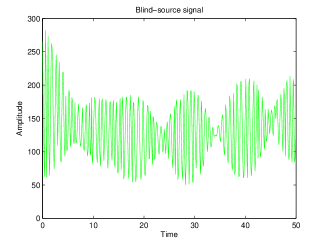
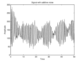
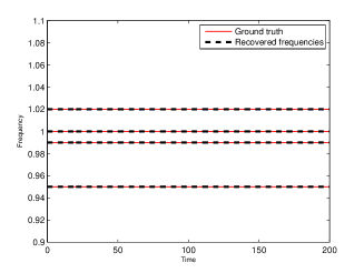
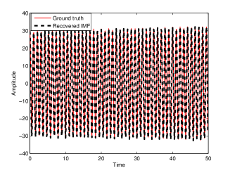
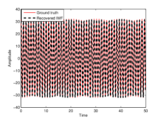
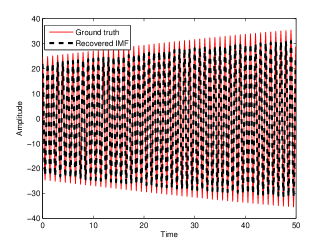
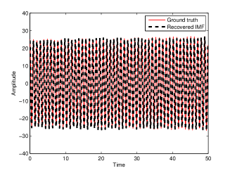
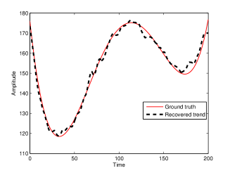
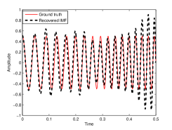
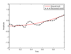
In Figure 2, we plot the original signal fI,1(t)subscript𝑓𝐼1𝑡f_{I,1}(t) and the observed signal (SNR=20absent20=20dB), together with the reconstructed results of IMFs (0<t<500𝑡500<t<50) and trend (0<t<2000𝑡2000<t<200).

Refer to caption Refer to caption Refer to caption
Refer to caption Refer to caption
Figure 2: Top (left to right): blind-source signal fI,1(t)subscript𝑓𝐼1𝑡f_{I,1}(t), fI,1(t)subscript𝑓𝐼1𝑡f_{I,1}(t) with additive noise, recovered frequencies. Middle (left to right): recovered 111st, 222nd, 333rd IMFs. Bottom (left to right): recovered 444th IMF, recovered trend.

The numerical errors in the recovery are listed in Table 1.

Table 1: Reconstructed results of Examples 13similar-to131\sim 3
Size of non-uniform samples (test data) NMSE (STD) of reconstructed IFs NMSE (STD) of reconstructed IMFs
f1,1(t)subscript𝑓11𝑡f_{1,1}(t)                 133413341334  (2000)2000(2000)         1.37×1061.37superscript1061.37\times 10^{-6}  (2.84×10⁸)2.84superscript108(2.84\times 10^{-8})         1.90×1031.90superscript1031.90\times 10^{-3}  (6.77×10⁴)6.77superscript104(6.77\times 10^{-4})
f1,2(t)subscript𝑓12𝑡f_{1,2}(t)                 133413341334  (2000)2000(2000)         1.26×1061.26superscript1061.26\times 10^{-6}  (1.10×10⁸)1.10superscript108(1.10\times 10^{-8})         2.60×1032.60superscript1032.60\times 10^{-3}  (8.70×10⁴)8.70superscript104(8.70\times 10^{-4})
f1,3(t)subscript𝑓13𝑡f_{1,3}(t)                 133413341334  (2000)2000(2000)         7.44×1067.44superscript1067.44\times 10^{-6}  (3.56×10⁸)3.56superscript108(3.56\times 10^{-8})         1.71×1021.71superscript1021.71\times 10^{-2}  (2.30×10³)2.30superscript103(2.30\times 10^{-3})
f1,4(t)subscript𝑓14𝑡f_{1,4}(t)                 133413341334  (2000)2000(2000)         2.59×1062.59superscript1062.59\times 10^{-6}  (1.97×10⁸)1.97superscript108(1.97\times 10^{-8})         1.50×1031.50superscript1031.50\times 10^{-3}  (5.44×10⁴)5.44superscript104(5.44\times 10^{-4})
A1,0(t)subscript𝐴10𝑡A_{1,0}(t)                 133413341334  (2000)2000(2000)                       similar-to\sim         2.08×1042.08superscript1042.08\times 10^{-4}  (1.51×10⁴)1.51superscript104(1.51\times 10^{-4})
f2,1(t)subscript𝑓21𝑡f_{2,1}(t)                 133513351335  (2002)2002(2002)         4.90×1044.90superscript1044.90\times 10^{-4}  (1.35×10⁴)1.35superscript104(1.35\times 10^{-4})         3.44×1023.44superscript1023.44\times 10^{-2}  (8.10×10³)8.10superscript103(8.10\times 10^{-3})
f2,2(t)subscript𝑓22𝑡f_{2,2}(t)                 133513351335  (2002)2002(2002)         6.63×1046.63superscript1046.63\times 10^{-4}  (1.71×10⁴)1.71superscript104(1.71\times 10^{-4})         6.92×1026.92superscript1026.92\times 10^{-2}  (6.70×10³)6.70superscript103(6.70\times 10^{-3})
A2,0(t)subscript𝐴20𝑡A_{2,0}(t)                 133513351335  (2002)2002(2002)                       similar-to\sim         6.30×1046.30superscript1046.30\times 10^{-4}  (2.57×10⁴)2.57superscript104(2.57\times 10^{-4})
f3,1(t)subscript𝑓31𝑡f_{3,1}(t)                 750750750   (1000)1000(1000)         7.22×1047.22superscript1047.22\times 10^{-4}  (7.46×10⁵)7.46superscript105(7.46\times 10^{-5})         3.14×1023.14superscript1023.14\times 10^{-2}  (1.80×10³)1.80superscript103(1.80\times 10^{-3})
f3,2(t)subscript𝑓32𝑡f_{3,2}(t)                 750750750   (1000)1000(1000)         1.97×1051.97superscript1051.97\times 10^{-5}  (1.43×10⁶)1.43superscript106(1.43\times 10^{-6})         2.30×1022.30superscript1022.30\times 10^{-2}  (3.10×10³)3.10superscript103(3.10\times 10^{-3})
f3,3(t)subscript𝑓33𝑡f_{3,3}(t)                 750750750   (1000)1000(1000)         2.98×1052.98superscript1052.98\times 10^{-5}  (1.80×10⁶)1.80superscript106(1.80\times 10^{-6})         2.79×1022.79superscript1022.79\times 10^{-2}  (1.38×10³)1.38superscript103(1.38\times 10^{-3})
f3,4(t)subscript𝑓34𝑡f_{3,4}(t)                 750750750   (1000)1000(1000)         7.57×1057.57superscript1057.57\times 10^{-5}  (3.56×10⁴)3.56superscript104(3.56\times 10^{-4})         4.19×1024.19superscript1024.19\times 10^{-2}  (6.20×10³)6.20superscript103(6.20\times 10^{-3})
A3,0(t)subscript𝐴30𝑡A_{3,0}(t)                 750750750   (1000)1000(1000)                       similar-to\sim         4.54×1054.54superscript1054.54\times 10^{-5}  (8.96×10⁶)8.96superscript106(8.96\times 10^{-6})

Example 5.2.

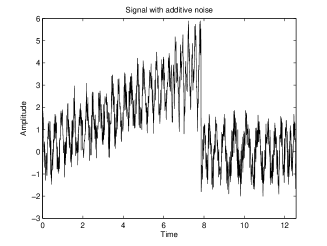
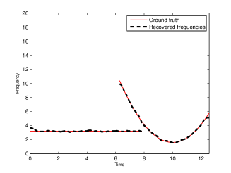
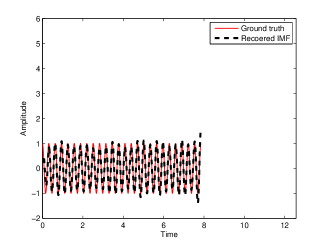
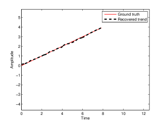
(Split signal) Next, we consider a challenging example introduced in [9], defined by

fI,2(t)=f2,1(t)+f2,2(t)+A2,0(t),subscript𝑓𝐼2𝑡subscript𝑓21𝑡subscript𝑓22𝑡subscript𝐴20𝑡\displaystyle f_{I,2}(t)=f_{2,1}(t)+f_{2,2}(t)+A_{2,0}(t), (5.7)

where

f2,1(t)=cos(2π(10t/π)),0<t<5π/2,formulae-sequencesubscript𝑓21𝑡2𝜋10𝑡𝜋0𝑡5𝜋2\displaystyle f_{2,1}(t)=\cos(2\pi(10t/\pi)),~{}~{}0<t<5\pi/2, (5.8)
f2,2(t)=cos(2π((2/3π)((t10)3(2π10)3)+(5/π)(t2π))),2π<t<4π,formulae-sequencesubscript𝑓22𝑡2𝜋23𝜋superscript𝑡103superscript2𝜋1035𝜋𝑡2𝜋2𝜋𝑡4𝜋\displaystyle f_{2,2}(t)=\cos(2\pi((2/3\pi)((t-10)^{3}-(2\pi-10)^{3})+(5/\pi)(t-2\pi))),~{}~{}2\pi<t<4\pi,
A2,0(t)=t/2,0<t<5π/2,formulae-sequencesubscript𝐴20𝑡𝑡20𝑡5𝜋2\displaystyle A_{2,0}(t)=t/2,~{}~{}0<t<5\pi/2,

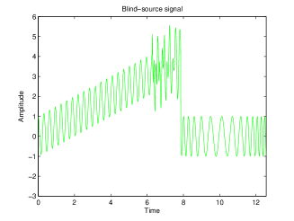
and add a noise with SNR=10absent10=10dB to this signal. This signal does not satisfy the conditions of Theorem 2.1. Nevertheless, the quasi-interpolatory spline approximation being highly localized, our techniques are able to recover the IFs and IMFs accurately as indicated in Figure 3 and reported on in further detail in Table 1.
Refer to caption Refer to caption Refer to caption
Figure 3: Top (left to right): blind-source signal fI,2(t)subscript𝑓𝐼2𝑡f_{I,2}(t), fI,2(t)subscript𝑓𝐼2𝑡f_{I,2}(t) with additive noise, recovered frequencies. Middle (left to right): recovered 111st IMF, recovered 222nd IMF, Bottom: recovered trend.

Example 5.3.

(Variable amplitudes) In this example, we illustrate the proposed method when applied to a non-stationary signal; i.e., a signal where the amplitudes are also time-dependent in addition to the frequencies, defined by

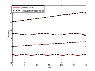
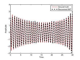
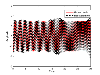
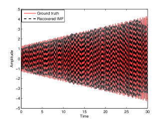
fI,3(t)=f3,1(t)+f3,2(t)+f3,3(t)+f3,4(t)+A3,0(t),0<t<30,formulae-sequencesubscript𝑓𝐼3𝑡subscript𝑓31𝑡subscript𝑓32𝑡subscript𝑓33𝑡subscript𝑓34𝑡subscript𝐴30𝑡0𝑡30\displaystyle f_{I,3}(t)=f_{3,1}(t)+f_{3,2}(t)+f_{3,3}(t)+f_{3,4}(t)+A_{3,0}(t),~{}~{}0<t<30, (5.9)

where

f3,1(t)=exp((1t/30)2+(t/30)3)cos(2π(t+cos(t)/10)),subscript𝑓31𝑡superscript1𝑡302superscript𝑡3032𝜋𝑡𝑡10\displaystyle f_{3,1}(t)=\exp((1-t/30)^{2}+(t/30)^{3})\cos(2\pi(t+\cos(t)/10)), (5.10)
f3,2(t)=(3/2)cos(2π(2t+t2/100)),subscript𝑓32𝑡322𝜋2𝑡superscript𝑡2100\displaystyle f_{3,2}(t)=(3/2)\cos(2\pi(2t+t^{2}/100)),
f3,3(t)=(t/10+13/10)cos(2π(7t/2+sin(t/2)/5)),subscript𝑓33𝑡𝑡1013102𝜋7𝑡2𝑡25\displaystyle f_{3,3}(t)=(t/10+13/10)\cos(2\pi(7t/2+\sin(t/2)/5)),
f3,4(t)=(1+cos(πt/50)/2)cos(2π(5t+t2/50)),subscript𝑓34𝑡1𝜋𝑡5022𝜋5𝑡superscript𝑡250\displaystyle f_{3,4}(t)=(1+\cos(\pi t/50)/2)\cos(2\pi(5t+t^{2}/50)),
A3,0(t)=(64/5)((t15)/16)4(64/5)((t15)/12)2+4t/5+16/5.subscript𝐴30𝑡645superscript𝑡15164645superscript𝑡151224𝑡5165\displaystyle A_{3,0}(t)=(64/5)((t-15)/16)^{4}-(64/5)((t-15)/12)^{2}+4t/5+16/5.

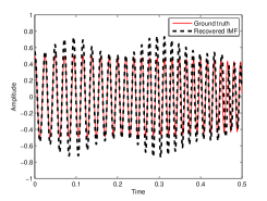
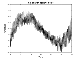
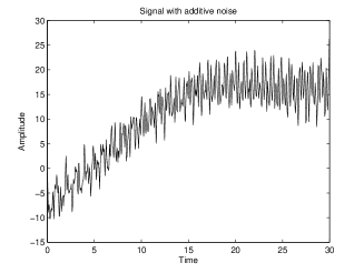
The signal fI,3(t)subscript𝑓𝐼3𝑡f_{I,3}(t) is added with a white noise with SNR=25absent25=25dB. The results are illustrated graphically in Figure 4, with details given in Table 1.
Refer to caption Refer to caption Refer to caption
Refer to caption Refer to caption
Figure 4: Top (left to right): blind-source signal fI,3(t)subscript𝑓𝐼3𝑡f_{I,3}(t), fI,3(t)subscript𝑓𝐼3𝑡f_{I,3}(t) with additive noise, recovered frequencies. Middle (left to right): recovered 111st IMF, recovered 222nd IMF, recovered 333rd IMF. Bottom: recovered 444th IMF, recovered trend.

Example 5.4.

(Robustness) The following example demonstrates the robustness of our method.

fI,4(t)=f4,1(t)+f4,2(t)+A4,0(t),0<t<1,formulae-sequencesubscript𝑓𝐼4𝑡subscript𝑓41𝑡subscript𝑓42𝑡subscript𝐴40𝑡0𝑡1\displaystyle f_{I,4}(t)=f_{4,1}(t)+f_{4,2}(t)+A_{4,0}(t),~{}~{}0<t<1, (5.11)

where

f4,1(t)=(1/2)exp((t1/2)2/50)cos(2π(20t+25t2)),subscript𝑓41𝑡12superscript𝑡122502𝜋20𝑡25superscript𝑡2\displaystyle f_{4,1}(t)=(1/2)\exp(-(t-1/2)^{2}/50)\cos(2\pi(20t+25t^{2})), (5.12)
f4,2(t)=(1/4)(1+cos(πt/2))cos(2π(40t+25t2)),subscript𝑓42𝑡141𝜋𝑡22𝜋40𝑡25superscript𝑡2\displaystyle f_{4,2}(t)=(1/4)(1+\cos(\pi t/2))\cos(2\pi(40t+25t^{2})),
A4,0(t)=t2.subscript𝐴40𝑡superscript𝑡2\displaystyle A_{4,0}(t)=t^{2}.

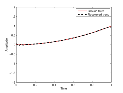
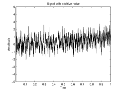
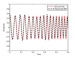
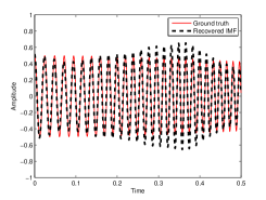
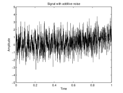
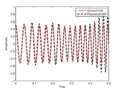
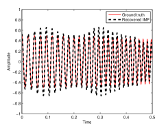
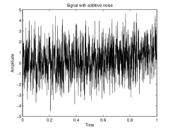
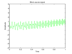
To sufficiently analyze the robustness, we use our method with the pure blind source signal fI,4(t)subscript𝑓𝐼4𝑡f_{I,4}(t) and again the signal added with various levels of white noise (SNR=0,5,8absent058=0,-5,-8). The reconstructed results of signals with different noise levels are shown graphically in Figure 5 and and numerically in Table 2.
Refer to caption Refer to caption Refer to caption Refer to caption
Figure 5: Top (left to right): blind-source signal fI,4(t)subscript𝑓𝐼4𝑡f_{I,4}(t), recovered 1st IMF, recovered 2nd IMF, recovered trend. Second row (left to right): fI,4(t)subscript𝑓𝐼4𝑡f_{I,4}(t) with additive noise (SNR=0), recovered 1st IMF, recovered 2nd IMF, recovered trend. Third row (left to right): fI,4(t)subscript𝑓𝐼4𝑡f_{I,4}(t) with additive noise (SNR=-5), recovered 1st IMF, recovered 2nd IMF, recovered trend. Bottom: (left to right): fI,4(t)subscript𝑓𝐼4𝑡f_{I,4}(t) with additive noise (SNR=-8), recovered 1st IMF, recovered 2nd IMF , recovered trend.
Table 2: Reconstructed results of Examples 444
Size of non-uniform samples (test data) NMSE (STD) of reconstructed IFs NMSE (STD) of reconstructed IMFs
f4,1(t)subscript𝑓41𝑡f_{4,1}(t)                 150015001500  (2000)2000(2000)         5.31×1055.31superscript1055.31\times 10^{-5}  (3.84×10¹⁰)3.84superscript1010(3.84\times 10^{-10})         3.18×1023.18superscript1023.18\times 10^{-2}  (1.42×10⁵)1.42superscript105(1.42\times 10^{-5})
f4,2(t)subscript𝑓42𝑡f_{4,2}(t)                 150015001500  (2000)2000(2000)         2.82×1052.82superscript1052.82\times 10^{-5}  (7.88×10⁸)7.88superscript108(7.88\times 10^{-8})         3.19×1023.19superscript1023.19\times 10^{-2}  (7.11×10⁵)7.11superscript105(7.11\times 10^{-5})
A4,0(t)subscript𝐴40𝑡A_{4,0}(t)                 150015001500  (2000)2000(2000)                       similar-to\sim         4.15×1044.15superscript1044.15\times 10^{-4}  (5.26×10⁶)5.26superscript106(5.26\times 10^{-6})
f4,1(t)subscript𝑓41𝑡f_{4,1}(t)                 150015001500  (2000)2000(2000)         1.60×1041.60superscript1041.60\times 10^{-4}  (1.70×10⁵)1.70superscript105(1.70\times 10^{-5})         6.24×1026.24superscript1026.24\times 10^{-2}  (1.12×10²)1.12superscript102(1.12\times 10^{-2})
f4,2(t)subscript𝑓42𝑡f_{4,2}(t)                 150015001500  (2000)2000(2000)         1.81×1041.81superscript1041.81\times 10^{-4}  (1.60×10⁵)1.60superscript105(1.60\times 10^{-5})         7.84×1027.84superscript1027.84\times 10^{-2}  (1.37×10²)1.37superscript102(1.37\times 10^{-2})
A4,0(t)subscript𝐴40𝑡A_{4,0}(t)                 150015001500  (2000)2000(2000)                       similar-to\sim         1.06×1021.06superscript1021.06\times 10^{-2}  (1.55×10³)1.55superscript103(1.55\times 10^{-3})
f4,1(t)subscript𝑓41𝑡f_{4,1}(t)                 150015001500  (2000)2000(2000)         1.61×1021.61superscript1021.61\times 10^{-2}  (5.00×10³)5.00superscript103(5.00\times 10^{-3})         1.62×1011.62superscript1011.62\times 10^{-1}  (2.63×10²)2.63superscript102(2.63\times 10^{-2})
f4,2(t)subscript𝑓42𝑡f_{4,2}(t)                 150015001500  (2000)2000(2000)         1.14×1021.14superscript1021.14\times 10^{-2}  (4.90×10³)4.90superscript103(4.90\times 10^{-3})         3.11×1013.11superscript1013.11\times 10^{-1}  (8.29×10²)8.29superscript102(8.29\times 10^{-2})
A4,0(t)subscript𝐴40𝑡A_{4,0}(t)                 150015001500  (2000)2000(2000)                       similar-to\sim         2.37×1022.37superscript1022.37\times 10^{-2}  (6.10×10³)6.10superscript103(6.10\times 10^{-3})
f4,1(t)subscript𝑓41𝑡f_{4,1}(t)                 150015001500  (2000)2000(2000)         3.15×1023.15superscript1023.15\times 10^{-2}  (9.00×10³)9.00superscript103(9.00\times 10^{-3})         4.09×1014.09superscript1014.09\times 10^{-1}  (5.47×10²)5.47superscript102(5.47\times 10^{-2})
f4,2(t)subscript𝑓42𝑡f_{4,2}(t)                 150015001500  (2000)2000(2000)         1.72×1021.72superscript1021.72\times 10^{-2}  (5.70×10³)5.70superscript103(5.70\times 10^{-3})         6.54×1016.54superscript1016.54\times 10^{-1}  (1.49×101)1.49superscript101(1.49\times 10^{-1})
A4,0(t)subscript𝐴40𝑡A_{4,0}(t)                 150015001500  (2000)2000(2000)                       similar-to\sim         4.73×1024.73superscript1024.73\times 10^{-2}  (1.25×10²)1.25superscript102(1.25\times 10^{-2})

Example 5.5.

(Extrapolation) Our aim in this example is to examine the utility of our methods in extrapolating the signal a little bit beyond the time interval where its values are available, both in the past and in the future. We consider

fI,5(t)=f5,1(t)+f5,2(t)+A5,0(t),0<t<30,formulae-sequencesubscript𝑓𝐼5𝑡subscript𝑓51𝑡subscript𝑓52𝑡subscript𝐴50𝑡0𝑡30\displaystyle f_{I,5}(t)=f_{5,1}(t)+f_{5,2}(t)+A_{5,0}(t),~{}~{}0<t<30, (5.13)

where

f5,1(t)=exp(2(t/30)2t/15+1)cos(2π(2t+0.01t2)),subscript𝑓51𝑡2superscript𝑡302𝑡1512𝜋2𝑡0.01superscript𝑡2\displaystyle f_{5,1}(t)=\exp(2(t/30)^{2}-t/15+1)\cos(2\pi(2t+0.01t^{2})), (5.14)
f5,2(t)=(1+4(t/30)2+3(1t/30)3)cos(2π(4t+0.01t2)),subscript𝑓52𝑡14superscript𝑡3023superscript1𝑡3032𝜋4𝑡0.01superscript𝑡2\displaystyle f_{5,2}(t)=(1+4(t/30)^{2}+3(1-t/30)^{3})\cos(2\pi(4t+0.01t^{2})),
A5,0(t)=t3/10047t2/100+27t/59.subscript𝐴50𝑡superscript𝑡310047superscript𝑡210027𝑡59\displaystyle A_{5,0}(t)=t^{3}/100-47t^{2}/100+27t/5-9.

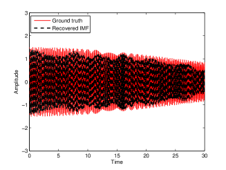
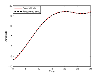
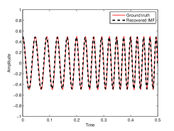
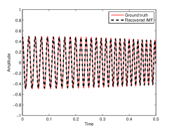
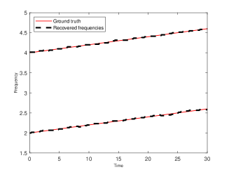
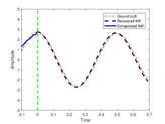
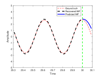
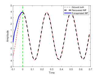
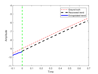
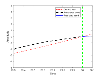
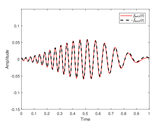
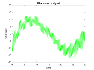
To verify that our approach applies to data extrapolation, we process the data on the time-interval [0,30]030[0,30], and predict the value of the IFs, IMFs, and the trend on the interval [0.1,30.1]0.130.1[-0.1,30.1]; i.e., for 0.10.10.1 time units in the past and the same in the future. To demonstrate that our extrapolated graphs are good approximation of the unknown ground truth, we zoom-in to the intervals [0.1,0.7]0.10.7[-0.1,0.7] and [29.3,30.1]29.330.1[29.3,30.1]. The results are shown graphically in Figure 6.
Refer to caption Refer to caption Refer to caption
Figure 6: Top (left to right): blind-source signal fI,5(t)subscript𝑓𝐼5𝑡f_{I,5}(t), fI,5(t)subscript𝑓𝐼5𝑡f_{I,5}(t) with additive noise, recovered frequencies. In the second and third rows, we zoom-in to the sub-intervals [0,0.7]00.7[0,0.7] and [29.3,30]29.330[29.3,30] and extrapolate the data outside the time domain to [0.1,0]0.10[-0.1,0] and [30,30.1]3030.1[30,30.1], respectively. Middle (left to right): Extrapolated 111st IMF, predicted 111st IMF, extrapolated 222nd IMF. Bottom (left to right): Predicted 222nd IMF, extrapolated trend, predicted trend.

Example 5.6.

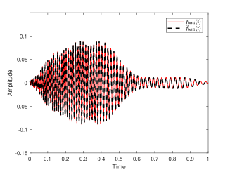
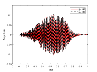
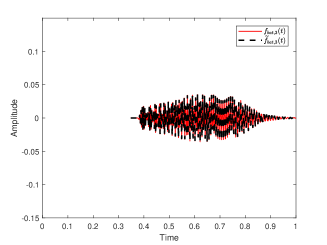
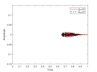
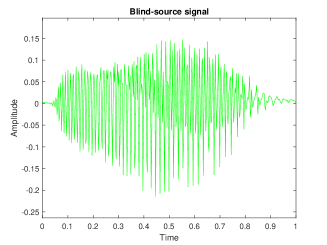
(Bat Echo-location) We consider a real-word signal, namely “a bat echolocation signal” fbatsubscript𝑓batf_{{\rm bat}} 111http://dsp.rice.edu/software/bat-echolocation-chirp emitted by a large brown bat, and discover that it consists of four IMFs,

fI,bat=fbat,1+fbat,2+fbat,3+fbat,4.subscript𝑓𝐼batsubscript𝑓bat1subscript𝑓bat2subscript𝑓bat3subscript𝑓bat4\displaystyle f_{I,{\rm bat}}=f_{{\rm bat},1}+f_{{\rm bat},2}+f_{{\rm bat},3}+f_{{\rm bat},4}.

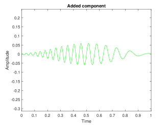
To convince ourselves that this decomposition makes sense, we add an unknown signal fbat,5subscript𝑓bat5f_{{\rm bat},5}, given by

fbat,5(t)=(4/125(7/254)cos(2πt))cos(2π(30t13t2)),subscript𝑓bat5𝑡412572542𝜋𝑡2𝜋30𝑡13superscript𝑡2\displaystyle f_{{\rm bat},5}(t)=(4/125-(7/254)\cos(2\pi t))\cos(2\pi(30t-13t^{2})),

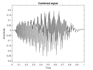
to fI,batsubscript𝑓𝐼batf_{I,{\rm bat}} and decompose the combined blind source signal fI,bat+fbat,5subscript𝑓𝐼batsubscript𝑓bat5f_{I,{\rm bat}}+f_{{\rm bat},5}, and discover that it consists of five IMFs, f~bat,1subscript~𝑓bat1\widetilde{f}_{{\rm bat},1}, f~bat,2subscript~𝑓bat2\widetilde{f}_{{\rm bat},2},…, f~bat,5subscript~𝑓bat5\widetilde{f}_{{\rm bat},5}. The MSEs of the five IMFs are 2.26×1042.26superscript1042.26\times 10^{-4}, 1.10×1041.10superscript1041.10\times 10^{-4}, 1.49×1041.49superscript1041.49\times 10^{-4}, 7.67×1047.67superscript1047.67\times 10^{-4}, and 1.74×1021.74superscript1021.74\times 10^{-2}, respectively, where MSE is measured by fbat,if~bat,i22/fbat,i22.superscriptsubscriptnormsubscript𝑓bat𝑖subscript~𝑓bat𝑖22superscriptsubscriptnormsubscript𝑓bat𝑖22\|f_{{\rm bat},i}-\widetilde{f}_{{\rm bat},i}\|_{2}^{2}/\|f_{{\rm bat},i}\|_{2}^{2}. Through the comparison of recovery, it demonstrates that the proposed computational scheme can recover the IMFs effectively. Furthermore, it enables us to identity and quantify the blind-source signal through efficient extraction of information from the individual components.
Refer to caption Refer to caption Refer to caption
Refer to caption Refer to caption
Figure 7: Top (left to right): blind-source signal, added component fbat,5(t)subscript𝑓𝑏𝑎𝑡5𝑡f_{bat,5}(t), combined signal. Middle (left to right): recovered 111st IMF, recovered 222nd IMF, recovered 333rd IMF. Bottom (left to right): recovered 444th IMF, recovered 555th IMF.

6 Conclusions

In this paper, we have developed a rigorous theory, along with an effective algorithm and efficient computational scheme, for the construction of deep networks to resolving the problem of separation of signal components and extraction of their instantaneous frequencies, based on random, non-uniform samples of a blind-source composite signal on a bounded time interval. This provides an effective solution of an important problem in signal processing, that none of the existing methods, including the popular empirical mode decomposition (EMD), synchrosqueezed wavelet transform (SST), as well as our previous signal separation operation (SSO), could work satisfactorily in general. A highlight of our computational procedure is that it precisely determines the exact number of signal components without an a priori knowledge of the composite signal. In addition, our deep networks are “theory inspired”; i.e., constructed on the basis of a solid mathematical theory which allows the use of pre-fabricated networks that do not require training in the classical sense. Our results are proved mathematically as well as demonstrated experimentally, including an example of real-world bat echo-location signal.

References

  • [1] G. Chen, C. K. Chui, and M. Lai. Construction of real-time spline quasiinterpolation schemes. Approx. Theory Appl, 4(4):61–75, 1988.
  • [2] C. K. Chui. Multivariate splines. SIAM, 1988.
  • [3] C. K. Chui. An introduction to wavelets. Academic press, San Diego, 1992.
  • [4] C. K. Chui and H. Diamond. A general framework for local interpolation. Numerische Mathematik, 58(1):569–581, 1990.
  • [5] C. K. Chui, Y.-T. Lin, and H.-T. Wu. Real-time dynamics acquisition from irregular samples—with application to anesthesia evaluation. Analysis and Applications, 14(04):537–590, 2016.
  • [6] C. K. Chui and H. N. Mhaskar. Signal decomposition and analysis via extraction of frequencies. Applied and Computational Harmonic Analysis, 40(1):97–136, 2016.
  • [7] C. K. Chui, H. N. Mhaskar, and M. D. van der Walt. Data-driven atomic decomposition via frequency extraction of intrinsic mode functions. GEM-International Journal on Geomathematics, 7(1):117–146, 2016.
  • [8] C. K. Chui and M. D. van der Walt. Signal analysis via instantaneous frequency estimation of signal components. GEM-International Journal on Geomathematics, 6(1):1–42, 2015.
  • [9] I. Daubechies, J. Lu, and H. T. Wu. Synchrosqueezed wavelet transforms: an empirical mode decomposition-like tool. Applied and computational harmonic analysis, 30(2):243–261, 2011.
  • [10] I. Daubechies and S. Maes. A nonlinear squeezing of the continuous wavelet transform based on auditory nerve models. Wavelets in medicine and biology, pages 527–546, 1996.
  • [11] C. de Boor. A practical guide to splines. Springer Verlag., 1978.
  • [12] C. de Boor and G. Fix. Spline approximation by quasiinterpolants. Journal of Approximation Theory, 8(1):19–45, 1973.
  • [13] B. G. R. De Prony. Essai éxperimental et analytique: sur les lois de la dilatabilité de fluides élastique et sur celles de la force expansive de la vapeur de l’alkool,a différentes températures. Journal de l’école polytechnique, 1(22):24–76, 1795.
  • [14] N. E. Huang, Z. Shen, S. R. Long, M. C. Wu, H. H. Shih, Q. Zheng, N. Yen, C. C. Tung, and H. H. Liu. The empirical mode decomposition and the Hilbert spectrum for nonlinear and non-stationary time series analysis. Proceedings of the Royal Society of London. Series A: Mathematical, Physical and Engineering Sciences, 454(1971):903–995, 1998.
  • [15] H. N. Mhaskar. Approximation properties of a multilayered feedforward artificial neural network. Advances in Computational Mathematics, 1(1):61–80, 1993.
  • [16] H. N. Mhaskar and C. A. Micchelli. Degree of approximation by neural and translation networks with a single hidden layer. Advances in Applied Mathematics, 16(2):151–183, 1995.
  • [17] G. Thakur and H. T. Wu. Synchrosqueezing-based recovery of instantaneous frequency from nonuniform samples. SIAM Journal on Mathematical Analysis, 43(5):2078–2095, 2011.
  • [18] M. D. van der Walt. Wavelet Analysis of Non-stationary Signals with Applications. PhD thesis, University of Missouri, St. Louis, 2015.
  • [19] H.-T. Wu. Adaptive Analysis of Complex Data Sets. PhD thesis, Princeton University, 2012.
  • [20] H. T. Wu, P. Flandrin, and I. Daubechies. One or two frequencies? the synchrosqueezing answers. Advances in Adaptive Data Analysis, 3(01n02):29–39, 2011.