Consensus-Based Optimization on Hypersurfaces: Well-Posedness and Mean-Field Limit

Massimo Fornasier 111Department of Mathematics, Technical University of Munich, Boltzmannstraße 3, 85748 Garching (Munich), Germany (massimo.fornasier@ma.tum.de).  Hui Huang 222Department of Mathematics, Technical University of Munich, Boltzmannstraße 3, 85748 Garching (Munich), Germany (hui.huang@tum.de).  Lorenzo Pareschi333Department of Mathematics & Computer Science, University of Ferrara, Via Machiavelli 30, Ferrara, 44121, Italy (lorenzo.pareschi@unife.it).  Philippe Sünnen 444Department of Mathematics, Technical University of Munich, Boltzmannstraße 3, 85748 Garching (Munich), Germany (philippe.suennen@ma.tum.de).
Abstract

We introduce a new stochastic differential model for global optimization of nonconvex functions on compact hypersurfaces. The model is inspired by the stochastic Kuramoto-Vicsek system and belongs to the class of Consensus-Based Optimization methods. In fact, particles move on the hypersurface driven by a drift towards an instantaneous consensus point, computed as a convex combination of the particle locations weighted by the cost function according to Laplace’s principle. The consensus point represents an approximation to a global minimizer. The dynamics is further perturbed by a random vector field to favor exploration, whose variance is a function of the distance of the particles to the consensus point. In particular, as soon as the consensus is reached, then the stochastic component vanishes. In this paper, we study the well-posedness of the model and we derive rigorously its mean-field approximation for large particle limit.

Keywords: Consensus-based optimization, optimization over manifolds, stochastic Kuramoto-Vicsek model, well-posedness, mean-field limit

1 Introduction

Over the last decades, large systems of interacting particles (or agents) are widely used to investigate self-organization and collective behavior. They frequently appear in modeling phenomena such as biological swarms [14, 18], crowd dynamics [2, 7, 8], self-assembly of nanoparticles [38] and opinion formation [3, 47, 35]. Similar particle models are also used in metaheuristics [1, 6, 10, 31], which provide empirically robust solutions to tackle hard optimization problems with fast algorithms. Metaheuristics are methods that orchestrate an interaction between local improvement procedures and global/high level strategies, and combine random and deterministic decisions, to create a process capable of escaping from local optima and performing a robust search of a solution space. Starting with the groundbreaking work Ref. [51] of Rastrigin on Random Search in 1963, numerous mechanisms for multi-agent global optimization have been considered, among the most prominent instances we recall the Simplex Heuristics [48], Evolutionary Programming [28], the Metropolis-Hastings sampling algorithm [34], Genetic Algorithms [36], Particle Swarm Optimization (PSO) [41, 50], Ant Colony Optimization (ACO) [23] and Simulated Annealing (SA) [37, 42]. Despite the tremendous empirical success of these techniques, most metaheuristical methods still lack proper mathematical proof of robust convergence to global minimizers. In fact, due to the random component of metaheuristics, their asymptotic analysis would require to discern the stochastic dependencies, which is a daunting task, especially for those methods that combine instantaneous decisions with memory mechanisms.

Recent work Refs. [49, 13] on Consensus-Based Optimization (CBO) focuses on instantaneous stochastic and deterministic decisions in order to establish a consensus among particles on the location of the global minimizers within a domain. In view of the instantaneous nature of the dynamics, the evolution of the system can be interpreted as a system of first order stochastic differential equations, whose large particle limit is approximated by a deterministic partial differential equation of mean-field type. The large time behavior of such a deterministic PDE can be analyzed by classical techniques of large deviation bounds and the global convergence of the mean-field model can be mathematically proven in a rigorous way for a large class of optimization problems. Certainly CBO is a significantly simpler mechanism with respect to more sophisticated metaheuristics, which can include different features including memory of past exploration. Nevertheless, it seems to be powerful and robust enough to tackle many interesting nonconvex optimizations [15, 29, 33], which would be harder to solve by gradient descent methods that have been dominating the field of optimization, especially in relevant applications such as machine learning. In fact in many of these problems the objective function is not differentiable and CBO do not use any gradient information for their exploration. Moreover, in certain models, such as training of deep neural networks, the gradient tends to explode or vanish [9]. Finally, although there exist situations where global optimization by gradient descent methods can be ensured under ad hoc conditions, see, e.g. Refs. [16, 45, 44], they do not offer in general guarantees of global convergence. Instead, CBO has potential of a rather general and rigorous global asymptotic/convergence analysis. Some theoretical gaps remain open in the analysis of CBO though, in particular the rigorous derivation of the mean-field limit, due to the difficulty in establishing bounds on the moments of the probability distribution of the particles [13]. Because of this lack of compactness, a direct proof of convergence of the stochastic particle method has been recently derived in Ref. [33], which does not require the mean-field limit, but at the same time it is not able to provide a quantitative error estimate with respect to the number of particles.

Motivated by these theoretical gaps and several potential applications in machine learning, the main task of the present work is to develop a CBO approach to solve the following constrained optimization problem

vargminvΓ(v),superscript𝑣argsubscript𝑣Γ𝑣v^{\ast}\in{\rm arg}\!\min\limits_{v\in\Gamma}\mathcal{E}(v)\,, (1.1)

where 0:d:0superscript𝑑0\leq\mathcal{E}:\mathbb{R}^{d}\to\mathbb{R} is a given continuous cost function, which we wish to minimize over a hypersurface ΓΓ\Gamma. Here we assume that ΓΓ\Gamma is a connected smooth compact hypersurface embedded in dsuperscript𝑑\mathbb{R}^{d}, which is represented as the 00-level set of a signed distance function γ𝛾\gamma with |γ(v)|=dist(v,Γ)𝛾𝑣dist𝑣Γ|\gamma(v)|=\mbox{dist}(v,\Gamma). This means that

Γ={vd|γ(v)=0}.Γconditional-set𝑣superscript𝑑𝛾𝑣0\Gamma=\left\{v\in\mathbb{R}^{d}|\leavevmode\nobreak\ \gamma(v)=0\right\}\,.

If Γ=Γ\partial\Gamma=\emptyset, we also assume for simplicity that γ<0𝛾0\gamma<0 on the interior of ΓΓ\Gamma and γ>0𝛾0\gamma>0 on the exterior. The gradient γ𝛾\nabla\gamma is then the outward unit normal on ΓΓ\Gamma wherever γ𝛾\gamma is defined. Moreover, we assume that there exists an open neighborhood Γ^^Γ\widehat{\Gamma} of ΓΓ\Gamma such that γ𝒞3(Γ^)𝛾superscript𝒞3^Γ\gamma\in\mathcal{C}^{3}(\widehat{\Gamma}). Such setting of hypersurface ΓΓ\Gamma has been used in Ref. [22].

Example 1.1.

Examples of hypersurfaces ΓΓ\Gamma in this setting are

  • the unit sphere SSd1superscriptSS𝑑1\SS^{d-1}, in which case γ(v)=|v|1𝛾𝑣𝑣1\gamma(v)=|v|-1, γ(v)=v|v|𝛾𝑣𝑣𝑣\nabla\gamma(v)=\frac{v}{|v|} and Δγ(v)=d1|v|Δ𝛾𝑣𝑑1𝑣\Delta\gamma(v)=\frac{d-1}{|v|};

  • a torus radially symmetric about the vdsuperscript𝑣𝑑v^{d}-axis and of inner radius r>0𝑟0r>0 and external radius R>0𝑅0R>0 that is expressed in Cartesian coordinates as the 00-level set of the signed distance function γ(v)=(|v|2(vd)2R)2+(vd)2r𝛾𝑣superscriptsuperscript𝑣2superscriptsuperscript𝑣𝑑2𝑅2superscriptsuperscript𝑣𝑑2𝑟\gamma(v)=\sqrt{(\sqrt{|v|^{2}-(v^{d})^{2}}-R)^{2}+(v^{d})^{2}}-r, where v=(v1,,vd)𝑣superscript𝑣1superscript𝑣𝑑v=(v^{1},\dots,v^{d}).

In particular, we consider a system of N𝑁N interacting particles ((Vti)t0)i=1,,Nsubscriptsubscriptsuperscriptsubscript𝑉𝑡𝑖𝑡0𝑖1𝑁((V_{t}^{i})_{t\geq 0})_{i=1,\dots,N} satisfying the following stochastic differential dynamics expressed in Itô’s form

dVti𝑑superscriptsubscript𝑉𝑡𝑖\displaystyle dV_{t}^{i} =λP(Vti)(Vtivα,(ρtN))dt+σ|Vtivα,(ρtN)|P(Vti)dBtiσ22(Vtivα,(ρtN))2Δγ(Vti)γ(Vti)dt,absent𝜆𝑃superscriptsubscript𝑉𝑡𝑖superscriptsubscript𝑉𝑡𝑖subscript𝑣𝛼superscriptsubscript𝜌𝑡𝑁𝑑𝑡𝜎superscriptsubscript𝑉𝑡𝑖subscript𝑣𝛼superscriptsubscript𝜌𝑡𝑁𝑃superscriptsubscript𝑉𝑡𝑖𝑑superscriptsubscript𝐵𝑡𝑖superscript𝜎22superscriptsuperscriptsubscript𝑉𝑡𝑖subscript𝑣𝛼superscriptsubscript𝜌𝑡𝑁2Δ𝛾superscriptsubscript𝑉𝑡𝑖𝛾superscriptsubscript𝑉𝑡𝑖𝑑𝑡\displaystyle=-\lambda P(V_{t}^{i})(V_{t}^{i}-v_{\alpha,\mathcal{E}}(\rho_{t}^{N}))dt+\sigma|V_{t}^{i}-v_{\alpha,\mathcal{E}}(\rho_{t}^{N})|P(V_{t}^{i})dB_{t}^{i}-\frac{\sigma^{2}}{2}(V_{t}^{i}-v_{\alpha,\mathcal{E}}(\rho_{t}^{N}))^{2}\Delta\gamma(V_{t}^{i})\nabla\gamma(V_{t}^{i})dt\,, (1.2)

where λ>0𝜆0\lambda>0 is a suitable drift parameter, σ>0𝜎0\sigma>0 a diffusion parameter,

ρtN=1Ni=1NδVti,superscriptsubscript𝜌𝑡𝑁1𝑁superscriptsubscript𝑖1𝑁subscript𝛿superscriptsubscript𝑉𝑡𝑖\rho_{t}^{N}=\frac{1}{N}\sum_{i=1}^{N}\delta_{V_{t}^{i}}\,, (1.3)

is the empirical measure of the particles (δvsubscript𝛿𝑣\delta_{v} is the Dirac measure at vd𝑣superscript𝑑v\in\mathbb{R}^{d}), and

vα,(ρtN)=j=1NVtjeα(Vtj)j=1Neα(Vtj)=dvωα(v)𝑑ρtNdωα(v)𝑑ρtN with ωα(v):=eα(v).formulae-sequencesubscript𝑣𝛼superscriptsubscript𝜌𝑡𝑁superscriptsubscript𝑗1𝑁subscriptsuperscript𝑉𝑗𝑡superscript𝑒𝛼subscriptsuperscript𝑉𝑗𝑡superscriptsubscript𝑗1𝑁superscript𝑒𝛼subscriptsuperscript𝑉𝑗𝑡subscriptsuperscript𝑑𝑣superscriptsubscript𝜔𝛼𝑣differential-dsuperscriptsubscript𝜌𝑡𝑁subscriptsuperscript𝑑superscriptsubscript𝜔𝛼𝑣differential-dsuperscriptsubscript𝜌𝑡𝑁assign with superscriptsubscript𝜔𝛼𝑣superscript𝑒𝛼𝑣v_{\alpha,\mathcal{E}}(\rho_{t}^{N})=\frac{\sum_{j=1}^{N}V^{j}_{t}e^{-\alpha\mathcal{E}(V^{j}_{t})}}{\sum_{j=1}^{N}e^{-\alpha\mathcal{E}(V^{j}_{t})}}=\frac{\int_{\mathbb{R}^{d}}v\omega_{\alpha}^{\mathcal{E}}(v)d\rho_{t}^{N}}{\int_{\mathbb{R}^{d}}\omega_{\alpha}^{\mathcal{E}}(v)d\rho_{t}^{N}}\quad\mbox{ with }\quad\omega_{\alpha}^{\mathcal{E}}(v):=e^{-\alpha\mathcal{E}(v)}\,. (1.4)

For simplicity, we write v2superscript𝑣2v^{2} to mean |v|2superscript𝑣2|v|^{2} for any vector vd𝑣superscript𝑑v\in\mathbb{R}^{d}, and |v|𝑣|v| is the standard Euclidean norm. This stochastic system is considered complemented with independent and identical distributed (i.i.d.) initial data V0iΓsuperscriptsubscript𝑉0𝑖ΓV_{0}^{i}\in\Gamma with i=1,,N𝑖1𝑁i=1,\cdots,N, and the common law is denoted by ρ0𝒫(Γ)subscript𝜌0𝒫Γ\rho_{0}\in\mathcal{P}(\Gamma). The trajectories ((Bti)t0)i=1,Nsubscriptsubscriptsuperscriptsubscript𝐵𝑡𝑖𝑡0𝑖1𝑁((B_{t}^{i})_{t\geq 0})_{i=1,\dots N} denote N𝑁N independent standard Brownian motions in dsuperscript𝑑\mathbb{R}^{d}. In (1.2) the projection operator P()𝑃P(\cdot) is defined by

P(v)=Iγ(v)γ(v)T.𝑃𝑣𝐼𝛾𝑣𝛾superscript𝑣𝑇P(v)=I-\nabla\gamma(v)\nabla\gamma(v)^{T}\,. (1.5)

In the case of sphere we know γ(v)=v|v|𝛾𝑣𝑣𝑣\nabla\gamma(v)=\frac{v}{|v|}, so one has P(v)=IvvT|v|2𝑃𝑣𝐼𝑣superscript𝑣𝑇superscript𝑣2P(v)=I-\frac{vv^{T}}{|v|^{2}}, and (1.2) corresponds to a stochastic Kuramoto-Vicsek type model [43, 53, 12].

The choice of the weight function ωαsuperscriptsubscript𝜔𝛼\omega_{\alpha}^{\mathcal{E}} in (1.4) comes from the well-known Laplace’s principle [46, 21, 49], a classical asymptotic method for integrals, which states that for any probability measure ρ𝒫(Γ)𝜌𝒫Γ\rho\in\mathcal{P}(\Gamma), it holds555 For the sake of the reader we provide a simple argument for the validity of this well-known formula: let us take the exponential on the right-hand-side limit to obtain limα1(Γeα(v)𝑑ρ(v))1/α=(esssupvsupp(ρ)e(v))1=essinfvsupp(ρ)e(v)subscript𝛼1superscriptsubscriptΓsuperscript𝑒𝛼𝑣differential-d𝜌𝑣1𝛼superscriptesssubscriptsupremum𝑣supp𝜌superscript𝑒𝑣1esssubscriptinfimum𝑣supp𝜌superscript𝑒𝑣\lim\limits_{\alpha\to\infty}\frac{1}{\left(\int_{\Gamma}e^{-\alpha\mathcal{E}(v)}d\rho(v)\right)^{1/\alpha}}=({\rm ess}\sup_{v\in{\rm supp}(\rho)}e^{-\mathcal{E}(v)})^{-1}={\rm ess}\inf_{v\in{\rm supp}(\rho)}e^{\mathcal{E}(v)}. The first equality holds by the well-known limit of Lαsuperscript𝐿𝛼L^{\alpha}-norms to the Lsuperscript𝐿L^{\infty}-norm for which limαe()α=e()subscript𝛼subscriptnormsuperscript𝑒𝛼subscriptnormsuperscript𝑒\lim_{\alpha\to\infty}\|e^{-\mathcal{E}(\cdot)}\|_{\alpha}=\|e^{-\mathcal{E}(\cdot)}\|_{\infty}. By applying now the logarithm and using its continuity, one obtains (1.6).

limα(1αlog(Γeα(v)𝑑ρ(v)))=infvsupp(ρ)(v).subscript𝛼1𝛼subscriptΓsuperscript𝑒𝛼𝑣differential-d𝜌𝑣subscriptinfimum𝑣supp𝜌𝑣\lim\limits_{\alpha\to\infty}\left(-\frac{1}{\alpha}\log\left(\int_{\Gamma}e^{-\alpha\mathcal{E}(v)}d\rho(v)\right)\right)=\inf\limits_{v\in\rm{supp}(\rho)}\mathcal{E}(v)\,. (1.6)

Let us discuss the mechanism of the dynamics. The right-hand-side of the equation (1.2) is made of three terms. The first deterministic term λP(Vti)(Vtivα,(ρtN))dt𝜆𝑃superscriptsubscript𝑉𝑡𝑖superscriptsubscript𝑉𝑡𝑖subscript𝑣𝛼superscriptsubscript𝜌𝑡𝑁𝑑𝑡-\lambda P(V_{t}^{i})(V_{t}^{i}-v_{\alpha,\mathcal{E}}(\rho_{t}^{N}))dt imposes a drift to the dynamics towards vα,subscript𝑣𝛼v_{\alpha,\mathcal{E}}, which is the current consensus point at time t𝑡t as approximation to the global minimizer. This drift term is the projection onto the tangent space to the hypersurfaces at Vtisuperscriptsubscript𝑉𝑡𝑖V_{t}^{i} of the vector vα,Vtisubscript𝑣𝛼superscriptsubscript𝑉𝑡𝑖v_{\alpha,\mathcal{E}}-V_{t}^{i}. Hence Vtisuperscriptsubscript𝑉𝑡𝑖V_{t}^{i} gets drifted in the direction of vα,subscript𝑣𝛼v_{\alpha,\mathcal{E}}, which is not normal to the hypersurface, and the term disappears when Vti=vα,superscriptsubscript𝑉𝑡𝑖subscript𝑣𝛼V_{t}^{i}=v_{\alpha,\mathcal{E}}. In fact, the consensus point vα,subscript𝑣𝛼v_{\alpha,\mathcal{E}} is explicitly computed as in (1.4) and it may lay in general outside ΓΓ\Gamma. This choice of an embedded weighted barycenter is very simple, compatible with fast computations, and, for compact manifolds ΓΓ\Gamma, it is a good proxy for a minimizer vsuperscript𝑣v^{*}. One could alternatively consider the computation of a weighted barycenter on the manifold

vα,Γ(ρt)=argminvΓΓdΓ(v,w)peα(w)𝑑ρt(w),superscriptsubscript𝑣𝛼Γsubscript𝜌𝑡subscript𝑣ΓsubscriptΓsubscript𝑑Γsuperscript𝑣𝑤𝑝superscript𝑒𝛼𝑤differential-dsubscript𝜌𝑡𝑤v_{\alpha,\mathcal{E}}^{\Gamma}(\rho_{t})=\arg\min_{v\in\Gamma}\int_{\Gamma}d_{\Gamma}(v,w)^{p}e^{-\alpha\mathcal{E}(w)}d\rho_{t}(w),

where dΓsubscript𝑑Γd_{\Gamma} is a (Riemannian) distance on ΓΓ\Gamma, p1𝑝1p\geq 1, and ρtsubscript𝜌𝑡\rho_{t} is the particle distribution. However, the computation of vα,Γsuperscriptsubscript𝑣𝛼Γv_{\alpha,\mathcal{E}}^{\Gamma} is in general not explicit (because the distance function might not be simple or explicit) and one may have to solve at each time t𝑡t an optimization problem over the manifold in order to compute vα,Γsuperscriptsubscript𝑣𝛼Γv_{\alpha,\mathcal{E}}^{\Gamma}. In view of the potentially variable curvature of ΓΓ\Gamma, the distance vdΓ(v,w)𝑣subscript𝑑Γ𝑣𝑤v\to d_{\Gamma}(v,w) could locally behave in general as a geodesically convex or nonconvex function, rendering such a global optimization rather difficult in general. These are reasons for choosing the embedded alternative (1.4). The second stochastic term σ|Vtivα,(ρtN)|P(Vti)dBti𝜎superscriptsubscript𝑉𝑡𝑖subscript𝑣𝛼superscriptsubscript𝜌𝑡𝑁𝑃superscriptsubscript𝑉𝑡𝑖𝑑superscriptsubscript𝐵𝑡𝑖\sigma|V_{t}^{i}-v_{\alpha,\mathcal{E}}(\rho_{t}^{N})|P(V_{t}^{i})dB_{t}^{i} introduces a random decision to favor exploration, whose variance is a function of the distance of the particles to the current consensus points. In particular, as soon as consensus is reached, then the stochastic component vanishes. The last term σ22(Vtivα,(ρtN))2Δγ(Vti)γ(Vti)dtsuperscript𝜎22superscriptsuperscriptsubscript𝑉𝑡𝑖subscript𝑣𝛼superscriptsubscript𝜌𝑡𝑁2Δ𝛾superscriptsubscript𝑉𝑡𝑖𝛾superscriptsubscript𝑉𝑡𝑖𝑑𝑡-\frac{\sigma^{2}}{2}(V_{t}^{i}-v_{\alpha,\mathcal{E}}(\rho_{t}^{N}))^{2}\Delta\gamma(V_{t}^{i})\nabla\gamma(V_{t}^{i})dt combined with P()𝑃P(\cdot) is needed to ensure that the dynamics stays on the hypersurface despite the Brownian motion component. Intuitively, it simply compensates the normal direction of the noise produced by the isotropic Brownian motion and leaves the tangential component active. In fact, we will initially analyze the well-posedness of the system (1.2) as defined in the whole space dsuperscript𝑑\mathbb{R}^{d} instead of being immediately considered constrained on the hypersurface ΓΓ\Gamma, and we will check afterwards that, if the initial data (V0i)i=1,,Nsubscriptsuperscriptsubscript𝑉0𝑖𝑖1𝑁(V_{0}^{i})_{i=1,\dots,N} is set on the hypersurface, then the particles ((Vti)t0)i=1,,Nsubscriptsubscriptsuperscriptsubscript𝑉𝑡𝑖𝑡0𝑖1𝑁((V_{t}^{i})_{t\geq 0})_{i=1,\dots,N} remain there at all times. We further notice that the dynamics does not make use of any derivative of \mathcal{E}, but only of its pointwise evaluations, which appear integrated in (1.4). Hence, the equation can be in principle numerically implemented at discrete times also for cost functions \mathcal{E} which are just continuous and with no further smoothness. We require below more regularity to \mathcal{E} exclusively to ensure formal well-posedness of the evolution.

The main results of this paper are about the well-posedness of (1.2) and its rigorous mean-field limit - which is an open issue for unconstrained CBO [13] - to the following nonlocal, nonlinear Fokker-Planck equation

tρt=λΓ(P(v)(vvα,(ρt))ρt)+σ22ΔΓ(|vvα,(ρt)|2ρt),t>0,vΓ,formulae-sequencesubscript𝑡subscript𝜌𝑡𝜆subscriptΓ𝑃𝑣𝑣subscript𝑣𝛼subscript𝜌𝑡subscript𝜌𝑡superscript𝜎22subscriptΔΓsuperscript𝑣subscript𝑣𝛼subscript𝜌𝑡2subscript𝜌𝑡formulae-sequence𝑡0𝑣Γ\partial_{t}\rho_{t}=\lambda\nabla_{\Gamma}\cdot(P(v)(v-v_{\alpha,\mathcal{E}}(\rho_{t}))\rho_{t})+\frac{\sigma^{2}}{2}\Delta_{\Gamma}(|v-v_{\alpha,\mathcal{E}}(\rho_{t})|^{2}\rho_{t}),\quad t>0,\leavevmode\nobreak\ v\in\Gamma\,, (1.7)

with the initial data ρ0𝒫(Γ)subscript𝜌0𝒫Γ\rho_{0}\in\mathcal{P}(\Gamma). Here ρ=ρ(t,v)𝒫(Γ)𝜌𝜌𝑡𝑣𝒫Γ\rho=\rho(t,v)\in\mathcal{P}(\Gamma) is a Borel probability measure on ΓΓ\Gamma and

vα,(ρt)=Γvωα(v)𝑑ρtΓωα(v)𝑑ρt.subscript𝑣𝛼subscript𝜌𝑡subscriptΓ𝑣superscriptsubscript𝜔𝛼𝑣differential-dsubscript𝜌𝑡subscriptΓsuperscriptsubscript𝜔𝛼𝑣differential-dsubscript𝜌𝑡v_{\alpha,\mathcal{E}}(\rho_{t})=\frac{\int_{\Gamma}v\omega_{\alpha}^{\mathcal{E}}(v)\,d\rho_{t}}{\int_{\Gamma}\omega_{\alpha}^{\mathcal{E}}(v)\,d\rho_{t}}.

The operators Γ\nabla_{\Gamma}\cdot and ΔΓsubscriptΔΓ\Delta_{\Gamma} denote the divergence and Laplace-Beltrami operator on the hypersurface ΓΓ\Gamma respectively. The mean-field limit will be achieved through the coupling method [52, 26, 39, 40, 11] by introducing an auxiliary mono-particle process, satisfying the self-consistent nonlinear SDE

dV¯t=λP(V¯t)(V¯tvα,(ρt))dt+σ|V¯tvα,(ρt)|P(V¯t)dBtσ22(V¯tvα,(ρt))2Δγ(V¯t)γ(V¯t)dt,𝑑subscript¯𝑉𝑡𝜆𝑃subscript¯𝑉𝑡subscript¯𝑉𝑡subscript𝑣𝛼subscript𝜌𝑡𝑑𝑡𝜎subscript¯𝑉𝑡subscript𝑣𝛼subscript𝜌𝑡𝑃subscript¯𝑉𝑡𝑑subscript𝐵𝑡superscript𝜎22superscriptsubscript¯𝑉𝑡subscript𝑣𝛼subscript𝜌𝑡2Δ𝛾subscript¯𝑉𝑡𝛾subscript¯𝑉𝑡𝑑𝑡\displaystyle d\overline{V}_{t}=-\lambda P(\overline{V}_{t})(\overline{V}_{t}-v_{\alpha,\mathcal{E}}(\rho_{t}))dt+\sigma|\overline{V}_{t}-v_{\alpha,\mathcal{E}}(\rho_{t})|P(\overline{V}_{t})dB_{t}-\frac{\sigma^{2}}{2}(\overline{V}_{t}-v_{\alpha,\mathcal{E}}(\rho_{t}))^{2}\Delta\gamma(\overline{V}_{t})\nabla\gamma(\overline{V}_{t})dt\,, (1.8)

with the initial data V¯0subscript¯𝑉0\overline{V}_{0} distributed according to ρ0𝒫(Γ)subscript𝜌0𝒫Γ\rho_{0}\in\mathcal{P}(\Gamma). Here we require ρt=law(V¯t)subscript𝜌𝑡lawsubscript¯Vt\rho_{t}=\rm{law}(\overline{V}_{t}), and we will show that ρtsubscript𝜌𝑡\rho_{t} as a measure concentrated on ΓΓ\Gamma solves the PDE (1.7). We call the SDE (1.8) the mean-field dynamic, and the PDE (1.7) is called the mean-field PDE. In our follow up paper Ref. [29], for more regular datum ρ0subscript𝜌0\rho_{0}, we also prove existence and uniqueness of distributional solutions ρL2([0,T],H1(Γ))𝜌superscript𝐿20𝑇superscript𝐻1Γ\rho\in L^{2}([0,T],H^{1}(\Gamma)) at any finite time T>0𝑇0T>0. This model and the analysis we provide in this paper are very much inspired by the homogeneous version of the kinetic Kolmogorov-Kuramoto-Vicsek model on the sphere Γ=𝕊d1Γsuperscript𝕊𝑑1\Gamma=\mathbb{S}^{d-1}, which was formally derived by Degond and Motsch [20] as a mean-field limit of the discrete Vicsek model [4, 17, 53]. Recently, the stochastic Vicsek model has received extensive attention in the mathematical community to establish its mean-field limit, hydrodynamic limit, and phase transitions. Bolley, Cañizo and Carrillo [12] have rigorously justified the mean-field limit in case of smoothed force field, and Gamba and Kang [30] and Figalli, Kang, and Morales [27] extended the global existence and uniqueness of weak solutions of the kinetic Kolmogorov-Kuramoto-Vicsek model to the case of singular mean-field force field. Recently, Degond, Frouvelle and Liu [19] provided also a complete and rigorous description of phase transitions such as the number and nature of equilibria, stability, convergence rate, phase diagram and hysteresis. Our results build very much upon these developments.

Before starting our analysis of (1.2), (1.8), and (1.7), let us illustrate numerically the behavior of the dynamics in the case of the minimum solution of the Ackley function for d=3𝑑3d=3 constrained over an hypersurface ΓΓ\Gamma

(v)=Aexp(ab2dk=1d(vkvk)2)exp(1dk=1dcos(2πb(vkvk)))+e+B,𝑣𝐴𝑎superscript𝑏2𝑑superscriptsubscript𝑘1𝑑superscriptsubscript𝑣𝑘subscriptsuperscript𝑣𝑘21𝑑superscriptsubscript𝑘1𝑑2𝜋𝑏superscript𝑣𝑘subscriptsuperscript𝑣𝑘𝑒𝐵\mathcal{E}(v)=-A\exp\left(-a\sqrt{\frac{b^{2}}{d}\sum_{k=1}^{d}(v_{k}-v^{*}_{k})^{2}}\right)-\exp\left(\frac{1}{d}\sum_{k=1}^{d}\cos(2\pi b(v^{k}-v^{k}_{*}))\right)+e+B, (1.9)

with A=20𝐴20A=20, a=0.2𝑎0.2a=0.2, b=3𝑏3b=3, B=20𝐵20B=20 and v=(v1,,vd)T𝑣superscriptsuperscript𝑣1superscript𝑣𝑑𝑇v=(v^{1},\ldots,v^{d})^{T} with γ(v)=0𝛾𝑣0\gamma(v)=0.

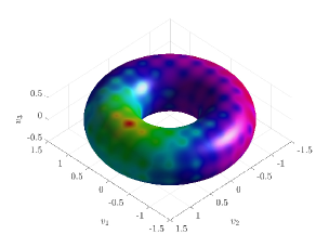
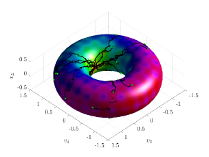
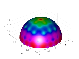
The global minimum is at v=v𝑣subscript𝑣v=v_{*}. In Figure 1 we report in the case d=3𝑑3d=3 the Ackley function constrained over the half sphere v30superscript𝑣30v^{3}\geq 0 and over the torus with external radius R=1𝑅1R=1 and inner radius r=0.5𝑟0.5r=0.5. The colors over the surface represent the values attained by the function.
Refer to caption
Refer to caption
Figure 1: The Ackley function for d=3𝑑3d=3 in the constrained case on two example hypersurfaces. The half sphere SS2superscriptSS2\SS^{2} (left) and the torus with R=1𝑅1R=1 and r=0.5𝑟0.5r=0.5 (right). The global minimum on SS2superscriptSS2\SS^{2} corresponds to the point v=(0,0,1)Tsubscript𝑣superscript001𝑇v_{*}=(0,0,1)^{T}, over the torus to the point v=(0,1,0.5)Tsubscript𝑣superscript010.5𝑇v_{*}=(0,1,0.5)^{T}.
Refer to caption
Refer to caption
Refer to caption
Refer to caption
Refer to caption
Refer to caption
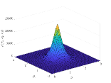
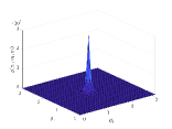
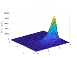
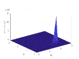
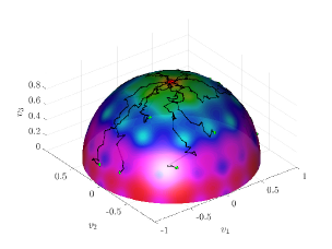
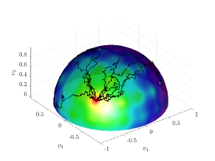
Figure 2: Particles trajectories along the simulation for the Ackley function on the half-sphere in the case d=3𝑑3d=3, N=20𝑁20N=20 with minimum at v=(0,0,1)Tsubscript𝑣superscript001𝑇v_{*}=(0,0,1)^{T} (left) and v=(1/2,1/2,1/2)Tsubscript𝑣superscript121212𝑇v_{*}=(-1/\sqrt{2},-1/2,1/2)^{T} (right). On the top corresponding time evolution of the particle distribution ρ(t,v)𝜌𝑡𝑣\rho(t,v) in angular coordinates at t=1𝑡1t=1 and t=2.5𝑡2.5t=2.5 for N=106𝑁superscript106N=10^{6}. The simulation parameters are Δt=0.05Δ𝑡0.05\Delta t=0.05, σ=0.25𝜎0.25\sigma=0.25 and α=50𝛼50\alpha=50. Although we run the simulation on the entire sphere, we display the result on the half-sphere because, eventually, all particles do converge to one point, hence, all particles do eventually belong to a half sphere (mind that the stochastic process is a time continuous function). Displaying half-sphere is simply aesthetically more pleasing and it allows a better reading of the figures. On the other hand, as soon as one generates initial particles on the half-sphere containing a minimizer, then they - empirically - tend generically to remain on that half sphere, hence there is no need of displaying the rest of the sphere and we do not use any confinement mechanism rather than the given dynamics. Also boundary conditions are actually not imposed.
Refer to caption
Refer to caption
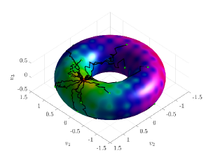
Figure 3: Particles trajectories along the simulation for the Ackley function constrained on the torus with R=1𝑅1R=1 and r=0.5𝑟0.5r=0.5 in the case d=3𝑑3d=3, N=20𝑁20N=20 with minimum at v=(0,1,0.5)Tsubscript𝑣superscript010.5𝑇v_{*}=(0,1,0.5)^{T} (left) and v=(0.5,0,0)Tsubscript𝑣superscript0.500𝑇v_{*}=(0.5,0,0)^{T} (right). The simulation parameters are Δt=0.05Δ𝑡0.05\Delta t=0.05, σ=0.25𝜎0.25\sigma=0.25 and α=50𝛼50\alpha=50.

In the reported simulations we initialize the particles with a uniform distribution over the hypersurface (this typically requires the use of a suitable algorithm, see Ref. [29]) and employ a simple Euler-Maruyama scheme with projection and time step Δt>0Δ𝑡0\Delta t>0. We report in Figure 2 the case of the half-sphere together with the particle trajectories for t[0,5]𝑡05t\in[0,5] with N=20𝑁20N=20, Δt=0.05Δ𝑡0.05\Delta t=0.05, σ=0.25𝜎0.25\sigma=0.25 and α=50𝛼50\alpha=50. On the left we consider the case with minimum at v=(0,0,1)Tsubscript𝑣superscript001𝑇v_{*}=(0,0,1)^{T}, on the right the case with minimum at v=(1/2,1/2,1/2)Tsubscript𝑣superscript121212𝑇v_{*}=(1/\sqrt{2},-1/2,1/2)^{T}. The time evolution of the particle distribution ρ(t,v)𝜌𝑡𝑣\rho(t,v) in the numerical mean field limit for N=106𝑁superscript106N=10^{6} is also reported in the upper part of the same figure.

In Figure 3 we report an analogous simulation in the constrained case on the torus. The numerical parameters are the same as in the previous case. On the left the minimum is located at v=(0,1,0.5)Tsubscript𝑣superscript010.5𝑇v_{*}=(0,1,0.5)^{T}, whereas on the right is located at v=(0.5,0,0)Tsubscript𝑣superscript0.500𝑇v_{*}=(0.5,0,0)^{T}.

As these figures show it, the dynamics consistently converges to the global minimizers totally regardless of the many local minimizers and the large particle system does converges numerically to its mean-field approximation. In the related paper Ref. [29] we rigorously analyze the large time behavior of the system for Γ=𝕊d1Γsuperscript𝕊𝑑1\Gamma=\mathbb{S}^{d-1}, we prove its convergence to global minimizers in a suitable sense, and we provide several applications in machine learning. A proof of convergence to global minimizers for more general hypersurfaces is the subject of current investigation.

Let us conclude this introduction by mentioning that the optimization on the hypersurface offers further numerous advantages, besides allowing a rigorous proof of mean-field limit thanks to the compactness of the hypersurface. First of all a vast class of optimization problems can be reduced to constrained optimizations over hypersurfaces: in a related paper Ref. [29], where we focus on the numerical implementation of the method on the sphere and its asymptotic/convergence analysis to global minimizers, we present also a few relevant and challenging applications in signal processing and machine learning. Due to compactness of the hypersurface, local smoothness and boundedness requirements on \mathcal{E} are necessarily a uniform and global property. However, against these properties that greatly simplify the analysis of the well-posedness of the system and its mean-field limit, the specific topology of the hypersurface may make it harder to prove asymptotic convergence of the dynamics to global miminizers, requiring major technical variations with respect to the approach of unconstrained CBO [13]. We refer to Ref. [29] for the details of the large time analysis of solutions ρ(t,v)𝜌𝑡𝑣\rho(t,v) of (1.7) on the sphere and examples of applications in high-dimension. There we needed to develop ad hoc arguments to prove the asymptotic convergence. A similar consensus dynamics could be in principle defined also on more general compact manifolds [25], but we still lack a general approach to deal with its (global) asymptotic analysis and this research direction needs certainly further investigations.

The rest of the paper is organized as follows: in Section 2 we show that the equations (1.2), (1.7) and (1.8) are well-posed, that is, there is a unique solution for any initial distribution ρ0subscript𝜌0\rho_{0}, which depends continuously on the initial datum, and in Section 3 we address the mean-field limit.

2 Well-posedness

This section focuses on proving the well-posedness for the particle system (1.2), the mean-field dynamic (1.8) and the mean-field PDE (1.7). To ensure this, we make the following smoothness assumption on the objective function \mathcal{E}.

Assumption 2.1.

The objective function 0:d:0superscript𝑑0\leq\mathcal{E}:\mathbb{R}^{d}\rightarrow\mathbb{R} is locally Lipschitz continuous.

2.1 Well-posedness for the interacting particle system (1.2)

Recall that the particle system (1.2) is assumed to evolve in the whole space dsuperscript𝑑\mathbb{R}^{d} instead of on the hypersurface ΓΓ\Gamma directly. We choose this embedding because it provides an explicit and computable representation of the system and it allows for a global description. The difficulty in showing first the well-posedness of (1.2) in the ambient space dsuperscript𝑑\mathbb{R}^{d} is that the projection P(Vti)𝑃superscriptsubscript𝑉𝑡𝑖P(V_{t}^{i}), Δγ(Vti)Δ𝛾superscriptsubscript𝑉𝑡𝑖\Delta\gamma(V_{t}^{i}) and γ(Vti)𝛾superscriptsubscript𝑉𝑡𝑖\nabla\gamma(V_{t}^{i}) may not be well defined when VtiΓ^superscriptsubscript𝑉𝑡𝑖^ΓV_{t}^{i}\notin\widehat{\Gamma}. For example, in the case of the sphere SSd1superscriptSS𝑑1\SS^{d-1}, the projection P(Vti)=IVti(Vti)T|Vti|2𝑃superscriptsubscript𝑉𝑡𝑖𝐼superscriptsubscript𝑉𝑡𝑖superscriptsuperscriptsubscript𝑉𝑡𝑖𝑇superscriptsuperscriptsubscript𝑉𝑡𝑖2P(V_{t}^{i})=I-\frac{V_{t}^{i}(V_{t}^{i})^{T}}{|V_{t}^{i}|^{2}} and Δγ(Vti)γ(Vti)=(d1)Vti|Vti|2Δ𝛾superscriptsubscript𝑉𝑡𝑖𝛾superscriptsubscript𝑉𝑡𝑖𝑑1superscriptsubscript𝑉𝑡𝑖superscriptsuperscriptsubscript𝑉𝑡𝑖2\Delta\gamma(V_{t}^{i})\nabla\gamma(V_{t}^{i})=(d-1)\frac{V_{t}^{i}}{|V_{t}^{i}|^{2}} are not defined for Vti=0superscriptsubscript𝑉𝑡𝑖0V_{t}^{i}=0. In order to overcome this problem, we regularize the diffusion and drift coefficients, that is, we replace them with appropriate functions P1subscript𝑃1P_{1}, P2subscript𝑃2P_{2} and P3subscript𝑃3P_{3} respectively: let P1subscript𝑃1P_{1} be a d×d𝑑𝑑d\times d matrix valued map on dsuperscript𝑑\mathbb{R}^{d} with bounded derivatives such that P1(v)=P(v)subscript𝑃1𝑣𝑃𝑣P_{1}(v)=P(v) for all vΓ^𝑣^Γv\in\widehat{\Gamma}, P2subscript𝑃2P_{2} be a dsuperscript𝑑\mathbb{R}^{d} valued map on \mathbb{R} with bounded derivatives such that P2(v)=Δγ(v)subscript𝑃2𝑣Δ𝛾𝑣P_{2}(v)=\Delta\gamma(v) if vΓ^𝑣^Γv\in\widehat{\Gamma}, and P3subscript𝑃3P_{3} be a dsuperscript𝑑\mathbb{R}^{d} valued map on dsuperscript𝑑\mathbb{R}^{d}, again with bounded derivatives such that P3(v)=γ(v)subscript𝑃3𝑣𝛾𝑣P_{3}(v)=\nabla\gamma(v) if vΓ^𝑣^Γv\in\widehat{\Gamma}. It is also useful to mention that

P(v)γ(v)=0𝑃𝑣𝛾𝑣0P(v)\nabla\gamma(v)=0 (2.1)

and

γ(v)P(v)y=0𝛾𝑣𝑃𝑣𝑦0\nabla\gamma(v)\cdot P(v)y=0 (2.2)

hold for any yd𝑦superscript𝑑y\in\mathbb{R}^{d}. For later use, let us denote [N]={1,,N}delimited-[]𝑁1𝑁[N]=\{1,\dots,N\}. Additionally, we regularize the locally Lipschitz function \mathcal{E}: Let us introduce ~(v)~𝑣\tilde{\mathcal{E}}(v) satisfying the following assumptions

Assumption 2.2.

The regularized extension function ~:d:~superscript𝑑\tilde{\mathcal{E}}:\mathbb{R}^{d}\rightarrow\mathbb{R} is globally Lipschitz continuous and satisfies the properties

  • 1.

    ~(v)=(v)~𝑣𝑣\tilde{\mathcal{E}}(v)=\mathcal{E}(v) when vΓ^𝑣^Γv\in\widehat{\Gamma};

  • 2.

    ~(v)~(u)L|vu|~𝑣~𝑢𝐿𝑣𝑢\tilde{\mathcal{E}}(v)-\tilde{\mathcal{E}}(u)\leq L|v-u| for all u,vd𝑢𝑣superscript𝑑u,v\in\mathbb{R}^{d} for a suitable global Lipschitz constant L>0𝐿0L>0;

  • 3.

    <¯~:=inf~~sup~=:~¯<+-\infty<\underline{\tilde{\mathcal{E}}}:=\inf\tilde{\mathcal{E}}\leq\tilde{\mathcal{E}}\leq\sup\tilde{\mathcal{E}}=:\overline{\tilde{\mathcal{E}}}<+\infty .

Remark 2.1.

Here ~~\tilde{\mathcal{E}} is introduced as an auxiliary function for the proof of well-posedness and mean-field limit only, and it does not play any role in actual optimization problem, which is defined on ΓΓ\Gamma. Indeed, as we can see in Theorem 2.1 below, particles stay on the hypersurface ΓΓ\Gamma all the time, which means that certainly vΓ^𝑣^Γv\in\widehat{\Gamma}, so one has ~(v)(v)~𝑣𝑣\tilde{\mathcal{E}}(v)\equiv\mathcal{E}(v).

We note here that \mathcal{E} and ~~\tilde{\mathcal{E}} appearing the sequel always satisfy Assumptions 2.1 and 2.2. Given such P1subscript𝑃1P_{1}, P2subscript𝑃2P_{2}, P3subscript𝑃3P_{3} and ~~\tilde{\mathcal{E}}, we introduce the following regularized particle system

dVti𝑑superscriptsubscript𝑉𝑡𝑖\displaystyle dV_{t}^{i} =λP1(Vti)(Vtivα,~(ρtN))dt+σ|Vtivα,~(ρtN)|P1(Vti)dBtiσ22(Vtivα,~(ρtN))2P2(Vti)P3(Vti)dt,absent𝜆subscript𝑃1superscriptsubscript𝑉𝑡𝑖superscriptsubscript𝑉𝑡𝑖subscript𝑣𝛼~superscriptsubscript𝜌𝑡𝑁𝑑𝑡𝜎superscriptsubscript𝑉𝑡𝑖subscript𝑣𝛼~superscriptsubscript𝜌𝑡𝑁subscript𝑃1superscriptsubscript𝑉𝑡𝑖𝑑superscriptsubscript𝐵𝑡𝑖superscript𝜎22superscriptsuperscriptsubscript𝑉𝑡𝑖subscript𝑣𝛼~superscriptsubscript𝜌𝑡𝑁2subscript𝑃2superscriptsubscript𝑉𝑡𝑖subscript𝑃3superscriptsubscript𝑉𝑡𝑖𝑑𝑡\displaystyle=-\lambda P_{1}(V_{t}^{i})(V_{t}^{i}-v_{\alpha,\tilde{\mathcal{E}}}(\rho_{t}^{N}))dt+\sigma|V_{t}^{i}-v_{\alpha,\tilde{\mathcal{E}}}(\rho_{t}^{N})|P_{1}(V_{t}^{i})dB_{t}^{i}-\frac{\sigma^{2}}{2}(V_{t}^{i}-v_{\alpha,\tilde{\mathcal{E}}}(\rho_{t}^{N}))^{2}P_{2}(V_{t}^{i})P_{3}(V_{t}^{i})dt\,, (2.3)

for i[N]𝑖delimited-[]𝑁i\in[N], where

vα,~(ρtN)=dvωα~(v)𝑑ρtNdωα~(v)𝑑ρtN,ωα~(v)=eα~(v).formulae-sequencesubscript𝑣𝛼~superscriptsubscript𝜌𝑡𝑁subscriptsuperscript𝑑𝑣superscriptsubscript𝜔𝛼~𝑣differential-dsuperscriptsubscript𝜌𝑡𝑁subscriptsuperscript𝑑superscriptsubscript𝜔𝛼~𝑣differential-dsuperscriptsubscript𝜌𝑡𝑁superscriptsubscript𝜔𝛼~𝑣superscript𝑒𝛼~𝑣v_{\alpha,\tilde{\mathcal{E}}}(\rho_{t}^{N})=\frac{\int_{\mathbb{R}^{d}}v\omega_{\alpha}^{\tilde{\mathcal{E}}}(v)d\rho_{t}^{N}}{\int_{\mathbb{R}^{d}}\omega_{\alpha}^{\tilde{\mathcal{E}}}(v)d\rho_{t}^{N}}\,,\qquad\omega_{\alpha}^{\tilde{\mathcal{E}}}(v)=e^{-\alpha{\tilde{\mathcal{E}}}(v)}\,. (2.4)

Next we can deduce that the coefficients in (2.3) are locally Lipschitz continuous and have linear growth. More precisely, we have the following result.

Lemma 2.1.

Let N𝑁N\in\mathbb{N}, α>0𝛼0\alpha>0 be arbitrary and ~~\tilde{\mathcal{E}} satisfy Assumption 2.2. Then for any 𝐕N,𝐕^NNdsuperscript𝐕𝑁superscript^𝐕𝑁superscript𝑁𝑑\mathbf{V}^{N},\widehat{\mathbf{V}}^{N}\in\mathbb{R}^{Nd}, and corresponding empirical measures ρN=1Ni=1NδVi,superscript𝜌𝑁1𝑁superscriptsubscript𝑖1𝑁subscript𝛿superscript𝑉𝑖\rho^{N}=\frac{1}{N}\sum_{i=1}^{N}\delta_{V^{i}}\,, and ρ^N=1Ni=1NδV^i,superscript^𝜌𝑁1𝑁superscriptsubscript𝑖1𝑁subscript𝛿superscript^𝑉𝑖\widehat{\rho}^{N}=\frac{1}{N}\sum_{i=1}^{N}\delta_{\widehat{V}^{i}}\,, it holds

|vα,~(ρN)|1NCα,~𝐕N1subscript𝑣𝛼~superscript𝜌𝑁1𝑁subscript𝐶𝛼~subscriptnormsuperscript𝐕𝑁1|v_{\alpha,\tilde{\mathcal{E}}}(\rho^{N})|\leq\frac{1}{N}C_{\alpha,\tilde{\mathcal{E}}}\|\mathbf{V}^{N}\|_{1} (2.5)

and

|vα,~(ρ^N)vα,~(ρN)|(Cα,~N+2αLCα,~N𝐕^N)𝐕N𝐕^N1,subscript𝑣𝛼~superscript^𝜌𝑁subscript𝑣𝛼~superscript𝜌𝑁subscript𝐶𝛼~𝑁2𝛼𝐿subscript𝐶𝛼~𝑁subscriptnormsuperscript^𝐕𝑁subscriptnormsuperscript𝐕𝑁superscript^𝐕𝑁1|v_{\alpha,\tilde{\mathcal{E}}}(\widehat{\rho}^{N})-v_{\alpha,\tilde{\mathcal{E}}}(\rho^{N})|\leq\left(\frac{C_{\alpha,\tilde{\mathcal{E}}}}{N}+\frac{2\alpha LC_{\alpha,\tilde{\mathcal{E}}}}{N}\|\mathbf{\widehat{V}}^{N}\|_{\infty}\right)\|\mathbf{V}^{N}-\mathbf{\widehat{V}}^{N}\|_{1}\,, (2.6)

where Cα,~=eα(~¯¯~)subscript𝐶𝛼~superscript𝑒𝛼¯~¯~C_{\alpha,\tilde{\mathcal{E}}}=e^{\alpha(\overline{\tilde{\mathcal{E}}}-\underline{\tilde{\mathcal{E}}})}. Here we used the notations for norms of vectors 𝐕=supi[N]|Vi|subscriptnorm𝐕subscriptsupremum𝑖delimited-[]𝑁superscript𝑉𝑖\|\mathbf{V}\|_{\infty}=\sup_{i\in[N]}|V^{i}| and 𝐕1=i=1N|Vi|subscriptnorm𝐕1superscriptsubscript𝑖1𝑁superscript𝑉𝑖\|\mathbf{V}\|_{1}=\sum_{i=1}^{N}|V^{i}|.

Proof.

First, one notes that

eα~¯ωα~(Vj)=eα~(Vj)eα¯~.superscript𝑒𝛼¯~superscriptsubscript𝜔𝛼~superscript𝑉𝑗superscript𝑒𝛼~superscript𝑉𝑗superscript𝑒𝛼¯~e^{-\alpha\overline{\tilde{\mathcal{E}}}}\leq\omega_{\alpha}^{\tilde{\mathcal{E}}}(V^{j})=e^{-\alpha\tilde{\mathcal{E}}(V^{j})}\leq e^{-\alpha\underline{\tilde{\mathcal{E}}}}\,. (2.7)

Then we have

|vα,~(ρN)|=|j=1NVjeα~(Vj)j=1Neα~(Vj)|1Neα(~¯¯~)j=1N|Vj|=1NCα,~𝐕N1,subscript𝑣𝛼~superscript𝜌𝑁superscriptsubscript𝑗1𝑁superscript𝑉𝑗superscript𝑒𝛼~superscript𝑉𝑗superscriptsubscript𝑗1𝑁superscript𝑒𝛼~superscript𝑉𝑗1𝑁superscript𝑒𝛼¯~¯~superscriptsubscript𝑗1𝑁superscript𝑉𝑗1𝑁subscript𝐶𝛼~subscriptnormsuperscript𝐕𝑁1\displaystyle|v_{\alpha,\tilde{\mathcal{E}}}(\rho^{N})|=\left|\frac{\sum_{j=1}^{N}V^{j}e^{-\alpha\tilde{\mathcal{E}}(V^{j})}}{\sum_{j=1}^{N}e^{-\alpha\tilde{\mathcal{E}}(V^{j})}}\right|\leq\frac{1}{N}e^{\alpha(\overline{\tilde{\mathcal{E}}}-\underline{\tilde{\mathcal{E}}})}\sum_{j=1}^{N}|V^{j}|=\frac{1}{N}C_{\alpha,\tilde{\mathcal{E}}}\|\mathbf{V}^{N}\|_{1}\,,

where Cα,~:=eα(~¯¯~)assignsubscript𝐶𝛼~superscript𝑒𝛼¯~¯~C_{\alpha,\tilde{\mathcal{E}}}:=e^{\alpha(\overline{\tilde{\mathcal{E}}}-\underline{\tilde{\mathcal{E}}})}. Next we split the error

vα,~(ρ^N)vα,~(ρN)subscript𝑣𝛼~superscript^𝜌𝑁subscript𝑣𝛼~superscript𝜌𝑁\displaystyle v_{\alpha,\tilde{\mathcal{E}}}(\widehat{\rho}^{N})-v_{\alpha,\tilde{\mathcal{E}}}(\rho^{N}) =j=1N(VjV^j)ωα~(Vj)j=1Nωα~(Vj)+j=1NV^j(ωα~(Vj)ωα~(V^j))j=1Nωα~(Vj)absentsuperscriptsubscript𝑗1𝑁superscript𝑉𝑗superscript^𝑉𝑗superscriptsubscript𝜔𝛼~superscript𝑉𝑗superscriptsubscript𝑗1𝑁superscriptsubscript𝜔𝛼~superscript𝑉𝑗superscriptsubscript𝑗1𝑁superscript^𝑉𝑗superscriptsubscript𝜔𝛼~superscript𝑉𝑗superscriptsubscript𝜔𝛼~superscript^𝑉𝑗superscriptsubscript𝑗1𝑁superscriptsubscript𝜔𝛼~superscript𝑉𝑗\displaystyle=\frac{\sum_{j=1}^{N}(V^{j}-\widehat{V}^{j})\omega_{\alpha}^{\tilde{\mathcal{E}}}(V^{j})}{\sum_{j=1}^{N}\omega_{\alpha}^{\tilde{\mathcal{E}}}(V^{j})}+\frac{\sum_{j=1}^{N}\widehat{V}^{j}(\omega_{\alpha}^{\tilde{\mathcal{E}}}(V^{j})-\omega_{\alpha}^{\tilde{\mathcal{E}}}(\widehat{V}^{j}))}{\sum_{j=1}^{N}\omega_{\alpha}^{\tilde{\mathcal{E}}}(V^{j})}
+j=1NV^jωα~(V^j)j=1N(ωα~(V^j)ωα~(Vj))(j=1Nωα~(Vj))(j=1Nωα~(V^j))superscriptsubscript𝑗1𝑁superscript^𝑉𝑗superscriptsubscript𝜔𝛼~superscript^𝑉𝑗superscriptsubscript𝑗1𝑁superscriptsubscript𝜔𝛼~superscript^𝑉𝑗superscriptsubscript𝜔𝛼~superscript𝑉𝑗superscriptsubscript𝑗1𝑁superscriptsubscript𝜔𝛼~superscript𝑉𝑗superscriptsubscript𝑗1𝑁superscriptsubscript𝜔𝛼~superscript^𝑉𝑗\displaystyle\quad+\frac{\sum_{j=1}^{N}\widehat{V}^{j}\omega_{\alpha}^{\tilde{\mathcal{E}}}(\widehat{V}^{j})\sum_{j=1}^{N}(\omega_{\alpha}^{\tilde{\mathcal{E}}}(\widehat{V}^{j})-\omega_{\alpha}^{\tilde{\mathcal{E}}}(V^{j}))}{(\sum_{j=1}^{N}\omega_{\alpha}^{\tilde{\mathcal{E}}}(V^{j}))(\sum_{j=1}^{N}\omega_{\alpha}^{\tilde{\mathcal{E}}}(\widehat{V}^{j}))}
=:I1+I2+I3.\displaystyle=:I_{1}+I_{2}+I_{3}\,. (2.8)

For I1subscript𝐼1I_{1}, the previous computation yields

|I1|1NCα,~𝐕N𝐕^N1,subscript𝐼11𝑁subscript𝐶𝛼~subscriptnormsuperscript𝐕𝑁superscript^𝐕𝑁1|I_{1}|\leq\frac{1}{N}C_{\alpha,\tilde{\mathcal{E}}}\|\mathbf{V}^{N}-\mathbf{\widehat{V}}^{N}\|_{1}\,, (2.9)

Notice that it holds

|ωα~(Vj)ωα~(V^j)|=|eα~(Vj)eα~(V^j)|αeα¯~|~(Vj)~(V^j)|αLeα¯~|VjV^j|.superscriptsubscript𝜔𝛼~superscript𝑉𝑗superscriptsubscript𝜔𝛼~superscript^𝑉𝑗superscript𝑒𝛼~superscript𝑉𝑗superscript𝑒𝛼~superscript^𝑉𝑗𝛼superscript𝑒𝛼¯~~superscript𝑉𝑗~superscript^𝑉𝑗𝛼𝐿superscript𝑒𝛼¯~superscript𝑉𝑗superscript^𝑉𝑗\displaystyle|\omega_{\alpha}^{\tilde{\mathcal{E}}}(V^{j})-\omega_{\alpha}^{\tilde{\mathcal{E}}}(\widehat{V}^{j})|=|e^{-\alpha\tilde{\mathcal{E}}(V^{j})}-e^{-\alpha\tilde{\mathcal{E}}(\widehat{V}^{j})}|\leq\alpha e^{-\alpha\underline{\tilde{\mathcal{E}}}}|\tilde{\mathcal{E}}(V^{j})-\tilde{\mathcal{E}}(\widehat{V}^{j})|\leq\alpha Le^{-\alpha\underline{\tilde{\mathcal{E}}}}|V^{j}-\widehat{V}^{j}|\,.

Thus we conclude that

max{|I2|,|I3|}αLCα,~N𝐕^N𝐕N𝐕^N1.subscript𝐼2subscript𝐼3𝛼𝐿subscript𝐶𝛼~𝑁subscriptnormsuperscript^𝐕𝑁subscriptnormsuperscript𝐕𝑁superscript^𝐕𝑁1\max\{|I_{2}|\,,|I_{3}|\}\leq\frac{\alpha LC_{\alpha,\tilde{\mathcal{E}}}}{N}\|\mathbf{\widehat{V}}^{N}\|_{\infty}\|\mathbf{V}^{N}-\mathbf{\widehat{V}}^{N}\|_{1}\,. (2.10)

Collecting estimates (2.9) and (2.10) completes the proof. ∎

Theorem 2.1.

Under Assumptions 2.1 and 2.2 let ρ0subscript𝜌0\rho_{0} be a probability measure on ΓΓ\Gamma and, for every N𝑁N\in\mathbb{N}, (V0i)i[N]subscriptsuperscriptsubscript𝑉0𝑖𝑖delimited-[]𝑁(V_{0}^{i})_{i\in[N]} be N𝑁N i.i.d. random variables with the common law ρ0subscript𝜌0\rho_{0}. For every N𝑁N\in\mathbb{N}, there exists a pathwise unique strong solution ((Vti)t0)i[N]subscriptsubscriptsuperscriptsubscript𝑉𝑡𝑖𝑡0𝑖delimited-[]𝑁((V_{t}^{i})_{t\geq 0})_{i\in[N]} to the particle system (1.2) with the initial data (V0i)i[N]subscriptsuperscriptsubscript𝑉0𝑖𝑖delimited-[]𝑁(V_{0}^{i})_{i\in[N]}. Moreover it holds that VtiΓsuperscriptsubscript𝑉𝑡𝑖ΓV_{t}^{i}\in\Gamma for all i[N]𝑖delimited-[]𝑁i\in[N] and any t>0𝑡0t>0.

Proof.

Given P1subscript𝑃1P_{1}, P2subscript𝑃2P_{2}, P3subscript𝑃3P_{3} and ~~\tilde{\mathcal{E}}, the SDE (2.3) has locally Lipschitz coefficients, so it admits a pathwise unique local strong solution by standard SDE well-posedness result [24, Chap. 5, Theorem 3.1]. Moreover, it follows from Itô’s formula (5.1) (choosing φ(x)=γ(x)𝜑𝑥𝛾𝑥\varphi(x)=\gamma(x)), as long as VtiΓ^superscriptsubscript𝑉𝑡𝑖^ΓV_{t}^{i}\in\widehat{\Gamma} (the process is continuous and we can nevertheless consider a smooth extension of γ𝛾\gamma out of Γ^^Γ\widehat{\Gamma}), that

dγ(Vti)𝑑𝛾superscriptsubscript𝑉𝑡𝑖\displaystyle d\gamma(V_{t}^{i}) =λγ(Vti)P(Vti)(Vtivα,~(ρtN))dt+σ|Vtivα,~(ρtN)|γ(Vti)P(Vti)dBtiabsent𝜆𝛾superscriptsubscript𝑉𝑡𝑖𝑃superscriptsubscript𝑉𝑡𝑖superscriptsubscript𝑉𝑡𝑖subscript𝑣𝛼~superscriptsubscript𝜌𝑡𝑁𝑑𝑡𝜎superscriptsubscript𝑉𝑡𝑖subscript𝑣𝛼~superscriptsubscript𝜌𝑡𝑁𝛾superscriptsubscript𝑉𝑡𝑖𝑃superscriptsubscript𝑉𝑡𝑖𝑑superscriptsubscript𝐵𝑡𝑖\displaystyle=-\lambda\nabla\gamma(V_{t}^{i})\cdot P(V_{t}^{i})(V_{t}^{i}-v_{\alpha,\tilde{\mathcal{E}}}(\rho_{t}^{N}))dt+\sigma|V_{t}^{i}-v_{\alpha,\tilde{\mathcal{E}}}(\rho_{t}^{N})|\nabla\gamma(V_{t}^{i})\cdot P(V_{t}^{i})dB_{t}^{i}
12σ2(Vtivα,~(ρtN))2Δγ(Vti)dt12superscript𝜎2superscriptsuperscriptsubscript𝑉𝑡𝑖subscript𝑣𝛼~superscriptsubscript𝜌𝑡𝑁2Δ𝛾superscriptsubscript𝑉𝑡𝑖𝑑𝑡\displaystyle\quad-\frac{1}{2}\sigma^{2}(V_{t}^{i}-v_{\alpha,\tilde{\mathcal{E}}}(\rho_{t}^{N}))^{2}\Delta\gamma(V_{t}^{i})dt
+12σ2(Vtivα,~(ρtN))2k,=1dk,2γ(Vti)(ekTkγ(Vti)γ(Vti)T)(eγ(Vti)γ(Vti))dt12superscript𝜎2superscriptsuperscriptsubscript𝑉𝑡𝑖subscript𝑣𝛼~superscriptsubscript𝜌𝑡𝑁2superscriptsubscript𝑘1𝑑superscriptsubscript𝑘2𝛾superscriptsubscript𝑉𝑡𝑖superscriptsubscript𝑒𝑘𝑇subscript𝑘𝛾superscriptsubscript𝑉𝑡𝑖𝛾superscriptsuperscriptsubscript𝑉𝑡𝑖𝑇subscript𝑒subscript𝛾superscriptsubscript𝑉𝑡𝑖𝛾superscriptsubscript𝑉𝑡𝑖𝑑𝑡\displaystyle\quad+\frac{1}{2}\sigma^{2}(V_{t}^{i}-v_{\alpha,\tilde{\mathcal{E}}}(\rho_{t}^{N}))^{2}\sum_{k,\ell=1}^{d}\partial_{k,\ell}^{2}\gamma(V_{t}^{i})\left(e_{k}^{T}-\partial_{k}\gamma(V_{t}^{i})\nabla\gamma(V_{t}^{i})^{T}\right)\left(e_{\ell}-\partial_{\ell}\gamma(V_{t}^{i})\nabla\gamma(V_{t}^{i})\right)dt
=12σ2(Vtivα,~(ρtN))2Δγ(Vti)dt+12σ2(Vtivα,~(ρtN))2kdk2γ(Vti)dtabsent12superscript𝜎2superscriptsuperscriptsubscript𝑉𝑡𝑖subscript𝑣𝛼~superscriptsubscript𝜌𝑡𝑁2Δ𝛾superscriptsubscript𝑉𝑡𝑖𝑑𝑡12superscript𝜎2superscriptsuperscriptsubscript𝑉𝑡𝑖subscript𝑣𝛼~superscriptsubscript𝜌𝑡𝑁2superscriptsubscript𝑘𝑑superscriptsubscript𝑘2𝛾superscriptsubscript𝑉𝑡𝑖𝑑𝑡\displaystyle=-\frac{1}{2}\sigma^{2}(V_{t}^{i}-v_{\alpha,\tilde{\mathcal{E}}}(\rho_{t}^{N}))^{2}\Delta\gamma(V_{t}^{i})dt+\frac{1}{2}\sigma^{2}(V_{t}^{i}-v_{\alpha,\tilde{\mathcal{E}}}(\rho_{t}^{N}))^{2}\sum_{k}^{d}\partial_{k}^{2}\gamma(V_{t}^{i})dt
+12σ2(Vtivα,~(ρtN))2(k,=1dk,2γ(Vti)kγ(Vti)γ(Vti))dt12superscript𝜎2superscriptsuperscriptsubscript𝑉𝑡𝑖subscript𝑣𝛼~superscriptsubscript𝜌𝑡𝑁2superscriptsubscript𝑘1𝑑superscriptsubscript𝑘2𝛾superscriptsubscript𝑉𝑡𝑖subscript𝑘𝛾superscriptsubscript𝑉𝑡𝑖subscript𝛾superscriptsubscript𝑉𝑡𝑖𝑑𝑡\displaystyle\quad+\frac{1}{2}\sigma^{2}(V_{t}^{i}-v_{\alpha,\tilde{\mathcal{E}}}(\rho_{t}^{N}))^{2}\left(-\sum_{k,\ell=1}^{d}\partial_{k,\ell}^{2}\gamma(V_{t}^{i})\partial_{k}\gamma(V_{t}^{i})\partial_{\ell}\gamma(V_{t}^{i})\right)dt
=12σ2(Vtivα,~(ρtN))2Δγ(Vti)dt+12σ2(Vtivα,~(ρtN))2Δγ(Vti)dtabsent12superscript𝜎2superscriptsuperscriptsubscript𝑉𝑡𝑖subscript𝑣𝛼~superscriptsubscript𝜌𝑡𝑁2Δ𝛾superscriptsubscript𝑉𝑡𝑖𝑑𝑡12superscript𝜎2superscriptsuperscriptsubscript𝑉𝑡𝑖subscript𝑣𝛼~superscriptsubscript𝜌𝑡𝑁2Δ𝛾superscriptsubscript𝑉𝑡𝑖𝑑𝑡\displaystyle=-\frac{1}{2}\sigma^{2}(V_{t}^{i}-v_{\alpha,\tilde{\mathcal{E}}}(\rho_{t}^{N}))^{2}\Delta\gamma(V_{t}^{i})dt+\frac{1}{2}\sigma^{2}(V_{t}^{i}-v_{\alpha,\tilde{\mathcal{E}}}(\rho_{t}^{N}))^{2}\Delta\gamma(V_{t}^{i})dt
+12σ2(Vtivα,~(ρtN))2(12d|γ(Vti)|2γ(Vti))dt( since |γ|=1)12superscript𝜎2superscriptsuperscriptsubscript𝑉𝑡𝑖subscript𝑣𝛼~superscriptsubscript𝜌𝑡𝑁212superscriptsubscript𝑑subscriptsuperscript𝛾superscriptsubscript𝑉𝑡𝑖2subscript𝛾superscriptsubscript𝑉𝑡𝑖𝑑𝑡 since 𝛾1\displaystyle\quad+\frac{1}{2}\sigma^{2}(V_{t}^{i}-v_{\alpha,\tilde{\mathcal{E}}}(\rho_{t}^{N}))^{2}\left(-\frac{1}{2}\sum_{\ell}^{d}\partial_{\ell}|\nabla\gamma(V_{t}^{i})|^{2}\partial_{\ell}\gamma(V_{t}^{i})\right)dt\quad(\mbox{ since }|\nabla\gamma|=1)
=0,absent0\displaystyle=0\,, (2.11)

where kγ(Vti)subscript𝑘𝛾superscriptsubscript𝑉𝑡𝑖\partial_{k}\gamma(V_{t}^{i}) is the k𝑘k-th component of γ(Vti)𝛾superscriptsubscript𝑉𝑡𝑖\nabla\gamma(V_{t}^{i}), eksubscript𝑒𝑘e_{k} is the unit vector along the k𝑘kth dimension, and we have used the property of P(Vti)𝑃superscriptsubscript𝑉𝑡𝑖P(V_{t}^{i}) as in (2.2). Hence γ(Vti)=γ(V0i)=0𝛾superscriptsubscript𝑉𝑡𝑖𝛾superscriptsubscript𝑉0𝑖0\gamma(V_{t}^{i})=\gamma(V_{0}^{i})=0 for all t>0𝑡0t>0, which ensures that the solution keeps bounded at finite time, hence we have a global solution. Since all VtiΓsuperscriptsubscript𝑉𝑡𝑖ΓV_{t}^{i}\in\Gamma, the solution to the regularized system (2.3) is a solution to (1.2), which provides the global existence of solutions to (1.2).

To show pathwise uniqueness let us consider two solutions to (1.2) for the same initial distribution and Brownian motion. According to the above computation these two solutions stay on the hypersurface for any t0𝑡0t\geq 0, hence they are solutions to the regularized system (2.3), whose solutions are pathwise unique due to the locally Lipschitz continuous coefficients. Hence we have uniqueness for solutions to (1.2). ∎

2.2 Well-posedness for the mean-field dynamic (1.8)

For readers’ convenience, we give a brief introduction of the Wasserstein metric in the following definition, we refer to Ref. [5] for more details.

Definition 2.1 (Wasserstein Metric).

Let 1p<1𝑝1\leq p<\infty and 𝒫p(d)subscript𝒫𝑝superscript𝑑\mathcal{P}_{p}(\mathbb{R}^{d}) be the space of Borel probability measures on dsuperscript𝑑\mathbb{R}^{d} with finite p𝑝p-moment. We equip this space with the Wasserstein distance

Wpp(μ,ν):=inf{d×d|zz^|p𝑑π(μ,ν)|πΠ(μ,ν)}assignsuperscriptsubscript𝑊𝑝𝑝𝜇𝜈infimumconditionalsubscriptsuperscript𝑑superscript𝑑superscript𝑧^𝑧𝑝differential-d𝜋𝜇𝜈𝜋Π𝜇𝜈W_{p}^{p}(\mu,\nu):=\inf\left\{\int_{\mathbb{R}^{d}\times\mathbb{R}^{d}}|z-\hat{z}|^{p}\ d\pi(\mu,\nu)\ \big{|}\ \pi\in\Pi(\mu,\nu)\right\} (2.12)

where Π(μ,ν)Π𝜇𝜈\Pi(\mu,\nu) denotes the collection of all Borel probability measures on d×dsuperscript𝑑superscript𝑑\mathbb{R}^{d}\times\mathbb{R}^{d} with marginals μ𝜇\mu and ν𝜈\nu in the first and second component respectively. The Wasserstein distance can also be expressed as

Wpp(μ,ν)=inf{𝔼[|ZZ¯|p]}superscriptsubscript𝑊𝑝𝑝𝜇𝜈infimum𝔼delimited-[]superscript𝑍¯𝑍𝑝W_{p}^{p}(\mu,\nu)=\inf\left\{\mathbb{E}[|Z-\overline{Z}|^{p}]\right\} (2.13)

where the infimum is taken over all joint distributions of the random variables Z𝑍Z, Z¯¯𝑍\overline{Z} with marginals μ𝜇\mu, ν𝜈\nu respectively.

Notice now that, for any ρ𝒫1(d)𝜌subscript𝒫1superscript𝑑\rho\in\mathcal{P}_{1}(\mathbb{R}^{d})

eα¯~eα~L1(ρ)eα(~¯¯~)=:Cα,~.\displaystyle\frac{e^{-\alpha\underline{\tilde{\mathcal{E}}}}}{\|{e^{-\alpha\tilde{\mathcal{E}}}}\|_{L^{1}(\rho)}}\leq e^{\alpha(\overline{\tilde{\mathcal{E}}}-\underline{\tilde{\mathcal{E}}})}=:C_{\alpha,\tilde{\mathcal{E}}}\,. (2.14)

A direct application of above leads to

|vα,~(ρ)|:=|dvωα~(v)𝑑ρdωα~(v)𝑑ρ|=|dveα~(v)𝑑ρeα~L1(ρ)|Cα,~d|v|𝑑ρ.assignsubscript𝑣𝛼~𝜌subscriptsuperscript𝑑𝑣superscriptsubscript𝜔𝛼~𝑣differential-d𝜌subscriptsuperscript𝑑superscriptsubscript𝜔𝛼~𝑣differential-d𝜌subscriptsuperscript𝑑𝑣superscript𝑒𝛼~𝑣differential-d𝜌subscriptnormsuperscript𝑒𝛼~superscript𝐿1𝜌subscript𝐶𝛼~subscriptsuperscript𝑑𝑣differential-d𝜌|v_{\alpha,\tilde{\mathcal{E}}}(\rho)|:=\left|\frac{\int_{\mathbb{R}^{d}}v\omega_{\alpha}^{\tilde{\mathcal{E}}}(v)\,d\rho}{\int_{\mathbb{R}^{d}}\omega_{\alpha}^{\tilde{\mathcal{E}}}(v)\,d\rho}\right|=\left|\frac{\int_{\mathbb{R}^{d}}ve^{-\alpha\tilde{\mathcal{E}}(v)}\,d\rho}{\|{e^{-\alpha\tilde{\mathcal{E}}}}\|_{L^{1}(\rho)}}\right|\leq C_{\alpha,\tilde{\mathcal{E}}}\int_{\mathbb{R}^{d}}|v|d\rho\,. (2.15)
Lemma 2.2.

Assume that ρ,ρ^𝒫c(d)𝜌^𝜌subscript𝒫𝑐superscript𝑑\rho,\widehat{\rho}\in\mathcal{P}_{c}(\mathbb{R}^{d}) (with compact support), then the following stability estimate holds

|vα,~(ρ)vα,~(ρ^)|CWp(ρ,ρ^),subscript𝑣𝛼~𝜌subscript𝑣𝛼~^𝜌𝐶subscript𝑊𝑝𝜌^𝜌|v_{\alpha,\tilde{\mathcal{E}}}(\rho)-v_{\alpha,\tilde{\mathcal{E}}}(\widehat{\rho})|\leq CW_{p}(\rho,\widehat{\rho})\,, (2.16)

for any 1p<1𝑝1\leq p<\infty, where C=C(Cα,~,α,L)>0𝐶𝐶subscript𝐶𝛼~𝛼𝐿0C=C(C_{\alpha,\tilde{\mathcal{E}}},\alpha,L)>0.

Proof.

Let us compute the difference

vα,~(ρ)vα,~(ρ^)subscript𝑣𝛼~𝜌subscript𝑣𝛼~^𝜌\displaystyle v_{\alpha,\tilde{\mathcal{E}}}(\rho)-v_{\alpha,\tilde{\mathcal{E}}}(\widehat{\rho}) =dveα~(v)𝑑ρ(v)eα~L1(ρ)dv^eα~(v^)𝑑ρ^(v^)eα~L1(ρ^)absentsubscriptsuperscript𝑑𝑣superscript𝑒𝛼~𝑣differential-d𝜌𝑣subscriptnormsuperscript𝑒𝛼~superscript𝐿1𝜌subscriptsuperscript𝑑^𝑣superscript𝑒𝛼~^𝑣differential-d^𝜌^𝑣subscriptnormsuperscript𝑒𝛼~superscript𝐿1^𝜌\displaystyle=\frac{\int_{\mathbb{R}^{d}}ve^{-\alpha\tilde{\mathcal{E}}(v)}\,d\rho(v)}{\|{e^{-\alpha\tilde{\mathcal{E}}}}\|_{L^{1}(\rho)}}-\frac{\int_{\mathbb{R}^{d}}\widehat{v}e^{-\alpha\tilde{\mathcal{E}}(\widehat{v})}\,d\widehat{\rho}(\widehat{v})}{\|{e^{-\alpha\tilde{\mathcal{E}}}}\|_{L^{1}(\widehat{\rho})}}
=d×dveα~(v)eα~L1(ρ)v^eα~(v^)eα~L1(ρ^):=h(v)h(v^)𝑑π(v,v^)absentsubscriptdouble-integralsuperscript𝑑superscript𝑑subscript𝑣superscript𝑒𝛼~𝑣subscriptnormsuperscript𝑒𝛼~superscript𝐿1𝜌^𝑣superscript𝑒𝛼~^𝑣subscriptnormsuperscript𝑒𝛼~superscript𝐿1^𝜌assignabsent𝑣^𝑣differential-d𝜋𝑣^𝑣\displaystyle=\iint_{\mathbb{R}^{d}\times\mathbb{R}^{d}}\underbrace{\frac{ve^{-\alpha\tilde{\mathcal{E}}(v)}}{\|{e^{-\alpha\tilde{\mathcal{E}}}}\|_{L^{1}(\rho)}}-\frac{\widehat{v}e^{-\alpha\tilde{\mathcal{E}}(\widehat{v})}}{\|{e^{-\alpha\tilde{\mathcal{E}}}}\|_{L^{1}(\widehat{\rho})}}}_{:=h(v)-h(\widehat{v})}d\pi(v,\widehat{v})

where πΠ(ρ,ρ^)𝜋Π𝜌^𝜌\pi\in\Pi(\rho,\widehat{\rho}) is an arbitrary coupling of ρ𝜌\rho and ρ^^𝜌\widehat{\rho}. We can write the integrand as follows

h(v)h(v^)𝑣^𝑣\displaystyle h(v)-h(\widehat{v}) =(vv^)eα~(v^)eα~L1(ρ)=:I1+v^(eα~(v)eα~(v^))eα~L1(ρ)=:I2+v^eα~(v^)eα~L1(ρ)v^eα~(v^)eα~L1(ρ^):=I3absentsubscript𝑣^𝑣superscript𝑒𝛼~^𝑣subscriptnormsuperscript𝑒𝛼~superscript𝐿1𝜌:absentsubscript𝐼1subscript^𝑣superscript𝑒𝛼~𝑣superscript𝑒𝛼~^𝑣subscriptnormsuperscript𝑒𝛼~superscript𝐿1𝜌:absentsubscript𝐼2subscript^𝑣superscript𝑒𝛼~^𝑣subscriptnormsuperscript𝑒𝛼~superscript𝐿1𝜌^𝑣superscript𝑒𝛼~^𝑣subscriptnormsuperscript𝑒𝛼~superscript𝐿1^𝜌assignabsentsubscript𝐼3\displaystyle=\underbrace{\frac{(v-\widehat{v})e^{-\alpha\tilde{\mathcal{E}}(\widehat{v})}}{\|{e^{-\alpha\tilde{\mathcal{E}}}}\|_{L^{1}(\rho)}}}_{=:I_{1}}+\underbrace{\frac{\widehat{v}(e^{-\alpha\tilde{\mathcal{E}}(v)}-e^{-\alpha\tilde{\mathcal{E}}(\widehat{v})})}{\|{e^{-\alpha\tilde{\mathcal{E}}}}\|_{L^{1}(\rho)}}}_{=:I_{2}}+\underbrace{\frac{\widehat{v}e^{-\alpha\tilde{\mathcal{E}}(\widehat{v})}}{\|e^{-\alpha\tilde{\mathcal{E}}}\|_{L^{1}(\rho)}}-\frac{\widehat{v}e^{-\alpha\tilde{\mathcal{E}}(\widehat{v})}}{\|e^{-\alpha\tilde{\mathcal{E}}}\|_{L^{1}(\widehat{\rho})}}}_{:=I_{3}}

where the last two terms on the right hand side can be rewritten as

v^eα~(v^)eα~L1(ρ)v^eα~(v^)eα~L1(ρ^)^𝑣superscript𝑒𝛼~^𝑣subscriptnormsuperscript𝑒𝛼~superscript𝐿1𝜌^𝑣superscript𝑒𝛼~^𝑣subscriptnormsuperscript𝑒𝛼~superscript𝐿1^𝜌\displaystyle\frac{\widehat{v}e^{-\alpha\tilde{\mathcal{E}}(\widehat{v})}}{\|e^{-\alpha\tilde{\mathcal{E}}}\|_{L^{1}(\rho)}}-\frac{\widehat{v}e^{-\alpha\tilde{\mathcal{E}}(\widehat{v})}}{\|e^{-\alpha\tilde{\mathcal{E}}}\|_{L^{1}(\widehat{\rho})}}
=v^eα~(v^)eα~(v^)𝑑ρ^(v^)eα~L1(ρ)eα~L1(ρ^)v^eα~(v^)eα~(v)𝑑ρ(v)eα~L1(ρ^)eα~L1(ρ)absent^𝑣superscript𝑒𝛼~^𝑣superscript𝑒𝛼~^𝑣differential-d^𝜌^𝑣subscriptnormsuperscript𝑒𝛼~superscript𝐿1𝜌subscriptnormsuperscript𝑒𝛼~superscript𝐿1^𝜌^𝑣superscript𝑒𝛼~^𝑣superscript𝑒𝛼~𝑣differential-d𝜌𝑣subscriptnormsuperscript𝑒𝛼~superscript𝐿1^𝜌subscriptnormsuperscript𝑒𝛼~superscript𝐿1𝜌\displaystyle=\frac{\widehat{v}e^{-\alpha\tilde{\mathcal{E}}(\widehat{v})}\int e^{-\alpha\tilde{\mathcal{E}}(\widehat{v})}\ d\widehat{\rho}(\widehat{v})}{\|e^{-\alpha\tilde{\mathcal{E}}}\|_{L^{1}(\rho)}\|e^{-\alpha\tilde{\mathcal{E}}}\|_{L^{1}(\widehat{\rho})}}-\frac{\widehat{v}e^{-\alpha\tilde{\mathcal{E}}(\widehat{v})}\int e^{-\alpha\tilde{\mathcal{E}}(v)}\ d\rho(v)}{\|e^{-\alpha\tilde{\mathcal{E}}}\|_{L^{1}(\widehat{\rho})}\|e^{-\alpha\tilde{\mathcal{E}}}\|_{L^{1}(\rho)}}
=v^eα~(v^)d×d(eα~(v^)eα~(v))𝑑π(v,v^)eα~L1(ρ)eα~L1(ρ^)=:I3.\displaystyle=\frac{\widehat{v}e^{-\alpha\tilde{\mathcal{E}}(\widehat{v})}\iint_{\mathbb{R}^{d}\times\mathbb{R}^{d}}(e^{-\alpha\tilde{\mathcal{E}}(\widehat{v})}-e^{-\alpha\tilde{\mathcal{E}}(v)})d\pi(v,\widehat{v})}{\|{e^{-\alpha\tilde{\mathcal{E}}}}\|_{L^{1}(\rho)}\|{e^{-\alpha\tilde{\mathcal{E}}}}\|_{L^{1}(\widehat{\rho})}}=:I_{3}\,.

Under Assumption 2.2, one can obtain the bounds

|I1|eα¯~eα~L1(ρ)|vv^|Cα,~|vv^|,subscript𝐼1superscript𝑒𝛼¯~subscriptnormsuperscript𝑒𝛼~superscript𝐿1𝜌𝑣^𝑣subscript𝐶𝛼~𝑣^𝑣|I_{1}|\leq\frac{e^{-\alpha\underline{\tilde{\mathcal{E}}}}}{\|{e^{-\alpha\tilde{\mathcal{E}}}}\|_{L^{1}(\rho)}}|v-\widehat{v}|\leq C_{\alpha,\tilde{\mathcal{E}}}|v-\widehat{v}|\,, (2.17)

and

|I2||v^|αeα¯~L|vv^|eα~L1(ρ)αCα,~L|v^||vv^|.subscript𝐼2^𝑣𝛼superscript𝑒𝛼¯~𝐿𝑣^𝑣subscriptnormsuperscript𝑒𝛼~superscript𝐿1𝜌𝛼subscript𝐶𝛼~𝐿^𝑣𝑣^𝑣|I_{2}|\leq\frac{|\widehat{v}|\alpha e^{-\alpha\underline{\tilde{\mathcal{E}}}}L|v-\widehat{v}|}{\|{e^{-\alpha\tilde{\mathcal{E}}}}\|_{L^{1}(\rho)}}\leq\alpha C_{\alpha,\tilde{\mathcal{E}}}L|\widehat{v}||v-\widehat{v}|\,. (2.18)

Similar to the estimate of |I2|subscript𝐼2|I_{2}|, we estimate I3subscript𝐼3I_{3}

|I3|αCα,~2L|v^|d×d|vv^|𝑑π(v,v^).subscript𝐼3𝛼superscriptsubscript𝐶𝛼~2𝐿^𝑣subscriptdouble-integralsuperscript𝑑superscript𝑑𝑣^𝑣differential-d𝜋𝑣^𝑣\displaystyle|I_{3}|\leq\alpha C_{\alpha,\tilde{\mathcal{E}}}^{2}L|\widehat{v}|\iint_{\mathbb{R}^{d}\times\mathbb{R}^{d}}|v-\widehat{v}|d\pi(v,\widehat{v})\,. (2.19)

Notice that ρ,ρ^𝒫c(d)𝜌^𝜌subscript𝒫𝑐superscript𝑑\rho,\widehat{\rho}\in\mathcal{P}_{c}(\mathbb{R}^{d}), so for any 1p<1𝑝1\leq p<\infty one has

max{d|v|p𝑑ρ(v),d|v^|p𝑑ρ^(v^)}<.subscriptsuperscript𝑑superscript𝑣𝑝differential-d𝜌𝑣subscriptsuperscript𝑑superscript^𝑣𝑝differential-d^𝜌^𝑣\max\left\{\int_{\mathbb{R}^{d}}|v|^{p}d\rho(v),\int_{\mathbb{R}^{d}}|\widehat{v}|^{p}d\widehat{\rho}(\widehat{v})\right\}<\infty\,. (2.20)

Collecting the above estimates, we obtain

|vα,~(ρ)vα,~(ρ^)|subscript𝑣𝛼~𝜌subscript𝑣𝛼~^𝜌\displaystyle|v_{\alpha,\tilde{\mathcal{E}}}(\rho)-v_{\alpha,\tilde{\mathcal{E}}}(\widehat{\rho})| Cα,~d×d|vv^|𝑑π(v,v^)+αCα,~Ld×d|v^||vv^|𝑑π(v,v^)absentsubscript𝐶𝛼~subscriptdouble-integralsuperscript𝑑superscript𝑑𝑣^𝑣differential-d𝜋𝑣^𝑣𝛼subscript𝐶𝛼~𝐿subscriptdouble-integralsuperscript𝑑superscript𝑑^𝑣𝑣^𝑣differential-d𝜋𝑣^𝑣\displaystyle\leq C_{\alpha,\tilde{\mathcal{E}}}\iint_{\mathbb{R}^{d}\times\mathbb{R}^{d}}|v-\widehat{v}|d\pi(v,\widehat{v})+\alpha C_{\alpha,\tilde{\mathcal{E}}}L\iint_{\mathbb{R}^{d}\times\mathbb{R}^{d}}|\widehat{v}||v-\widehat{v}|d\pi(v,\widehat{v})
+αCα,~2Ld|v^|𝑑ρ^(v^)d×d|vv^|𝑑π(v,v^)𝛼superscriptsubscript𝐶𝛼~2𝐿subscriptsuperscript𝑑^𝑣differential-d^𝜌^𝑣subscriptdouble-integralsuperscript𝑑superscript𝑑𝑣^𝑣differential-d𝜋𝑣^𝑣\displaystyle\quad+\alpha C_{\alpha,\tilde{\mathcal{E}}}^{2}L\int_{\mathbb{R}^{d}}|\widehat{v}|d\widehat{\rho}(\widehat{v})\iint_{\mathbb{R}^{d}\times\mathbb{R}^{d}}|v-\widehat{v}|d\pi(v,\widehat{v})
C(d×d|vv^|p𝑑π(v,v^))1p,absent𝐶superscriptsubscriptdouble-integralsuperscript𝑑superscript𝑑superscript𝑣^𝑣𝑝differential-d𝜋𝑣^𝑣1𝑝\displaystyle\leq C\left(\iint_{\mathbb{R}^{d}\times\mathbb{R}^{d}}|v-\widehat{v}|^{p}d\pi(v,\widehat{v})\right)^{\frac{1}{p}}\,, (2.21)

where C𝐶C depends only on Cα,~subscript𝐶𝛼~C_{\alpha,\tilde{\mathcal{E}}} and α,L𝛼𝐿\alpha,L. Lastly, optimizing over all couplings π𝜋\pi yields (2.16). ∎

The following theorem states the well-posedness for the mean-field dynamic (1.8).

Theorem 2.2.

Let \mathcal{E} and ~~\tilde{\mathcal{E}} satisfy Assumptions 2.1 and 2.2. Then there exists a unique process V¯𝒞([0,T],d)¯𝑉𝒞0𝑇superscript𝑑\overline{V}\in\mathcal{C}([0,T],\mathbb{R}^{d}), T>0𝑇0T>0, satisfying the nonlinear SDE (1.8)

dV¯t=λP(V¯t)(V¯tvα,(ρt))dt+σ|V¯tvα,(ρt)|P(V¯t)dBtσ22(V¯tvα,(ρt))2Δγ(V¯t)γ(V¯t)dt,𝑑subscript¯𝑉𝑡𝜆𝑃subscript¯𝑉𝑡subscript¯𝑉𝑡subscript𝑣𝛼subscript𝜌𝑡𝑑𝑡𝜎subscript¯𝑉𝑡subscript𝑣𝛼subscript𝜌𝑡𝑃subscript¯𝑉𝑡𝑑subscript𝐵𝑡superscript𝜎22superscriptsubscript¯𝑉𝑡subscript𝑣𝛼subscript𝜌𝑡2Δ𝛾subscript¯𝑉𝑡𝛾subscript¯𝑉𝑡𝑑𝑡d\overline{V}_{t}=-\lambda P(\overline{V}_{t})(\overline{V}_{t}-v_{\alpha,\mathcal{E}}(\rho_{t}))dt+\sigma|\overline{V}_{t}-v_{\alpha,\mathcal{E}}(\rho_{t})|P(\overline{V}_{t})dB_{t}-\frac{\sigma^{2}}{2}(\overline{V}_{t}-v_{\alpha,\mathcal{E}}(\rho_{t}))^{2}\Delta\gamma(\overline{V}_{t})\nabla\gamma(\overline{V}_{t})dt\,,

in strong sense for any initial data V¯0Γsubscript¯𝑉0Γ\overline{V}_{0}\in\Gamma distributed according to ρ0𝒫(Γ)subscript𝜌0𝒫Γ\rho_{0}\in\mathcal{P}(\Gamma), where

vα,(ρt)=dveα(v)𝑑ρtdeα(v)𝑑ρt,subscript𝑣𝛼subscript𝜌𝑡subscriptsuperscript𝑑𝑣superscript𝑒𝛼𝑣differential-dsubscript𝜌𝑡subscriptsuperscript𝑑superscript𝑒𝛼𝑣differential-dsubscript𝜌𝑡v_{\alpha,\mathcal{E}}(\rho_{t})=\frac{\int_{\mathbb{R}^{d}}ve^{-\alpha\mathcal{E}(v)}\,d\rho_{t}}{\int_{\mathbb{R}^{d}}e^{-\alpha\mathcal{E}(v)}\,d\rho_{t}},

and ρt=law(V¯t)subscript𝜌𝑡lawsubscript¯Vt\rho_{t}=\rm{law}(\overline{V}_{t}) for all t[0,T]𝑡0𝑇t\in[0,T]. Moreover V¯tΓsubscript¯𝑉𝑡Γ\overline{V}_{t}\in\Gamma for all t[0,T]𝑡0𝑇t\in[0,T].

Proof.

The proof in the following is based on the Leray-Schauder fixed point theorem, see, e.g., [32, Chapter 10], and it will be carried out through 5 steps.

\bullet Step 1: For some given ξ𝒞([0,T],d)𝜉𝒞0𝑇superscript𝑑\xi\in\mathcal{C}([0,T],\mathbb{R}^{d}), a distribution ρ0subscript𝜌0\rho_{0} on ΓΓ\Gamma and V¯0subscript¯𝑉0\overline{V}_{0} with law ρ0subscript𝜌0\rho_{0}, we can uniquely solve the SDE

dV¯t=λP1(V¯t)(V¯tξt)dt+σ|V¯tξt|P1(V¯t)dBtσ22(V¯tξt)2P2(V¯t)P3(V¯t)dt𝑑subscript¯𝑉𝑡𝜆subscript𝑃1subscript¯𝑉𝑡subscript¯𝑉𝑡subscript𝜉𝑡𝑑𝑡𝜎subscript¯𝑉𝑡subscript𝜉𝑡subscript𝑃1subscript¯𝑉𝑡𝑑subscript𝐵𝑡superscript𝜎22superscriptsubscript¯𝑉𝑡subscript𝜉𝑡2subscript𝑃2subscript¯𝑉𝑡subscript𝑃3subscript¯𝑉𝑡𝑑𝑡d\overline{V}_{t}=-\lambda P_{1}(\overline{V}_{t})(\overline{V}_{t}-\xi_{t})dt+\sigma|\overline{V}_{t}-\xi_{t}|P_{1}(\overline{V}_{t})dB_{t}-\frac{\sigma^{2}}{2}(\overline{V}_{t}-\xi_{t})^{2}P_{2}(\overline{V}_{t})P_{3}(\overline{V}_{t})dt\, (2.22)

because the coefficients are locally Lipschitz continuous and ξ𝜉\xi is independent of V¯¯𝑉\overline{V}. In addition, following the same argument as in (2.1) we have dγ(V¯t)=0𝑑𝛾subscript¯𝑉𝑡0d\gamma(\overline{V}_{t})=0, so that V¯tΓsubscript¯𝑉𝑡Γ\overline{V}_{t}\in\Gamma for all time. This introduces ρt=law(V¯t)subscript𝜌𝑡lawsubscript¯Vt\rho_{t}=\rm{law}(\overline{V}_{t}) and ρ𝒞([0,T],𝒫c(d))𝜌𝒞0𝑇subscript𝒫𝑐superscript𝑑\rho\in\mathcal{C}([0,T],\mathcal{P}_{c}(\mathbb{R}^{d})). Setting 𝒯ξ:=vα,~(ρ)𝒞([0,T],d)assign𝒯𝜉subscript𝑣𝛼~𝜌𝒞0𝑇superscript𝑑\mathcal{T}\xi:=v_{\alpha,\tilde{\mathcal{E}}}(\rho)\in\mathcal{C}([0,T],\mathbb{R}^{d}) we define the map

𝒯:𝒞([0,T],d)𝒞([0,T],d),ξ𝒯(ξ):=vα,~(ρ):𝒯formulae-sequence𝒞0𝑇superscript𝑑𝒞0𝑇superscript𝑑maps-to𝜉𝒯𝜉assignsubscript𝑣𝛼~𝜌\mathcal{T}:\mathcal{C}([0,T],\mathbb{R}^{d})\rightarrow\mathcal{C}([0,T],\mathbb{R}^{d}),\quad\xi\mapsto\mathcal{T}(\xi):=v_{\alpha,\tilde{\mathcal{E}}}(\rho)\, (2.23)

which we will show to be compact in the next step.

\bullet Step 2: For any 0<s<tT0𝑠𝑡𝑇0<s<t\leq T, one has

V¯tV¯s=λstP1(V¯τ)(V¯τξτ)𝑑τ+stσ|V¯τξτ|P1(V¯τ)𝑑Bτstσ22(V¯τξτ)2P2(V¯τ)P3(V¯τ)𝑑τ.subscript¯𝑉𝑡subscript¯𝑉𝑠𝜆superscriptsubscript𝑠𝑡subscript𝑃1subscript¯𝑉𝜏subscript¯𝑉𝜏subscript𝜉𝜏differential-d𝜏superscriptsubscript𝑠𝑡𝜎subscript¯𝑉𝜏subscript𝜉𝜏subscript𝑃1subscript¯𝑉𝜏differential-dsubscript𝐵𝜏superscriptsubscript𝑠𝑡superscript𝜎22superscriptsubscript¯𝑉𝜏subscript𝜉𝜏2subscript𝑃2subscript¯𝑉𝜏subscript𝑃3subscript¯𝑉𝜏differential-d𝜏\displaystyle\overline{V}_{t}-\overline{V}_{s}=-\lambda\int_{s}^{t}P_{1}(\overline{V}_{\tau})(\overline{V}_{\tau}-\xi_{\tau})d\tau+\int_{s}^{t}\sigma|\overline{V}_{\tau}-\xi_{\tau}|P_{1}(\overline{V}_{\tau})dB_{\tau}-\int_{s}^{t}\frac{\sigma^{2}}{2}(\overline{V}_{\tau}-\xi_{\tau})^{2}P_{2}(\overline{V}_{\tau})P_{3}(\overline{V}_{\tau})d\tau\,. (2.24)

Then applying Itô’s isometry yields

𝔼[|V¯tV¯s|2]𝔼delimited-[]superscriptsubscript¯𝑉𝑡subscript¯𝑉𝑠2\displaystyle\mathbb{E}\left[|\overline{V}_{t}-\overline{V}_{s}|^{2}\right] C1|ts|2+3σ2st𝔼[|V¯τξτ|2|P1(V¯τ)|2]𝑑τ+C2|ts|2absentsubscript𝐶1superscript𝑡𝑠23superscript𝜎2superscriptsubscript𝑠𝑡𝔼delimited-[]superscriptsubscript¯𝑉𝜏subscript𝜉𝜏2superscriptsubscript𝑃1subscript¯𝑉𝜏2differential-d𝜏subscript𝐶2superscript𝑡𝑠2\displaystyle\leq C_{1}|t-s|^{2}+3\sigma^{2}\int_{s}^{t}\mathbb{E}\left[|\overline{V}_{\tau}-\xi_{\tau}|^{2}|P_{1}(\overline{V}_{\tau})|^{2}\right]d\tau+C_{2}|t-s|^{2} (2.25)
C|ts|.absent𝐶𝑡𝑠\displaystyle\leq C|t-s|\,. (2.26)

where the constants C1,C2,Csubscript𝐶1subscript𝐶2𝐶C_{1},C_{2},C only depend on σ,d,T,λ,P1,P2,P3ξ𝜎𝑑𝑇𝜆subscriptnormsubscript𝑃1subscriptnormsubscript𝑃2subscriptnormsubscript𝑃3subscriptnorm𝜉\sigma,d,T,\lambda,\|P_{1}\|_{\infty},\|P_{2}\|_{\infty},\|P_{3}\|_{\infty}\|\xi\|_{\infty}. Therefore, by definition of the Wasserstein distance we have

W2(ρt,ρs)C|ts|12.subscript𝑊2subscript𝜌𝑡subscript𝜌𝑠𝐶superscript𝑡𝑠12W_{2}(\rho_{t},\rho_{s})\leq C|t-s|^{\frac{1}{2}}. (2.27)

By an application of Lemma 2.2 one obtains

|vα,~(ρt)vα,~(ρs)|C|ts|12.subscript𝑣𝛼~subscript𝜌𝑡subscript𝑣𝛼~subscript𝜌𝑠𝐶superscript𝑡𝑠12|v_{\alpha,\tilde{\mathcal{E}}}(\rho_{t})-v_{\alpha,\tilde{\mathcal{E}}}(\rho_{s})|\leq C|t-s|^{\frac{1}{2}}\,. (2.28)

This provides the Hölder continuity of tvα,~(ρt)𝑡subscript𝑣𝛼~subscript𝜌𝑡t\to v_{\alpha,\tilde{\mathcal{E}}}(\rho_{t}). Thus one has 𝒯(𝒞([0,T],d))𝒞0,12([0,T],d)𝒞([0,T],d)𝒯𝒞0𝑇superscript𝑑superscript𝒞0120𝑇superscript𝑑𝒞0𝑇superscript𝑑\mathcal{T}(\mathcal{C}([0,T],\mathbb{R}^{d}))\subset\mathcal{C}^{0,\frac{1}{2}}([0,T],\mathbb{R}^{d})\hookrightarrow\mathcal{C}([0,T],\mathbb{R}^{d}), which implies the compactness of the map 𝒯𝒯\mathcal{T}.

\bullet Step 3: Let us define the set

𝒜:={ξ𝒞([0,T],d):ξ=ϑ𝒯ξ for some 0ϑ1}.assign𝒜conditional-set𝜉𝒞0𝑇superscript𝑑𝜉italic-ϑ𝒯𝜉 for some 0italic-ϑ1\mathcal{A}:=\left\{\xi\in\mathcal{C}([0,T],\mathbb{R}^{d}):\xi=\vartheta\mathcal{T}\xi\mbox{ for some }0\leq\vartheta\leq 1\right\}\,. (2.29)

For ξ𝒜𝜉𝒜\xi\in\mathcal{A}, there exists some V¯tsubscript¯𝑉𝑡\overline{V}_{t} satisfying (2.22) with its law ρ𝒞([0,T],𝒫c(d))𝜌𝒞0𝑇subscript𝒫𝑐superscript𝑑\rho\in\mathcal{C}([0,T],\mathcal{P}_{c}(\mathbb{R}^{d})) such that ξ=ϑvα,~(ρ)𝜉italic-ϑsubscript𝑣𝛼~𝜌\xi=\vartheta v_{\alpha,\tilde{\mathcal{E}}}(\rho). Due to (2.15), we have that for any t[0,T]𝑡0𝑇t\in[0,T]

|ξt|2=ϑ2|vα,~(ρt)|2ϑ2(Cα,~d|v|𝑑ρ)2<,superscriptsubscript𝜉𝑡2superscriptitalic-ϑ2superscriptsubscript𝑣𝛼~subscript𝜌𝑡2superscriptitalic-ϑ2superscriptsubscript𝐶𝛼~subscriptsuperscript𝑑𝑣differential-d𝜌2|\xi_{t}|^{2}=\vartheta^{2}|v_{\alpha,\tilde{\mathcal{E}}}(\rho_{t})|^{2}\leq\vartheta^{2}\left(C_{\alpha,\tilde{\mathcal{E}}}\int_{\mathbb{R}^{d}}|v|d\rho\right)^{2}<\infty\,, (2.30)

since ρ𝜌\rho has a compact support, which verifies the boundedness of the set 𝒜𝒜\mathcal{A}. Applying the Leray-Schauder fixed point theorem, there exists a fixed point ξ𝜉\xi for the mapping 𝒯𝒯\mathcal{T} and thereby a solution of

dV¯t=λP1(V¯t)(V¯tvα,~(ρt))dt+σ|V¯tvα,~(ρt)|P1(V¯t)dBtσ22(V¯tvα,~(ρt))2P2(V¯t)P3(V¯t)dt𝑑subscript¯𝑉𝑡𝜆subscript𝑃1subscript¯𝑉𝑡subscript¯𝑉𝑡subscript𝑣𝛼~subscript𝜌𝑡𝑑𝑡𝜎subscript¯𝑉𝑡subscript𝑣𝛼~subscript𝜌𝑡subscript𝑃1subscript¯𝑉𝑡𝑑subscript𝐵𝑡superscript𝜎22superscriptsubscript¯𝑉𝑡subscript𝑣𝛼~subscript𝜌𝑡2subscript𝑃2subscript¯𝑉𝑡subscript𝑃3subscript¯𝑉𝑡𝑑𝑡d\overline{V}_{t}=-\lambda P_{1}(\overline{V}_{t})(\overline{V}_{t}-v_{\alpha,\tilde{\mathcal{E}}}(\rho_{t}))dt+\sigma|\overline{V}_{t}-v_{\alpha,\tilde{\mathcal{E}}}(\rho_{t})|P_{1}(\overline{V}_{t})dB_{t}-\frac{\sigma^{2}}{2}(\overline{V}_{t}-v_{\alpha,\tilde{\mathcal{E}}}(\rho_{t}))^{2}P_{2}(\overline{V}_{t})P_{3}(\overline{V}_{t})dt (2.31)

with law(V¯t)=ρtlawsubscript¯𝑉𝑡subscript𝜌𝑡\mbox{law}(\overline{V}_{t})=\rho_{t}.

\bullet Step 4: In this step, we shall prove the uniqueness. Suppose we have two fixed points ξ1superscript𝜉1\xi^{1} and ξ2superscript𝜉2\xi^{2}, and their corresponding process V¯t1superscriptsubscript¯𝑉𝑡1\overline{V}_{t}^{1}, V¯t2superscriptsubscript¯𝑉𝑡2\overline{V}_{t}^{2} satisfying (2.22) respectively, denote by ρt1superscriptsubscript𝜌𝑡1\rho_{t}^{1} and ρt2superscriptsubscript𝜌𝑡2\rho_{t}^{2} their laws. We compute the difference Z¯t:=V¯t1V¯t2assignsubscript¯𝑍𝑡superscriptsubscript¯𝑉𝑡1superscriptsubscript¯𝑉𝑡2\overline{Z}_{t}:=\overline{V}_{t}^{1}-\overline{V}_{t}^{2} and applying Itô’s isometry yields

𝔼[|Z¯t|2]C(𝔼[|Z¯0|2]+0t𝔼[|Z¯s|2]𝑑s+0t|ξs1ξs2|2𝑑s),𝔼delimited-[]superscriptsubscript¯𝑍𝑡2𝐶𝔼delimited-[]superscriptsubscript¯𝑍02superscriptsubscript0𝑡𝔼delimited-[]superscriptsubscript¯𝑍𝑠2differential-d𝑠superscriptsubscript0𝑡superscriptsubscriptsuperscript𝜉1𝑠subscriptsuperscript𝜉2𝑠2differential-d𝑠\displaystyle\mathbb{E}[|\overline{Z}_{t}|^{2}]\leq C\left(\mathbb{E}[|\overline{Z}_{0}|^{2}]+\int_{0}^{t}\mathbb{E}[|\overline{Z}_{s}|^{2}]ds+\int_{0}^{t}|\xi^{1}_{s}-\xi^{2}_{s}|^{2}ds\right)\,, (2.32)

where C𝐶C depends on λ,σ,d,t,P3,P3,P2,P2,P1,P1,ξ1,ξ2𝜆𝜎𝑑𝑡subscriptnormsubscript𝑃3subscriptnormsubscript𝑃3subscriptnormsubscript𝑃2subscriptnormsubscript𝑃2subscriptnormsubscript𝑃1subscriptnormsubscript𝑃1subscriptnormsuperscript𝜉1subscriptnormsuperscript𝜉2\lambda,\sigma,d,t,\|\nabla P_{3}\|_{\infty},\|P_{3}\|_{\infty},\|\nabla P_{2}\|_{\infty},\|P_{2}\|_{\infty},\|\nabla P_{1}\|_{\infty},\|P_{1}\|_{\infty},\|\xi^{1}\|_{\infty},\|\xi^{2}\|_{\infty}. According to Lemma 2.2, one has

|ξs1ξs2|2=|vα,~(ρs1)vα,~(ρs2)|2CW22(ρs1,ρs2)C𝔼[|Z¯s|2],superscriptsubscriptsuperscript𝜉1𝑠subscriptsuperscript𝜉2𝑠2superscriptsubscript𝑣𝛼~subscriptsuperscript𝜌1𝑠subscript𝑣𝛼~subscriptsuperscript𝜌2𝑠2𝐶superscriptsubscript𝑊22superscriptsubscript𝜌𝑠1superscriptsubscript𝜌𝑠2𝐶𝔼delimited-[]superscriptsubscript¯𝑍𝑠2|\xi^{1}_{s}-\xi^{2}_{s}|^{2}=|v_{\alpha,\tilde{\mathcal{E}}}(\rho^{1}_{s})-v_{\alpha,\tilde{\mathcal{E}}}(\rho^{2}_{s})|^{2}\leq CW_{2}^{2}(\rho_{s}^{1},\rho_{s}^{2})\leq C\mathbb{E}[|\overline{Z}_{s}|^{2}]\,, (2.33)

which implies that

𝔼[|Z¯t|2]C𝔼[|Z¯0|2]+C0t𝔼[|Z¯s|2]𝑑s.𝔼delimited-[]superscriptsubscript¯𝑍𝑡2𝐶𝔼delimited-[]superscriptsubscript¯𝑍02𝐶superscriptsubscript0𝑡𝔼delimited-[]superscriptsubscript¯𝑍𝑠2differential-d𝑠\displaystyle\mathbb{E}[|\overline{Z}_{t}|^{2}]\leq C\mathbb{E}[|\overline{Z}_{0}|^{2}]+C\int_{0}^{t}\mathbb{E}[|\overline{Z}_{s}|^{2}]ds\,. (2.34)

Therefore, applying Gronwall’s inequality with 𝔼[|Z¯0|2]=0𝔼delimited-[]superscriptsubscript¯𝑍020\mathbb{E}[|\overline{Z}_{0}|^{2}]=0, one obtain 𝔼[|Z¯t|2]=0𝔼delimited-[]superscriptsubscript¯𝑍𝑡20\mathbb{E}[|\overline{Z}_{t}|^{2}]=0 for all t[0,T]𝑡0𝑇t\in[0,T]. This leads to ξ1ξ2superscript𝜉1superscript𝜉2\xi^{1}\equiv\xi^{2} by (2.33). Hence, we obtain the uniqueness for solutions to (2.31).

\bullet Step 5: Similar to the argument in Theorem 2.1, the unique solution to the regularized SDE (2.31) is also the unique solution to the nonlinear SDE (1.8) due to the fact that γ(V¯t)=0𝛾subscript¯𝑉𝑡0\gamma(\overline{V}_{t})=0 for all t[0,T].𝑡0𝑇t\in[0,T].

2.3 Well-posedness for the PDE (1.7)

Let ρ0Γsubscript𝜌0Γ\rho_{0}\in\Gamma, and let {V¯t:t0}conditional-setsubscript¯𝑉𝑡𝑡0\{\overline{V}_{t}:t\geq 0\} be the solution to (1.8) obtained in the last section with the initial data V¯0subscript¯𝑉0\overline{V}_{0} distributed according to ρ0subscript𝜌0\rho_{0}. For any φCc(d)𝜑superscriptsubscript𝐶𝑐superscript𝑑\varphi\in C_{c}^{\infty}(\mathbb{R}^{d}), it follows from Itô’s formula (5.1) that

dφ(V¯t)𝑑𝜑subscript¯𝑉𝑡\displaystyle d\varphi(\overline{V}_{t}) =φ(V¯t)(λP(V¯t)(V¯tvα,(ρt))σ22(V¯tvα,(ρt))2Δγ(V¯t)γ(V¯t))dtabsent𝜑subscript¯𝑉𝑡𝜆𝑃subscript¯𝑉𝑡subscript¯𝑉𝑡subscript𝑣𝛼subscript𝜌𝑡superscript𝜎22superscriptsubscript¯𝑉𝑡subscript𝑣𝛼subscript𝜌𝑡2Δ𝛾subscript¯𝑉𝑡𝛾subscript¯𝑉𝑡𝑑𝑡\displaystyle=\nabla\varphi(\overline{V}_{t})\cdot\left(-\lambda P(\overline{V}_{t})(\overline{V}_{t}-v_{\alpha,\mathcal{E}}(\rho_{t}))-\frac{\sigma^{2}}{2}(\overline{V}_{t}-v_{\alpha,\mathcal{E}}(\rho_{t}))^{2}\Delta\gamma(\overline{V}_{t})\nabla\gamma(\overline{V}_{t})\right)dt
+σ|V¯tvα,(ρt)|φ(V¯t)P(V¯t)dBt𝜎subscript¯𝑉𝑡subscript𝑣𝛼subscript𝜌𝑡𝜑subscript¯𝑉𝑡𝑃subscript¯𝑉𝑡𝑑subscript𝐵𝑡\displaystyle\quad+\sigma|\overline{V}_{t}-v_{\alpha,\mathcal{E}}(\rho_{t})|\nabla\varphi(\overline{V}_{t})\cdot P(\overline{V}_{t})dB_{t}
+σ22(V¯tvα,(ρt))22φ(V¯t):(Iγ(V¯t)γ(V¯t)T)dt,:superscript𝜎22superscriptsubscript¯𝑉𝑡subscript𝑣𝛼subscript𝜌𝑡2superscript2𝜑subscript¯𝑉𝑡𝐼𝛾subscript¯𝑉𝑡𝛾superscriptsubscript¯𝑉𝑡𝑇𝑑𝑡\displaystyle\quad+\frac{\sigma^{2}}{2}\left(\overline{V}_{t}-v_{\alpha,\mathcal{E}}(\rho_{t})\right)^{2}\nabla^{2}\varphi(\overline{V}_{t}):\left(I-\nabla\gamma(\overline{V}_{t})\nabla\gamma(\overline{V}_{t})^{T}\right)dt\,, (2.35)

where 2φsuperscript2𝜑\nabla^{2}\varphi is the Hessian and A:B:=Tr(ATB):𝐴assign𝐵Trsuperscript𝐴𝑇𝐵A:B:=\operatorname{Tr}(A^{T}B). Taking expectation on both sides of (2.3), the law ρtsubscript𝜌𝑡\rho_{t} of V¯tsubscript¯𝑉𝑡\overline{V}_{t} as a measure on dsuperscript𝑑\mathbb{R}^{d} satisfies

ddtdφ(v)𝑑ρt(v)𝑑𝑑𝑡subscriptsuperscript𝑑𝜑𝑣differential-dsubscript𝜌𝑡𝑣\displaystyle\frac{d}{dt}\int_{\mathbb{R}^{d}}\varphi(v)d\rho_{t}(v) =dφ(v)(λ(Iγ(v)γ(v)T)(vvα,(ρt))σ22(vvα,(ρt))2Δγ(v)γ(v))𝑑ρt(v)absentsubscriptsuperscript𝑑𝜑𝑣𝜆𝐼𝛾𝑣𝛾superscript𝑣𝑇𝑣subscript𝑣𝛼subscript𝜌𝑡superscript𝜎22superscript𝑣subscript𝑣𝛼subscript𝜌𝑡2Δ𝛾𝑣𝛾𝑣differential-dsubscript𝜌𝑡𝑣\displaystyle=\int_{\mathbb{R}^{d}}\nabla\varphi(v)\cdot\left(-\lambda(I-\nabla\gamma(v)\nabla\gamma(v)^{T})(v-v_{\alpha,\mathcal{E}}(\rho_{t}))-\frac{\sigma^{2}}{2}(v-v_{\alpha,\mathcal{E}}(\rho_{t}))^{2}\Delta\gamma(v)\nabla\gamma(v)\right)d\rho_{t}(v)
+dσ22(vvα,(ρt))22φ(v):(Iγ(v)γ(v)T)dρt(v).:subscriptsuperscript𝑑superscript𝜎22superscript𝑣subscript𝑣𝛼subscript𝜌𝑡2superscript2𝜑𝑣𝐼𝛾𝑣𝛾superscript𝑣𝑇𝑑subscript𝜌𝑡𝑣\displaystyle\quad+\int_{\mathbb{R}^{d}}\frac{\sigma^{2}}{2}\left(v-v_{\alpha,\mathcal{E}}(\rho_{t})\right)^{2}\nabla^{2}\varphi(v):\left(I-\nabla\gamma(v)\nabla\gamma(v)^{T}\right)d\rho_{t}(v)\,. (2.36)

As we have proved that V¯tΓsubscript¯𝑉𝑡Γ\overline{V}_{t}\in\Gamma, almost surely, that is, the density ρtsubscript𝜌𝑡\rho_{t} is concentrated on ΓΓ\Gamma for any t𝑡t, we have supp(ρt)Γsuppsubscript𝜌𝑡Γ\operatorname{supp}(\rho_{t})\subset\Gamma. Let us now define the restriction μtsubscript𝜇𝑡\mu_{t} of ρtsubscript𝜌𝑡\rho_{t} on ΓΓ\Gamma by

ΓΦ(v)𝑑μt(v)=dφ(v)𝑑ρt(v)subscriptΓΦ𝑣differential-dsubscript𝜇𝑡𝑣subscriptsuperscript𝑑𝜑𝑣differential-dsubscript𝜌𝑡𝑣\int_{\Gamma}\Phi(v)d\mu_{t}(v)=\int_{\mathbb{R}^{d}}\varphi(v)d\rho_{t}(v) (2.37)

for all continuous maps Φ𝒞(Γ)Φ𝒞Γ\Phi\in\mathcal{C}(\Gamma), where φ𝒞b(d)𝜑subscript𝒞𝑏superscript𝑑\varphi\in\mathcal{C}_{b}(\mathbb{R}^{d}) equals ΦΦ\Phi on ΓΓ\Gamma.

Next we define the projection

ΠΓ(v)=vγ(v)γ(v)Γ,for vd.formulae-sequencesubscriptΠΓ𝑣𝑣𝛾𝑣𝛾𝑣Γfor 𝑣superscript𝑑\Pi_{\Gamma}(v)=v-\gamma(v)\nabla\gamma(v)\in\Gamma,\quad\mbox{for }v\in\mathbb{R}^{d}\,.

We then let ΓδdsubscriptΓ𝛿superscript𝑑\Gamma_{\delta}\subset\mathbb{R}^{d} be a strip of width δ>0𝛿0\delta>0 about ΓΓ\Gamma, where δ>0𝛿0\delta>0 is sufficiently small to ensure that the decomposition

v=ΠΓ(v)+γ(v)γ(v)𝑣subscriptΠΓ𝑣𝛾𝑣𝛾𝑣v=\Pi_{\Gamma}(v)+\gamma(v)\nabla\gamma(v) (2.38)

is unique for vΓδ𝑣subscriptΓ𝛿v\in\Gamma_{\delta}. We know such δ𝛿\delta exists since γ𝒞2(Γ^)𝛾superscript𝒞2^Γ\gamma\in\mathcal{C}^{2}(\widehat{\Gamma}), see for example [22, Section 2.1]. Let now Φ𝒞(Γ)Φsuperscript𝒞Γ\Phi\in\mathcal{C}^{\infty}(\Gamma) and define a function φ𝒞c(d)𝜑superscriptsubscript𝒞𝑐superscript𝑑\varphi\in\mathcal{C}_{c}^{\infty}(\mathbb{R}^{d}) such that

φ(v)=Φ(ΠΓ(v)) for all vΓδ.formulae-sequence𝜑𝑣ΦsubscriptΠΓ𝑣 for all 𝑣subscriptΓ𝛿\varphi(v)=\Phi\left(\Pi_{\Gamma}(v)\right)\quad\mbox{ for all }v\in\Gamma_{\delta}\,. (2.39)

Then φ𝜑\varphi defined above is 00-homogeneous in v𝑣v in the strip ΓδsubscriptΓ𝛿\Gamma_{\delta}, so that φ(v)γ(v)=0𝜑𝑣𝛾𝑣0\nabla\varphi(v)\cdot\nabla\gamma(v)=0 for all v𝑣v in the support ΓΓ\Gamma of ρtsubscript𝜌𝑡\rho_{t}, which leads to 2φ(v):γ(v)γ(v)T=0:superscript2𝜑𝑣𝛾𝑣𝛾superscript𝑣𝑇0\nabla^{2}\varphi(v):\nabla\gamma(v)\nabla\gamma(v)^{T}=0. Hence,

ddtΓΦ(v)𝑑μt(v)=ddtdφ(v)𝑑ρt(v)𝑑𝑑𝑡subscriptΓΦ𝑣differential-dsubscript𝜇𝑡𝑣𝑑𝑑𝑡subscriptsuperscript𝑑𝜑𝑣differential-dsubscript𝜌𝑡𝑣\displaystyle\frac{d}{dt}\int_{\Gamma}\Phi(v)d\mu_{t}(v)=\frac{d}{dt}\int_{\mathbb{R}^{d}}\varphi(v)d\rho_{t}(v)
=\displaystyle= λdφ(v)((Iγ(v)γ(v)T)(vvα,(ρt)))𝑑ρt(v)+dσ22(vvα,(ρt))2Δφ(v)𝑑ρt(v).𝜆subscriptsuperscript𝑑𝜑𝑣𝐼𝛾𝑣𝛾superscript𝑣𝑇𝑣subscript𝑣𝛼subscript𝜌𝑡differential-dsubscript𝜌𝑡𝑣subscriptsuperscript𝑑superscript𝜎22superscript𝑣subscript𝑣𝛼subscript𝜌𝑡2Δ𝜑𝑣differential-dsubscript𝜌𝑡𝑣\displaystyle-\lambda\int_{\mathbb{R}^{d}}\nabla\varphi(v)\cdot\left((I-\nabla\gamma(v)\nabla\gamma(v)^{T})(v-v_{\alpha,\mathcal{E}}(\rho_{t}))\right)d\rho_{t}(v)+\int_{\mathbb{R}^{d}}\frac{\sigma^{2}}{2}\left(v-v_{\alpha,\mathcal{E}}(\rho_{t})\right)^{2}\Delta\varphi(v)d\rho_{t}(v)\,.\,

Let us now relate the Euclidean differential operators to corresponding operators on ΓΓ\Gamma, so that for vΓ𝑣Γv\in\Gamma it holds ΓΦ(v)=φ(v)subscriptΓΦ𝑣𝜑𝑣\nabla_{\Gamma}\Phi(v)=\nabla\varphi(v) and ΔΓΦ(v)=Δφ(v)subscriptΔΓΦ𝑣Δ𝜑𝑣\Delta_{\Gamma}\Phi(v)=\Delta\varphi(v). Therefore, we obtain

ddtΓΦ(v)𝑑μt(v)𝑑𝑑𝑡subscriptΓΦ𝑣differential-dsubscript𝜇𝑡𝑣\displaystyle\frac{d}{dt}\int_{\Gamma}\Phi(v)d\mu_{t}(v) =λΓΓΦ(v)((Iγ(v)γ(v)T)(vvα,(μt)))𝑑μt(v)absent𝜆subscriptΓsubscriptΓΦ𝑣𝐼𝛾𝑣𝛾superscript𝑣𝑇𝑣subscript𝑣𝛼subscript𝜇𝑡differential-dsubscript𝜇𝑡𝑣\displaystyle=-\lambda\int_{\Gamma}\nabla_{\Gamma}\Phi(v)\cdot\left((I-\nabla\gamma(v)\nabla\gamma(v)^{T})(v-v_{\alpha,\mathcal{E}}(\mu_{t}))\right)d\mu_{t}(v)
+Γσ22(vvα,(μt))2ΔΓΦ(v)𝑑μt(v),subscriptΓsuperscript𝜎22superscript𝑣subscript𝑣𝛼subscript𝜇𝑡2subscriptΔΓΦ𝑣differential-dsubscript𝜇𝑡𝑣\displaystyle\quad+\int_{\Gamma}\frac{\sigma^{2}}{2}\left(v-v_{\alpha,\mathcal{E}}(\mu_{t})\right)^{2}\Delta_{\Gamma}\Phi(v)d\mu_{t}(v)\,, (2.40)

where

vα,(μt)=Γveα(v)𝑑μtΓeα(v)𝑑μt.subscript𝑣𝛼subscript𝜇𝑡subscriptΓ𝑣superscript𝑒𝛼𝑣differential-dsubscript𝜇𝑡subscriptΓsuperscript𝑒𝛼𝑣differential-dsubscript𝜇𝑡v_{\alpha,\mathcal{E}}(\mu_{t})=\frac{\int_{\Gamma}ve^{-\alpha\mathcal{E}(v)}\,d\mu_{t}}{\int_{\Gamma}e^{-\alpha\mathcal{E}(v)}\,d\mu_{t}}. (2.41)

Thus by this construction we obtain a weak solution μtsubscript𝜇𝑡\mu_{t} to the PDE (1.7).

Next we prove the uniqueness of solutions to (1.7). Assume that ρt1superscriptsubscript𝜌𝑡1\rho_{t}^{1} and ρt2superscriptsubscript𝜌𝑡2\rho_{t}^{2} are two solutions to (1.7) with the same initial data ρ0subscript𝜌0\rho_{0}, and at each time t𝑡t we treat them as measures on dsuperscript𝑑\mathbb{R}^{d} concentrated on the hypersurface ΓΓ\Gamma. Then we construct two linear process (V¯ti)t0subscriptsuperscriptsubscript¯𝑉𝑡𝑖𝑡0(\overline{V}_{t}^{i})_{t\geq 0} (i=1,2)𝑖12(i=1,2) satisfying

dV¯ti=λP1(V¯ti)(V¯tivα,(ρti))dt+σ|V¯tivα,(ρti)|P1(V¯ti)dBtσ22(V¯tivα,(ρti))2P2(V¯ti)P3(V¯ti)dt,𝑑superscriptsubscript¯𝑉𝑡𝑖𝜆subscript𝑃1superscriptsubscript¯𝑉𝑡𝑖superscriptsubscript¯𝑉𝑡𝑖subscript𝑣𝛼superscriptsubscript𝜌𝑡𝑖𝑑𝑡𝜎superscriptsubscript¯𝑉𝑡𝑖subscript𝑣𝛼superscriptsubscript𝜌𝑡𝑖subscript𝑃1superscriptsubscript¯𝑉𝑡𝑖𝑑subscript𝐵𝑡superscript𝜎22superscriptsuperscriptsubscript¯𝑉𝑡𝑖subscript𝑣𝛼superscriptsubscript𝜌𝑡𝑖2subscript𝑃2superscriptsubscript¯𝑉𝑡𝑖subscript𝑃3superscriptsubscript¯𝑉𝑡𝑖𝑑𝑡d\overline{V}_{t}^{i}=-\lambda P_{1}(\overline{V}_{t}^{i})(\overline{V}_{t}^{i}-v_{\alpha,\mathcal{E}}(\rho_{t}^{i}))dt+\sigma|\overline{V}_{t}^{i}-v_{\alpha,\mathcal{E}}(\rho_{t}^{i})|P_{1}(\overline{V}_{t}^{i})dB_{t}-\frac{\sigma^{2}}{2}(\overline{V}_{t}^{i}-v_{\alpha,\mathcal{E}}(\rho_{t}^{i}))^{2}P_{2}(\overline{V}_{t}^{i})P_{3}(\overline{V}_{t}^{i})dt\,, (2.42)

with the common initial data V¯0subscript¯𝑉0\overline{V}_{0} distributed according to ρ0subscript𝜌0\rho_{0}. Let us denote law(V¯ti)=ρ¯tilawsuperscriptsubscript¯Vtisuperscriptsubscript¯𝜌ti\rm{law}(\overline{V}_{t}^{i})=\bar{\rho}_{t}^{i} (i=1,2)𝑖12(i=1,2) as measures on dsuperscript𝑑\mathbb{R}^{d}, which are solutions to the following linear PDE

tρ¯tisubscript𝑡superscriptsubscript¯𝜌𝑡𝑖\displaystyle\partial_{t}\bar{\rho}_{t}^{i} =(ρ¯ti(λP1(v)(vvα,(ρti))+σ22(vvα,(ρti))2P2(v)P3(v)))absentsuperscriptsubscript¯𝜌𝑡𝑖𝜆subscript𝑃1𝑣𝑣subscript𝑣𝛼superscriptsubscript𝜌𝑡𝑖superscript𝜎22superscript𝑣subscript𝑣𝛼superscriptsubscript𝜌𝑡𝑖2subscript𝑃2𝑣subscript𝑃3𝑣\displaystyle=\nabla\cdot\left(\bar{\rho}_{t}^{i}\left(\lambda P_{1}(v)(v-v_{\alpha,\mathcal{E}}(\rho_{t}^{i}))+\frac{\sigma^{2}}{2}(v-v_{\alpha,\mathcal{E}}(\rho_{t}^{i}))^{2}P_{2}(v)P_{3}(v)\right)\right)
+σ22k,=1d2vkv(|vvα,(ρti)|2(P1P1T)kρ¯ti).superscript𝜎22superscriptsubscript𝑘1𝑑superscript2subscript𝑣𝑘subscript𝑣superscript𝑣subscript𝑣𝛼superscriptsubscript𝜌𝑡𝑖2subscriptsubscript𝑃1superscriptsubscript𝑃1𝑇𝑘superscriptsubscript¯𝜌𝑡𝑖\displaystyle\quad+\frac{\sigma^{2}}{2}\sum_{k,\ell=1}^{d}\frac{\partial^{2}}{\partial v_{k}\partial v_{\ell}}\left(|v-v_{\alpha,\mathcal{E}}(\rho_{t}^{i})|^{2}(P_{1}P_{1}^{T})_{k\ell}\bar{\rho}_{t}^{i}\right)\,.

Since the uniqueness for the above linear PDE holds and ρtisuperscriptsubscript𝜌𝑡𝑖\rho_{t}^{i} is also a solution to the above PDE on dsuperscript𝑑\mathbb{R}^{d} (see (2.3)), it follows that ρ¯ti=ρtisuperscriptsubscript¯𝜌𝑡𝑖superscriptsubscript𝜌𝑡𝑖\bar{\rho}_{t}^{i}=\rho_{t}^{i} (i=1,2)𝑖12(i=1,2). Consequently, the process (V¯ti)(t0)subscriptsuperscriptsubscript¯𝑉𝑡𝑖𝑡0(\overline{V}_{t}^{i})_{(t\geq 0)} are solutions to the nonlinear SDE (1.8), for which the uniqueness has been obtained. Hence (V¯t1)(t0)subscriptsuperscriptsubscript¯𝑉𝑡1𝑡0(\overline{V}_{t}^{1})_{(t\geq 0)} and (V¯t2)(t0)subscriptsuperscriptsubscript¯𝑉𝑡2𝑡0(\overline{V}_{t}^{2})_{(t\geq 0)} are equal, which implies ρt1=ρ¯t1=ρ¯t2=ρt2superscriptsubscript𝜌𝑡1superscriptsubscript¯𝜌𝑡1superscriptsubscript¯𝜌𝑡2superscriptsubscript𝜌𝑡2\rho_{t}^{1}=\bar{\rho}_{t}^{1}=\bar{\rho}_{t}^{2}=\rho_{t}^{2}. Thus the uniqueness is obtained.

3 Mean-field limit

The well-posedness of (1.2), (1.7) and (1.8) obtained in the last section provides all the ingredients we need for the mean-field limit. Let ((V¯ti)t0)i[N]subscriptsubscriptsuperscriptsubscript¯𝑉𝑡𝑖𝑡0𝑖delimited-[]𝑁((\overline{V}_{t}^{i})_{t\geq 0})_{i\in[N]} be N𝑁N independent copies of solutions to (1.8). They are i.i.d. with the same distribution ρtsubscript𝜌𝑡\rho_{t}. Assume that ((Vti)t0)i[N]subscriptsubscriptsuperscriptsubscript𝑉𝑡𝑖𝑡0𝑖delimited-[]𝑁((V_{t}^{i})_{t\geq 0})_{i\in[N]} is the solution to the particle system (1.2). Since V¯ti,VtiΓsuperscriptsubscript¯𝑉𝑡𝑖superscriptsubscript𝑉𝑡𝑖Γ\overline{V}_{t}^{i},V_{t}^{i}\in\Gamma for all i𝑖i and t𝑡t, ((V¯ti)t0)i[N]subscriptsubscriptsuperscriptsubscript¯𝑉𝑡𝑖𝑡0𝑖delimited-[]𝑁((\overline{V}_{t}^{i})_{t\geq 0})_{i\in[N]} and ((Vti)t0)i[N]subscriptsubscriptsuperscriptsubscript𝑉𝑡𝑖𝑡0𝑖delimited-[]𝑁((V_{t}^{i})_{t\geq 0})_{i\in[N]} are solutions to the corresponding regularized systems (2.31) and (2.3) respectively. We denote below ρ¯tN=1Nj=1NδV¯tjsuperscriptsubscript¯𝜌𝑡𝑁1𝑁superscriptsubscript𝑗1𝑁subscript𝛿superscriptsubscript¯𝑉𝑡𝑗\overline{\rho}_{t}^{N}=\frac{1}{N}\sum_{j=1}^{N}\delta_{\overline{V}_{t}^{j}} and ρt=law(V¯t)subscript𝜌𝑡lawsubscript¯Vt\rho_{t}=\rm{law}(\overline{V}_{t}).

Before stating our theorem on the mean-field limit, let us introduce the following lemma on a large deviation bound.

Lemma 3.1.

Let \mathcal{E} and ~~\tilde{\mathcal{E}} satisfy Assumptions 2.1 and 2.2. Let ((V¯ti)t0)i[N]subscriptsubscriptsuperscriptsubscript¯𝑉𝑡𝑖𝑡0𝑖delimited-[]𝑁((\overline{V}_{t}^{i})_{t\geq 0})_{i\in[N]} be the solution to the mean-field dynamics (2.31), which are i.i.d. with common distribution ρ𝒞([0,T],𝒫c(d))𝜌𝒞0𝑇subscript𝒫𝑐superscript𝑑\rho\in\mathcal{C}([0,T],\mathcal{P}_{c}(\mathbb{R}^{d})). Then there exists a constant C𝐶C depending only on ΓΓ\Gamma and Cα,~subscript𝐶𝛼~C_{\alpha,\tilde{\mathcal{E}}} such that

supt[0,T]𝔼[|vα,~(ρ¯tN)vα,~(ρt)|2]CN1.subscriptsupremum𝑡0𝑇𝔼delimited-[]superscriptsubscript𝑣𝛼~superscriptsubscript¯𝜌𝑡𝑁subscript𝑣𝛼~subscript𝜌𝑡2𝐶superscript𝑁1\sup_{t\in[0,T]}\mathbb{E}\left[|v_{\alpha,\tilde{\mathcal{E}}}(\overline{\rho}_{t}^{N})-v_{\alpha,\tilde{\mathcal{E}}}(\rho_{t})|^{2}\right]\leq CN^{-1}\,. (3.1)
Proof.

We start by estimating

|vα,~(ρ¯tN)vα,~(ρt)|=|j=1NV¯tjeα~(V¯tj)i=1Neα~(V¯ti)1deα~(v)𝑑ρtdveα~(v)𝑑ρt|subscript𝑣𝛼~superscriptsubscript¯𝜌𝑡𝑁subscript𝑣𝛼~subscript𝜌𝑡superscriptsubscript𝑗1𝑁superscriptsubscript¯𝑉𝑡𝑗superscript𝑒𝛼~superscriptsubscript¯𝑉𝑡𝑗superscriptsubscript𝑖1𝑁superscript𝑒𝛼~superscriptsubscript¯𝑉𝑡𝑖1subscriptsuperscript𝑑superscript𝑒𝛼~𝑣differential-dsubscript𝜌𝑡subscriptsuperscript𝑑𝑣superscript𝑒𝛼~𝑣differential-dsubscript𝜌𝑡\displaystyle|v_{\alpha,\tilde{\mathcal{E}}}(\overline{\rho}_{t}^{N})-v_{\alpha,\tilde{\mathcal{E}}}(\rho_{t})|=\left|\frac{\sum_{j=1}^{N}\overline{V}_{t}^{j}e^{-\alpha\tilde{\mathcal{E}}(\overline{V}_{t}^{j})}}{\sum_{i=1}^{N}e^{-\alpha\tilde{\mathcal{E}}(\overline{V}_{t}^{i})}}-\frac{1}{\int_{\mathbb{R}^{d}}e^{-\alpha\tilde{\mathcal{E}}(v)}d\rho_{t}}\int_{\mathbb{R}^{d}}ve^{-\alpha\tilde{\mathcal{E}}(v)}d\rho_{t}\right|
\displaystyle\leq |11Ni=1Neα~(V¯ti)(1Nj=1NV¯tjeα~(V¯tj)dveα~(v)𝑑ρt)|11𝑁superscriptsubscript𝑖1𝑁superscript𝑒𝛼~superscriptsubscript¯𝑉𝑡𝑖1𝑁superscriptsubscript𝑗1𝑁superscriptsubscript¯𝑉𝑡𝑗superscript𝑒𝛼~superscriptsubscript¯𝑉𝑡𝑗subscriptsuperscript𝑑𝑣superscript𝑒𝛼~𝑣differential-dsubscript𝜌𝑡\displaystyle\left|\frac{1}{\frac{1}{N}\sum_{i=1}^{N}e^{-\alpha\tilde{\mathcal{E}}(\overline{V}_{t}^{i})}}\left(\frac{1}{N}\sum_{j=1}^{N}\overline{V}_{t}^{j}e^{-\alpha\tilde{\mathcal{E}}(\overline{V}_{t}^{j})}-\int_{\mathbb{R}^{d}}ve^{-\alpha\tilde{\mathcal{E}}(v)}d\rho_{t}\right)\right|
+|dveα~(v)𝑑ρt(11Ni=1Neα~(V¯ti)1deα~(v)𝑑ρt)|subscriptsuperscript𝑑𝑣superscript𝑒𝛼~𝑣differential-dsubscript𝜌𝑡11𝑁superscriptsubscript𝑖1𝑁superscript𝑒𝛼~superscriptsubscript¯𝑉𝑡𝑖1subscriptsuperscript𝑑superscript𝑒𝛼~𝑣differential-dsubscript𝜌𝑡\displaystyle+\left|\int_{\mathbb{R}^{d}}ve^{-\alpha\tilde{\mathcal{E}}(v)}d\rho_{t}\left(\frac{1}{\frac{1}{N}\sum_{i=1}^{N}e^{-\alpha\tilde{\mathcal{E}}(\overline{V}_{t}^{i})}}-\frac{1}{\int_{\mathbb{R}^{d}}e^{-\alpha\tilde{\mathcal{E}}(v)}d\rho_{t}}\right)\right|
\displaystyle\leq eα~¯|1Nj=1NV¯tjeα~(V¯tj)dveα~(v)𝑑ρt|+eα(2~¯¯~)|1Nj=1Neα~(V¯tj)deα~(v)𝑑ρt|.superscript𝑒𝛼¯~1𝑁superscriptsubscript𝑗1𝑁superscriptsubscript¯𝑉𝑡𝑗superscript𝑒𝛼~superscriptsubscript¯𝑉𝑡𝑗subscriptsuperscript𝑑𝑣superscript𝑒𝛼~𝑣differential-dsubscript𝜌𝑡superscript𝑒𝛼2¯~¯~1𝑁superscriptsubscript𝑗1𝑁superscript𝑒𝛼~superscriptsubscript¯𝑉𝑡𝑗subscriptsuperscript𝑑superscript𝑒𝛼~𝑣differential-dsubscript𝜌𝑡\displaystyle e^{\alpha\overline{\tilde{\mathcal{E}}}}\left|\frac{1}{N}\sum_{j=1}^{N}\overline{V}_{t}^{j}e^{-\alpha\tilde{\mathcal{E}}(\overline{V}_{t}^{j})}-\int_{\mathbb{R}^{d}}ve^{-\alpha\tilde{\mathcal{E}}(v)}d\rho_{t}\right|+e^{\alpha(2\overline{\tilde{\mathcal{E}}}-\underline{\tilde{\mathcal{E}}})}\left|\frac{1}{N}\sum_{j=1}^{N}e^{-\alpha\tilde{\mathcal{E}}(\overline{V}_{t}^{j})}-\int_{\mathbb{R}^{d}}e^{-\alpha\tilde{\mathcal{E}}(v)}d\rho_{t}\right|\,. (3.2)

Here we used explicitly the upper and lower bounds ~¯,¯~¯~¯~\overline{\tilde{\mathcal{E}}},\underline{\tilde{\mathcal{E}}}. Denote

Z¯tj:=V¯tjeα~(V¯tj)dveα~(v)𝑑ρt,assignsuperscriptsubscript¯𝑍𝑡𝑗superscriptsubscript¯𝑉𝑡𝑗superscript𝑒𝛼~superscriptsubscript¯𝑉𝑡𝑗subscriptsuperscript𝑑𝑣superscript𝑒𝛼~𝑣differential-dsubscript𝜌𝑡\overline{Z}_{t}^{j}:=\overline{V}_{t}^{j}e^{-\alpha\tilde{\mathcal{E}}(\overline{V}_{t}^{j})}-\int_{\mathbb{R}^{d}}ve^{-\alpha\tilde{\mathcal{E}}(v)}d\rho_{t}\,, (3.3)

then one can rewrite

1Nj=1NV¯tjeα~(V¯tj)dveα~(v)𝑑ρt=1Nj=1NZ¯tj.1𝑁superscriptsubscript𝑗1𝑁superscriptsubscript¯𝑉𝑡𝑗superscript𝑒𝛼~superscriptsubscript¯𝑉𝑡𝑗subscriptsuperscript𝑑𝑣superscript𝑒𝛼~𝑣differential-dsubscript𝜌𝑡1𝑁superscriptsubscript𝑗1𝑁superscriptsubscript¯𝑍𝑡𝑗\frac{1}{N}\sum_{j=1}^{N}\overline{V}_{t}^{j}e^{-\alpha\tilde{\mathcal{E}}(\overline{V}_{t}^{j})}-\int_{\mathbb{R}^{d}}ve^{-\alpha\tilde{\mathcal{E}}(v)}d\rho_{t}=\frac{1}{N}\sum_{j=1}^{N}\overline{Z}_{t}^{j}\,. (3.4)

It is obvious that 𝔼[Z¯tj]=0𝔼delimited-[]superscriptsubscript¯𝑍𝑡𝑗0\mathbb{E}[\overline{Z}_{t}^{j}]=0, since {(V¯tj)t0}j=1Nsuperscriptsubscriptsubscriptsuperscriptsubscript¯𝑉𝑡𝑗𝑡0𝑗1𝑁\{(\overline{V}_{t}^{j})_{t\geq 0}\}_{j=1}^{N} are i.i.d. with common distribution ρ𝜌\rho. Next we compute

𝔼[|1Nj=1NV¯tjeα~(V¯tj)dveα~(v)𝑑ρt|2]=1N2𝔼[(j=1NZ¯tj)(k=1NZ¯tk)]𝔼delimited-[]superscript1𝑁superscriptsubscript𝑗1𝑁superscriptsubscript¯𝑉𝑡𝑗superscript𝑒𝛼~superscriptsubscript¯𝑉𝑡𝑗subscriptsuperscript𝑑𝑣superscript𝑒𝛼~𝑣differential-dsubscript𝜌𝑡21superscript𝑁2𝔼delimited-[]superscriptsubscript𝑗1𝑁superscriptsubscript¯𝑍𝑡𝑗superscriptsubscript𝑘1𝑁superscriptsubscript¯𝑍𝑡𝑘\displaystyle\mathbb{E}\left[\left|\frac{1}{N}\sum_{j=1}^{N}\overline{V}_{t}^{j}e^{-\alpha\tilde{\mathcal{E}}(\overline{V}_{t}^{j})}-\int_{\mathbb{R}^{d}}ve^{-\alpha\tilde{\mathcal{E}}(v)}d\rho_{t}\right|^{2}\right]=\frac{1}{N^{2}}\mathbb{E}\left[(\sum_{j=1}^{N}\overline{Z}_{t}^{j})(\sum_{k=1}^{N}\overline{Z}_{t}^{k})\right]
=\displaystyle= 1N2𝔼[j=1N(Z¯tj)2]=1N𝔼[(Z¯t1)2],1superscript𝑁2𝔼delimited-[]superscriptsubscript𝑗1𝑁superscriptsuperscriptsubscript¯𝑍𝑡𝑗21𝑁𝔼delimited-[]superscriptsuperscriptsubscript¯𝑍𝑡12\displaystyle\frac{1}{N^{2}}\mathbb{E}\left[\sum_{j=1}^{N}(\overline{Z}_{t}^{j})^{2}\right]=\frac{1}{N}\mathbb{E}[(\overline{Z}_{t}^{1})^{2}]\,,

where we have used the fact that 𝔼[ZtjZtk]=0𝔼delimited-[]superscriptsubscript𝑍𝑡𝑗superscriptsubscript𝑍𝑡𝑘0\mathbb{E}[Z_{t}^{j}Z_{t}^{k}]=0 for jk𝑗𝑘j\neq k. It is also easy to check that

𝔼[(Z¯t1)2]2𝔼[|V¯t1eα~(V¯t1)|2]+2(dveα~(v)𝑑ρt)24CΓe2α¯~.𝔼delimited-[]superscriptsuperscriptsubscript¯𝑍𝑡122𝔼delimited-[]superscriptsuperscriptsubscript¯𝑉𝑡1superscript𝑒𝛼~superscriptsubscript¯𝑉𝑡122superscriptsubscriptsuperscript𝑑𝑣superscript𝑒𝛼~𝑣differential-dsubscript𝜌𝑡24subscript𝐶Γsuperscript𝑒2𝛼¯~\mathbb{E}[(\overline{Z}_{t}^{1})^{2}]\leq 2\mathbb{E}\left[|\overline{V}_{t}^{1}e^{-\alpha\tilde{\mathcal{E}}(\overline{V}_{t}^{1})}|^{2}\right]+2\left(\int_{\mathbb{R}^{d}}ve^{-\alpha\tilde{\mathcal{E}}(v)}d\rho_{t}\right)^{2}\leq 4C_{\Gamma}e^{-2\alpha\underline{\tilde{\mathcal{E}}}}\,. (3.5)

Here we have used the fact that V¯t1Γsuperscriptsubscript¯𝑉𝑡1Γ\overline{V}_{t}^{1}\in\Gamma, so it holds 𝔼[|V¯t1|2]=d|v|2𝑑ρtCΓ𝔼delimited-[]superscriptsuperscriptsubscript¯𝑉𝑡12subscriptsuperscript𝑑superscript𝑣2differential-dsubscript𝜌𝑡subscript𝐶Γ\mathbb{E}\left[|\overline{V}_{t}^{1}|^{2}\right]=\int_{\mathbb{R}^{d}}|v|^{2}d\rho_{t}\leq C_{\Gamma} for some CΓ>0subscript𝐶Γ0C_{\Gamma}>0 depending on ΓΓ\Gamma. Thus we conclude

𝔼[|1Nj=1NV¯tjeα~(V¯tj)dveα~(v)𝑑ρt|2]1N4CΓe2α¯~.𝔼delimited-[]superscript1𝑁superscriptsubscript𝑗1𝑁superscriptsubscript¯𝑉𝑡𝑗superscript𝑒𝛼~superscriptsubscript¯𝑉𝑡𝑗subscriptsuperscript𝑑𝑣superscript𝑒𝛼~𝑣differential-dsubscript𝜌𝑡21𝑁4subscript𝐶Γsuperscript𝑒2𝛼¯~\mathbb{E}\left[\left|\frac{1}{N}\sum_{j=1}^{N}\overline{V}_{t}^{j}e^{-\alpha\tilde{\mathcal{E}}(\overline{V}_{t}^{j})}-\int_{\mathbb{R}^{d}}ve^{-\alpha\tilde{\mathcal{E}}(v)}d\rho_{t}\right|^{2}\right]\leq\frac{1}{N}4C_{\Gamma}e^{-2\alpha\underline{\tilde{\mathcal{E}}}}\,. (3.6)

By following the same argument it also holds that

𝔼[|1Nj=1Neα~(V¯tj)deα~(v)𝑑ρt|2]1N4CΓe2α¯~.𝔼delimited-[]superscript1𝑁superscriptsubscript𝑗1𝑁superscript𝑒𝛼~superscriptsubscript¯𝑉𝑡𝑗subscriptsuperscript𝑑superscript𝑒𝛼~𝑣differential-dsubscript𝜌𝑡21𝑁4subscript𝐶Γsuperscript𝑒2𝛼¯~\mathbb{E}\left[\left|\frac{1}{N}\sum_{j=1}^{N}e^{-\alpha\tilde{\mathcal{E}}(\overline{V}_{t}^{j})}-\int_{\mathbb{R}^{d}}e^{-\alpha\tilde{\mathcal{E}}(v)}d\rho_{t}\right|^{2}\right]\leq\frac{1}{N}4C_{\Gamma}e^{-2\alpha\underline{\tilde{\mathcal{E}}}}\,. (3.7)

Combining the above two estimates and (3), one has

𝔼[|vα,~(ρ¯tN)vα,~(ρt)|2]12CΓe2α(~¯¯~)1N+12CΓeα(2~¯3¯~)1NCΓe3α(~¯¯~))1N=CΓCα,~31N.\displaystyle\mathbb{E}\left[|v_{\alpha,\tilde{\mathcal{E}}}(\overline{\rho}_{t}^{N})-v_{\alpha,\tilde{\mathcal{E}}}(\rho_{t})|^{2}\right]\leq\frac{1}{2}C_{\Gamma}e^{2\alpha(\overline{\tilde{\mathcal{E}}}-\underline{\tilde{\mathcal{E}}})}\frac{1}{N}+\frac{1}{2}C_{\Gamma}e^{\alpha(2\overline{\tilde{\mathcal{E}}}-3\underline{\tilde{\mathcal{E}}})}\frac{1}{N}\leq C_{\Gamma}e^{3\alpha(\overline{\tilde{\mathcal{E}}}-\underline{\tilde{\mathcal{E}}}))}\frac{1}{N}=C_{\Gamma}C_{\alpha,\tilde{\mathcal{E}}}^{3}\frac{1}{N}\,. (3.8)

Thus we have completed the proof. ∎

Then we get the following mean-field limit result by the classical Sznitman’s theory.

Theorem 3.1.

Under the Assumptions 2.1 and 2.2, for any T>0𝑇0T>0, let ((Vti)t[0,T])i[N]subscriptsubscriptsuperscriptsubscript𝑉𝑡𝑖𝑡0𝑇𝑖delimited-[]𝑁((V_{t}^{i})_{t\in[0,T]})_{i\in[N]} and ((V¯ti)t[0,T])i[N]subscriptsubscriptsuperscriptsubscript¯𝑉𝑡𝑖𝑡0𝑇𝑖delimited-[]𝑁((\overline{V}_{t}^{i})_{t\in[0,T]})_{i\in[N]} be respective solutions to (1.2) and (1.8) up to time T𝑇T with the same initial data V0i=V¯0isuperscriptsubscript𝑉0𝑖superscriptsubscript¯𝑉0𝑖V_{0}^{i}=\overline{V}_{0}^{i} and the same Brownian motions ((Bti)t[0,T])i[N]subscriptsubscriptsuperscriptsubscript𝐵𝑡𝑖𝑡0𝑇𝑖delimited-[]𝑁((B_{t}^{i})_{t\in[0,T]})_{i\in[N]}. Then there exists a constant C>0𝐶0C>0 depending only on ΓΓ\Gamma, λ𝜆\lambda, α𝛼\alpha, σ𝜎\sigma, P1subscriptnormsubscript𝑃1\|\nabla P_{1}\|_{\infty}, P1subscriptnormsubscript𝑃1\|P_{1}\|_{\infty}, P2subscriptnormsubscript𝑃2\|\nabla P_{2}\|_{\infty}, P2subscriptnormsubscript𝑃2\|P_{2}\|_{\infty}, P3subscriptnormsubscript𝑃3\|\nabla P_{3}\|_{\infty}, P3subscriptnormsubscript𝑃3\|P_{3}\|_{\infty}, L𝐿L and Cα,~subscript𝐶𝛼~C_{\alpha,\tilde{\mathcal{E}}}, such that

supi=1,,N𝔼[|VtiV¯ti|2]CT(1+CTeCT)1N,subscriptsupremum𝑖1𝑁𝔼delimited-[]superscriptsuperscriptsubscript𝑉𝑡𝑖superscriptsubscript¯𝑉𝑡𝑖2𝐶𝑇1𝐶𝑇superscript𝑒𝐶𝑇1𝑁\sup_{i=1,\cdots,N}\mathbb{E}[|V_{t}^{i}-\overline{V}_{t}^{i}|^{2}]\leq CT\left(1+CTe^{CT}\right)\frac{1}{N}\,, (3.9)

holds for all 0tT0𝑡𝑇0\leq t\leq T.

Remark 3.1.

The estimate above guarantees the weak convergence of the empirical measure ρtNsuperscriptsubscript𝜌𝑡𝑁\rho_{t}^{N} towards ρtsubscript𝜌𝑡\rho_{t}, in the following sense

supt[0,T]𝔼[|ρtN,ϕρt,ϕ|2]0 as N for any test funtion ϕ𝒞b1(d).formulae-sequencesubscriptsupremum𝑡0𝑇𝔼delimited-[]superscriptsuperscriptsubscript𝜌𝑡𝑁italic-ϕsubscript𝜌𝑡italic-ϕ20 as 𝑁 for any test funtion italic-ϕsuperscriptsubscript𝒞𝑏1superscript𝑑\sup_{t\in[0,T]}\mathbb{E}\left[|\langle\rho_{t}^{N},\phi\rangle-\langle\rho_{t},\phi\rangle|^{2}\right]\to 0\mbox{ as }N\to\infty\quad\mbox{ for any test funtion }\phi\in\mathcal{C}_{b}^{1}(\mathbb{R}^{d})\,. (3.10)

Indeed, one has

𝔼[|ρtN,ϕρt,ϕ|2]=𝔼[|1Ni=1Nϕ(Vti)dϕ(v)𝑑ρt(v)|2]𝔼delimited-[]superscriptsuperscriptsubscript𝜌𝑡𝑁italic-ϕsubscript𝜌𝑡italic-ϕ2𝔼delimited-[]superscript1𝑁superscriptsubscript𝑖1𝑁italic-ϕsuperscriptsubscript𝑉𝑡𝑖subscriptsuperscript𝑑italic-ϕ𝑣differential-dsubscript𝜌𝑡𝑣2\displaystyle\mathbb{E}\left[|\langle\rho_{t}^{N},\phi\rangle-\langle\rho_{t},\phi\rangle|^{2}\right]=\mathbb{E}\left[\left|\frac{1}{N}\sum_{i=1}^{N}\phi(V_{t}^{i})-\int_{\mathbb{R}^{d}}\phi(v)d\rho_{t}(v)\right|^{2}\right]
\displaystyle\leq 2𝔼[|ϕ(Vt1)ϕ(V¯t1)|2]+2𝔼[|1Ni=1Nϕ(V¯ti)dϕ(v)𝑑ρt(v)|2]CNϕ𝒞12.2𝔼delimited-[]superscriptitalic-ϕsuperscriptsubscript𝑉𝑡1italic-ϕsuperscriptsubscript¯𝑉𝑡122𝔼delimited-[]superscript1𝑁superscriptsubscript𝑖1𝑁italic-ϕsuperscriptsubscript¯𝑉𝑡𝑖subscriptsuperscript𝑑italic-ϕ𝑣differential-dsubscript𝜌𝑡𝑣2𝐶𝑁superscriptsubscriptnormitalic-ϕsuperscript𝒞12\displaystyle 2\mathbb{E}\left[|\phi(V_{t}^{1})-\phi(\overline{V}_{t}^{1})|^{2}\right]+2\mathbb{E}\left[\left|\frac{1}{N}\sum_{i=1}^{N}\phi(\overline{V}_{t}^{i})-\int_{\mathbb{R}^{d}}\phi(v)d\rho_{t}(v)\right|^{2}\right]\leq\frac{C}{N}\|\phi\|_{\mathcal{C}^{1}}^{2}\,.

We refer to Refs. [52, 11] for more details.

Proof.

Notice that ((V¯ti)t0)i[N]subscriptsubscriptsuperscriptsubscript¯𝑉𝑡𝑖𝑡0𝑖delimited-[]𝑁((\overline{V}_{t}^{i})_{t\geq 0})_{i\in[N]} and ((Vti)t0)i[N]subscriptsubscriptsuperscriptsubscript𝑉𝑡𝑖𝑡0𝑖delimited-[]𝑁((V_{t}^{i})_{t\geq 0})_{i\in[N]} are also solutions to the corresponding regularized systems (2.31) and (2.3) respectively, and

d(VtiV¯ti)𝑑superscriptsubscript𝑉𝑡𝑖superscriptsubscript¯𝑉𝑡𝑖\displaystyle d(V_{t}^{i}-\overline{V}_{t}^{i}) =λ(P1(Vti)(Vtivα,~(ρtN))P1(V¯ti)(V¯tivα,~(ρt)))dtabsent𝜆subscript𝑃1superscriptsubscript𝑉𝑡𝑖superscriptsubscript𝑉𝑡𝑖subscript𝑣𝛼~superscriptsubscript𝜌𝑡𝑁subscript𝑃1superscriptsubscript¯𝑉𝑡𝑖superscriptsubscript¯𝑉𝑡𝑖subscript𝑣𝛼~subscript𝜌𝑡𝑑𝑡\displaystyle=-\lambda\left(P_{1}(V_{t}^{i})(V_{t}^{i}-v_{\alpha,\tilde{\mathcal{E}}}(\rho_{t}^{N}))-P_{1}(\overline{V}_{t}^{i})(\overline{V}_{t}^{i}-v_{\alpha,\tilde{\mathcal{E}}}(\rho_{t}))\right)dt
+σ(|Vtivα,~(ρtN)|P1(Vti)|V¯tivα,~(ρt)|P1(V¯ti))dBti𝜎superscriptsubscript𝑉𝑡𝑖subscript𝑣𝛼~superscriptsubscript𝜌𝑡𝑁subscript𝑃1superscriptsubscript𝑉𝑡𝑖superscriptsubscript¯𝑉𝑡𝑖subscript𝑣𝛼~subscript𝜌𝑡subscript𝑃1superscriptsubscript¯𝑉𝑡𝑖𝑑superscriptsubscript𝐵𝑡𝑖\displaystyle+\sigma\left(|V_{t}^{i}-v_{\alpha,\tilde{\mathcal{E}}}(\rho_{t}^{N})|P_{1}(V_{t}^{i})-|\overline{V}_{t}^{i}-v_{\alpha,\tilde{\mathcal{E}}}(\rho_{t})|P_{1}(\overline{V}_{t}^{i})\right)dB_{t}^{i}
σ22((Vtivα,~(ρtN))2P2(Vti)P3(Vti)(V¯tivα,~(ρt))2P2(V¯ti)P3(V¯ti))dt.superscript𝜎22superscriptsuperscriptsubscript𝑉𝑡𝑖subscript𝑣𝛼~superscriptsubscript𝜌𝑡𝑁2subscript𝑃2superscriptsubscript𝑉𝑡𝑖subscript𝑃3superscriptsubscript𝑉𝑡𝑖superscriptsuperscriptsubscript¯𝑉𝑡𝑖subscript𝑣𝛼~subscript𝜌𝑡2subscript𝑃2superscriptsubscript¯𝑉𝑡𝑖subscript𝑃3superscriptsubscript¯𝑉𝑡𝑖𝑑𝑡\displaystyle-\frac{\sigma^{2}}{2}\left((V_{t}^{i}-v_{\alpha,\tilde{\mathcal{E}}}(\rho_{t}^{N}))^{2}P_{2}(V_{t}^{i})P_{3}(V_{t}^{i})-(\overline{V}_{t}^{i}-v_{\alpha,\tilde{\mathcal{E}}}(\rho_{t}))^{2}P_{2}(\overline{V}_{t}^{i})P_{3}(\overline{V}_{t}^{i})\right)dt\,. (3.11)

By applying Itô’s formula one has

d(VtiV¯ti)2𝑑superscriptsuperscriptsubscript𝑉𝑡𝑖superscriptsubscript¯𝑉𝑡𝑖2\displaystyle d(V_{t}^{i}-\overline{V}_{t}^{i})^{2} =2λ(VtiV¯ti)(P1(Vti)(Vtivα,~(ρtN))P1(V¯ti)(V¯tivα,~(ρt)))dtabsent2𝜆superscriptsubscript𝑉𝑡𝑖superscriptsubscript¯𝑉𝑡𝑖subscript𝑃1superscriptsubscript𝑉𝑡𝑖superscriptsubscript𝑉𝑡𝑖subscript𝑣𝛼~superscriptsubscript𝜌𝑡𝑁subscript𝑃1superscriptsubscript¯𝑉𝑡𝑖superscriptsubscript¯𝑉𝑡𝑖subscript𝑣𝛼~subscript𝜌𝑡𝑑𝑡\displaystyle=-2\lambda(V_{t}^{i}-\overline{V}_{t}^{i})\cdot\left(P_{1}(V_{t}^{i})(V_{t}^{i}-v_{\alpha,\tilde{\mathcal{E}}}(\rho_{t}^{N}))-P_{1}(\overline{V}_{t}^{i})(\overline{V}_{t}^{i}-v_{\alpha,\tilde{\mathcal{E}}}(\rho_{t}))\right)dt
+2σ(VtiV¯ti)(|Vtivα,~(ρtN)|P1(Vti)|V¯tivα,~(ρt)|P1(V¯ti))dBti2𝜎superscriptsubscript𝑉𝑡𝑖superscriptsubscript¯𝑉𝑡𝑖superscriptsubscript𝑉𝑡𝑖subscript𝑣𝛼~superscriptsubscript𝜌𝑡𝑁subscript𝑃1superscriptsubscript𝑉𝑡𝑖superscriptsubscript¯𝑉𝑡𝑖subscript𝑣𝛼~subscript𝜌𝑡subscript𝑃1superscriptsubscript¯𝑉𝑡𝑖𝑑superscriptsubscript𝐵𝑡𝑖\displaystyle+2\sigma(V_{t}^{i}-\overline{V}_{t}^{i})\cdot\left(|V_{t}^{i}-v_{\alpha,\tilde{\mathcal{E}}}(\rho_{t}^{N})|P_{1}(V_{t}^{i})-|\overline{V}_{t}^{i}-v_{\alpha,\tilde{\mathcal{E}}}(\rho_{t})|P_{1}(\overline{V}_{t}^{i})\right)dB_{t}^{i}
σ2(VtiV¯ti)((Vtivα,~(ρtN))2P2(Vti)P3(Vti)(V¯tivα,~(ρt))2P2(V¯ti)P3(V¯ti))dtsuperscript𝜎2superscriptsubscript𝑉𝑡𝑖superscriptsubscript¯𝑉𝑡𝑖superscriptsuperscriptsubscript𝑉𝑡𝑖subscript𝑣𝛼~superscriptsubscript𝜌𝑡𝑁2subscript𝑃2superscriptsubscript𝑉𝑡𝑖subscript𝑃3superscriptsubscript𝑉𝑡𝑖superscriptsuperscriptsubscript¯𝑉𝑡𝑖subscript𝑣𝛼~subscript𝜌𝑡2subscript𝑃2superscriptsubscript¯𝑉𝑡𝑖subscript𝑃3superscriptsubscript¯𝑉𝑡𝑖𝑑𝑡\displaystyle-\sigma^{2}(V_{t}^{i}-\overline{V}_{t}^{i})\cdot\left((V_{t}^{i}-v_{\alpha,\tilde{\mathcal{E}}}(\rho_{t}^{N}))^{2}P_{2}(V_{t}^{i})P_{3}(V_{t}^{i})-(\overline{V}_{t}^{i}-v_{\alpha,\tilde{\mathcal{E}}}(\rho_{t}))^{2}P_{2}(\overline{V}_{t}^{i})P_{3}(\overline{V}_{t}^{i})\right)dt
+σ2k=1d(|Vtivα,~(ρtN)|P1k(Vti)|V¯tivα,~(ρt)|P1k(V¯ti))superscript𝜎2superscriptsubscript𝑘1𝑑superscriptsubscript𝑉𝑡𝑖subscript𝑣𝛼~superscriptsubscript𝜌𝑡𝑁superscriptsubscript𝑃1𝑘superscriptsubscript𝑉𝑡𝑖superscriptsubscript¯𝑉𝑡𝑖subscript𝑣𝛼~subscript𝜌𝑡superscriptsubscript𝑃1𝑘superscriptsubscript¯𝑉𝑡𝑖\displaystyle+\sigma^{2}\sum_{k=1}^{d}\left(|V_{t}^{i}-v_{\alpha,\tilde{\mathcal{E}}}(\rho_{t}^{N})|P_{1}^{k}(V_{t}^{i})-|\overline{V}_{t}^{i}-v_{\alpha,\tilde{\mathcal{E}}}(\rho_{t})|P_{1}^{k}(\overline{V}_{t}^{i})\right)
(|Vtivα,~(ρtN)|P1k(Vti)|V¯tivα,~(ρt)|P1k(V¯ti))dt,absentsuperscriptsubscript𝑉𝑡𝑖subscript𝑣𝛼~superscriptsubscript𝜌𝑡𝑁superscriptsubscript𝑃1𝑘superscriptsubscript𝑉𝑡𝑖superscriptsubscript¯𝑉𝑡𝑖subscript𝑣𝛼~subscript𝜌𝑡superscriptsubscript𝑃1𝑘superscriptsubscript¯𝑉𝑡𝑖𝑑𝑡\displaystyle\cdot\left(|V_{t}^{i}-v_{\alpha,\tilde{\mathcal{E}}}(\rho_{t}^{N})|P_{1}^{k}(V_{t}^{i})-|\overline{V}_{t}^{i}-v_{\alpha,\tilde{\mathcal{E}}}(\rho_{t})|P_{1}^{k}(\overline{V}_{t}^{i})\right)dt\,, (3.12)

where P1k()superscriptsubscript𝑃1𝑘P_{1}^{k}(\cdot) represents the k𝑘k-th row of the matrix P1()subscript𝑃1P_{1}(\cdot). Using Lemma 2.1 it is easy to compute that

|P1(Vti)(Vtivα,~(ρtN))P1(V¯ti)(V¯tivα,~(ρt))|subscript𝑃1superscriptsubscript𝑉𝑡𝑖superscriptsubscript𝑉𝑡𝑖subscript𝑣𝛼~superscriptsubscript𝜌𝑡𝑁subscript𝑃1superscriptsubscript¯𝑉𝑡𝑖superscriptsubscript¯𝑉𝑡𝑖subscript𝑣𝛼~subscript𝜌𝑡\displaystyle\left|P_{1}(V_{t}^{i})(V_{t}^{i}-v_{\alpha,\tilde{\mathcal{E}}}(\rho_{t}^{N}))-P_{1}(\overline{V}_{t}^{i})(\overline{V}_{t}^{i}-v_{\alpha,\tilde{\mathcal{E}}}(\rho_{t}))\right|
\displaystyle\leq |P1(Vti)vα,~(ρtN)P1(V¯ti)vα,~(ρt)|+(P1+P1)|VtiV¯ti|subscript𝑃1superscriptsubscript𝑉𝑡𝑖subscript𝑣𝛼~superscriptsubscript𝜌𝑡𝑁subscript𝑃1superscriptsubscript¯𝑉𝑡𝑖subscript𝑣𝛼~subscript𝜌𝑡subscriptnormsubscript𝑃1subscriptnormsubscript𝑃1superscriptsubscript𝑉𝑡𝑖superscriptsubscript¯𝑉𝑡𝑖\displaystyle\left|P_{1}(V_{t}^{i})v_{\alpha,\tilde{\mathcal{E}}}(\rho_{t}^{N})-P_{1}(\overline{V}_{t}^{i})v_{\alpha,\tilde{\mathcal{E}}}(\rho_{t})\right|+(\|P_{1}\|_{\infty}+\|\nabla P_{1}\|_{\infty})|V_{t}^{i}-\overline{V}_{t}^{i}|
\displaystyle\leq |P1(Vti)(vα,~(ρtN)vα,~(ρ¯tN))+vα,~(ρ¯tN)(P1(Vti)P1(V¯ti))+P1(V¯ti)(vα,~(ρ¯tN)vα,~(ρt))|subscript𝑃1superscriptsubscript𝑉𝑡𝑖subscript𝑣𝛼~superscriptsubscript𝜌𝑡𝑁subscript𝑣𝛼~superscriptsubscript¯𝜌𝑡𝑁subscript𝑣𝛼~superscriptsubscript¯𝜌𝑡𝑁subscript𝑃1superscriptsubscript𝑉𝑡𝑖subscript𝑃1superscriptsubscript¯𝑉𝑡𝑖subscript𝑃1superscriptsubscript¯𝑉𝑡𝑖subscript𝑣𝛼~superscriptsubscript¯𝜌𝑡𝑁subscript𝑣𝛼~subscript𝜌𝑡\displaystyle\left|P_{1}(V_{t}^{i})\left(v_{\alpha,\tilde{\mathcal{E}}}(\rho_{t}^{N})-v_{\alpha,\tilde{\mathcal{E}}}(\overline{\rho}_{t}^{N})\right)+v_{\alpha,\tilde{\mathcal{E}}}(\overline{\rho}_{t}^{N})\left(P_{1}(V_{t}^{i})-P_{1}(\overline{V}_{t}^{i})\right)+P_{1}(\overline{V}_{t}^{i})\left(v_{\alpha,\tilde{\mathcal{E}}}(\overline{\rho}_{t}^{N})-v_{\alpha,\tilde{\mathcal{E}}}(\rho_{t})\right)\right|
+(P1+P1)|VtiV¯ti|subscriptnormsubscript𝑃1subscriptnormsubscript𝑃1superscriptsubscript𝑉𝑡𝑖superscriptsubscript¯𝑉𝑡𝑖\displaystyle+(\|P_{1}\|_{\infty}+\|\nabla P_{1}\|_{\infty})|V_{t}^{i}-\overline{V}_{t}^{i}|
\displaystyle\leq P1(Cα,~N+2αLCα,~N𝐕¯tN)𝐕tN𝐕¯tN1+P1Cα,~𝐕¯tN1N|VtiV¯ti|subscriptnormsubscript𝑃1subscript𝐶𝛼~𝑁2𝛼𝐿subscript𝐶𝛼~𝑁subscriptnormsuperscriptsubscript¯𝐕𝑡𝑁subscriptnormsuperscriptsubscript𝐕𝑡𝑁superscriptsubscript¯𝐕𝑡𝑁1subscriptnormsubscript𝑃1subscript𝐶𝛼~subscriptnormsuperscriptsubscript¯𝐕𝑡𝑁1𝑁superscriptsubscript𝑉𝑡𝑖superscriptsubscript¯𝑉𝑡𝑖\displaystyle\|P_{1}\|_{\infty}\left(\frac{C_{\alpha,\tilde{\mathcal{E}}}}{N}+\frac{2\alpha LC_{\alpha,\tilde{\mathcal{E}}}}{N}\|\mathbf{\overline{V}}_{t}^{N}\|_{\infty}\right)\|\mathbf{V}_{t}^{N}-\mathbf{\overline{V}}_{t}^{N}\|_{1}+\|\nabla P_{1}\|_{\infty}\frac{C_{\alpha,\tilde{\mathcal{E}}}\|\mathbf{\overline{V}}_{t}^{N}\|_{1}}{N}|V_{t}^{i}-\overline{V}_{t}^{i}|
+P1|vα,~(ρ¯tN)vα,~(ρt)|+(P1+P1)|VtiV¯ti|subscriptnormsubscript𝑃1subscript𝑣𝛼~superscriptsubscript¯𝜌𝑡𝑁subscript𝑣𝛼~subscript𝜌𝑡subscriptnormsubscript𝑃1subscriptnormsubscript𝑃1superscriptsubscript𝑉𝑡𝑖superscriptsubscript¯𝑉𝑡𝑖\displaystyle+\|P_{1}\|_{\infty}|v_{\alpha,\tilde{\mathcal{E}}}(\overline{\rho}_{t}^{N})-v_{\alpha,\tilde{\mathcal{E}}}(\rho_{t})|+(\|P_{1}\|_{\infty}+\|\nabla P_{1}\|_{\infty})|V_{t}^{i}-\overline{V}_{t}^{i}|
\displaystyle\leq C(α,P1,L,Cα,~,CΓ)i=1N|VtiV¯ti|N+C(Cα,~,CΓ,P1,P1)|VtiV¯ti|+P1|vα,~(ρ¯tN)vα,~(ρt)|,𝐶𝛼subscriptnormsubscript𝑃1𝐿subscript𝐶𝛼~subscript𝐶Γsuperscriptsubscript𝑖1𝑁superscriptsubscript𝑉𝑡𝑖superscriptsubscript¯𝑉𝑡𝑖𝑁𝐶subscript𝐶𝛼~subscript𝐶Γsubscriptnormsubscript𝑃1subscriptnormsubscript𝑃1superscriptsubscript𝑉𝑡𝑖superscriptsubscript¯𝑉𝑡𝑖subscriptnormsubscript𝑃1subscript𝑣𝛼~superscriptsubscript¯𝜌𝑡𝑁subscript𝑣𝛼~subscript𝜌𝑡\displaystyle C(\alpha,\|P_{1}\|_{\infty},L,C_{\alpha,\tilde{\mathcal{E}}},C_{\Gamma})\frac{\sum_{i=1}^{N}|V_{t}^{i}-\overline{V}_{t}^{i}|}{N}+C(C_{\alpha,\tilde{\mathcal{E}}},C_{\Gamma},\|\nabla P_{1}\|_{\infty},\|P_{1}\|_{\infty})|V_{t}^{i}-\overline{V}_{t}^{i}|+\|P_{1}\|_{\infty}|v_{\alpha,\tilde{\mathcal{E}}}(\overline{\rho}_{t}^{N})-v_{\alpha,\tilde{\mathcal{E}}}(\rho_{t})|\,,

where we have used the fact that Vti,V¯tiΓsuperscriptsubscript𝑉𝑡𝑖superscriptsubscript¯𝑉𝑡𝑖ΓV_{t}^{i},\overline{V}_{t}^{i}\in\Gamma with ΓΓ\Gamma being compact, so there exists some CΓ>0subscript𝐶Γ0C_{\Gamma}>0 such that

|Vti|,|V¯ti|CΓ,𝐕¯tN1N=i=1N|V¯ti|NCΓ,𝐕¯tN=supi=1,,N|V¯ti|CΓ.formulae-sequencesuperscriptsubscript𝑉𝑡𝑖superscriptsubscript¯𝑉𝑡𝑖subscript𝐶Γsubscriptnormsuperscriptsubscript¯𝐕𝑡𝑁1𝑁superscriptsubscript𝑖1𝑁superscriptsubscript¯𝑉𝑡𝑖𝑁subscript𝐶Γsubscriptnormsuperscriptsubscript¯𝐕𝑡𝑁subscriptsupremum𝑖1𝑁superscriptsubscript¯𝑉𝑡𝑖subscript𝐶Γ|V_{t}^{i}|,|\overline{V}_{t}^{i}|\leq C_{\Gamma},\quad\frac{\|\mathbf{\overline{V}}_{t}^{N}\|_{1}}{N}=\frac{\sum_{i=1}^{N}|\overline{V}_{t}^{i}|}{N}\leq C_{\Gamma},\quad\|\mathbf{\overline{V}}_{t}^{N}\|_{\infty}=\sup_{i=1,\cdots,N}|\overline{V}_{t}^{i}|\leq C_{\Gamma}\,.

Hence it yields

2λ(VtiV¯ti)(P1(Vti)(Vtivα,~(ρtN))P1(V¯ti)(V¯tivα,~(ρt)))2𝜆superscriptsubscript𝑉𝑡𝑖superscriptsubscript¯𝑉𝑡𝑖subscript𝑃1superscriptsubscript𝑉𝑡𝑖superscriptsubscript𝑉𝑡𝑖subscript𝑣𝛼~superscriptsubscript𝜌𝑡𝑁subscript𝑃1superscriptsubscript¯𝑉𝑡𝑖superscriptsubscript¯𝑉𝑡𝑖subscript𝑣𝛼~subscript𝜌𝑡\displaystyle-2\lambda(V_{t}^{i}-\overline{V}_{t}^{i})\cdot\left(P_{1}(V_{t}^{i})(V_{t}^{i}-v_{\alpha,\tilde{\mathcal{E}}}(\rho_{t}^{N}))-P_{1}(\overline{V}_{t}^{i})(\overline{V}_{t}^{i}-v_{\alpha,\tilde{\mathcal{E}}}(\rho_{t}))\right)
\displaystyle\leq C(i=1N|VtiV¯ti|2N+|VtiV¯ti|2+|vα,~(ρ¯tN)vα,~(ρt)|2),𝐶superscriptsubscript𝑖1𝑁superscriptsuperscriptsubscript𝑉𝑡𝑖superscriptsubscript¯𝑉𝑡𝑖2𝑁superscriptsuperscriptsubscript𝑉𝑡𝑖superscriptsubscript¯𝑉𝑡𝑖2superscriptsubscript𝑣𝛼~superscriptsubscript¯𝜌𝑡𝑁subscript𝑣𝛼~subscript𝜌𝑡2\displaystyle C\left(\frac{\sum_{i=1}^{N}|V_{t}^{i}-\overline{V}_{t}^{i}|^{2}}{N}+|V_{t}^{i}-\overline{V}_{t}^{i}|^{2}+|v_{\alpha,\tilde{\mathcal{E}}}(\overline{\rho}_{t}^{N})-v_{\alpha,\tilde{\mathcal{E}}}(\rho_{t})|^{2}\right)\,, (3.13)

where we have used Cauchy’s inequality and C𝐶C depends only on α,P1,P1,L,CΓ𝛼subscriptnormsubscript𝑃1subscriptnormsubscript𝑃1𝐿subscript𝐶Γ\alpha,\|\nabla P_{1}\|_{\infty},\|P_{1}\|_{\infty},L,C_{\Gamma} and Cα,~subscript𝐶𝛼~C_{\alpha,\tilde{\mathcal{E}}}, and P1subscriptnormsubscript𝑃1\|P_{1}\|_{\infty} is the spectral norm of the matrix P1subscript𝑃1P_{1}.

Similarly we compute

|(Vtivα,~(ρtN))2P2(Vti)P3(Vti)(V¯tivα,~(ρt))2P2(V¯ti)P3(V¯ti)|superscriptsuperscriptsubscript𝑉𝑡𝑖subscript𝑣𝛼~superscriptsubscript𝜌𝑡𝑁2subscript𝑃2superscriptsubscript𝑉𝑡𝑖subscript𝑃3superscriptsubscript𝑉𝑡𝑖superscriptsuperscriptsubscript¯𝑉𝑡𝑖subscript𝑣𝛼~subscript𝜌𝑡2subscript𝑃2superscriptsubscript¯𝑉𝑡𝑖subscript𝑃3superscriptsubscript¯𝑉𝑡𝑖\displaystyle\left|(V_{t}^{i}-v_{\alpha,\tilde{\mathcal{E}}}(\rho_{t}^{N}))^{2}P_{2}(V_{t}^{i})P_{3}(V_{t}^{i})-(\overline{V}_{t}^{i}-v_{\alpha,\tilde{\mathcal{E}}}(\rho_{t}))^{2}P_{2}(\overline{V}_{t}^{i})P_{3}(\overline{V}_{t}^{i})\right|
=\displaystyle= |(Vtivα,~(ρtN))2(P2(Vti)P3(Vti)P2(V¯ti)P3(V¯ti))+P2(V¯ti)P3(V¯ti)((Vtivα,~(ρtN))2(Vtivα,~(ρ¯tN))2)\displaystyle\left|(V_{t}^{i}-v_{\alpha,\tilde{\mathcal{E}}}(\rho_{t}^{N}))^{2}\left(P_{2}(V_{t}^{i})P_{3}(V_{t}^{i})-P_{2}(\overline{V}_{t}^{i})P_{3}(\overline{V}_{t}^{i})\right)+P_{2}(\overline{V}_{t}^{i})P_{3}(\overline{V}_{t}^{i})\left((V_{t}^{i}-v_{\alpha,\tilde{\mathcal{E}}}(\rho_{t}^{N}))^{2}-(V_{t}^{i}-v_{\alpha,\tilde{\mathcal{E}}}(\overline{\rho}_{t}^{N}))^{2}\right)\right.
+P2(V¯ti)P3(V¯ti)((Vtivα,~(ρ¯tN))2(V¯tivα,~(ρt))2)|\displaystyle+\left.P_{2}(\overline{V}_{t}^{i})P_{3}(\overline{V}_{t}^{i})\left((V_{t}^{i}-v_{\alpha,\tilde{\mathcal{E}}}(\overline{\rho}_{t}^{N}))^{2}-(\overline{V}_{t}^{i}-v_{\alpha,\tilde{\mathcal{E}}}(\rho_{t}))^{2}\right)\right|
\displaystyle\leq C|VtiV¯ti|+Ci=1N|VtiV¯ti|N+C|vα,~(ρ¯tN)vα,~(ρt)|,𝐶superscriptsubscript𝑉𝑡𝑖superscriptsubscript¯𝑉𝑡𝑖𝐶superscriptsubscript𝑖1𝑁superscriptsubscript𝑉𝑡𝑖superscriptsubscript¯𝑉𝑡𝑖𝑁𝐶subscript𝑣𝛼~superscriptsubscript¯𝜌𝑡𝑁subscript𝑣𝛼~subscript𝜌𝑡\displaystyle C|V_{t}^{i}-\overline{V}_{t}^{i}|+C\frac{\sum_{i=1}^{N}|V_{t}^{i}-\overline{V}_{t}^{i}|}{N}+C|v_{\alpha,\tilde{\mathcal{E}}}(\overline{\rho}_{t}^{N})-v_{\alpha,\tilde{\mathcal{E}}}(\rho_{t})|\,,

where we have used Lemma 2.1 and the fact that |Vti|,|V¯ti|CΓsuperscriptsubscript𝑉𝑡𝑖superscriptsubscript¯𝑉𝑡𝑖subscript𝐶Γ|V_{t}^{i}|,|\overline{V}_{t}^{i}|\leq C_{\Gamma}. Here C𝐶C depends only on α,P2,P2𝛼subscriptnormsubscript𝑃2subscriptnormsubscript𝑃2\alpha,\|\nabla P_{2}\|_{\infty},\|P_{2}\|_{\infty}, P3,P3,L,CΓsubscriptnormsubscript𝑃3subscriptnormsubscript𝑃3𝐿subscript𝐶Γ\|\nabla P_{3}\|_{\infty},\|P_{3}\|_{\infty},L,C_{\Gamma} and Cα,~subscript𝐶𝛼~C_{\alpha,\tilde{\mathcal{E}}}. This leads to

σ2(VtiV¯ti)((Vtivα,~(ρtN))2P2(Vti)P3(Vti)(V¯tivα,~(ρt))2P2(V¯ti)P3(V¯ti))superscript𝜎2superscriptsubscript𝑉𝑡𝑖superscriptsubscript¯𝑉𝑡𝑖superscriptsuperscriptsubscript𝑉𝑡𝑖subscript𝑣𝛼~superscriptsubscript𝜌𝑡𝑁2subscript𝑃2superscriptsubscript𝑉𝑡𝑖subscript𝑃3superscriptsubscript𝑉𝑡𝑖superscriptsuperscriptsubscript¯𝑉𝑡𝑖subscript𝑣𝛼~subscript𝜌𝑡2subscript𝑃2superscriptsubscript¯𝑉𝑡𝑖subscript𝑃3superscriptsubscript¯𝑉𝑡𝑖\displaystyle-\sigma^{2}(V_{t}^{i}-\overline{V}_{t}^{i})\cdot\left((V_{t}^{i}-v_{\alpha,\tilde{\mathcal{E}}}(\rho_{t}^{N}))^{2}P_{2}(V_{t}^{i})P_{3}(V_{t}^{i})-(\overline{V}_{t}^{i}-v_{\alpha,\tilde{\mathcal{E}}}(\rho_{t}))^{2}P_{2}(\overline{V}_{t}^{i})P_{3}(\overline{V}_{t}^{i})\right)
\displaystyle\leq C(i=1N|VtiV¯ti|2N+|VtiV¯ti|2+|vα,~(ρ¯tN)vα,~(ρt)|2),𝐶superscriptsubscript𝑖1𝑁superscriptsuperscriptsubscript𝑉𝑡𝑖superscriptsubscript¯𝑉𝑡𝑖2𝑁superscriptsuperscriptsubscript𝑉𝑡𝑖superscriptsubscript¯𝑉𝑡𝑖2superscriptsubscript𝑣𝛼~superscriptsubscript¯𝜌𝑡𝑁subscript𝑣𝛼~subscript𝜌𝑡2\displaystyle C\left(\frac{\sum_{i=1}^{N}|V_{t}^{i}-\overline{V}_{t}^{i}|^{2}}{N}+|V_{t}^{i}-\overline{V}_{t}^{i}|^{2}+|v_{\alpha,\tilde{\mathcal{E}}}(\overline{\rho}_{t}^{N})-v_{\alpha,\tilde{\mathcal{E}}}(\rho_{t})|^{2}\right)\,, (3.14)

where C𝐶C depends only on α,λ,σ,P2,P2,P3,P3,L,CΓ𝛼𝜆𝜎subscriptnormsubscript𝑃2subscriptnormsubscript𝑃2subscriptnormsubscript𝑃3subscriptnormsubscript𝑃3𝐿subscript𝐶Γ\alpha,\lambda,\sigma,\|\nabla P_{2}\|_{\infty},\|P_{2}\|_{\infty},\|\nabla P_{3}\|_{\infty},\|P_{3}\|_{\infty},L,C_{\Gamma} and Cα,~subscript𝐶𝛼~C_{\alpha,\tilde{\mathcal{E}}}.

Now let us compute

||Vtivα,~(ρtN)|P1k(Vti)|V¯tivα,~(ρt)|P1k(V¯ti)|superscriptsubscript𝑉𝑡𝑖subscript𝑣𝛼~superscriptsubscript𝜌𝑡𝑁superscriptsubscript𝑃1𝑘superscriptsubscript𝑉𝑡𝑖superscriptsubscript¯𝑉𝑡𝑖subscript𝑣𝛼~subscript𝜌𝑡superscriptsubscript𝑃1𝑘superscriptsubscript¯𝑉𝑡𝑖\displaystyle\left||V_{t}^{i}-v_{\alpha,\tilde{\mathcal{E}}}(\rho_{t}^{N})|P_{1}^{k}(V_{t}^{i})-|\overline{V}_{t}^{i}-v_{\alpha,\tilde{\mathcal{E}}}(\rho_{t})|P_{1}^{k}(\overline{V}_{t}^{i})\right|
=\displaystyle= ||Vtivα,~(ρtN)|(P1k(Vti)P1k(V¯ti))+P1k(V¯ti)(|Vtivα,~(ρtN)||Vtivα,~(ρ¯tN)|)\displaystyle\left||V_{t}^{i}-v_{\alpha,\tilde{\mathcal{E}}}(\rho_{t}^{N})|\left(P_{1}^{k}(V_{t}^{i})-P_{1}^{k}(\overline{V}_{t}^{i})\right)+P_{1}^{k}(\overline{V}_{t}^{i})\left(|V_{t}^{i}-v_{\alpha,\tilde{\mathcal{E}}}(\rho_{t}^{N})|-|V_{t}^{i}-v_{\alpha,\tilde{\mathcal{E}}}(\overline{\rho}_{t}^{N})|\right)\right.
+P1k(V¯ti)(|Vtivα,~(ρ¯tN)||V¯tivα,~(ρt)|)|\displaystyle\left.+P_{1}^{k}(\overline{V}_{t}^{i})\left(|V_{t}^{i}-v_{\alpha,\tilde{\mathcal{E}}}(\overline{\rho}_{t}^{N})|-|\overline{V}_{t}^{i}-v_{\alpha,\tilde{\mathcal{E}}}(\rho_{t})|\right)\right|
\displaystyle\leq C(|VtiV¯ti|+i=1N|VtiV¯ti|N+|vα,~(ρ¯tN)vα,~(ρt)|),𝐶superscriptsubscript𝑉𝑡𝑖superscriptsubscript¯𝑉𝑡𝑖superscriptsubscript𝑖1𝑁superscriptsubscript𝑉𝑡𝑖superscriptsubscript¯𝑉𝑡𝑖𝑁subscript𝑣𝛼~superscriptsubscript¯𝜌𝑡𝑁subscript𝑣𝛼~subscript𝜌𝑡\displaystyle C\left(|V_{t}^{i}-\overline{V}_{t}^{i}|+\frac{\sum_{i=1}^{N}|V_{t}^{i}-\overline{V}_{t}^{i}|}{N}+|v_{\alpha,\tilde{\mathcal{E}}}(\overline{\rho}_{t}^{N})-v_{\alpha,\tilde{\mathcal{E}}}(\rho_{t})|\right)\,,

where C𝐶C depends only on α,P1,P1,L,CΓ𝛼subscriptnormsubscript𝑃1subscriptnormsubscript𝑃1𝐿subscript𝐶Γ\alpha,\|\nabla P_{1}\|_{\infty},\|P_{1}\|_{\infty},L,C_{\Gamma} and Cα,~subscript𝐶𝛼~C_{\alpha,\tilde{\mathcal{E}}}. This implies that

σ2k=1d(|Vtivα,~(ρtN)|P1k(Vti)|V¯tivα,~(ρt)|P1k(V¯ti))(|Vtivα,~(ρtN)|P1k(Vti)|V¯tivα,~(ρt)|P1k(V¯ti))superscript𝜎2superscriptsubscript𝑘1𝑑superscriptsubscript𝑉𝑡𝑖subscript𝑣𝛼~superscriptsubscript𝜌𝑡𝑁superscriptsubscript𝑃1𝑘superscriptsubscript𝑉𝑡𝑖superscriptsubscript¯𝑉𝑡𝑖subscript𝑣𝛼~subscript𝜌𝑡superscriptsubscript𝑃1𝑘superscriptsubscript¯𝑉𝑡𝑖superscriptsubscript𝑉𝑡𝑖subscript𝑣𝛼~superscriptsubscript𝜌𝑡𝑁superscriptsubscript𝑃1𝑘superscriptsubscript𝑉𝑡𝑖superscriptsubscript¯𝑉𝑡𝑖subscript𝑣𝛼~subscript𝜌𝑡superscriptsubscript𝑃1𝑘superscriptsubscript¯𝑉𝑡𝑖\displaystyle\sigma^{2}\sum_{k=1}^{d}\left(|V_{t}^{i}-v_{\alpha,\tilde{\mathcal{E}}}(\rho_{t}^{N})|P_{1}^{k}(V_{t}^{i})-|\overline{V}_{t}^{i}-v_{\alpha,\tilde{\mathcal{E}}}(\rho_{t})|P_{1}^{k}(\overline{V}_{t}^{i})\right)\cdot\left(|V_{t}^{i}-v_{\alpha,\tilde{\mathcal{E}}}(\rho_{t}^{N})|P_{1}^{k}(V_{t}^{i})-|\overline{V}_{t}^{i}-v_{\alpha,\tilde{\mathcal{E}}}(\rho_{t})|P_{1}^{k}(\overline{V}_{t}^{i})\right)
\displaystyle\leq C(i=1N|VtiV¯ti|2N+|VtiV¯ti|2+|vα,~(ρ¯tN)vα,~(ρt)|2),𝐶superscriptsubscript𝑖1𝑁superscriptsuperscriptsubscript𝑉𝑡𝑖superscriptsubscript¯𝑉𝑡𝑖2𝑁superscriptsuperscriptsubscript𝑉𝑡𝑖superscriptsubscript¯𝑉𝑡𝑖2superscriptsubscript𝑣𝛼~superscriptsubscript¯𝜌𝑡𝑁subscript𝑣𝛼~subscript𝜌𝑡2\displaystyle C\left(\frac{\sum_{i=1}^{N}|V_{t}^{i}-\overline{V}_{t}^{i}|^{2}}{N}+|V_{t}^{i}-\overline{V}_{t}^{i}|^{2}+|v_{\alpha,\tilde{\mathcal{E}}}(\overline{\rho}_{t}^{N})-v_{\alpha,\tilde{\mathcal{E}}}(\rho_{t})|^{2}\right)\,, (3.15)

where C𝐶C depends only on α,σ,P1,P1,L,CΓ𝛼𝜎subscriptnormsubscript𝑃1subscriptnormsubscript𝑃1𝐿subscript𝐶Γ\alpha,\sigma,\|\nabla P_{1}\|_{\infty},\|P_{1}\|_{\infty},L,C_{\Gamma} and Cα,~subscript𝐶𝛼~C_{\alpha,\tilde{\mathcal{E}}}.

Taking expectation of both sides of (3), and collecting estimates (3), (3) and (3), one concludes

𝔼[|VtiV¯ti|2]𝔼delimited-[]superscriptsuperscriptsubscript𝑉𝑡𝑖superscriptsubscript¯𝑉𝑡𝑖2\displaystyle\mathbb{E}[|V_{t}^{i}-\overline{V}_{t}^{i}|^{2}] 𝔼[|V0iV¯0i|2]+C0ti=1N𝔼[|VsiV¯si|2]N𝑑s+C0t𝔼[|VsiV¯si|2]𝑑sabsent𝔼delimited-[]superscriptsuperscriptsubscript𝑉0𝑖superscriptsubscript¯𝑉0𝑖2𝐶superscriptsubscript0𝑡superscriptsubscript𝑖1𝑁𝔼delimited-[]superscriptsuperscriptsubscript𝑉𝑠𝑖superscriptsubscript¯𝑉𝑠𝑖2𝑁differential-d𝑠𝐶superscriptsubscript0𝑡𝔼delimited-[]superscriptsuperscriptsubscript𝑉𝑠𝑖superscriptsubscript¯𝑉𝑠𝑖2differential-d𝑠\displaystyle\leq\mathbb{E}[|V_{0}^{i}-\overline{V}_{0}^{i}|^{2}]+C\int_{0}^{t}\frac{\sum_{i=1}^{N}\mathbb{E}[|V_{s}^{i}-\overline{V}_{s}^{i}|^{2}]}{N}ds+C\int_{0}^{t}\mathbb{E}[|V_{s}^{i}-\overline{V}_{s}^{i}|^{2}]ds
+C0t𝔼[|vα,~(ρ¯sN)vα,~(ρs)|2]𝑑s𝐶superscriptsubscript0𝑡𝔼delimited-[]superscriptsubscript𝑣𝛼~superscriptsubscript¯𝜌𝑠𝑁subscript𝑣𝛼~subscript𝜌𝑠2differential-d𝑠\displaystyle+C\int_{0}^{t}\mathbb{E}\left[|v_{\alpha,\tilde{\mathcal{E}}}(\overline{\rho}_{s}^{N})-v_{\alpha,\tilde{\mathcal{E}}}(\rho_{s})|^{2}\right]ds
𝔼[|V0iV¯0i|2]+C0tsupi=1,,N𝔼[|VsiV¯si|2]ds+CT1N,absent𝔼delimited-[]superscriptsuperscriptsubscript𝑉0𝑖superscriptsubscript¯𝑉0𝑖2𝐶superscriptsubscript0𝑡subscriptsupremum𝑖1𝑁𝔼delimited-[]superscriptsuperscriptsubscript𝑉𝑠𝑖superscriptsubscript¯𝑉𝑠𝑖2𝑑𝑠𝐶𝑇1𝑁\displaystyle\leq\mathbb{E}[|V_{0}^{i}-\overline{V}_{0}^{i}|^{2}]+C\int_{0}^{t}\sup_{i=1,\cdots,N}\mathbb{E}[|V_{s}^{i}-\overline{V}_{s}^{i}|^{2}]ds+CT\frac{1}{N}\,,

where we have used the fact that

𝔼[(VtiV¯ti)(|Vtivα,~(ρtN)|P1(Vti)|V¯tivα,~(ρt)|P1(V¯ti))dBti]=0,𝔼delimited-[]superscriptsubscript𝑉𝑡𝑖superscriptsubscript¯𝑉𝑡𝑖superscriptsubscript𝑉𝑡𝑖subscript𝑣𝛼~superscriptsubscript𝜌𝑡𝑁subscript𝑃1superscriptsubscript𝑉𝑡𝑖superscriptsubscript¯𝑉𝑡𝑖subscript𝑣𝛼~subscript𝜌𝑡subscript𝑃1superscriptsubscript¯𝑉𝑡𝑖𝑑superscriptsubscript𝐵𝑡𝑖0\displaystyle\mathbb{E}\left[(V_{t}^{i}-\overline{V}_{t}^{i})\cdot\left(|V_{t}^{i}-v_{\alpha,\tilde{\mathcal{E}}}(\rho_{t}^{N})|P_{1}(V_{t}^{i})-|\overline{V}_{t}^{i}-v_{\alpha,\tilde{\mathcal{E}}}(\rho_{t})|P_{1}(\overline{V}_{t}^{i})\right)dB_{t}^{i}\right]=0\,,

and Lemma 3.1 in the last inequality. Applying Gronwall’s inequality with 𝔼[|V0iV¯0i|2]=0𝔼delimited-[]superscriptsuperscriptsubscript𝑉0𝑖superscriptsubscript¯𝑉0𝑖20\mathbb{E}[|V_{0}^{i}-\overline{V}_{0}^{i}|^{2}]=0, one concludes

supi=1,,N𝔼[|VtiV¯ti|2]CT(1+CTeCT)1N,subscriptsupremum𝑖1𝑁𝔼delimited-[]superscriptsuperscriptsubscript𝑉𝑡𝑖superscriptsubscript¯𝑉𝑡𝑖2𝐶𝑇1𝐶𝑇superscript𝑒𝐶𝑇1𝑁\sup_{i=1,\cdots,N}\mathbb{E}[|V_{t}^{i}-\overline{V}_{t}^{i}|^{2}]\leq CT\left(1+CTe^{CT}\right)\frac{1}{N}\,, (3.16)

for all t[0,T]𝑡0𝑇t\in[0,T], which completes the proof. ∎

Remark 3.2.

The constant C>0𝐶0C>0 appearing in the estimate (3.9) may depend on the dimension through the norm of P2subscript𝑃2P_{2} or P2subscript𝑃2\nabla P_{2}, see (3). Nevertheless we expect this dependency to scale at most linearly as d1𝑑1d-1. In fact, for the case of sphere Γ=𝕊d1Γsuperscript𝕊𝑑1\Gamma=\mathbb{S}^{d-1} it is P2(v)=Δγ(v)=d1|v|subscript𝑃2𝑣Δ𝛾𝑣𝑑1𝑣P_{2}(v)=\Delta\gamma(v)=\frac{d-1}{|v|}. We conclude that in general there is no curse of dimensionality involved in the estimate (3.9).

4 Conclusions

We presented a new consensus-based model for global optimization on hypersurfaces, which is inspired by the kinetic Kolmogorov-Kuramoto-Vicsek equation on the sphere. The main results of this paper are the well-posedness of the stochastic particle system and its mean-field limit, which is obtained by the coupling method through introducing an auxiliary self-consistent nonlinear SDE. The presented mean-field limit is not affected by curse of dimension, i.e., the rate of convergence is of order N1superscript𝑁1N^{-1} in the particle number N𝑁N. This favorable theoretical rate is confirmed by numerical experiments in very high dimension (d3000𝑑3000d\approx 3000) [29]. In the related paper Ref. [29] we analyze the large time behavior of the system for Γ=𝕊d1Γsuperscript𝕊𝑑1\Gamma=\mathbb{S}^{d-1}, we prove its convergence to global minimizers in a suitable sense, and we provide several applications in machine learning. We consider the results of this paper as a preliminary step towards the formulation of consensus-based optimization on compact manifolds [25], which requires a more general approach for the analysis of the global large time asymptotics.

5 Appendix

Theorem 5.1 (Multidimensional Itô’s formula).

Let

dXt=u(t)dt+v(t)dBt𝑑subscript𝑋𝑡u𝑡𝑑𝑡v𝑡𝑑subscript𝐵𝑡dX_{t}=\textbf{u}(t)dt+\textbf{v}(t)dB_{t}

be an d𝑑d-dimensional Itô process, where Xtdsubscript𝑋𝑡superscript𝑑X_{t}\in\mathbb{R}^{d}, u(t)du𝑡superscript𝑑\textbf{u}(t)\in\mathbb{R}^{d}, v(t)d×dv𝑡superscript𝑑superscript𝑑\textbf{v}(t)\in\mathbb{R}^{d\times d^{\prime}}, and Btsubscript𝐵𝑡B_{t} is dsuperscript𝑑d^{\prime}-dimensional Brownian motion. Assume φ(x)𝜑𝑥\varphi(x) be a 𝒞2superscript𝒞2\mathcal{C}^{2} map from dsuperscript𝑑\mathbb{R}^{d} to \mathbb{R}, then it holds that

φ(Xt)𝜑subscript𝑋𝑡\displaystyle\varphi(X_{t}) =φ(X0)+0t(φ(Xs)u(s)+12i,j=1d2φxixj(Xs)vi(s)vj(s)T)𝑑sabsent𝜑subscript𝑋0superscriptsubscript0𝑡𝜑subscript𝑋𝑠u𝑠12superscriptsubscript𝑖𝑗1𝑑superscript2𝜑subscript𝑥𝑖subscript𝑥𝑗subscript𝑋𝑠subscript𝑣𝑖𝑠subscript𝑣𝑗superscript𝑠𝑇differential-d𝑠\displaystyle=\varphi(X_{0})+\int_{0}^{t}\left(\nabla\varphi(X_{s})\cdot\textbf{u}(s)+\frac{1}{2}\sum_{i,j=1}^{d}\frac{\partial^{2}\varphi}{\partial x_{i}\partial x_{j}}(X_{s})v_{i}(s)v_{j}(s)^{T}\right)ds
+0tφ(Xs)v(s)𝑑Bssuperscriptsubscript0𝑡𝜑subscript𝑋𝑠v𝑠differential-dsubscript𝐵𝑠\displaystyle\quad+\int_{0}^{t}\nabla\varphi(X_{s})\cdot\textbf{v}(s)dB_{s} (5.1)

with vi(s)subscript𝑣𝑖𝑠v_{i}(s) being the i𝑖i-th row of the matrix v(s)v𝑠\textbf{v}(s).

Acknowledgment

Massimo Fornasier and Hui Huang acknowledge the support of the DFG Project ”Identification of Energies from Observation of Evolutions” and the DFG SPP 1962 ”Non-smooth and Complementarity-based Distributed Parameter Systems: Simulation and Hierarchical Optimization”. The present project and Philippe Sünnen are supported by the National Research Fund, Luxembourg (AFR PhD Project Idea “Mathematical Analysis of Training Neural Networks” 12434809). Lorenzo Pareschi acknowledges the support of the John Von Neumann guest Professorship program of the Technical University of Munich and the PRIN Project 2017KKJP4X ”Innovative numerical methods for evolutionary partial differential equations and applications”.

References

  • [1] Emile Aarts and Jan Korst. Simulated Annealing and Boltzmann Machines: A Stochastic Approach to Combinatorial Optimization and Neural Computing. John Wiley & Sons, Inc., New York, NY, USA, 1989.
  • [2] G. Albi, N. Bellomo, L. Fermo, S.-Y. Ha, J. Kim, L. Pareschi, D. Poyato, and J. Soler. Vehicular traffic, crowds, and swarms: From kinetic theory and multiscale methods to applications and research perspectives. Mathematical Models and Methods in Applied Sciences, 29(10):1901–2005, 2019.
  • [3] Giacomo Albi, Lorenzo Pareschi, Giuseppe Toscani, and Mattia Zanella. Recent advances in opinion modeling: control and social influence, pages 49–98. Springer, 2017.
  • [4] Maximino Aldana and Cristian Huepe. Phase transitions in self-driven many-particle systems and related non-equilibrium models: A network approach. Journal of Statistical Physics, 112:135–153, 07 2003.
  • [5] Luigi Ambrosio, Nicola Gigli, and Giuseppe Savaré. Gradient Flows: In Metric Spaces and in the Space of Probability Measures. Springer Science & Business Media, 2008.
  • [6] Thomas Back, David B. Fogel, and Zbigniew Michalewicz, editors. Handbook of Evolutionary Computation. IOP Publishing Ltd., Bristol, UK, UK, 1st edition, 1997.
  • [7] Nicola Bellomo and Christian Dogbe. On the modeling of traffic and crowds: A survey of models, speculations, and perspectives. SIAM review, 53(3):409–463, 2011.
  • [8] Nicola Bellomo, Benedetto Piccoli, and Andrea Tosin. Modeling crowd dynamics from a complex system viewpoint. Mathematical Models and Methods in Applied Sciences, 22(supp02):1230004, 2012.
  • [9] Yoshua Bengio, Patrice Simard, Paolo Frasconi, et al. Learning long-term dependencies with gradient descent is difficult. IEEE Transactions on Neural Networks, 5(2):157–166, 1994.
  • [10] Christian Blum and Andrea Roli. Metaheuristics in combinatorial optimization: Overview and conceptual comparison. ACM computing surveys (CSUR), 35(3):268–308, 2003.
  • [11] François Bolley, José A Canizo, and José A Carrillo. Stochastic mean-field limit: non-Lipschitz forces and swarming. Mathematical Models and Methods in Applied Sciences, 21(11):2179–2210, 2011.
  • [12] François Bolley, José A Cañizo, and José A Carrillo. Mean-field limit for the stochastic vicsek model. Applied Mathematics Letters, 25(3):339–343, 2012.
  • [13] José A Carrillo, Young-Pil Choi, Claudia Totzeck, and Oliver Tse. An analytical framework for consensus-based global optimization method. Mathematical Models and Methods in Applied Sciences, 28(06):1037–1066, 2018.
  • [14] José A Carrillo, Massimo Fornasier, Jesús Rosado, and Giuseppe Toscani. Asymptotic flocking dynamics for the kinetic Cucker–Smale model. SIAM Journal on Mathematical Analysis, 42(1):218–236, 2010.
  • [15] José A Carrillo, Shi Jin, Lei Li, and Yuhua Zhu. A consensus-based global optimization method for high dimensional machine learning problems. ESAIM: Control, Optimisation and Calculus of Variations, 2020.
  • [16] Yuxin Chen, Yuejie Chi, Jianqing Fan, and Cong Ma. Gradient descent with random initialization: fast global convergence for nonconvex phase retrieval. Mathematical Programming, 176(1):5–37, 2019.
  • [17] ID Couzin, J Krause, R James, GD Ruxton, and NR Franks. Collective memory and spatial sorting in animal groups. Journal of Theoretical Biology, 218:1 – 11, 2002.
  • [18] Felipe Cucker and Steve Smale. Emergent behavior in flocks. IEEE Transactions on automatic control, 52(5):852–862, 2007.
  • [19] Pierre Degond, Amic Frouvelle, and Jian-Guo Liu. Phase transitions, hysteresis, and hyperbolicity for self-organized alignment dynamics. Archive for Rational Mechanics and Analysis, 216(1):63–115, 2015.
  • [20] Pierre Degond and Sébastien Motsch. Continuum limit of self-driven particles with orientation interaction. Mathematical Models and Methods in Applied Sciences, 18(supp01):1193–1215, 2008.
  • [21] Amir Dembo and Ofer Zeitouni. Large Deviations Techniques and Applications. Springer-Verlag Berlin Heidelberg, 2010.
  • [22] Alan Demlow and Gerhard Dziuk. An adaptive finite element method for the Laplace-Beltrami operator on implicitly defined surfaces. SIAM Journal on Numerical Analysis, 45(1):421–442, 2007.
  • [23] Marco Dorigo and Christian Blum. Ant colony optimization theory: A survey. Theoretical computer science, 344(2-3):243–278, 2005.
  • [24] Richard Durrett. Stochastic calculus: a practical introduction. CRC press, 2018.
  • [25] M. Émery and P.A. Meyer. Stochastic calculus in manifolds. Universitext (1979). Springer-Verlag, 1989.
  • [26] Razvan C Fetecau, Hui Huang, and Weiran Sun. Propagation of chaos for the Keller–Segel equation over bounded domains. Journal of Differential Equations, 266(4):2142–2174, 2019.
  • [27] Alessio Figalli, Moon-Jin Kang, and Javier Morales. Global well-posedness of the spatially homogeneous Kolmogorov–Vicsek model as a gradient flow. Archive for Rational Mechanics and Analysis, 227(3):869–896, 2018.
  • [28] David B. Fogel. Evolutionary Computation: Toward a New Philosophy of Machine Intelligence (IEEE Press Series on Computational Intelligence). Wiley-IEEE Press, 2006.
  • [29] Massimo Fornasier, Hui Huang, Lorenzo Pareschi, and Philippe Sünnen. Consensus-based optimization on the sphere: Convergence to global mininizers and machine learning. arXiv:2001.11988, 2020.
  • [30] Irene M Gamba and Moon-Jin Kang. Global weak solutions for Kolmogorov–Vicsek type equations with orientational interactions. Archive for Rational Mechanics and Analysis, 222(1):317–342, 2016.
  • [31] Michel Gendreau and Jean-Yves Potvin. Handbook of Metaheuristics. Springer Publishing Company, Incorporated, 2nd edition, 2010.
  • [32] David Gilbarg and Neil S Trudinger. Elliptic partial differential equations of second order. springer, 2015.
  • [33] Seung-Yeal Ha, Shi Jin, and Doheon Kim. Convergence of a first-order consensus-based global optimization algorithm. Mathematical Models and Methods in Applied Sciences, 2020.
  • [34] W. K. Hastings. Monte Carlo sampling methods using Markov chains and their applications. Biometrika, 57(1):97–109, 1970.
  • [35] Dirk Helbing. Quantitative Sociodynamics: Stochastic Methods and Models of Social Interaction Processes. Springer Science & Business Media, 2010.
  • [36] John H. Holland. Adaptation in Natural and Artificial Systems: An Introductory Analysis with Applications to Biology, Control and Artificial Intelligence. MIT Press, Cambridge, MA, USA, 1992.
  • [37] Richard Holley and Daniel Stroock. Simulated annealing via Sobolev inequalities. Communications in Mathematical Physics, 115(4):553–569, 1988.
  • [38] Darryl D Holm and Vakhtang Putkaradze. Formation of clumps and patches in self-aggregation of finite-size particles. Physica D: Nonlinear Phenomena, 220(2):183–196, 2006.
  • [39] Hui Huang and Jian-Guo Liu. Error estimate of a random particle blob method for the Keller–Segel equation. Mathematics of Computation, 86(308):2719–2744, 2017.
  • [40] Hui Huang, Jian-Guo Liu, and Jianfeng Lu. Learning interacting particle systems: Diffusion parameter estimation for aggregation equations. Mathematical Models and Methods in Applied Sciences, 29(01):1–29, 2019.
  • [41] James Kennedy. Particle swarm optimization. Encyclopedia of machine learning, pages 760–766, 2010.
  • [42] Scott Kirkpatrick, C Daniel Gelatt, and Mario P Vecchi. Optimization by simulated annealing. Science, 220(4598):671–680, 1983.
  • [43] Yoshiki Kuramoto. Self-entrainment of a population of coupled non-linear oscillators. In International symposium on mathematical problems in theoretical physics, pages 420–422. Springer, 1975.
  • [44] Jason D. Lee, Ioannis Panageas, Georgios Piliouras, Max Simchowitz, Michael I. Jordan, and Benjamin Recht. First-order methods almost always avoid strict saddle points. Mathematical Programming, 176(1):311–337, 2019.
  • [45] Shengchao Liu, Dimitris Papailiopoulos, and Dimitris Achlioptas. Bad global minima exist and sgd can reach them. arXiv:1906.02613, 2019.
  • [46] Peter David Miller. Applied Asymptotic Analysis, volume 75. American Mathematical Soc., 2006.
  • [47] Sebastien Motsch and Eitan Tadmor. Heterophilious dynamics enhances consensus. SIAM review, 56(4):577–621, 2014.
  • [48] John A. Nelder and Roger Mead. A simplex method for function minimization. Computer Journal, 7:308–313, 1965.
  • [49] René Pinnau, Claudia Totzeck, Oliver Tse, and Stephan Martin. A consensus-based model for global optimization and its mean-field limit. Mathematical Models and Methods in Applied Sciences, 27(01):183–204, 2017.
  • [50] Riccardo Poli, James Kennedy, and Tim Blackwell. Particle swarm optimization. Swarm intelligence, 1(1):33–57, 2007.
  • [51] L. A. Rastrigin. The convergence of the random search method in the external control of many-parameter system. Automation and Remote Control, 24:1337–1342, 1963.
  • [52] Alain-Sol Sznitman. Topics in propagation of chaos. In Ecole d’été de probabilités de Saint-Flour XIX—1989, pages 165–251. Springer, 1991.
  • [53] Tamás Vicsek, András Czirók, Eshel Ben-Jacob, Inon Cohen, and Ofer Shochet. Novel type of phase transition in a system of self-driven particles. Physical review letters, 75(6):1226, 1995.