Macroscopic loops in the loop $O(n)$ model via the XOR trick

Abstract

The loop $O(n)$ model is a family of probability measures on collections of non-intersecting loops on the hexagonal lattice, parameterized by $(n,x)$, where $n$ is a loop weight and $x$ is an edge weight. Nienhuis predicts that, for $0\leq n\leq 2$, the model exhibits two regimes: one with short loops when $x<x_{c}(n)$, and another with macroscopic loops when $x\geq x_{c}(n)$, where $x_{c}(n)=1/\sqrt{2+\sqrt{2-n}}$.

In this paper, we prove three results regarding the existence of long loops in the loop $O(n)$ model. Specifically, we show that, for some $\delta>0$ and any $(n,x)\in[1,1+\delta)\times(1-\delta,1]$, there are arbitrarily long loops surrounding typical faces in a finite domain. If $n\in[1,1+\delta)$ and $x\in(1-\delta,1/\sqrt{n}]$, we can conclude the loops are macroscopic. Next, we prove the existence of loops whose diameter is comparable to that of a finite domain whenever $n=1,x\in(1,\sqrt{3}]$; this regime is equivalent to part of the antiferromagnetic regime of the Ising model on the triangular lattice. Finally, we show the existence of non-contractible loops on a torus when $n\in[1,2],x=1$.

The main ingredients of the proof are: (i) the ‘XOR trick’: if $\omega$ is a collection of short loops and $\Gamma$ is a long loop, then the symmetric difference of $\omega$ and $\Gamma$ necessarily includes a long loop as well; (ii) a reduction of the problem of finding long loops to proving that a percolation process on an auxiliary graph, built using the Chayes–Machta and Edwards–Sokal geometric expansions, has no infinite connected components; and (iii) a recent result on the percolation threshold of Benjamini–Schramm limits of planar graphs.

1 Introduction

Model. The loop $O(n)$ model is a model for non-intersecting loops on the hexagonal lattice $\mathbb{H}$, parameterized by a loop weight $n\geq 0$ and an edge weight $x>0$, and defined as follows: A loop configuration is a spanning subgraph of $\mathbb{H}$ in which every vertex has even degree (see Figure 1). Note that a loop configuration can a priori consist of loops (i.e., subgraphs which are isomorphic to a cycle) together with isolated vertices and bi-infinite paths. For a subgraph $\mathscr{D}$ of the hexagonal lattice $\mathbb{H}$ and a loop configuration $\xi$, let $\mathscr{E}(\mathscr{D},\xi)$ be the set of loop configurations coinciding with $\xi$ outside $\mathscr{D}$. The loop $O(n)$ measure on $\mathscr{D}$ with edge-weight $x$ and boundary conditions $\xi$ is the probability measure $\mathbb{P}_{\mathscr{D},n,x}^{\xi}$ on $\mathscr{E}(\mathscr{D},\xi)$ defined by the formula

$$\mathbb{P}_{\mathscr{D},n,x}^{\xi}(\omega):=\frac{x^{|\omega|}n^{\ell(\omega)}}{Z_{\mathscr{D},n,x}^{\xi}},$$

for every $\omega\in\mathscr{E}(\mathscr{D},\xi)$, where $|\omega|$ is the number of edges of $\omega\cap\mathscr{D}$, $\ell(\omega)$ is the number of loops or bi-infinite paths of $\omega$ intersecting $\mathscr{D}$, and $Z_{\mathscr{D},n,x}^{\xi}$ is the unique constant making $\mathbb{P}_{\mathscr{D},n,x}^{\xi}$ a probability measure.

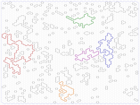
(a) n=1.4, x=0.6

(b) n=1.4, x=0.63

Figure 1: Samples of the loop $O(n)$ model for two nearby parameter values: the first in the predicted exponential decay regime and the second in the predicted macroscopic loops regime. The longest loops are colored for visibility.

Background. The loop $O(n)$ model contains other notable models of statistical mechanics models as special cases — e.g. the Ising model ($n=1$), critical percolation ($n=x=1$), the dimer model ($n=1,x=\infty$), self-avoiding walk ($n=0$), Lipschitz functions ($n=2$), proper 4-colorings ($n=2,x=\infty$), dilute Potts $(n=\sqrt{q},q$ integer), and the hard-hexagon model ($n\to\infty,nx^{6}\to\lambda$). Furthermore, the model serves as an approximate graphical representation of the spin $O(n)$ model, conjectured to be in the same universality class, which was the original motivation for its introduction [11]. See [34] for a recent survey on both $O(n)$ models.

A tantalizing 1982 prediction of Nienhuis [31], with later refinements [30, 6], [26, Section 5.6], [38, Section 2.2], is that the model exhibits macroscopic loops (i.e. loops surrounding balls of radius comparable to that of the domain) when

$$n\leq 2\quad\text{and}\quad x\geq x_{c}(n)=\frac{1}{\sqrt{2+\sqrt{2-n}}},$$ (1.1)

and has a conformal-invariant scaling limit $\mathrm{CLE}_{\kappa}$, where $\kappa=\kappa(n,x)$ may take all values in $[8/3,8]$. For all other parameter values, the length of the loop passing through a given vertex is expected to have exponential tails, uniformly in the domain and vertex.

Mathematical progress on the predictions is still quite limited. Conformal invariance has only been obtained in the classical cases of the critical Ising model ($n=1,x=\frac{1}{\sqrt{3}}$) [39, 10, 9] and critical site percolation on the triangular lattice ($n=x=1$) [37]. The rest of the progress is restricted to studying coarser properties of the loop structure, as summarized by Figure 2 and detailed below.

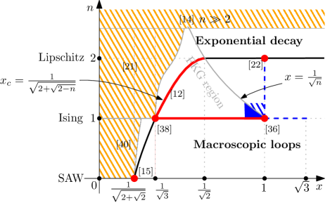
Figure 2: The predicted phase diagram for the loop $O(n)$ model. The critical line $x_{c}$ separating the regime of exponential decay from the regime of macroscopic loops is plotted in bold. The region $n\geq 1,x\leq\tfrac{1}{\sqrt{n}}$ where a dichotomy between the two behaviors is proved is denoted FKG region. Orange lines show regions where exponential decay is proved. Red dots or lines mark regions where macroscopic loops are proven to occur. The results of this paper are indicated in blue: macroscopic loops are established in the filled area, while exponential decay is ruled out in the dashed area and segments. Picture adapted from Glazman–Manolescu [21].

As mentioned above, loop lengths are predicted to follow one of two types of behaviors, according to the value of $n$ and $x$: either macroscopic loops appear, or the length of loops has exponential tail decay. However, other behaviors have not been ruled out in general. Recently, such a dichotomy has been established in the parameter range $n\geq 1,x\leq\tfrac{1}{\sqrt{n}}$ [12].

The only two cases where the loop $O(n)$ model was shown to exhibit a phase transition at $x=x_{c}(n)$ are $n=1$ (Ising model) and $n=0$ (self-avoiding walk). Exponential decay in the low-temperature Ising model ($x<1/\sqrt{3}$) [1] and existence of infinitely many loops around each vertex (in the unique Gibbs measure) for the critical and high-temperature Ising model ($1/\sqrt{3}\leq x\leq 1$) are classical. In the latter case, emergence of macroscopic loops follows from a general Russo–Seymour–Welsh (RSW) theory developed in [41] (or, alternatively, from the above dichotomy result). Recently, RSW theory was extended to a small interval in the antiferromagnetic regime ($1<x<1+\varepsilon$) [3]. The critical point of the self-avoiding walk on the hexagonal lattice was proven to equal $\tfrac{1}{\sqrt{2+\sqrt{2}}}$ in the celebrated work [15]. The walk was shown to scale to a straight line segment for smaller $x$ [25], and to be space-filling for larger $x$ [17].

The results known beyond the cases $n=0,1$ are as follows. Exponential decay was established when either $n>0,x<\tfrac{1}{\sqrt{2+\sqrt{2}}}+\varepsilon(n)$ [40] or $n>1,x<\tfrac{1}{\sqrt{3}}+\varepsilon(n)$ [21], by comparing to the behavior of the self-avoiding walk and Ising model, respectively. In addition, for sufficiently large $n$, exponential decay was proven for all $x>0$ (and an ordering transition was further established) [14]. Lastly, existence of macroscopic loops (as well as Russo–Seymour–Welsh type estimates) was recently shown to occur on the line $x=x_{c}(n)$ for $1\leq n\leq 2$ [12] and also at $n=2,x=1$ [22] (uniform Lipschitz functions).

Results. Existence of macroscopic loops has been established only in the rather sparse set of parameters discussed above. In fact, away from this set, even the seemingly modest goal of excluding exponential decay has not been achieved. The goal of the present work is to introduce a new technique for showing the existence of long loops in the loop $O(n)$ model. The technique applies in the vicinity of the critical percolation point $n=x=1$ and enables to derive the following three results:

• For some $\delta>0$, the model with $1\leq n\leq 1+\delta$ and $1-\delta\leq x\leq 1$ satisfies that, in any translation-invariant Gibbs measure, there is either an infinite path or infinitely many finite loops around the origin, almost surely. In the intersection of this regime and the proven dichotomy regime, i.e., when $1\leq n\leq 1+\delta$, $1-\delta\leq x\leq\tfrac{1}{\sqrt{n}}$, the result implies the existence of macroscopic loops in finite domains and the associated RSW theory.

  This is the first result to show that macroscopic loops occur on a regime of parameters with positive Lebesgue measure.

• For the antiferromagnetic Ising model in the regime of parameters $n=1,x\in(1,\sqrt{3}]$ it is shown that, in finite domains, there exists a loop whose diameter is comparable to that of the domain with uniformly positive probability. This implies that every Gibbs measure will have infinitely many loops surrounding the origin.

• In the parameter range $1\leq n\leq 2$, $x=1$, it is shown that the model on a torus exhibits a non-contractible loop with uniformly positive probability.

More precise statements as well as additional finite-volume consequences will appear in the three subsections below.

The new technique is based on a ‘XOR trick’. The XOR trick is straightforward in the case of critical percolation (see Section 1.4). Its application to other values of $n$ and $x$ is non-obvious; our analysis uses expansions in $n$ and $x$ and requires delicate control of the percolative properties of the resulting graphical representations. This control, in turn, relies on recent bounds on the site percolation threshold of planar graphs obtainable as Benjamini–Schramm limits.

Previous techniques for showing the existence of long loops relied on positive association (FKG) properties for a suitable spin representation; such representations are only known to exist in the regimes $n\geq 1,x\leq\tfrac{1}{\sqrt{n}}$ [12] and $n\geq 2,x\leq\tfrac{1}{\sqrt{n-1}}$ [22]. Among the merits of the new technique is that it applies in the absence of such FKG properties. A second merit is that the technique makes little use of the specific structure of the underlying hexagonal lattice and we expect it to apply more generally to the loop $O(n)$ model on a class of (possibly non-periodic) trivalent planar graphs.

Notation. In this paper, we embed the hexagonal lattice $\mathbb{H}$ and its dual triangular lattice $\mathbb{T}$ in the (complex) plane so that vertices of $\mathbb{T}$ (centers of faces of $\mathbb{H}$) are identified with numbers $k+\ell e^{i\pi/3}$ where $k,\ell\in\mathbb{Z}$. The face of $\mathbb{H}$ centered at the origin is denoted by $\mathsf{0}$.

For a positive integer $k$, and some face $f$ of $\mathbb{H}$, let $\Lambda_{k}(f)$ be the subgraph of $\mathbb{H}$ induced by all vertices bordering faces in the ball of radius $k$ around $f$ in $\mathbb{T}$. Below, in a slight abuse of notation, we refer to $\Lambda_{k}(f)$ as the ball of radius $k$ around $f$.

We say that a subgraph $\mathscr{D}$ of $\mathbb{H}$ is a domain if it consists of all vertices and edges surrounded by some self-avoiding cycle on $\mathbb{H}$ (including the cycle itself). In particular, balls defined above are examples of domains.

1.1 Results in the regime $1\leq n\leq 1+\delta$ and $1-\delta\leq x\leq 1$

It is convenient to first state our results in terms of infinite-volume measures and then pass to their finite-volume consequences. A measure $\mathbb{P}_{n,x}$ is an infinite-volume Gibbs measure of the loop $O(n)$ model, with edge-weight $x$, if $\mathbb{P}_{n,x}$ is supported on loop configurations (i.e. configurations of loops and bi-infinite paths) and satisfies the following property. Let $\omega$ be a sample from $\mathbb{P}_{n,x}$. Then, for any finite subgraph $\mathscr{D}$ of $\mathbb{H}$, conditioning on the restriction of $\omega$ to $\mathscr{D}^{c}$, almost surely, the distribution of $\omega$ is given by $\mathbb{P}_{\mathscr{D},n,x}^{\omega}$ (noting that this measure is determined by the restriction of $\omega$ to $\mathscr{D}^{c}$). The measure $\mathbb{P}_{n,x}$ is called translation-invariant if it is invariant under all translations preserving the lattice $\mathbb{H}$.

Theorem 1.

There exists $\delta>0$ such that the following holds. Let $\mathbb{P}_{n,x}$ be a translation-invariant Gibbs measure of the loop $O(n)$ model with

$$1\leq n\leq 1+\delta,\quad 1-\delta\leq x\leq 1.$$ (1.2)

Then,

$$\mathbb{P}_{n,x}\,\big{(}\{\text{$\exists$ bi-infinite path }\}\cup\{\text{every face is surrounded by infinitely many loops}\}\big{)}=1.$$

To place the theorem in context, we briefly discuss some of the beliefs regarding the number and structure of infinite-volume Gibbs measures. It is expected that the loop $O(n)$ model has a unique Gibbs measure for $0<n\leq 2$ and $0<x<\infty$ (for larger values of $n$, the model may exhibit multiple periodic Gibbs measures; see [18]). In addition, all Gibbs measures of the model with $n>0$ and $0<x<\infty$ are expected to be supported on loop configurations without bi-infinite paths. If these statements were established (for the regime (1.2)), the theorem would imply that the unique Gibbs measure has infinitely many loops surrounding every vertex, almost surely. However, both of these statements are currently only proven in the dichotomy regime $n\geq 1,x\leq\tfrac{1}{\sqrt{n}}$ under the assumption of translation-invariance [12].

The theorem rules out the possibility of exponential decay for the loops in the regime (1.2) (see Corollary 3 below). In the subregime where a dichotomy has been established, one thus concludes the existence of macroscopic loops in finite domains and the associated RSW theory. For instance, the following finite-volume statement is an immediate corollary of [12, Theorem 1].

Corollary 2.

There exist constants $\delta,c>0$ for which the following holds. Let $1\leq n\leq 1+\delta$ and $1-\delta\leq x\leq\tfrac{1}{\sqrt{n}}$. For any $k>1$ and any loop configuration $\xi$,

$$c\leq\mathbb{P}_{A_{k},n,x}^{\xi}[\exists\text{ a loop in $A_{k}$ surrounding }\mathsf{0}]\leq 1-c.$$ (1.3)

where $A_{k}:=\Lambda_{2k}(\mathsf{0})\setminus\Lambda_{k}(\mathsf{0})$ is an annulus with inner radius $k$ and outer radius $2k$.

We proceed to elaborate on the finite-volume consequences of Theorem 1 in the full regime (1.2). The first issue to address is to find a sequence of domains and boundary conditions for which the loop $O(n)$ model converges to a translation-invariant Gibbs measure in the thermodynamic (subsequential) limit. We use the natural choice of taking the domains to be graph balls of growing radius (more generally, Følner sequences) with the empty loop configuration as boundary conditions. To obtain translation-invariance in the limit, the configuration is considered from the point of view of a uniformly chosen vertex $v$. A technical point which must be addressed is that it is a priori unclear that thermodynamic limits are Gibbs measures (this may happen in models with long-range dependence, due to the possibility of multiple bi-infinite paths existing in the limit; see e.g. [24]). However, in our context of translation-invariant limit measures, the Gibbs property may be derived from a version of the Burton–Keane argument (see Proposition 27). Therefore, Theorem 1 implies that, as the domains grow, one either has a long loop (converging to the bi-infinite path) in the vicinity of $v$, or else one has longer and longer loops surrounding $v$. We may further conclude that the length of the loop passing through $v$ is not a uniformly integrable sequence of random variables (in particular, its moments of order larger than $1$ tend to infinity).

To give a precise statement, we begin with some definitions. For a face $f$ in $\mathscr{D}$, set $\mathscr{L}(f)$ to be the (random) length of the longest loop that borders $f$ in $\omega$ (setting it to zero if no such loop exists). We set $C_{r,R}(f)$ to be the event that there exists a loop in $\omega$ which intersects both $\Lambda_{r}(f)$ and $\Lambda_{R}(f)^{c}$; we also set $S_{r,R}(f)$ to be the event that there exists a loop in $\omega$ which is contained in $\Lambda_{R}(f)\setminus\Lambda_{r}(f)$ and surrounds $f$. A sequence of random variables $\{X_{k}\}$ is called uniformly integrable if

$$\lim_{r\to\infty}\limsup_{k\to\infty}\mathbb{E}[X_{k}\cdot 1_{X_{k}\geq r}]=0.$$

In particular, if the sequence $\{X_{k}\}$ is not uniformly integrable then $\lim_{k}\mathbb{E}|X_{k}|^{1+\epsilon}=\infty$ for all $\epsilon>0$.

Corollary 3.

There exists a constant $\delta>0$ for which the following holds. Assume that (1.2) holds. Let $\{\xi_{k}\}$ be loop configurations, $\omega_{k}$ be sampled from $\mathbb{P}_{\Lambda_{k}(\mathsf{0}),n,x}^{\xi_{k}}$, and $\mathbf{f}_{k}$ be a uniformly chosen face of $\Lambda_{k}(\mathsf{0})$, sampled independently. Then

$$\lim_{r\to\infty}\lim_{R\to\infty}\liminf_{k\to\infty}\mathbb{P}\left[C_{r,R}(\mathbf{f}_{k})\cup S_{r,R}(\mathbf{f}_{k})\right]=1.$$

Consequently, the sequence of random variables $\{\mathscr{L}(\mathbf{f}_{k})\}$ is not uniformly integrable.

1.2 Results for $n=1,x\in(1,\sqrt{3}]$ and antiferromagnetic Ising

In the next theorem, we show that, when $1<x\leq\sqrt{3}$, the loop $O(1)$ model exhibits at least one long loop. As we shall recall below, loops in loop $O(1)$ model are domain walls of an Ising model defined on the faces of $\mathbb{H}$. The correspondence is such that the Ising model is ferromagnetic when $x<1$, and is antiferromagnetic for $x>1$.

Theorem 4.

There exists a constant $c>0$ such that, for $n=1$ and any $1<x\leq\sqrt{3}$, any $k$ and any loop configuration $\xi$ on $\mathbb{H}$ that contains only finite loops,

$$\mathbb{P}_{\Lambda_{2k}(\mathsf{0}),1,x}^{\xi}(\mathsf{0}\text{ is surrounded by a loop of diameter greater than }k)\geq c.$$

Let $\tau$ be a spin configuration on vertices of $\mathbb{T}$ (or, equivalently, the faces of $\mathbb{H}$), that takes a value $+1$ or $-1$ at each vertex. Given a domain $\mathscr{D}$ in $\mathbb{H}$, the Ising model with parameter $\beta$ on the faces of $\mathscr{D}$ with boundary conditions $\tau$ is supported on spin configurations $\sigma$ that coincide with $\tau$ outside of $\mathscr{D}$ and is given by

$$\mathrm{Ising}_{\mathscr{D},\beta}^{\tau}(\sigma) =\frac{1}{Z_{\mathscr{D},\beta}^{\tau}}\cdot\exp\left(\beta\cdot\sum_{u\sim v}\sigma(u)\sigma(v)\right),$$ (1.4)

where $Z_{\mathscr{D},\beta}^{\tau}$ is a normalising constant and the sum runs over pairs of adjacent faces, at least one of which is in $\mathscr{D}$.

When positive, the parameter $\beta$ should be viewed as the inverse temperature for a ferromagnetic interaction model. In this case, the model is positively associated and satisfies Griffiths’ correlation inequalities that greatly aid the analysis; see eg. [20] for an introduction. On bipartite graphs, the models at $\beta$ and $-\beta$ are in bijection. Here, we focus on the antiferromagnetic case $\beta<0$ on the triangular lattice where much less is known. Theorem 4 implies the following corollary for the Ising model.

Corollary 5.

There exists a constant $c>0$ such that, for any $\beta\in[-\tfrac{1}{4}{\log 3},0]$, any $k>0$ and any boundary conditions $\tau$,

$$\mathrm{Ising}_{\Lambda_{2k}(\mathsf{0}),\beta}^{\tau}(\mathsf{0}\text{ is surrounded by a circuit of minuses of diameter}\geq k)\geq c.$$

Note that our approach does not produce Russo–Seymour–Welsh (RSW) statements for the antiferromagnetic Ising model. Specifically, we do not prove the surrounding cluster can be found in an annulus of a fixed aspect ratio. Such estimates are known [41] for $\beta\in[0,\tfrac{1}{4}{\log 3}]$; in a recent paper [3] the same was shown for $\beta\in(-\varepsilon,0)$ when $\varepsilon$ is small.

Our analysis also implies the following result on the Gibbs measures of the loop $O(1)$ and Ising models.

Corollary 6.

Let $\mathbb{P}_{1,x}$ be a Gibbs measure of the loop $O(1)$ model with $1<x\leq\sqrt{3}$. Then,

$$\mathbb{P}_{1,x}\,\big{(}\{\text{$\exists$ bi-infinite path }\}\cup\{\text{every face is surrounded by infinitely many loops}\}\big{)}=1.$$

Analogously, if $-\tfrac{1}{4}\log 3\leq\beta<0$, then any Gibbs measure $\mathrm{Ising}_{\beta}$ for the Ising model with parameter $\beta$ either includes a bi-infinite interface between pluses and minuses, or every face is surrounded by infinitely many finite interfaces.

1.3 Results for $n\in[1,2],x=1$ on a torus

In the next theorem, we show that, when $n\in[1,2],x=1$, the loop $O(n)$ model on a torus has a non-contractible loop with positive probability. Denote by $\mathsf{Tor}_{k,\ell}$ a $k\times\ell$ torus obtained by identifying faces on the opposite sides of a parallelogram domain on $\mathbb{H}$ that consists of faces $s+te^{i\pi/3}$, where $0\leq s\leq k$ and $0\leq t\leq\ell$ are integers. The measure $\mathbb{P}_{\mathsf{Tor}_{k,\ell},n,x}$ on loop configurations on $\mathsf{Tor}_{k,\ell}$ is defined in the same way as in the case of planar domains (no boundary conditions are necessary). We say that a loop is non-contractible if it has a non-trivial homotopy when considered as a subset of a continuous torus.

Theorem 7.

For any $n\in[1,2]$ and $x=1$ and any $k,\ell\in\mathbb{N}$,

$$\mathbb{P}_{\mathsf{Tor}_{k,\ell},n,1}(\text{there exists a non-contractible loop})\geq\tfrac{1}{4}.$$

Note that non-contractible loops are inherently “long” in the sense that their length is at least the side-length of the torus. It would be natural to extend this statement to planar domains; however, our proof relies on an additional symmetry of the torus.

1.4 Outline of the main tool: the XOR trick

The method that is at the heart of the proofs of this paper is the XOR trick. This trick makes use of the fact that loop configurations form a closed subgroup of $\{0,1\}^{E(\mathbb{H})}$ viewed as an abelian group under component-wise addition modulo $2$. Explicitly, we represent a loop configuration as a binary function on $E(\mathbb{H})$. For a loop configuration $\omega$ and a simple cycle $\Gamma$, define the configuration $\omega\,\oplus\,\Gamma$ as the symmetric difference of $\omega$ and $\Gamma$:

$$(\omega\,\oplus\,\Gamma)(e):=\omega(e)+1_{e\in\Gamma}\quad\text{ (mod 2)}\qquad\qquad\forall e\in E(\mathbb{H}).$$ (1.5)

Each vertex of $\mathbb{H}$ has an even degree in $\omega$ and $\Gamma$; therefore, the same is true for $\omega\,\oplus\,\Gamma$, meaning that the XOR operation is an involution on the set of loop configurations.

The next combinatorial lemma describes how the XOR operation produces large loops.

Lemma 8.

For any circuit $\Gamma$ that surrounds $\Lambda_{k}(\mathsf{0})$ and any loop configuration $\omega$, either $\omega$ or $\omega\,\oplus\,\Gamma$ contains a bi-infinite path or a loop of diameter at least $k$ that surrounds $\mathsf{0}$.

Proof.

Assume all loops in $\omega$ are finite. Let $\omega_{\Gamma}$ denote the union of loops in $\omega$ that intersect $\Gamma$. Since

$$(\omega_{\Gamma}\,\oplus\,\Gamma)\,\oplus\,\Gamma=\omega_{\Gamma},$$

all loops in $\omega_{\Gamma}\,\oplus\,\Gamma$ must intersect $\Gamma$. Note that

$$\omega\,\oplus\,\Gamma=\Gamma\,\oplus\,\omega_{\Gamma}\,\oplus\,(\omega\setminus\omega_{\Gamma})=(\Gamma\,\oplus\,\omega_{\Gamma})\cup(\omega\setminus\omega_{\Gamma}).$$

If no loop in $\omega$ surrounding $\mathsf{0}$ has diameter at least $k$, then no loop in $\omega_{\Gamma}$ surrounds $\mathsf{0}$. Then, since $\Gamma$ surrounds $\mathsf{0}$, the configuration $\Gamma\,\oplus\,\omega_{\Gamma}$ must contain a loop surrounding $\mathsf{0}$ that intersects $\Gamma$. The diameter of this loop must be at least $k$. ∎

In order to illustrate the use of Lemma 8, we provide a short ‘folkloric’ proof that, in the $O(1)$ loop model with $x=1$, the origin is surrounded by arbitrarily large loops with positive probability. As noted above, $\mathbb{P}_{\mathscr{D},1,1}$ coincides with the distribution of the boundary of site-percolation clusters when each face of $\mathbb{H}$ is open or closed with probability $1/2$, so this conclusion is not new and is in fact a significantly weaker version of the classical Russo–Seymour–Welsh (RSW) estimates [35, 36]. Nevertheless, the main point here is that the XOR trick is actually more robust than one might think and is applicable in settings where relatively little is understood about the underlying probability measure on loop configurations. A heuristic description of the argument can be seen in Figure 3.

Proposition 9.

For any $k$ and any loop configuration $\xi$ with no infinite paths, one has

$$\mathbb{P}_{\Lambda_{k}(\mathsf{0}),1,1}^{\xi}\,\big{(}\text{there exists a loop of diameter $\geq k$ surrounding $\mathsf{0}$}\big{)}\geq\tfrac{1}{2}.$$

Proof.

Let $A_{k}$ be the event that there exists a loop of diameter $\geq k$ surrounding $\mathsf{0}$. Set $\Gamma$ to be the boundary of $\Lambda_{k}(\mathsf{0})$. Since the  XOR-operation is measure-preserving, Lemma 8, together with the union bound, implies that

$$2\mathbb{P}_{\mathscr{D},1,1}^{\xi}(\omega\in A_{k})=\mathbb{P}_{\mathscr{D},1,1}^{\xi}(\omega\in A_{k})+\mathbb{P}_{\mathscr{D},1,1}^{\xi}(\omega\,\oplus\,\Gamma\in A_{k})\geq 1.$$ ∎

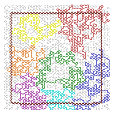
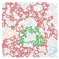
Figure 3: Left: an instance of the $\mathbb{P}_{\mathscr{D},1,1}$, with the longest loop in red. Middle: a large loop superimposed on the configuration. Right: the result of the XOR operation between the configuration and the loop. Again, the largest loop is in red. Note that parts of the orange and blue clusters are cut into smaller clusters by the operation.

Compared to this toy case $n=x=1$, the difficulty in the proofs of our main results lies in the fact that as soon as $n\neq 1$ or $x\neq 1$, the measure $\mathbb{P}_{\mathscr{D},n,x}^{\xi}$ is not uniform and hence the XOR operation is not measure-preserving. In order to surmount this difficulty, we consider an expansion around $n=x=1$ in both the $n$ and $x$ variables. Development in $n$ appears in Chayes–Machta [8], whereas expansion in $x$ corresponds to the classical Edwards–Sokal coupling [19] and its generalization by Newman [28, 29] to the antiferromagnetic case. This leads to a non-trivial measure assigned to defect sets of edges (in case of Theorem 4), loops (Theorem 7) or both (Theorem 1). Conditioned on these defect subgraphs, the remaining configuration is distributed according to the uniform measure on the complement and thus is invariant under XOR. Therefore, our goal is to show that these defect subgraphs allow for a large vacant circuit.

Acknowledgements

The authors would like to thank Michael Krivelevich for sharing knowledge about planar graphs, and Ioan Manolescu and Yinon Spinka for fruitful discussion of the work presented here and help with the figures.

AG, MH, and RP were supported in part by Israel Science Foundation grant 861/15 and the European Research Council starting grant 678520 (LocalOrder). NC was supported by Israel Science Foundation grant number 1692/17. AG was supported by the Swiss NSF grants P300P2_177848,  P3P3P2_177850, P2GEP_165093. MH was supported by the Zuckerman Postdoctoral Fellowship. RP and MH were further supported by Israel Science Foundation grant 1971/19.

2 $n=1,x\in(1,\sqrt{3}]$

The aim of this section is to prove Theorem 4. The proof is based on the well-known correspondence between the loop $O(1)$ model and the Ising model, with $x>1$ being mapped to the antiferromagnetic Ising model. The latter model can be represented as a conditioned FK-Ising model using Newman’s extension [28, 29] of the classical Edwards–Sokal coupling. Known results on the standard FK-Ising model will then imply that the XOR trick is applicable for the loop $O(1)$ model with $x\in(1,\sqrt{3})$, thus proving Theorem 4.

We fix $n=1$ until the end of this section.

2.1 Link to the Ising model

The loop $O(1)$ model on a domain $\mathscr{D}$ of $\mathbb{H}$ can be viewed as a domain wall, or low-temperature, representation of the Ising model on the faces of the lattice; see for example [20, Section 3.7.2]. The next lemma states this connection explicitly.

Recall that $\tau:\mathbb{T}\rightarrow\{-1,1\}$ is a spin configuration on the vertices of $\mathbb{T}$ — or, equivalently, the faces of $\mathbb{H}$. For a domain $\mathscr{D}$, we set $\mathscr{S}(\mathscr{D},\tau)$ to be the set of spin configurations that match $\tau$ on the faces of $\mathscr{D}^{c}$. Let $\mathrm{DW}(\tau)$ be the subgraph of $\mathbb{H}$ where $e\in\mathrm{DW}(\tau)$ if and only if the edge borders on two faces with different values of $\tau$.

Lemma 10.

Let $\tau$ be a spin configuration, and set $\xi=\mathrm{DW}(\tau)$. Then, for any domain $\mathscr{D}$, $\mathrm{DW}$ is a bijection from $\mathscr{S}(\mathscr{D},\tau)$ to $\mathscr{E}(\mathscr{D},\xi)$. Moreover, if $\sigma\in\mathscr{S}(\mathscr{D},\tau)$ and $\omega=\mathrm{DW}(\sigma)$, then

$$\mathbb{P}_{\mathscr{D},1,x}^{\xi}(\omega)=\mathrm{Ising}_{\mathscr{D},\beta}^{\tau}(\sigma),\text{ where }\beta=-\tfrac{1}{2}\log x.$$ (2.1)

Proof.

Since $\mathscr{D}^{c}$ is connected as a subset of $\mathbb{T}$, it is standard that $\mathrm{DW}$ is a bijection. Let us now study the push-back of the loop $O(1)$ measure under it. For any loop configuration $\omega$, its probability can be written in the following way:

$$\mathbb{P}_{\mathscr{D},1,x}^{\xi}(\omega) =\frac{1}{Z_{\mathscr{D},1,x}^{\xi}}\cdot x^{|\omega|}=\frac{1}{Z_{\mathscr{D},1,x}^{\xi}}\cdot x^{\#\{u\sim v\,:\,\sigma(u)\neq\sigma(v)\}}=\frac{1}{Z_{\mathscr{D},1,x}^{\xi}}\cdot\exp\Big{(}\log x\cdot\sum_{u\sim v}1_{\{\sigma(u)\neq\sigma(v)\}}\Big{)}$$

$$=\frac{1}{Z_{\mathscr{D},1,x}^{{}^{\prime}\,\tau}}\exp\Big{(}\beta\sum_{u\sim v}\sigma(u)\sigma(v)\Big{)}=\mathrm{Ising}_{\mathscr{D},\beta}^{\tau}(\sigma),$$

where $Z_{\mathscr{D},1,x}^{{}^{\prime}\,\tau}:=\tfrac{Z_{\mathscr{D},1,x}^{\xi}}{x^{|E(\mathscr{D})|/2}}$ and we used that $1_{\{\sigma(u)\neq\sigma(v)\}}=\tfrac{1}{2}-\tfrac{1}{2}\sigma(u)\sigma(v)$ and $\beta=-\tfrac{1}{2}\log x$. ∎

Observe that $x\in(0,1)$ implies $\beta>0$ and thus the law of $\sigma$ is that of a ferromagnetic Ising model on the faces of $\mathscr{D}$. The case $x=1$ corresponds to the uniform measure on all $\pm 1$ spin configurations on the faces of $\mathscr{D}$ – that is, to Bernoulli site-percolation of parameter $1/2$ on the faces of $\mathscr{D}$. Finally, $x>1$ implies $\beta<0$ and thus $\sigma$ has the law of an antiferromagnetic Ising model.

As was first shown by Onsager [32], the value $\beta=\frac{\log 3}{4}$, or equivalently $x=\frac{1}{\sqrt{3}}$, is the critical point for the ferromagnetic Ising model on the triangular lattice (see [2] for the explicit formula on the triangular lattice). Sharpness of the phase transition was established in [1] and implies that, when $\beta>\frac{\log 3}{4}$ (that is $x<\frac{1}{\sqrt{3}}$), the model is in an ordered phase, with exponentially small pockets of $-1$ in an environment of $+1$.

At the same time, when $0\leq\beta<\frac{\log 3}{4}$ (that is $\frac{1}{\sqrt{3}}<x\leq 1$), the model is in a disordered phase, with macroscopic clusters of both $+1$ and $-1$; this is a consequence of the proof in [41].

2.2 FK-Ising representation in the antiferromagnetic regime

In this section, our aim is to describe FK-type representations of the loop $O(1)$ model. For $0<x<1$, this is a classical Edwards–Sokal coupling [19] between the ferromagnetic Ising model and FK-Ising model (random-cluster model with $q=2$). For $x>1$ (antiferromagnetic Ising model), we will use the extension of this coupling suggested by Newman [28, 29]. In the case $x>1$, the resulting measure is a conditioned FK-Ising measure. The relation between this model and the standard FK-Ising model will be analyzed in Section 2.4.

Given a domain $\mathscr{D}$, define the dual domain $\mathscr{D}^{*}$ as a subgraph of the triangular lattice $\mathbb{T}$ induced on the set of vertices that correspond to faces bordering at least one edge of $\mathscr{D}$.

For the remains of this section, we will identify loop configurations on $\mathscr{D}$ with spin configurations on faces of $\mathscr{D}$ using the bijection of Lemma 10.

2.2.1 Ferromagnetic Ising model: $0<x<1$

For any $\sigma\in\mathscr{E}(\mathscr{D},\tau)$, we may write the Ising measure measure in the following way:

$$\mathrm{Ising}_{\mathscr{D},\beta}^{\tau}(\sigma)= \frac{1}{Z_{\mathscr{D},1,x}^{\xi}}\cdot x^{\#\{u\sim v\,:\,\sigma(u)\neq\sigma(v)\}}=\frac{x^{|E(\mathscr{D})|}}{Z_{\mathscr{D},1,x}^{\xi}}\cdot\left(\tfrac{1}{x}\right)^{\#\{u\sim v\,:\,\sigma(u)=\sigma(v)\}}$$

$$=\frac{x^{|E(\mathscr{D})|}}{Z_{\mathscr{D},1,x}^{\xi}}\cdot\prod_{u\sim v}(1+(\tfrac{1}{x}-1)1_{\sigma(u)=\sigma(v)})=\frac{x^{|E(\mathscr{D})|}}{Z_{\mathscr{D},1,x}^{\xi}}\cdot\sum_{\eta\subset E(\mathscr{D}^{*})}(\tfrac{1}{x}-1)^{|\eta|}\prod_{uv\in\eta}1_{\sigma(u)=\sigma(v)},$$

where $\xi=\mathrm{DW}(\tau)$, $\beta=-\tfrac{1}{2}\log x$.

The joint law of $\sigma$ and $\eta$ takes the form of the Edwards–Sokal coupling:

$$\mathrm{ES}_{\mathscr{D},x}^{\xi}(\sigma,\eta)=\frac{x^{|E(\mathscr{D})|}}{Z_{\mathscr{D},1,x}^{\xi}}\cdot(\tfrac{1}{x}-1)^{|\eta|}\prod_{uv\in\eta}1_{\sigma(u)=\sigma(v)}.$$ (2.2)

Viewing $\eta$ as a spanning subgraph of $\mathscr{D}^{*}$, the last term is the indicator that $\sigma$ has constant value on each connected component (cluster) of $\eta$. In the ferromagnetic case we will focus on the FK-Ising model with wired boundary conditions, that is $\xi=\emptyset$ or, alternatively, $\tau\equiv+1$. Then, all boundary clusters of $\eta$ in (2.2) are assigned $+1$ in $\sigma$ and, for all other clusters, the value of $\sigma$ can be chosen to be $+1$ or $-1$ independently.

The marginal distribution of $\mathrm{ES}_{\mathscr{D},x}^{1}$ on $\eta$ obtained after summing (2.2) over all spin configurations $\sigma$ takes the following form:

$$\varphi_{\mathscr{D},x}^{1}(\eta)=\frac{x^{|E(\mathscr{D})|}}{Z_{\mathscr{D},1,x}^{\emptyset}}\cdot(\tfrac{1}{x}-1)^{|\eta|}2^{k^{1}(\eta)},$$ (2.3)

where $|\eta|$ denotes the number of edges in $\eta$ and $k^{1}(\eta)$ is the number of clusters in $\eta$ when all boundary vertices of $\mathscr{D}^{*}$ are identified.

2.2.2 Antiferromagnetic Ising model: $x>1$

For this subsetion, we assume that $x>1$. Following the same steps as for the previous case, we find that:

$$\mathrm{Ising}_{\mathscr{D},\beta}^{\tau}(\sigma)= \frac{1}{Z_{\mathscr{D},1,x}^{\xi}}\cdot x^{\#\{u\sim v\,:\,\sigma(u)\neq\sigma(v)\}}=\frac{1}{Z_{\mathscr{D},1,x}^{\xi}}\cdot\prod_{u\sim v}(1+(x-1)1_{\sigma(u)\neq\sigma(v)})$$

$$= \frac{1}{Z_{\mathscr{D},1,x}^{\xi}}\cdot\sum_{\eta\subset E(\mathscr{D}^{*})}(x-1)^{|\eta|}\prod_{uv\in\eta}1_{\sigma(u)\neq\sigma(v)}.$$

The joint law of $\sigma$ and $\eta$ takes a form similar to (2.2):

$$\mathrm{ES}_{\mathscr{D},x}^{\xi}(\sigma,\eta)=\frac{1}{Z_{\mathscr{D},1,x}^{\xi}}\cdot(x-1)^{|\eta|}\prod_{uv\in\eta}1_{\sigma(u)\neq\sigma(v)}.$$ (2.4)

Viewing $\eta$ as a spanning subgraph of $\mathscr{D}^{*}$, the last term is the indicator that $\sigma$ defines a proper coloring of $\eta$ in $+1$ and $-1$, i.e. any two vertices linked by an edge of $\eta$ have different spins in $\sigma$. Letting $\mathrm{Bip}_{\xi}(\eta)$ denote the event that such a proper coloring exists, we observe that the event is nontrivial for every loop configuration $\xi$.

Repeating the same argument as above, we can see that the marginal distribution on $\eta$ for $x>1$ is given by

$$\varphi_{\mathscr{D},x}^{\xi}(\eta)=\frac{1}{Z_{\mathscr{D},1,x}^{\xi}}\cdot(x-1)^{|\eta|}2^{k^{0}(\eta)}\cdot 1_{\mathrm{Bip}_{\xi}(\eta)}.$$ (2.5)

In particular, we see that, for any $x>1$ and any loop configuration $\xi$, we have the relation

$$\varphi_{\mathscr{D},x}^{\xi}(\eta)=\varphi_{\mathscr{D},1/x}^{1}(\eta\,\mid\mathrm{Bip}_{\xi}(\eta)).$$ (2.6)

2.3 Input from the FK-Ising model

For $x<1$, $\varphi_{\mathscr{D},x}^{\mathrm{w}}$ is a standard wired FK-Ising measure. The classical result of Aizenman, Barsky, and Fernandez [1] proves that the FK-Ising model undergoes a sharp phase transition at the critical point (see [16] for a recent short proof). The exact value of the critical point on the triangular lattice is $x=\tfrac{1}{\sqrt{3}}$, as was first shown by Onsager [32] (see also [2] in which the triangular lattice is addressed explicitly). Together, these results imply that, for any $x\in(\tfrac{1}{\sqrt{3}},1)$, the model exhibits exponential decay – that is, there exists $c^{\prime}=c^{\prime}(x)>0$ such that, for any $k$,

$$\varphi_{\mathscr{D},x}^{1}(\mathsf{0}\text{ is connected to distance }k)<e^{-c^{\prime}k}.$$ (2.7)

The RSW theory developed in [13] for the FK-Ising model implies that, at the critical point $x=\tfrac{1}{\sqrt{3}}$, the connection probability decays polynomially in distance and probability to cross an annulus $\Lambda_{2k}(\mathsf{0})\setminus\Lambda_{k}(\mathsf{0})$ is bounded above and below uniformly in $k$.

We will only require the upper bounds, which hold for both $x\in(\tfrac{1}{\sqrt{3}},1)$ and $x=\tfrac{1}{\sqrt{3}}$.

Proposition 11.

Assume that $\Lambda_{2k}(\mathsf{0})\subset\mathscr{D}$ for some integer $k$. Then, for any $x\in[\tfrac{1}{\sqrt{3}},1)$, there exists a constant $c>0$ depending only on $x$ such that,

$$\varphi_{\mathscr{D},x}^{1}(\exists\text{ crossing from }\Lambda_{k}(\mathsf{0})\text{ to }\mathbb{T}\setminus\Lambda_{2k}(\mathsf{0}))<1-c.$$ (2.8)

We note that, for $x\in(\tfrac{1}{\sqrt{3}},1)$, the proposition follows from (2.7) and the union bound.

It is also known that, for any $0<x<1$, the FK-Ising measure $\varphi_{\mathscr{D},x}$ is positively associated (see eg. [23, Theorem 3.8]). Specifically, define a partial order on $\{0,1\}^{E(\mathscr{D}^{*})}$ by saying that $\eta\preceq\eta^{\prime}$ if $\eta(e)\leq\eta^{\prime}(e)$ for all $e\in E(\mathscr{D}^{*})$. We say that an event $A\subset\{0,1\}^{E(\mathscr{D}^{*})}$ is increasing if for any $\eta\in A$, $\eta\preceq\eta^{\prime}$ implies $\eta^{\prime}\in A$.

Lemma 12 (Positive association).

For any two increasing events $A,B\subset\{0,1\}^{E(\mathscr{D}^{*})}$ of positive probability, we have

$$\varphi_{\mathscr{D},x}^{1}(A\,|\,B)\geq\varphi_{\mathscr{D},x}^{1}(A).$$ (2.9)

Is is straightfoward to confirm that, for any loop configuration $\xi$, the event $\mathrm{Bip}_{\xi}(\eta)$ is decreasing in $\eta$. Combining this with (2.6), we conclude that, for any decreasing event $D$ and $x>1$,

$$\varphi_{\mathscr{D},x}^{\xi}(D)\leq\varphi_{\mathscr{D},1/x}^{1}(D).$$ (2.10)

2.4 Proof of Theorem 4, Corollary 5, and Corollary 6

Proof of Theorem 4.

Let $x\in(1,\sqrt{3}]$, and fix $k$ to be an integer. Consider the Edwards–Sokal measure on $\mathscr{D}=\Lambda_{2k}(\mathsf{0})$. For any circuit in $\mathscr{D}$ and a subgraph $\eta$ of $\mathscr{D}^{*}$, we say that the circuit crosses $\eta$ if one of its constituent edges is associated with an edge in $\eta$ (recalling that there is a bijection between the edges of $\mathscr{D}$ and $\mathscr{D}^{*}$). Define $\mathrm{Circ}_{k}$ to be the event that there exists a circuit $C$ on $\mathbb{H}$ entirely contained in the annulus $\Lambda_{2k}(\mathsf{0})\setminus\Lambda_{k}(\mathsf{0})$ which does not cross any edge of $\eta$. By planar duality, the event $\mathrm{Circ}_{k}$ is complementary to the existence of a crossing in $\eta$ from $\Lambda_{k}(\mathsf{0})$ to $\mathbb{T}\setminus\Lambda_{2k}(\mathsf{0})$. By observing that $\mathrm{Circ}_{k}$ is a decreasing event in $\eta$, we can use Proposition 11 and (2.10) to conclude that

$$\varphi_{\mathscr{D},x}^{\xi}(\mathrm{Circ}_{k})\geq\varphi_{\mathscr{D},1/x}^{1}(\mathrm{Circ}_{k})=1-\varphi_{\mathscr{D},1/x}^{1}(\exists\text{ crossing from }\Lambda_{k}(\mathsf{0})\text{ to }\mathbb{T}\setminus\Lambda_{2k}(\mathsf{0}))>c.$$ (2.11)

Assume $\eta\in\mathrm{Circ}_{k}$ and let $C\subset E(\mathbb{H})$ be the outermost circuit witnessing $\mathrm{Circ}_{k}$. Let $\sigma\in\mathscr{S}(\mathscr{D},\tau)$, and set $\omega=\mathrm{DW}(\sigma)$. We define $\sigma\,\oplus\,C$ to be the unique spin configuration in $\mathscr{S}(\mathscr{D},\tau)$ such that $\mathrm{DW}(\sigma\,\oplus\,C)=\omega\,\oplus\,C$; equivalently, $\sigma\,\oplus\,C$ is equal to $\sigma$ on the faces outside $C$, and equal to $-\sigma$ on the face on the interior. Thanks to (2.4) and the construction of $C$, we have that

$$\mathrm{ES}_{\mathscr{D},x}^{\xi}(\sigma,\eta)=\mathrm{ES}_{\mathscr{D},x}^{\xi}(\sigma\,\oplus\,C,\eta).$$

As in the proof of Proposition 9, either $\omega$ or $\omega\,\oplus\,C$ must contain a loop of diameter at least $k$ going around 0. Integrating over the probability of $\mathrm{Circ}_{k}$ and using Lemma 10, we find that

$$\mathbb{P}^{\xi}_{\Lambda_{2k}(\mathsf{0}),1,x}(\mathsf{0}\text{ is surrounded by a loop of diameter greater than }k)>\tfrac{1}{2}\cdot\varphi_{\mathscr{D},\tfrac{1}{x}}^{\xi}(\mathrm{Circ}_{k})>c/2,$$

completing the proof of the theorem.

∎

Proof of Corollary 5.

Let $\Gamma$ be the circuit of diameter greater than $k$ that surrounds $\mathsf{0}$. The sign of $\sigma$ must be constant along all faces that border $\Gamma$ on the interior, and constant on the faces that border $\Gamma$ on the exterior — and the two signs must be different. Thus, $\sigma$ will be identically $-1$ on exactly one of the two sets. Both sets form circuits surrounding $\mathsf{0}$, and the diameter of the smaller of the two is at least $k$. ∎

Proof of Corollary 6.

Fix $x\in(1,\sqrt{3}]$, and let $\mathbb{P}_{1,x}$ be a Gibbs measure for the loop $O(1)$ model. Since every Gibbs measure can be decomposed into an average over extremal Gibbs measures, it is sufficient to prove that every extermal Gibbs measure $\tilde{\mathbb{P}}_{1,x}$ satisfies

$$\tilde{\mathbb{P}}_{1,x}(\exists\text{ bi-infinite path})=1,\,\text{ or }\,$$

$$\tilde{\mathbb{P}}_{1,x}(\text{every face is surrounded by infinitely many loops})=1.$$

Since the existence of a bi-infinite path is a tail event, we may assume that there are no bi-infinite paths, $\tilde{\mathbb{P}}_{1,x}$-almost surely (otherwise, the probability is $1$ and we are done). Recall the events $C_{r,R}(\mathsf{0})$ and $S_{r,R}(\mathsf{0})$ defined in Section 1.1. Then, $S_{r}(\mathsf{0}):=\bigcup_{R>r}S_{r,R}(\mathsf{0})$ is the event that there exists a loop surrounding $\Lambda_{r}(\mathsf{0})$. By measurability and our assumption, we know that, for every positive integer $r$,

$$\lim_{R\to\infty}\tilde{\mathbb{P}}_{1,x}(C_{r,R}(\mathsf{0}))=0.$$

Set $R(r)$ to be the smallest integer such that $\tilde{\mathbb{P}}_{1,x}(C_{r,R}(\mathsf{0}))<c/2$, where $c$ is the constant from Theorem 4. If there exists a loop in $\Lambda_{2R(r)}(\mathsf{0})$ of diameter greater than $R$ that surrounds $\mathsf{0}$ and $C_{r,R}(\mathsf{0})$ does not occur, $S_{r}(\mathsf{0})$ must occur. Since $\tilde{\mathbb{P}}_{1,x}$ is a Gibbs measure for the loop $O(1)$ model, Theorem 4 implies that, for every $r$, $\tilde{\mathbb{P}}_{1,x}(S_{r}(\mathsf{0}))>c/2$. Furthermore,

$$\limsup_{r\to\infty}S_{r}(\mathsf{0})=\{\mathsf{0}\text{ is surrounded by infinitely many loops}\}.$$

In particular, the probability of the righthand event is at least $c/2$. Since this event is also a tail event, the extermaility of $\tilde{\mathbb{P}}_{1,x}$ implies that

$$\tilde{\mathbb{P}}_{1,x}(\mathsf{0}\text{ is surrounded by infinitely many loops})=1.$$

If one face is surrounded by infinitely many faces, so is every other face, and the proof is complete. ∎

3 $n\in(1,2],x=1$

In this section, we will prove Theorem 7 through an expansion of the loop $O(n)$ model in $n$, which was first used in [8]. A similar expansion was used in [22] and [21]. Once this expansion is established, a straightforward monotonicity argument, as well as simple geometric considerations on the torus, will yield the desired lower bound on the probability of finding a non-contractible loop.

Let $\omega_{r}$ and $\omega_{b}$ be two loop configurations on $\mathbb{T}_{k}^{2}$ (red and blue loops). The pair is coherent if the loops are disjoint. For any $n\geq 1$, define the measure $\rho_{\mathbb{T}_{k}^{2},n}$ by

$$\rho_{\mathbb{T}_{k}^{2},n}(\omega_{r},\omega_{b})=\frac{1}{Z_{\sf loop}(\mathbb{T}_{k}^{2})}\cdot(n-1)^{\ell(\omega_{b})}\cdot 1_{(\omega_{r},\omega_{b})\text{ is coherent}},$$ (3.1)

where $Z_{\sf loop}(\mathbb{T}_{k}^{2})$ is a normalizing constant. As is clear from the definition above, if one conditions on the $\omega_{b}$, the distribution of $\omega_{r}$ is the uniform measure on all configurations which are coherent with $\omega_{b}$. The next proposition shows that $\omega_{r}\cup\omega_{b}$ is distributed as a loop $O(n)$ model with edge weight $x=1$.

Proposition 13.

For any $n\geq 1$ the measure $\mathbb{P}_{\mathbb{T}_{k}^{2},n,1}$ is equal to the marginal of $\rho_{\mathbb{T}_{k}^{2},n}$ on $\omega_{r}\cup\omega_{b}$.

Proof.

Let $\omega$ be a loop configuration on $\mathbb{T}_{k}^{2}$, and let $\mathscr{C}(\omega)$ be the $2^{\ell(\omega)}$ distinct red/blue colorings of the loops of $\omega$. Each pair $(\omega_{r},\omega_{b})\in\mathscr{C}(\omega)$ is coherent, and therefore

$$\rho_{\mathbb{T}_{k}^{2},n}(\omega)=\frac{1}{Z_{\sf loop}(\mathbb{T}_{k}^{2})}\sum_{(\omega_{r},\omega_{b})\in\mathscr{C}(\omega)}(n-1)^{\ell(\omega_{b})}=\frac{1}{Z_{\sf loop}(\mathbb{T}_{k}^{2})}\cdot n^{\ell(\omega)},$$

where the final equality follows from a binomial-type expansion. ∎

The following lemma states the simple but essential observation that, whenever $n\in[1,2]$, $\omega_{r}$ stochastically dominates $\omega_{b}$.

Lemma 14.

For any increasing event $A$ and $n\in[1,2]$,

$$\rho_{\mathsf{Tor}_{k,\ell},n}[\omega_{r}\in A]\geq\rho_{\mathsf{Tor}_{k,\ell},n}[\omega_{b}\in A].$$

Proof.

If $\omega$ is distributed as $\mathbb{P}_{\mathsf{Tor}_{k,\ell},n,1}$, then the construction above implies that we can sample $(\omega_{r},\omega_{b})$ conditional on $\omega_{r}\cup\omega_{b}=\omega$ by coloring each loop blue with probability $(n-1)/n$, independently at random, and coloring the remaining loops red. Thus, conditional on $\omega$, $\omega_{r}$ and $\omega_{b}$ are distributed as a Bernoulli percolations on the loops of $\omega$. Whenever $n\in[1,2]$, $(n-1)/n\leq 1/2$, and thus the red percolation process dominates the blue percolation process. We conclude that, for any increasing event $A$,

$$\rho_{\mathsf{Tor}_{k,\ell},n}[\omega_{r}\in A] =\rho_{\mathsf{Tor}_{k,\ell},n}\left[\rho_{\mathsf{Tor}_{k,\ell},n}[\omega_{r}\in A\,\mid\,\omega_{r}\cup\omega_{b}=\omega]\right]$$

$$\geq\rho_{\mathsf{Tor}_{k,\ell},n}\left[\rho_{\mathsf{Tor}_{k,\ell},n}[\omega_{b}\in A\,\mid\,\omega_{r}\cup\omega_{b}=\omega]\right]$$

$$=\rho_{\mathsf{Tor}_{k,\ell},n}[\omega_{b}\in A]\qed.$$

It can be shown by induction that, for any loop configuration $\omega$ consisting only of contractible loops, there exists a spin configuration $\sigma$ assigning $\pm 1$ to the faces of $\mathsf{Tor}_{k,\ell}$, such that two adjacent faces have different spins if and only if their common edge belongs to $\omega$. We call such $\sigma$ a spin representation of $\omega$ (the term was introduced in [12]; for $n=1$, this is a classical low-temperature expansion for the Ising model [20, Sec. 3.7.2]). In the next lemma, we show that, for any configuration $\omega$ of contractible loops, applying the XOR operation with a non-contractible loop $\Gamma$ yields a non-contractible loop.

Lemma 15.

Let $\Gamma$ be a non-contractible loop. Then, for any loop configuration $\omega$ in $\mathsf{Tor}_{k,\ell}$, at least one of $\{\omega,\omega\,\oplus\,\Gamma\}$ includes a non-contractible loop.

Proof.

Assume $\omega$ and $\omega\,\oplus\,\Gamma$ contain only contractible loops. Let $\sigma_{\omega}$ and $\sigma_{\omega\,\oplus\,\Gamma}$ be their respective spin representations. Then, the product $\sigma_{\omega}\sigma_{\omega\,\oplus\,\Gamma}$ is a spin representation for $\Gamma$. However, such a representation cannot not exist, since removing a non-contractible loop keeps the torus connected (follows e.g. from the Euler’s formula). ∎

Let $\Gamma$ be a simple circuit in $\mathsf{Tor}_{k,\ell}$. Given $\omega_{b}$, we call $\Gamma$ blue-free if $\Gamma\cap\omega_{b}=\emptyset$. Similarly, $\Gamma$ is red-free if $\Gamma\cap\omega_{r}=\emptyset$. The duality lemma below shows that one can always find a non-contractible circuit that is blue- or red-free (see [22, Lemma 3.6] for a planar analogue).

Lemma 16.

Any loop configuration on a torus contains either a blue-free or a red-free non-contractible circuit.

Proof.

If the loop configuration contains a non-contractible loop, the statement is trivial. Assume all loops are contractible. Let $\sigma_{b}$ be a spin representation for $\omega_{b}$. Denote by $\eta_{b}$ the complement to $\omega_{b}$ in the set of all edges of $\mathsf{Tor}_{k,\ell}$. Let $\eta_{b}^{*}$ be a dual configuration, i.e. the set of pairs of adjacent faces of $\mathsf{Tor}_{k,\ell}$ having different spins in $\sigma_{b}$. By the standard duality (e.g. Euler’s formula), either $\eta_{b}$ or $\eta_{b}^{*}$ contains a non-contractible circuit. If this is $\eta_{b}$, then we are done, since such circuit is blue-free. Assume now that $\eta_{b}^{*}$ contains a non-contractible circuit $\tilde{\Gamma}$. By the definition of $\eta_{b}^{*}$, spins on along $\tilde{\Gamma}$ alternate. Applying the proof of [22, Lemma 3.6] to our setup mutatis mutandis we get that, by local modifications, $\tilde{\Gamma}$ can be made into a red-free non-contractible circuit. ∎

Proof of Theorem 7.

By Lemma 15, we may condition on $\omega_{b}$ and find that

$$\rho_{\mathsf{Tor}_{k,\ell},n}[\exists\text{ non-contractible loop}\,\mid\,\omega_{b}]\geq\tfrac{1}{2}\cdot 1_{\exists\text{ non-contractible blue-free circuit}}.$$

Taking expectations over $\omega_{b}$, we find that

$$\mathbb{P}_{\mathsf{Tor}_{k,\ell},n,1}[\exists\text{ non-contractible loop}]\geq\tfrac{1}{2}\cdot\rho_{\mathsf{Tor}_{k,\ell},1}[\exists\text{ non-contractible blue-free circuit}].$$ (3.2)

The existence of a blue-free circuit is a decreasing event in $\omega_{b}$; by taking complements and applying Lemma 14, the probability of the RHS of (3.2) is greater or equal than the same quantity for red-free circuits. By Lemma 16, the sum of the two probabilities is greater or equal to $1$. Together, this implies that the RHS of (3.2) is greater or equal than $1/4$. ∎

4 $n\in[1,1+\delta),x\in(1-\delta,1]$

This section will prove Theorem 1 and Corollaries 2 and 3. Here, we will expand the loop $O(n)$ model in both $n$ and $x$ simultaneously, which leads us to ‘defects’ that can be either loops or edges. Instead of working on subsets of $\mathbb{H}$ directly, we will generate auxiliary planar graphs from a infinite-volume loop configuration, which will converge to a (different) infinite planar graph, in the sense of Benjamini–Schramm convergence. Finally, we will show that the absence of defect-free circuits in the original domains can be coupled to the existence of infinite components in an appropriately chosen Bernoulli percolation process on the Benjamini–Scrhamm limits; the recent work [33] will be used to rule out this possibility at a small enough percolation parameter.

4.1 Defect-loop and -edge representation

For a finite domain $\mathscr{D}$ and a loop configuration $\xi$, let us consider the sample space $\bar{\mathscr{E}}(\mathscr{D},\xi)$ to be the set of all coherent triples $(\omega_{r},\omega_{b},\eta)$, where $\omega_{r}$ and $\omega_{b}$ are disjoint loop configurations satisfying $\omega_{r}\cup\omega_{b}\in\mathscr{E}(\mathscr{D},\xi)$, and $\eta\in\{0,1\}^{E(\mathscr{D})}$ satisfies $\eta\cap(\omega_{r}\cup\omega_{b})=\emptyset$. We refer to $\omega_{b}$ and $\eta$ as the defect loops and edges, respectively.

For any $0<x\leq 1$ and $n\geq 1$, define the measure $\mu_{\mathscr{D},n,x}^{\xi}$ by

$$\mu_{\mathscr{D},n,x}^{\xi}(\omega_{r},\omega_{b},\eta)=\frac{1}{Z_{\sf def}(\mathscr{D})}\cdot(n-1)^{\ell(\omega_{b})}\left(\tfrac{1}{x}-1\right)^{|\eta|}\cdot 1_{(\omega_{r},\omega_{b},\eta)\text{ is coherent}},$$ (4.1)

where $Z_{\sf def}(\mathscr{D})$ is a normalizing constant, and $|\eta|$ is the number of edges in $\eta$.

Proposition 17.

For any $n\geq 1$ and $x\in(0,1]$, the measure $\mathbb{P}_{\mathscr{D},n,x}^{\xi}$ is equal to the marginal of $\mu_{\mathscr{D},n,x}^{\xi}$ on $\omega_{r}\cup\omega_{b}$.

Proof.

Fix a pair of disjoint loop configurations $(\omega_{r},\omega_{b})$. By using a binomial-style expansion, it is easy to see that

$$\sum_{\eta\cap(\omega_{r}\cup\omega_{b})=\emptyset}\left(\tfrac{1}{x}-1\right)^{|\eta|}=\prod_{e\in E(\mathscr{D})\setminus(\omega_{r}\cup\omega_{b})}\left[1+\left(\tfrac{1}{x}-1\right)\right]=x^{-|E(\mathscr{D})\setminus(\omega_{r}\cup\omega_{b})|}.$$

Therefore, for any pair $(\omega_{r},\omega_{b})$ of disjoint loop configurations whose union is in $\mathscr{E}(\mathscr{D},\xi)$, the marginal of $\mu_{\mathscr{D},n,x}^{\xi}$ is

$$\mu_{\mathscr{D},n,x}^{\xi}(\omega_{r},\omega_{b})=\frac{x^{-|E(\mathscr{D})|}}{Z_{\sf def}(\mathscr{D})}\cdot(n-1)^{\ell(\omega_{b})}x^{|\omega(\sigma_{r})|+|\omega(\sigma_{b})|}.$$

To determine the marginal on $\omega_{r}\cup\omega_{b}$, we fix a loop configuration $\omega\in\mathscr{E}(\mathscr{D},\xi)$ and consider all possible colorings of its loops in red and blue. Summing over all such possibilities and using $n-1+1=n$, we get

$$\mu_{\mathscr{D},n,x}^{\xi}(\omega)=\frac{x^{-|E(\mathscr{D})|}}{Z_{\sf def}(\mathscr{D})}\cdot x^{|\omega|}\sum_{\omega_{b}\cup\omega_{r}=\omega}(n-1)^{\ell(\omega_{b})}=\frac{x^{-|E(\mathscr{D})|}}{Z_{\sf def}(\mathscr{D})}\cdot x^{|\omega|}n^{\ell(\omega)}=\mathbb{P}_{\mathscr{D},n,x}^{\xi}(\omega).\qed$$

Conversely, given $\omega\sim\mathbb{P}_{\mathscr{D},n,x}^{\xi}$ consider the random process producing $(\omega_{r},\omega_{b},\eta)$ constructed as follows:

• color each loop of $\omega$ that intersects with $\mathscr{D}$ blue with probability $\tfrac{n-1}{n}$, independently at random; the remaining loops will be red,

• let $\eta$ be an independent $(1-x)$-Bernoulli percolation on the edges in $\mathscr{D}\setminus\omega$.

If $\omega$ is sampled from an infinite-volume Gibbs measure $\mathbb{P}_{n,x}$, we can define $\mu_{n,x}$ by the above procedure, and observe that $\omega_{r}\cup\omega_{b}$ will also have the same law as $\mathbb{P}_{n,x}$.

Suppose $\Gamma$ is a simple circuit in $\mathscr{D}$. Given a triplet $(\omega_{r},\omega_{b},\eta)$, we call $\Gamma$ a defect-free if $\Gamma\cap(\omega_{b}\cup\eta)=\emptyset$. From (4.1), it is clear that the distribution of $\omega_{r}$ conditioned on $(\omega_{b},\eta)$ is uniform on all loop configurations that satisfy $\omega_{r}\cup\omega_{b}\in\mathscr{E}(\mathscr{D},\xi)$ and $\omega_{r}$ is disjoint from $\omega_{b}\cup\eta$. Both properties are preserved by the XOR operation with a defect-free circuit $\Gamma$, and thus,

$$\mu_{\mathscr{D},n,x}^{\xi}(\omega_{r},\omega_{b},\eta)=\mu_{\mathscr{D},n,x}^{\xi}(\omega_{r}\,\oplus\,\Gamma,\omega_{b},\eta).$$

Therefore, the XOR trick can be used to control the probability of large loops in terms of the probability existence of defect-free circuits.

The main proposition of this section concerns the existence of defect-free circuits in translation-invariant Gibbs measures of the loop $O(n)$ model not containing infinite paths when $n$ and $x$ are close enough to $1$.

Proposition 18.

There exists $\delta>0$ such that the following holds. Assume that

$$1\leq n\leq 1+\delta,\quad 1-\delta\leq x\leq 1.$$

Let $\mathbb{P}_{n,x}$ be a translation-invariant Gibbs measure for the loop $O(n)$ model with these parameters, and $\mu_{n,x}$ be its associated defect representation. If there are no bi-infinite paths $\mathbb{P}_{n,x}$-almost surely, then, for any positive integer $r$,

$$\mu_{n,x}(\exists\text{ a defect-free circuit surrounding }\Lambda_{r}(\mathsf{0}))=1.$$

Proof of Theorem 1, given Proposition 18.

We we may decompose the translation-invariant Gibbs measure $\mathbb{P}_{n,x}$ into a convex combination of ergodic measures. Therefore, it is sufficient to prove that any ergodic measure that has no bi-infinite paths (almost surely) must have infinitely many loops surrounding every face with probability $1$.

We may use Proposition 18, the lack of bi-infinite paths, and measurability to find an $R_{1}$ and $R_{2}$ such that

$$\mathbb{P}_{n,x}(\exists\text{ a loop crossing }\Lambda_{r}(\mathsf{0})\text{ and }\Lambda_{R_{1}}(\mathsf{0})^{c})<1/4$$

and

$$\mu_{n,x}(\exists\text{ a defect-free circuit in }\Lambda_{R_{2}}(\mathsf{0})\text{ surrounding }\Lambda_{R_{1}}(\mathsf{0}))>1/2.$$

Hence, with probability at least $1/4$, there exists a defect-free loop in $\Lambda_{R_{2}}(\mathsf{0})$ which surrounds $\Lambda_{R_{1}}(\mathsf{0})$ and is disjoint from every loop that intersects $\Lambda_{r}(\mathsf{0})$. By applying the XOR operation to $\Gamma$, the outermost loop witnessing the above event, we may conclude that

$$\mathbb{P}_{n,x}(\exists\text{ a loop surrounding }\Lambda_{r}(\mathsf{0}))>\tfrac{1}{8}.$$

The limsup of the above event as $r$ grows is equal to the existence of infinitely many loops surrounding $\mathsf{0}$; thus, this event must have probability of at least $1/8$. In fact, the probability must be $1$, since the measure was assumed to be ergodic and the event is translation invariant. We complete the proof by noting that, if $\mathsf{0}$ is surrounded by infinitely many loops, so is every other face. ∎

4.2 Percolation formulation of existence of defect-free circuits

Before proving Proposition 18, we wish to translate the existence of defect-free loops to the language of percolation processes. More specifically, given a domain $\mathscr{D}$, a loop configuration $\omega$ with no bi-infinite paths, and a face $f$ in $\mathscr{D}$, we will construct a planar graph $G_{\mathscr{D}}(\omega)$ and a 2-dependent site percolation process $\zeta$ so that we can bound the probability of finding a defect-free circuit in $\mathscr{D}$ that surrounds $\Lambda_{r}(f)$ from below using percolation probabilities involving $\zeta$. We then show that the process $\zeta$ is stochastically dominated by an independent site percolation of some intensity.

Fix a domain $\mathscr{D}$ and a loop configuration $\omega$ with no bi-infinite paths, and let $V_{\mathscr{D}}(\omega)$ be the set consisting of loops of $\omega$ that intersect $\mathscr{D}$, edges of $\mathscr{D}$ that are disjoint from $\omega$, and faces of $\mathscr{D}$. Define the projection map $\pi_{\omega}$ from the edges and faces of $\mathscr{D}$ to $V_{\mathscr{D}}(\omega)$ so that every edge belonging to a loop is sent to that loop; $\pi_{\omega}$ is the identity map on all other edges and faces. We define a graph $G_{\mathscr{D}}(\omega)$ whose vertex set is $V_{\mathscr{D}}(\omega)$, and where two vertices $u$ and $v$ of $G_{\mathscr{D}}(\omega)$ are linked by an edge if one of the following conditions is satisfied (see Figure 4):

1. $u=\pi_{\omega}(\mathrm{face}\,f)$, $v=\pi_{\omega}(\mathrm{edge}\,e)$, $e$ borders $f$;

2. $u=\pi_{\omega}(\mathrm{edge}\,e_{1})$, $v=\pi_{\omega}(\mathrm{edge}\,e_{2})$, $e_{1}$ and $e_{2}$ share an endpoint.

For a domain $\mathscr{D}$, we call the set of edges that border the external face its boundary. The image of this boundary under $\pi_{\omega}$ is called the boundary of $G_{\mathscr{D}}(\omega)$.

In the next lemma, we show that $G_{\mathscr{D}}(\omega)$ is a planar graph (morally, a triangulation) whose distances are at most doubled, compared to the triangular lattice $\mathbb{T}$. Set $\mathrm{dist}_{G_{\mathscr{D}}(\omega)}$ to be the graph distance in $G_{\mathscr{D}}(\omega)$, and define $B_{r}(v)$ to be the combinatorial ball of radius $r$ around a vertex $v$ in $G_{\mathscr{D}}(\omega)$ (with respect to this metric). Recall that, for any face $f$ in $\mathscr{D}$, $\Lambda_{r}(f)$ is the hexagonal lattice ball of radius $r$ induced by all vertices bordering faces of the ball of radius $r$ around $f$.

Lemma 19.

For any loop configuration $\omega$ without bi-infinite paths, there exists a planar graph on $V_{\mathscr{D}}(\omega)$ that coincides with $G_{\mathscr{D}}(\omega)$ once all multiple edges and self-loops are removed such that every face bordered by at least one non-boundary vertex of $G_{\mathscr{D}}(\omega)$ is a triangle. Additionally, for any face $f$ of $\mathscr{D}$, $B_{2r+1}(\pi_{\omega}(f))\supset\pi_{\omega}(\Lambda_{r}(f))$.

Proof.

Define $T_{\mathscr{D}}(\omega)$ to be the graph whose vertex set is the set of all faces of $\mathscr{D}$ and all edges contained in either $\mathscr{D}$ or a loop of $\omega$ that intersects $\mathscr{D}$. Two vertices of $T_{\mathscr{D}}(\omega)$ are neighbors in $T_{\mathscr{D}}(\omega)$ if they correspond to two edges that share an endpoint, or to a face and an edge that borders it.

We now consider the equivalence relation on the vertices of $T_{\mathscr{D}}(\omega)$ where $u$ is identified with $v$ if the two vertices correspond to edges of $\mathbb{H}$ that are on the same loop of $\omega$. The vertex set of the quotient graph is $V_{\mathscr{D}}(\omega)$. By construction, each equivalence class is a finite connected set, and therefore the quotient graph is planar. Since all faces of $T_{\mathscr{D}}(\omega)$ bordered by at least one non-boundary vertex of $G_{\mathscr{D}}(\omega)$ are triangles, the same holds for the quotient graph. Removing all multiple edges and self-loops gives $G_{\mathscr{D}}(\omega)$.

Next, consider a face $f$ of $\mathscr{D}$ and a face $g$ in $\Lambda_{r}(f)$. Then, the distance between $f$ and $g$ in $T_{\mathscr{D}}(\omega)$ is at most $2r$. This implies that the distance in $T_{\mathscr{D}}(\omega)$ between $f$ and any face or edge in $\Lambda_{r}(f)$ is at most $2r+1$. Since $G_{\mathscr{D}}(\omega)$ is obtained from $T_{\mathscr{D}}(\omega)$ by contraction and deletion of multiple edges and self-loops, the same inequality holds for distances in $G_{\mathscr{D}}(\omega)$. ∎

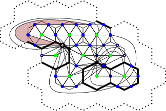
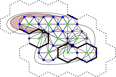
Figure 4: (left) A loop configuration $\omega$, with its intersection with a domain $\mathscr{D}$ in bold, and (right) $G_{\mathscr{D}}(\omega)$, with vertices associated to loops in black, edges disjoint from $\omega$ in blue, and face of $\mathscr{D}$ in green. Vertices with white circles in their center are boundary vertices.

To each vertex $\ell\in V_{\mathscr{D}}(\omega)$ corresponding to a loop in $\omega$, we will associate a subset of its neighbors in $G_{\mathscr{D}}(\omega)$, denoted by $I(\ell)$, and having the following properties:

1. vertices in $I(\ell)$ correspond to faces of $\mathscr{D}$,

2. $|I(\ell)|\leq 5$, and

3. for every pair of loops $\ell_{1},\ell_{2}$ such that $\mathrm{dist}_{G_{\mathscr{D}}(\omega)}(\ell_{1},\ell_{2})=2$, there exists $f\in I(\ell_{1})\cup I(\ell_{2})$ such that $f$ neighbors both $\ell_{1}$ and $\ell_{2}$.

Lemma 20.

There exists an association $I(\ell)$ which satisfies properties (P1), (P2), (P3).

Proof.

We use an auxiliary simple graph $G_{\mathsf{loop}}(\omega)$ on the loops of $\omega$, where two loops are linked by an edge if they border a common face $f$ of $\mathscr{D}$. We associate each edge of $G_{\mathsf{loop}}(\omega)$ with an (arbitrarily chosen) face of $\mathscr{D}$ that witnesses its existence. The graph $G_{\mathsf{loop}}(\omega)$ is simple and planar, and therefore, Euler’s formula implies that it must have at least one vertex of degree five or less. Let $\ell$ be the loop corresponding to this vertex, and set $I(\ell)$ to be the faces associated with the neighbors of $\ell$. We then remove $\ell$ and its neighboring edges, creating a new planar graph; iteration completes the proof. ∎

For the remainder of the paper, for any $\omega$, we will fix an association $I$ which satisfies the desired properties. Given $n\geq 1$ and $x\in(0,1]$, we define a percolation process $\zeta$ on the vertices of $G_{\mathscr{D}}(\omega)$ as follows:

• for any $\ell\in V_{\mathscr{D}}(\omega)$ corresponding to a loop of $\omega$, set $\zeta(\ell)=1$ with probability $(n-1)/n$, independently at random,

• for any $e\in V_{\mathscr{D}}(\omega)$ corresponding to an edge of $\mathscr{D}$, set $\zeta(e)=1$ with probability $1-x$, independently at random, and

• for any $f\in V_{\mathscr{D}}(\omega)$ corresponding to a face of $\mathscr{D}$, we set $\zeta(f)=1$ if $\zeta(e)=1$ for any edge $e$ of $\mathscr{D}$ bordering $f$. Additionally, if $f\in I(\ell)$ for some loop $\ell$, we set $\zeta(f)=1$ if $\zeta(\ell)=1$. Otherwise, set $\zeta(f)=0$.

The process $\zeta$ is a 2-dependent process, in the sense that $\{\zeta(s)\}_{s\in S}$ are independent random variables whenever $S$ is a subset of vertices of $V_{\mathscr{D}}(\omega)$ whose pairwise distances are all at least 3. We call a vertex $v\in G_{\mathscr{D}}(\omega)$ $\zeta$-open if $\zeta(v)=1$; a path is $\zeta$-open if all of its vertices are $\zeta$-open. We let $\nu_{G_{\mathscr{D}}(\omega),n,x}$ be the measure on $\{0,1\}^{V_{\mathscr{D}}(\omega)}$ associated with $\zeta$. For any $A,B$ subsets of the vertices of $G_{\mathscr{D}}(\omega)$, let $\{A\leftrightarrow B\}\subset\{0,1\}^{V_{\mathscr{D}}(\omega)}$ denote the event that there is a $\zeta$-open path from some vertex of $A$ to some vertex of $B$. Let $\partial G_{\mathscr{D}}(\omega)$ denote the set of boundary vertices of $G_{\mathscr{D}}(\omega)$.

Proposition 21.

Let $\omega$ be a loop configuration and $\mathscr{D}$ be a domain. Then, for any $n\geq 1$, $x\in(0,1]$, face $f$ in $\mathscr{D}$, $r\in\mathbb{N}$,

$$\begin{split}\mu_{\mathscr{D},n,x}^{\omega}[\exists\text{ a defect-free circuit surrounding }&\Lambda_{r}(f)\mid\omega_{r}\cup\omega_{b}=\omega]\\ &\geq\nu_{G_{\mathscr{D}}(\omega),n,x}[B_{2r+2}(\pi_{\omega}(f))\not\leftrightarrow\partial G_{\mathscr{D}}(\omega)].\end{split}$$

Proof.

By Lemma 19, we can add multiple edges and self-loops to $G_{\mathscr{D}}(\omega)$ in such a way that the resulting graph $G^{\Delta}_{\mathscr{D}}(\omega)$ is still planar and all faces bordered by at least one non-boundary vertex of $G_{\mathscr{D}}(\omega)$ are triangles. This operation does not alter percolation probabilities for any site percolation process. By the standard duality for site percolation on a triangulation, either the $\zeta$-open cluster of $B_{2r+2}(\pi_{\omega}(f))$ reaches the boundary of $G_{\mathscr{D}}(\omega)$ or the outer boundary of this cluster forms a $\zeta$-closed circuit:

$$\begin{split}\nu_{G_{\mathscr{D}}(\omega),n,x}&[B_{2r+2}(\pi_{\omega}(f))\not\leftrightarrow\partial G_{\mathscr{D}}(\omega)\mid\omega_{r}\cup\omega_{b}=\omega]\\ &=\nu_{G_{\mathscr{D}}(\omega),n,x}[\exists\text{ a }\zeta\text{-closed circuit surrounding }B_{2r+2}(\pi_{\omega}(f))].\end{split}$$

Now, we claim that, if there exists a $\zeta$-closed circuit surrounding $B_{2r+2}(\pi_{\omega}(f))$, there also exists a $\zeta$-closed circuit which surrounds $B_{2r+1}(\pi_{\omega}(f))$ and consists only of vertices that correspond to loops of $\omega$ and edges of $\mathscr{D}$. To prove this claim, we consider a simple circuit $\mathscr{C}=\{v_{0},\dots,v_{N}=v_{0}\}$ of $\zeta$-closed vertices. We assume that this circuit is minimal, in the sense that, whenever $v_{i},v_{j}$ are adjacent in $G_{\mathscr{D}}(\omega)$, $|i-j|=1$.

The claim follows if we can show that, whenever $\mathscr{C}$ includes some vertex $v_{i}$ that corresponds to a face of $\mathscr{D}$, we can locally modify $\mathscr{C}$ in order to bypass $v_{i}$. Let $N(v_{i})$ be the set of neighbors of $v_{i}$ in $G_{\mathscr{D}}(\omega)$. By minimality, $v_{i-1}$ and $v_{i+1}$ are not neighbors, and $\mathscr{C}$ does not contain any other element of $N(v_{i})$. Therefore, we can partition $N(v_{i})\setminus\{v_{i-1},v_{i+1}\}$ into two non-trivial components — one in the interior of $\mathscr{C}$, and the other in the exterior of $\mathscr{C}$. If one of these components contains only $\zeta$-closed vertices, we may bypass $v_{i}$, possibly increasing or decreasing the distance to $\pi_{\omega}(f)$ by one.

Otherwise, there exist two $\zeta$-open vertices $u_{1},u_{2}\in N(v_{i})$ that are separated from one another by $\mathscr{C}$. By the definition of $\zeta$ on faces of $\mathscr{D}$, this implies that $u_{1}$ and $u_{2}$ must correspond to loops of $\omega$. By (P3), there must be a face in $I(u_{1})\cup I(u_{2})$ neighboring both $u_{1}$ and $u_{2}$. By definition of $\zeta$, this face is $\zeta$-open. But it must also be a member of $\mathscr{C}$, which is $\zeta$-closed. This is a contradiction, and the claim follows.

Now, given a loop $\ell$ in $\omega$, we color $\ell$ blue if $\zeta(\ell)=1$ (and red otherwise). Given an edge $e$ that corresponds to a vertex of $G_{\mathscr{D}}(\omega)$, set it to be a defect edge if $\zeta(e)=1$. This constructs a coupling between $\zeta$, distributed as $\nu_{G_{\mathscr{D}}(\omega),n,x}$, and the triple $(\omega_{r},\omega_{b},\eta)\in\bar{\mathscr{E}}(\mathscr{D},\omega)$, distributed as $\mu_{\mathscr{D},n,x}^{\omega}(\cdot\mid\omega_{r}\cup\omega_{b}=\omega)$. In particular, $\zeta$-closed vertices of $G_{\mathscr{D}}(\omega)$ correspond either to red loops of $\omega$, to non-defect edges of $\mathscr{D}$, or to faces of $\mathscr{D}$.

Finally, assume there exists a ($\zeta$-closed) circuit $\mathscr{C}$ which surrounds $B_{2r+1}(\pi_{\omega}(f))$ and contains only vertices corresponding to red loops and non-defect edges. By Lemma 19, $\mathscr{C}$ also surrounds $\pi_{\omega}(\Lambda_{r}(f))$. By connectivity of $G_{\mathscr{D}}(\omega)$, the union of the (red) loops and (non-defect) edges corresponding to vertices in $\mathscr{C}$ contains a (defect-free) circuit surrounding $\Lambda_{r}(f)$; by inclusion of events, the proposition follows. ∎

The proof can be used to derive the following corollary.

Corollary 22.

In the setup of Proposition 21, if $\mathrm{dist}_{G_{\mathscr{D}}(\omega)}(\pi_{\omega}(f),\partial G_{\mathscr{D}}(\omega))>R\geq 2r+2$, then

$$\begin{split}\mu_{\mathscr{D},n,x}^{\omega}[\exists\text{ a defect-free circuit in }&B_{R}(\pi_{\omega}(f))\text{ surrounding }\Lambda_{r}(f)\mid\omega_{r}\cup\omega_{b}=\omega]\geq\\ &\nu_{G_{\mathscr{D}}(\omega),n,x}[B_{2r+2}(\pi_{\omega}(f))\not\leftrightarrow B_{R}(\pi_{\omega}(f))^{c}].\end{split}$$ (4.2)

The final proposition of this section proves that $\zeta$ can be dominated by a truly independent percolation process. Let $\mathrm{Ber}_{p}$ denote an independent $p$-Bernoulli percolation on the vertices of $G_{\mathscr{D}}(\omega)$ — i.e. $\mathrm{Ber}_{p}(v)=1$ with probability $p$ and $\mathrm{Ber}_{p}(v)=0$ with probability $1-p$ for every vertex of $G_{\mathscr{D}}(\omega)$, independently at random. We also use the notation $\preceq_{\mathsf{st}}$ to indicate stochastic domination of measures

Proposition 23.

Let $\omega$ be a loop configuration on $\mathscr{D}$ and let $\nu_{G_{\mathscr{D}}(\omega),n,x}$ be the percolation process on the graph $G_{\mathscr{D}}(\omega)$ defined above. There exists a continuous function $\mathbf{p}(n,x):[1,\infty)\times(0,1]$ with $\mathbf{p}(1,1)=0$ such that $\nu_{G_{\mathscr{D}}(\omega),n,x}\preceq_{\mathsf{st}}\mathrm{Ber}_{\mathbf{p}(n,x)}$.

Proof.

For every edge $e$ of $\mathscr{D}$, let us define a random variable $X_{e}$ that assigns to every vertex of $G_{\mathscr{D}}(\omega)$ zero or one according to the following law. Let $f,f^{\prime}$ be two faces of $\mathscr{D}$ bordered by $e$ (if $e$ is a boundary edge of $\mathscr{D}$, there is only one such face). Then, $X_{e}(f)=X_{e}(f^{\prime})=X_{e}(e)=1$ with probability $1-x$, $X_{e}(f)=X_{e}(f^{\prime})=X_{e}(e)=0$ with probability $x$; $X_{e}(v)=0$ always for any other vertex of $G_{\mathscr{D}}(\omega)$.

Set $p_{x}:=(1-x)^{1/3}$. By a standard coupling argument, we can realize $(X_{e})_{e\in E(\mathscr{D})}\in\{0,1\}^{V_{\mathscr{D}}(\omega)}$ in such a way that

$$X_{e}\preceq_{\mathsf{st}}\sum_{v=e,f,f^{\prime}}\mathrm{Ber}_{p_{x}}(v).$$ (4.3)

Explicitly, we can couple the left- and right-hand random variables above by setting $X_{e}(f)=X_{e}(f^{\prime})=X_{e}(e)=1$ if and only if all three Bernoulli random variables on the right-hand side are $1$, and $X_{e}\equiv 0$ otherwise. Under this coupling, the left-hand side is pointwise smaller than the right-hand side.

Next, and independent of the previous construction, let us define, for every loop $\ell$ of $\omega$, a random variable $Y_{\ell}$: $Y_{\ell}(v)=1$ for every $v\in I(\ell)\cup\{\ell\}$ with probability $\tfrac{n-1}{n}$, $Y_{\ell}(v)=1$ for every $v\in I(\ell)\cup\{\ell\}$ with probability $\tfrac{1}{n}$; $Y_{\ell}(v)=0$ always for any other vertex of $G_{\mathscr{D}}(\omega)$. Set $p_{n}:=\left(\tfrac{n-1}{n}\right)^{1/6}$. As above and since $|I(\ell)|\leq 5$ by Property (P2), we can realize $(Y_{\ell})_{e\in E(\mathscr{D})}$ on $\{0,1\}^{V_{\mathscr{D}}(\omega)}$ in such a way that

$$Y_{\ell}\preceq_{\mathsf{st}}\sum_{v\in I(\ell)\cup\{\ell\}}\mathrm{Ber}_{p_{n}}(v).$$ (4.4)

Finally let us define the process $Z$ as the pointwise maximum of the pair of independent processes $X$ and $Y$. By construction, $Z$ is distributed according to $\nu_{G_{\mathscr{D}}(\omega),n,x}$. From (4.3) and (4.4), $Z$ is dominated by a non-homogeneous independent Bernoulli percolation process on vertices of $G_{\mathscr{D}}(\omega)$, where the parameter at every edge is $p_{x}$, at every loop is $p_{n}$, and at every face $f$ is $p_{x}$ times the number of edges that border $f$ plus $p_{n}$ times the number of loops $\ell$ with $f\in I(\ell)$. The latter quantity can be trivially bounded above by $6p_{x}+3p_{n}$ and the proposition follows with

$$\mathbf{p}(n,x)=6p_{x}+3p_{n}=6(1-x)^{1/3}+3\left(\tfrac{n-1}{n}\right)^{1/6}.\qed$$

4.3 Benjamini–Schramm limits

The event on the right side of (4.2) is a local event, for the percolation $\zeta$, in the sense that it depends only on the value of $\zeta$ restricted to vertices that are in $B_{R+1}(\pi_{\omega}f)$. Such events can be studied in an infinite limit by using the framework of Benjamini–Schramm convergence [5], which we now recall. For a finite graph $G$, let $U_{G}$ be the uniform distribution on the vertices of $G$. Given a sequence of, possibly random, finite graphs $\{G_{k}\}$, we say that $\{G_{k}\}$ converges in the Benjamini–Schramm sense to the random rooted graph $(G,o)$, whose distribution is denoted $\mathbb{P}_{G}$, if, for every fixed $r$ and finite graph $H$,

$$U_{G_{k}}[B_{r}(o_{k})=H]\to\mathbb{P}_{G}[B_{r}(o)=H].$$

We wish to take subsequential limits of the sequence of random graphs $G_{\Lambda_{k}(\mathsf{0})}(\omega)$, where $\omega$ is some loop configuration; however, existence of such limits is not immediate. In [5], the graphs considered were assumed to have uniformly bounded degrees, making compactness trivial. Unfortunately, not every sequence of graphs has a Benjamini–Schramm limit — for example, if $G_{k}$ is a star on $k$ vertices, $B_{2}(v)=G_{k}$ for every vertex in $G_{k}$, and thus $U_{G_{k}}[B_{2}(o_{k})=H]$ converges to zero for every finite $H$. Therefore, some condition on the graph sequence is needed to maintain compactness in the general setting. In our case, a uniform integrability condition on the degrees of the graph is sufficient for existence of sub-sequential limits.

Precisely, we say that a sequence of random graphs $\{G_{k}\}$ has uniformly integrable degrees if

$$\lim_{r\to\infty}\limsup_{k\to\infty}\mathbb{E}_{k}\left[\frac{\sum_{v}\deg_{G_{k}}(v)1_{\deg_{G_{k}}(v)\geq r}}{|V(G_{k})|}\right]=0,$$

where $\deg_{G_{k}}(v)$ stands for the degree of $v$ in $G_{k}$, $V(G_{k})$ is the set of vertices of $G_{k}$, and $\mathbb{E}_{k}$ is the expectation operator for the random graph sequence.

Proposition 24.

If $\{G_{k}\}$ has uniformly integrable degrees, then there exists a subsequence that converges in the Benjamini-Schramm sense.

We note that a very similar statement, which was phrased for a deterministic sequence of graphs $\{G_{k}\}$, was shown in [4, Theorem 3.1].

Proof.

Let us denote by $\overline{\mathbb{P}}_{k}$ the joint distribution of both the random graph $G_{k}$ and a uniformly chosen vertex $o_{k}$ on that graph. For any finite, rooted graph $H$ and any integer $r$, $\{\overline{\mathbb{P}}_{k}[B_{r}(o_{k})=H]\}$ is a sequence of real numbers between zero and one, and hence we can extract a subsequence on which this quantity converges. Since there are countably many finite, rooted graphs and integers $r$, a diagonalization argument can be used to find a subsequence on which $\overline{\mathbb{P}}_{k}[B_{r}(o_{k})=H]$ converges for all $H$ and $r$. This defines a sequence of limit measures $\overline{\mathbb{P}}[B_{r}(o)=\cdot]$ for every integer $r$.

In order to prove that $\{G_{k}\}$ converges in the sense of Benjamini-Schramm, we must show that all the resulting measures are probability measures — i.e. that no probability mass escapes to infinity. To prove this tightness condition, it is sufficient to prove that, for every integer $r$ and $\varepsilon>0$, there exists $T=T(r,\varepsilon)$ such that

$$\overline{\mathbb{P}}[|B_{r}(o)|>T^{r}]\leq\varepsilon.$$

For any pair of integers $k$ and $T_{0}$, define the (random) sets

$$S_{0}(T_{0}):=\{v\in G_{k}:\deg_{G_{k}}(v)>T_{0}\},S_{i}(T_{0}):=\{u:u\sim S_{i-1}(T_{0})\}\setminus S_{i-1}(T_{0}),$$

and set $p_{i}(T_{0}):=\overline{\mathbb{P}}_{k}[o_{k}\in S_{i}(T_{0})]$ (we suppress the dependence of these parameters on $k$ for notational convenience; all estimates below will hold uniformly in $k$). For any vertex $v\not\in\cup_{i=0}^{r-1}S_{i}(T_{0})$, the ball of radius $r$ can contain at most $T_{0}^{r}$ vertices. Hence it will be sufficient to prove that, for any $\varepsilon>0$, there exists a $T_{0}$ sufficiently large so that $\sum_{i=0}^{r-1}p_{i}(T_{0})<\varepsilon$.

Let $(T_{0},\dots,T_{r-2})$ be a decreasing sequence of integers (to be determined later), and define $\delta_{i}$ by

$$\delta_{i}=\overline{\mathbb{E}}_{k}[\deg_{G_{k}}(o_{k})1_{\deg_{G_{k}}(o_{k})\geq T_{i}}].$$ (4.5)

By the uniform integrability assumption, $\delta_{i}$ can be made arbitrarily small by increasing $T_{i}$. We also partition $S_{i}(T_{0})$ into two sets: $S_{i}^{+}$ is the set of vertices in $S_{i}(T_{0})$ of degree greater than $T_{i}$, and $S_{i}^{-}$ are those of degree at most $T_{i}$.

Since the choice of $o_{k}$ is uniform once we condition on $G_{k}$,

$$p_{i}(T_{0})=\mathbb{E}_{k}\left[\frac{|S_{i}(T_{0})|}{|G_{k}|}\right] \leq\mathbb{E}_{k}\left[\frac{\sum_{v\in S_{i-1}}\deg_{G_{k}}(v)}{|G_{k}|}\right]$$

$$\leq\mathbb{E}_{k}\left[\frac{T_{i-1}\cdot|S_{i-1}^{-}|+\sum_{v\in S^{+}_{i-1}}\deg_{G_{k}}(v)}{|G_{k}|}\right]$$

$$\leq T_{i-1}\cdot p_{i-1}(T_{0})+\delta_{i-1},$$ (4.6)

where the final inequality follows by bounding $|S_{i-1}^{-}|$ by $|S_{i-1}|$ and noting that the second sum divided by the volume is bounded above by the expectation in (4.5). We set $M_{r-1}:=1$ and $M_{i}=M_{i+1}T_{i}+1$, and note by induction that, for any $0\leq j\leq r-1$

$$\sum_{i=j}^{r-1}p_{i}(T_{0})\leq M_{j}\cdot p_{j}(T_{0})+\sum_{i=j+1}^{r-1}M_{i}\delta_{i-1}.$$ (4.7)

Indeed, for $j=r-1$ the inequality is trivial; then one substitutes $p_{r-1}(T_{0})$ on the RHS using (4.6) and obtains the inequality for $j=r-2$; the proof continues in the same way by induction. In particular, (4.7) implies that

$$\sum_{i=0}^{r-1}p_{i}(T_{0})\leq M_{0}\cdot p_{0}(T_{0})+\sum_{i=1}^{r-1}M_{i}\cdot\delta_{i-1}.$$ (4.8)

It remains to bound the RHS. Since $M_{i}$ is independent of $(T_{0},T_{1},\dots T_{i-1})$, we may choose the $T_{i}$’s, starting from $T_{r-2}$, so that $M_{i}\cdot\delta_{i-1}<\varepsilon/2^{i+1}$. By Markov’s inequality,

$$T_{0}\cdot p_{0}(T_{0})=T_{0}\cdot\overline{\mathbb{P}}_{k}[\deg_{G_{k}}(o_{k})>T_{0}]\leq\overline{\mathbb{E}}_{k}\left[\deg_{G_{k}}(o_{k})1_{\deg_{G_{k}}(o_{k})>T_{0}}\right],$$

and therefore $\lim_{T_{0}\to\infty}T_{0}\cdot p_{0}(T_{0})=0$, uniformly in $k$. Since $M_{0}$ is a linear function of $T_{0}$ (whose coefficients depend on $(T_{1},\dots,T_{r-2})$), we can increase $T_{0}$ to ensure that $M_{0}\cdot p_{0}(T_{0})<\varepsilon/2$. Substituting this in (4.8) completes the proof. ∎

The notion of boundary also plays an important role in our analysis. A sequence of graphs $\{G_{k}\}$ with boundary is called Følner if

$$\lim_{k\to\infty}\tfrac{|\partial G_{k}|}{|G_{k}|}=0.$$

A corollary of the earlier lemma involves the typical distance from the root to the boundary of a Følner sequence of graphs.

Corollary 25.

Let $\{G_{k}\}$ be a Følner sequence of graphs with uniformly integrable degrees. Then, for any $r\in\mathbb{N}$,

$$\lim_{k\to\infty}U_{G_{k}}[\mathrm{dist}_{G_{k}}(o_{k},\partial G_{k})\leq r]=0.$$

Proof.

Assume, for the sake of contradiction, that there exist $K,\varepsilon>0$ such that, for infinitely many $k>K$,

$$U_{G_{k}}[\mathrm{dist}_{G_{k}}(o_{k},\partial G_{k})\leq r]>\varepsilon.$$

This implies that, for infinitely many $k>K$,

$$\left|\bigcup_{u\in\partial G_{k}}B_{r}(u)\right|>\varepsilon|V(G_{k})|.$$

Now, consider the auxiliary graph sequence $\{\tilde{G}_{k}\}$, given by adding one vertex to $G_{k}$ and connecting it to every vertex in $\partial G_{k}$. No subsequene of this sequence can converge in the Benjamini–Schramm sense, as, with probability at least $\varepsilon$, a ball of radius $2r+2$ around $o_{k}$ has volume at least $\varepsilon|V(G_{k})|$, which grows to infinity with $k$. However, since $\{G_{k}\}$ has uniformly integrable degrees and is a Følner sequence, the sequence $\{\tilde{G}_{k}\}$ must also have uniformly integrable degrees. This contradicts Lemma 24, as required. ∎

The final ingredient is a statement about Bernoulli site on Benjamini–Schramm limits of finite planar graphs.

Theorem 26.

[33] There exists a $p_{0}>0$ such that following holds. Let $\{G_{k}\}$ be a sequence of, possibly random, finite simple planar graphs that converges to a limit $(G,o)$ in the sense of Benjamini–Schramm. Then

$$\mathrm{Ber}_{p_{0}}\left(\exists\text{ an infinite }\text{open path in }G\right)=0,$$

where $\mathrm{Ber}_{p}$ is the independent $p$-Bernoulli percolation on vertices of $G$.

We emphasize that the choice of $p_{0}$ is independent of the sequence of graphs $\{G_{k}\}$.

4.4 Proof of Proposition 18

Proof.

Let $\mathbb{P}_{n,x}$ be a translation-invariant Gibbs measure for the loop $O(n)$ model, where the parameters satisfy (1.2), and $\mu_{n,x}$ be its associated defect representation. By assumption, if $\omega$ is sampled from $\mathbb{P}_{n,x}$, then it contains contains no bi-infinite paths, almost surely. For an integer $r$, a face $f$, and a domain $\Lambda_{k}(\mathsf{0})$ including $f$, let $\mathrm{Circ}_{r,k}(f)$ be the event that there exists a defect-free circuit in $\Lambda_{k}(\mathsf{0})$ which surrounds $\Lambda_{r}(f)$. We also let $\mathbf{f}_{k}$ be a uniformly chosen face in $\Lambda_{k}(\mathsf{0})$. By translation invariance of $\mu_{n,x}$, the probability of surrounding $\Lambda_{r}(\mathsf{0})$ by a defect-free circuit is the same as surrounding $\Lambda_{r}(\mathbf{f}_{k})$ by a defect-free circuit. By inclusion of events and the Gibbs property, we have that, for any integer $k$,

$$\mu_{n,x}\left[\exists\text{ a defect-free circuit surrounding }\Lambda_{r}(\mathsf{0})\right] \geq\mu_{n,x}\left[\mathrm{Circ}_{r,k}(\mathbf{f}_{k})\right]$$

$$\geq\mathbb{P}_{n,x}\left[\mu^{\omega}_{\Lambda_{k}(\mathsf{0}),n,x}[\mathrm{Circ}_{r,k}(\mathbf{f}_{k})\mid\omega_{r}\cup\omega_{b}=\omega]\right].$$

Since the left-hand side does not depend on $k$, we may take the liminf as $k$ goes to infinity; by Fatou’s lemma, we find that it is sufficient to prove that, for $\mathbb{P}$-almost every $\omega$,

$$\lim_{k\to\infty}\mu^{\omega}_{\Lambda_{k}(\mathsf{0}),n,x}[\mathrm{Circ}_{r,k}(\mathbf{f}_{k})\mid\omega_{r}\cup\omega_{b}=\omega]=1.$$

We set $\mathrm{Ber}_{p,G_{\Lambda_{k}(\mathsf{0})}(\omega)}$ to be independent $p$-Bernoulli percolation on $G_{\Lambda_{k}(\mathsf{0})}(\omega)$. We pick $\delta$ sufficiently small so that $\mathbf{p}(n,x)\leq p_{0}$ for any $(n,x)$ satisfying (1.2), where $\mathbf{p}(n,x)$ is the function in Proposition 23 and $p_{0}$ is defined in Theorem 26. Combining Propositions 21 and 23, it is sufficient to prove that

$$\lim_{R\to\infty}\limsup_{k\to\infty}\,\mathrm{Ber}_{p_{0},G_{\Lambda_{k}(\mathsf{0})}(\omega)}\left[B_{2r+2}\left(\pi_{\omega}\left(\mathbf{f}_{k}\right)\right)\leftrightarrow\partial G_{\Lambda_{k}(\mathsf{0})}(\omega)\right]=0.$$

Let $o_{k}$ be a uniformly chosen vertex in $V_{\Lambda_{k}(\mathsf{0})}(\omega)$. Let $F_{\Lambda_{k}(\mathsf{0})}\subset V_{\Lambda_{k}(\mathsf{0})}(\omega)$ be the set of vertices associated with faces of $\Lambda_{k}(\mathsf{0})$. The distribution of $o_{k}$ conditioned on the event $\{o_{k}\in F_{\Lambda_{k}(\mathsf{0})}\}$ is identical $\pi_{\omega}(\mathbf{f}_{k})$. The construction of $G_{\Lambda_{k}(\mathsf{0})}(\omega)$ ensures that

$$|V_{\Lambda_{k}(\mathsf{0})}(\omega)|\leq 7|F_{\Lambda_{k}(\mathsf{0})}|,$$

and therefore $U_{G_{\Lambda_{k}}(\mathsf{0})}(o_{k}\in F_{\Lambda_{k}(\mathsf{0})})\geq 1/7$; in particular, $\pi_{\omega}(\mathbf{f}_{k})$ is uniformly absolutely continuous with respect to $o_{k}$. By Corollary 22, we are done as soon as we show that

$$\begin{split}\lim_{R\to\infty}\limsup_{k\to\infty}\,\mathrm{Ber}_{p_{0},G_{\Lambda_{k}(\mathsf{0})}(\omega)}\left[B_{2r+2}\left(o_{k}\right)\leftrightarrow B_{R}^{c}\left(o_{k}\right)\right]&=0\quad\text{and}\\ \lim_{k\to\infty}\,\,U_{G_{\Lambda_{k}(\mathsf{0})}(\omega)}\left[\mathrm{dist}(o_{k},\partial G_{\Lambda_{k}(\mathsf{0})}(\omega))\leq R\right]&=0\end{split}$$ (4.9)

Suppose that $\{G_{\Lambda_{k}(\mathsf{0})}(\omega)\}$ has uniformly integrable degrees. By Proposition 24, there exists an infinite planar rooted graph $(G(\omega),o)$ that is a (subsequential) Benjamini–Schramm limit of the above sequence of graphs. Since the event $B_{2r+2}\left(o_{k}\right)\leftrightarrow B_{R}^{c}$ is local, in the sense that it is measurable with respect to the restriction of the Bernoulli percolation to a ball of radius $R+1$ around $o_{k}$, we find that

$$\lim_{k\to\infty}\,\mathrm{Ber}_{p_{0},G_{\Lambda_{k}(\mathsf{0})}(\omega)}\left[B_{2r+2}\left(o_{k}\right)\leftrightarrow B_{R}^{c}\left(o_{k}\right)\right]=\mathrm{Ber}_{p_{0},G(\omega)}\left[B_{2r+2}\left(o\right)\leftrightarrow B_{R}^{c}\left(o\right)\right],$$

where the limit may be taken along a converging subsequence. Since the events are decreasing in $R$, the limit of the probability is equal to the probability of the infinite intersection — namely, the probability that $B_{2r+2}(o)$ intersects an infinite open path. By Theorem 26 and our choice of $p_{0}$, no such path exists, and hence the double limit in (4.9) is zero, as desired. Under the assumption of uniformly integrable degrees, the second stipulation of (4.9) follows from Corollary 25 (since $\{\Lambda_{k}(\mathsf{0})\}$ is Følner, so is $\{G_{\Lambda_{k}(\mathsf{0})}(\omega)\}$).

To complete the proof, we must show that $\{G_{\Lambda_{k}(\mathsf{0})}(\omega)\}$ has uniformly integrable degrees. The degree of any vertex in $G_{\Lambda_{k}(\mathsf{0})}(\omega)$ corresponding to a loop $\ell$ in $\omega$ is bounded above by $4|\ell\cap\Lambda_{k}(\mathsf{0})|$, as the degree is bounded by the number of faces and edges in $\Lambda_{k}(\mathsf{0})$ that share a vertex with $\ell$; and the degrees of other vertices $G_{\Lambda_{k}(\mathsf{0})}(\omega)$ are at most $6$. Thus, for any $r>6$,

$$\sum_{v}\deg(v)\,1_{\deg(v)\geq r}\leq 4\,\sum_{\ell}|\ell\cap\Lambda_{k}(\mathsf{0})|\cdot 1_{|\ell\cap\Lambda_{k}(\mathsf{0})|\geq r/4},$$ (4.10)

where the right-hand sum is over the loops $\ell$ in $\omega$ that intersect $\Lambda_{k}(\mathsf{0})$. Every loop that has $m$ edges in $\Lambda_{k}(\mathsf{0})$ must border at least $m/6$ faces of $\Lambda_{k}(\mathsf{0})$, and every face borders at most three distinct loops. Therefore,

$$4\,\sum_{\ell}|\ell\cap\Lambda_{k}(\mathsf{0})|\cdot 1_{|\ell\cap\Lambda_{k}(\mathsf{0})|\geq r/4} \leq 20\,\sum_{\ell,f\in F_{\Lambda_{k}(\mathsf{0})}}1_{|\ell\cap\Lambda_{k}(\mathsf{0})|\geq r/4,f\text{ borders }\ell}$$

$$\leq 60\,\sum_{f\in F_{\Lambda_{k}(\mathsf{0})}}1_{f\text{ borders a loop of length }\geq r/4}.$$

Since $|V_{\Lambda_{k}(\mathsf{0})}(\omega)|>|F_{\Lambda_{k}(\mathsf{0})}|$, the inequality (4.10) implies that, for every $\omega$ and $k$,

$$\tfrac{1}{|V_{\Lambda_{k}(\mathsf{0})}(\omega)|}\sum_{v}\deg(v)1_{\deg(v)\geq r}\leq 60\cdot U_{F(\Lambda_{k}(\mathsf{0}))}\left(\mathbf{f}_{k}\text{ borders a loop of length }\geq r/4\right),$$

where $U_{F(\Lambda_{k}(\mathsf{0}))}$ is a uniform measure on the faces of $\Lambda_{k}(\mathsf{0})$. Taking expectation over $\omega$, we find that the sequence of graphs is uniformly integrable if

$$\lim_{r\to\infty}\limsup_{k\to\infty}\,\,\mathbb{P}_{n,x}\left(\mathbf{f}_{k}\text{ borders a loop of length }\geq r/4\right)=0.$$

By translation invariance of $\mathbb{P}_{n,x}$, we may replace $\mathbf{f}_{k}$ with $\mathsf{0}$. This operation makes the probability independent of $k$, and thus the double limit reduces to the probability that $\mathsf{0}$ borders an infinite path. By our assumption, all loops of $\omega$ are finite $\mathbb{P}_{n,x}$-a.s. ∎

4.5 Proofs of Corollaries 2 and 3

Before we prove the remaining corollaries, we must address a technical point: we have not shown that there exists any translation-invariant Gibbs measure for the loop $O(n)$ model. Such constructions usually follow by taking thermodynamic limit points of finite volume measures. However, in models with long-range interaction such as the loop O(n) model, it is theoretically possible for thermodynamic limit points to fail to have the Gibbs property. For example, [24] shows that this occurs for the random-cluster measure on $d$-regular trees whenever $d\geq 3$ and $q>2$. Fortunately, this pathology can be ruled out in our setup, in which we examine the loop $O(n)$ model around a typical face. The proof relies on the uniqueness results of Burton and Keane [7].

We let $\{\xi_{k}\}$ be a sequence of loop configurations, and recall that $\mathbf{f}_{k}$ is a uniformly chosen face in $\Lambda_{k}(\mathsf{0})$. Let $\tau_{f}$ be the unique translation map of $\mathbb{H}$ which maps $\mathsf{0}$ to $f$. Define $\tilde{\mathbb{P}}^{\,\xi_{k}}_{k,n,x}:=\mathbb{P}^{\,\xi_{k}}_{\Lambda_{k}(\mathsf{0}),n,x}\left(\tau^{-1}_{\mathbf{f}_{k}}\cdot\right)$, where $\mathbf{f}_{k}$ is chosen independently of the loop configuration. In words, $\tilde{\mathbb{P}}^{\,\xi_{k}}_{k,n,x}$ samples a loop configuration from $\mathbb{P}_{\Lambda_{k}(\mathsf{0}),n,x}^{\,\xi_{k}}$, and then recenters the configuration around a uniformly chosen face.

Proposition 27.

For any $(n,x)\in(0,\infty)^{2}$ and any sequence of loop configuration $\{\xi_{k}\}$, any subsequential limit of $\{\tilde{\mathbb{P}}^{\,\xi_{k}}_{k,n,x}\}$ is a translation-invariant Gibbs measure with at most one bi-infinite path.

We note that, unlike all other statements in this paper, this proposition holds regardless of the value of $n$ and $x$. A similar statement appears in [23, Theorem 4.31], in the context of the random cluster model, and in [27, Section 6.3], as a corollary of a more general framework. We include a proof for completeness.

Proof.

Consider a sequence of measures $\{\tilde{\mathbb{P}}^{\xi_{k}}_{k,n,x}\}$ which converges to an infinite-volume measure $\mathbb{P}_{n,x}$. We claim that $\mathbb{P}_{n,x}$ is translation-invariant. It is enough to show this invariance for the translation by one to the right, which we denote by $\tau_{1}$. Let $A$ be an arbitrary event supported on a finite ball, and consider the difference $\tilde{\mathbb{P}}^{\xi_{k}}_{k,n,x}(A)-\tilde{\mathbb{P}}^{\xi_{k}}_{k,n,x}(\tau_{1}A)$. By definition,

$$\tilde{\mathbb{P}}^{\xi_{k}}_{k,n,x}(A)-\tilde{\mathbb{P}}^{\xi_{k}}_{k,n,x}(\tau_{1}A) =\mathbb{P}^{\xi_{k}}_{\Lambda_{k}(\mathsf{0}),n,x}(\tau_{\mathbf{f}_{k}}A)-\mathbb{P}^{\xi_{k}}_{\Lambda_{k}(\mathsf{0}),n,x}(\tau_{\mathbf{f}_{k}}\tau_{1}A)$$

$$=\tfrac{1}{|F(\Lambda_{k}(\mathsf{0}))|}\cdot\mathbb{E}^{\xi_{k}}_{\Lambda_{k}(\mathsf{0}),n,x}\left[\sum_{f\in F(\mathscr{D}_{k})}1_{\tau_{f}A}-\sum_{f^{\prime}\in F(\tau_{1}\Lambda_{k}(\mathsf{0}))}1_{\tau_{f^{\prime}}A}\right]$$

$$\leq\tfrac{2|\partial\Lambda_{k}(\mathsf{0})|}{|F(\Lambda_{k}(\mathsf{0}))|}\stackrel{{\scriptstyle[}}{{k}}\to\infty]{}{\longrightarrow}0,$$

where the inequality follows from the fact that all faces except those on the boundary are counted in both sums.

Now, let $\omega$ be distributed as $\mathbb{P}_{n,x}$, and define $\sigma$ to be a configuration on $\{-1,1\}^{\mathbb{T}}$ given by assigning $\pm 1$ to $\mathsf{0}$, uniformly at random, and then letting

$$\sigma_{f}=\sigma_{\mathsf{0}}\cdot(-1)^{\#\text{edges of }\omega\text{ on a path from }\mathsf{0}\text{ to }f}.$$

Informally, we choose $\sigma$ at $\mathsf{0}$ uniformly at random, and then switch the value of $\sigma$ every time we cross an edge of $\omega$. Since $\omega$ is a loop configuration, $\sigma$ is well defined and is independent of the path chosen in the definition above. In Section 2.1, we used this construction to associate the loop $O(1)$ model with the Ising model; for more general values of $n$, the distribution of $\sigma$ will be non-local and more complicated.

By definition, the pushforward measure on $\sigma$ is translation-invariant. Furthermore, the measure has the uniform-finite energy property, in the sense that the probability $\sigma_{f}=+1$ is uniformly bounded away from zero and one even if one conditions on the state of all other spins. Indeed, switching the sign of $\sigma_{f}$ is equivalent to mapping $\omega$ to $\omega\,\oplus\,\Gamma_{f}$, where $\Gamma_{f}$ is the loop of length six surrounding $f$. This operation changes the number of loops by at most three, and the number of edges by at most six, whence

$$\mathbb{P}^{\xi_{k}}_{\Lambda_{k}(\mathsf{0}),n,x}(\omega\,\oplus\,\Gamma_{f})\geq c(n,x)\cdot\mathbb{P}^{\xi_{k}}_{\Lambda_{k}(\mathsf{0}),n,x}(\omega),\text{ where }c(n,x)=\min\{n^{3},n^{-3}\}\cdot\min\{x^{6},x^{-6}\}.$$

Using the standard Burton-Keane argument [7, Theorem 2], this implies that there is at most one infinite cluster of $+1$’s in $\sigma$, $\mathbb{P}_{n,x}$-almost surely; by symmetry, the same holds for $-1$’s. The correspondence between $\sigma$ and $\omega$ implies that a bi-infinite path in $\omega$ will occur as an interface between an infinite cluster of $+1$’s and an infinite cluster of $-1$’s. Since there is at most one of each, there can only be one such interface.

To complete the proof, we are left to prove that $\mathbb{P}_{n,x}$ is a Gibbs measure for the loop $O(n)$ model with edge weight $x$ — that is, to confirm that the marginal of $\mathbb{P}_{n,x}$ to any finite subgraph $\mathscr{D}$, conditioned on the restriction of $\omega$ to $\mathscr{D}^{c}$, is $\mathbb{P}_{\mathscr{D},n,x}^{\omega}$. Fix $\mathscr{D}$ to be a finite subgraph containing $\mathsf{0}$, and let $R$ be an integer such that $\Lambda_{R}(\mathsf{0})$ contains $\mathscr{D}$. We set $\mathscr{T}_{R}$ to be the event that $\omega$ contains at most two disjoint paths that intersect both $\mathscr{D}$ and $\Lambda_{R}(\mathsf{0})^{c}$. Since $\mathbb{P}_{n,x}$ is supported on configurations with at most one bi-infinite path, we have that

$$\lim_{R\to\infty}\mathbb{P}_{n,x}[\mathscr{T}_{R}]=1.$$ (4.11)

Let $\omega$ be a loop configuration distributed as $\mathbb{P}_{n,x}$, and fix some other loop configuration $\omega_{0}$. Then, using Levy’s Upwards Theorem and (4.11), and the definition of $\mathbb{P}_{n,x}$, we find

$$\mathbb{P}_{n,x}(\omega=\omega_{0}\text{ on }\mathscr{D}\,|\,\omega\text{ on }\mathscr{D}^{c}) =\lim_{R\rightarrow\infty}\mathbb{P}_{n,x}(\omega=\omega_{0}\text{ on }\mathscr{D}\,|\,\omega\text{ on }\Lambda_{R}(\mathsf{0})\setminus\mathscr{D})$$

$$=\lim_{R\rightarrow\infty}\mathbb{P}_{n,x}(\omega=\omega_{0}\text{ on }\mathscr{D}\,|\,\omega\text{ on }\Lambda_{R}(\mathsf{0})\setminus\mathscr{D},\,\mathscr{T}_{R})$$

$$=\lim_{R\rightarrow\infty}\lim_{k\to\infty}\,\tilde{\mathbb{P}}^{\xi_{k}}_{k,n,x}(\omega=\omega_{0}\text{ on }\mathscr{D}\,|\,\omega\text{ on }\Lambda_{R}(\mathsf{0})\setminus\mathscr{D},\mathscr{T}_{R}).$$

Let $\mathscr{T}^{(i)}_{R}$ be the event that $\omega$ contains precisely $i$ crossings from $\mathscr{D}$ to $\Lambda_{R}(\mathsf{0})^{c}$. Since the loop $O(n)$ model is supported on loop configurations, $\mathscr{T}^{(i)}_{R}=\emptyset$ when $i$ is odd. Thus, $\mathscr{T}_{R}=\mathscr{T}^{(0)}_{R}\cup\mathscr{T}^{(2)}_{R}$. If $\mathscr{T}^{(0)}_{R}$ occurs, then every loop that intersects $\mathscr{D}$ is contained in $\Lambda_{R}(\mathsf{0})$; in particular, the measure in $\mathscr{D}$ is determined by the restriction of $\omega$ to $\Lambda_{R}(\mathsf{0})$.

As above, we denote by $\mathbf{f_{k}}$ a face in $\Lambda_{k}(\mathsf{0})$ chosen uniformly. By definition of the loop $O(n)$ measure on finite domains, we deduce that, for any $k$,

$$\tilde{\mathbb{P}}^{\xi_{k}}_{k,n,x}(\omega=\omega_{0}\text{ on }\mathscr{D}\,|\,\omega\text{ on }\Lambda_{R}(\mathsf{0})\setminus\mathscr{D},\mathscr{T}^{(0)}_{R},\mathrm{dist}(\mathbf{f_{k}},B_{k}^{c})>R)=\frac{x^{|\omega_{0}|}n^{\ell(\omega_{0})}}{Z^{\omega}_{\mathscr{D},n,x}}=\mathbb{P}^{\omega}_{\mathscr{D},n,x}(\omega_{0}),$$ (4.12)

where $|\omega_{0}|$ is the number of edges in $\omega_{0}\cap\mathscr{D}$, and $\ell(\omega_{0})$ is the number of loops intersecting $\mathscr{D}$ (as there are no bi-infinite paths intersecting $\mathscr{D}$ under our assumptions). Note that the condition on $\mathbf{f_{k}}$ insures that none of the edges in $\mathscr{D}$ belong to $\Lambda_{k}(\mathbf{f_{k}})^{c}$ — that is, none of these edges are fixed by the boundary conditions $\xi_{k}$.

The relation (4.12) is precisely the desired Gibbs condition, modulo the restriction on $\mathbf{f_{k}}$. Luckily, for any fixed $R$, the probability that $\mathrm{dist}(\mathbf{f_{k}},B_{k}^{c})>R$ approaches 1 as $k$ tends to infinity, whence the statement follows.

Next, we assume that $\mathscr{T}^{(2)}_{R}$ occurs. In this case, there is either one bi-infinite path which intersects $\mathscr{D}$, or precisely one loop which intersects both $\mathscr{D}$ and $\Lambda_{R}(\mathsf{0})^{c}$. Luckily, the marginal of the loop $O(n)$ model on $\mathscr{D}$ is the same in both cases: for any $k>R$,

$$\tilde{\mathbb{P}}^{\xi_{k}}_{k,n,x}(\omega=\omega_{0}\text{ on }\mathscr{D}\,|\,\omega\text{ on }\Lambda_{R}(\mathsf{0})\setminus\mathscr{D},\mathscr{T}^{(2)}_{R},\mathrm{dist}(\mathbf{f_{k}},B_{k}^{c})>R)=\frac{x^{|\omega_{0}|}n^{\ell_{R}(\omega_{0})+1}}{Z^{\omega}_{\mathscr{D},n,x}},$$ (4.13)

where $\ell_{R}(\omega_{0})$ is the number of loops that intersect $\mathscr{D}$ and are contained in $\Lambda_{R}(\mathsf{0})$. Since the righthand side of (4.13) is independent of $k$, we may take the limit in $k$ with impunity. As above, the restriction on $\mathbf{f_{k}}$ disappears; the limit in $R$ of $\mathscr{T}^{(2)}_{R}$ is precisely the event that there exists a unique bi-infinite path intersecting $\mathscr{D}$; similarly, the limit in $R$ of $\ell_{R}(\omega_{0})$ is the number of finite loops that intersect $\mathscr{D}$. Thus,

$$\lim_{R\to\infty}\frac{x^{|\omega_{0}|}n^{\ell_{R}(\omega_{0})+1}}{Z^{\omega}_{\mathscr{D},n,x}}=\frac{x^{|\omega_{0}|}n^{\ell(\omega_{0})}}{Z^{\omega}_{\mathscr{D},n,x}}=\mathbb{P}^{\omega}_{\mathscr{D},n,x}(\omega_{0}).\qed$$

Proof of Corollary 2.

By Theorem 1 and Proposition 27, there exists at least one translation-invariant Gibbs measure with either (I) infinitely many loops surrounding every face or (II) a bi-infinite path. By the dichotomy theorem [12, Theorem 2], when $n\geq 1$ and $x\leq\tfrac{1}{\sqrt{n}}$, (I) implies the RSW estimate (1.3) and (II) is impossible. ∎

Proof of Corollary 3.

By definition, the probability of the events $C_{r,R}(\mathbf{f}_{k})$ and $S_{r,R}(\mathbf{f}_{k})$ under the product measure of $\mathbb{P}^{\xi_{k}}_{\Lambda_{k}(\mathsf{0}),n,x}$ and $\mathbf{f}_{k}$ is the same as the probability of $C_{r,R}(\mathsf{0})$ and $S_{r,R}(\mathsf{0})$ under $\tilde{\mathbb{P}}^{\xi_{k}}_{k,n,x}$. Assume that $\tilde{\mathbb{P}}^{\xi_{k}}_{k,n,x}$ converges to an infinite-volume $\mathbb{P}_{n,x}$. Since the events $C_{r,R}(\mathsf{0})$ and $S_{r,R}(\mathsf{0})$ are mutually exclusive,

$$\lim_{r\to\infty}\lim_{R\to\infty}\mathbb{P}_{n,x}(C_{r,R}(\mathsf{0})\cup S_{r,R}(\mathsf{0})) =\lim_{r\to\infty}\lim_{R\to\infty}\mathbb{P}_{n,x}(C_{r,R}(\mathsf{0}))+\mathbb{P}(S_{r,R}(\mathsf{0}))$$

$$=\mathbb{P}_{n,x}\left(\bigcup_{r>0}\,\bigcap_{R>0}C_{r,R}(\mathsf{0})\right)+\mathbb{P}_{n,x}\left(\bigcap_{r>0}\,\bigcup_{R>0}S_{r,R}(\mathsf{0})\right),$$ (4.14)

where we may take the limit inside the measure since $C_{r,R}(\mathsf{0})$ is decreasing in $R$ and increasing in $r$, whereas $S_{r,R}(\mathsf{0})$ is increasing in $R$ and decreasing in $r$. One has

$$\bigcup_{r>0}\,\bigcap_{R>0}C_{r,R}(\mathsf{0}) =\{\exists\text{ a bi-infinite path}\},\text{ and }$$

$$\bigcap_{r>0}\,\bigcup_{R>0}S_{r,R}(\mathsf{0}) =\{\text{every face is surrounded by infinitely many loops}\}.$$

Thus, by Proposition 27 and Theorem 1, the RHS of (4.14) equals 1, as required.

For the second stipulation, we wish to show that $\{\mathscr{L}(\mathbf{f}_{k})\}$ is not uniformly integrable under $\tilde{\mathbb{P}}^{\xi_{k}}_{\Lambda_{k}(\mathsf{0}),n,x}$ (which equals $\mathbb{P}$). Assume that, for some $r>0$,

$$\lim_{R\to\infty}\liminf_{k\to\infty}\,\tilde{\mathbb{P}}^{\xi_{k}}_{\Lambda_{k}(\mathsf{0}),n,x}(C_{r,R}(\mathbf{f}_{k}))>0.$$ (4.15)

Fix a loop configuration $\omega$, and let $\mathbf{L}_{s}$ be the set of faces in $\Lambda_{k}(\mathsf{0})$ which border a loop of length greater than $s$. We also set $\mathbf{C}_{r,R}$ to be the set of faces for which $C_{r,R}(f)$ occurs. Every $f\in\mathbf{C}_{r,R}$ must be at distance at most $r$ from a face bordering a loop intersecting the complement of $\Lambda_{R}(f)$. Thus, it is straightforward to see that

$$\mathbf{C}_{r,R}\subset\bigcup_{f\in\mathbf{L}_{(R-r)/6}}F(\Lambda_{r}(f)).$$

Taking a union bound and then averaging over $\omega$, we find that, for any $R>r$,

$$\tilde{\mathbb{P}}^{\xi_{k}}_{\Lambda_{k}(\mathsf{0}),n,x}[C_{r,R}(\mathbf{f}_{k})]\leq\mathbb{P}[\mathscr{L}(\mathbf{f}_{k})>(R-r)/6].$$

Then, our assumption (4.15) implies that,

$$\lim_{R\to\infty}\liminf_{k\to\infty}\tilde{\mathbb{P}}^{\xi_{k}}_{\Lambda_{k}(\mathsf{0}),n,x}(\mathscr{L}(\mathbf{f}_{k})>R)>0,$$

that is $\{\mathscr{L}(\mathbf{f}_{k})\}$ has a uniformly positive probability to be larger than any $R$. Thus, the sequence is not tight, and therefore not uniformly integrable.

By the first part of the corollary, we may now assume that, for every $r>0$, there exists an $R=R(r)$ such that

$$\liminf_{k\to\infty}\tilde{\mathbb{P}}^{\xi_{k}}_{\Lambda_{k}(\mathsf{0}),n,x}(S_{r,R}(\mathbf{f}_{k}))>0.$$

Let $\mathscr{V}(f)$ be the number of faces surrounded by the outermost loop that surrounds $f$. The above inequality implies that, for all $r$ positive,

$$\liminf_{k\to\infty}\tilde{\mathbb{P}}^{\xi_{k}}_{\Lambda_{k}(\mathsf{0}),n,x}\left(\mathscr{V}(\mathbf{f_{k}})>|F(\Lambda_{r}(\mathsf{0})|\right)>0.$$

Next, fix a loop configuration $\omega$, and let $\mathsf{Out}(\omega)$ be the set of all outermost loops in $\omega$, and let $\mathsf{Area}(\ell)$ be the number of faces surrounded by an outermost loop $\ell\in\mathsf{Out}(\omega)$. By isoperimetric considerations, there exists an absolute constant $c$ so that $\mathsf{Area}(\ell)\leq c|\ell|^{2}$. Then

$$\sum_{\ell\in\mathsf{Out}(\omega)}\mathsf{Area}(\ell)\cdot 1_{\mathsf{Area}(\ell)>r} \leq c\sum_{\ell\in\mathsf{Out}(\omega)}|\ell|^{2}\cdot 1_{|\ell|>(r/c)^{1/2}}$$

$$\leq 6c\sum_{f\in F(\Lambda_{k}(\mathsf{0}))}\sum_{\ell\in\mathsf{Out}(\omega)}|\ell|\cdot 1_{f\text{ borders }\ell,\,|\ell|>(r/c)^{1/2}}$$

$$\leq 6c\sum_{f\in F(\Lambda_{k}(\mathsf{0}))}\sum_{\ell\in\omega}|\ell|\cdot 1_{f\text{ borders }\ell,\,|\ell|>(r/c)^{1/2}},$$ (4.16)

where the inequality on the second line follows because the number of faces bordering a loop is greater than its length divided by six, and the inequality in the third lines simply sums over a larger set. Dividing both sides of (4.16) by $|F(\Lambda_{k}(\mathsf{0}))|$ we obtain

$$\tilde{\mathbb{P}}^{\xi_{k}}_{\Lambda_{k}(\mathsf{0}),n,x}\left[\mathscr{V}(\mathbf{f}_{k})>r\right]\leq 6c\cdot\tilde{\mathbb{E}}^{\xi_{k}}_{\Lambda_{k}(\mathsf{0}),n,x}\left(\mathscr{L}(\mathbf{f}_{k})\cdot 1_{\mathscr{L}(\mathbf{f}_{k})>(r/c)^{1/2}}\right).$$

Taking the $\liminf$ as $k$ goes to infinity, we find that the tail expectation is uniformly bounded from below — i.e. $\{\mathscr{L}(\mathbf{f}_{k})\}$ is not uniformly integrable. ∎

References

- [1] M. Aizenman, D. J. Barsky, and R. Fernández. The phase transition in a general class of Ising-type models is sharp. J. Statist. Phys., 47(3-4):343–374, 1987.
- [2] V. Beffara and H. Duminil-Copin. The self-dual point of the two-dimensional random-cluster model is critical for . Probab. Theory Related Fields, 153(3-4):511–542, 2012.
- [3] Vincent Beffara and Damien Gayet. Percolation without FKG. arXiv:1710.10644, 2017.
- [4] Itai Benjamini, Russell Lyons, and Oded Schramm. Unimodular random trees. Ergodic Theory Dynam. Systems, 35(2):359–373, 2015.
- [5] Itai Benjamini and Oded Schramm. Recurrence of distributional limits of finite planar graphs. Electron. J. Probab., 6:no. 23, 13, 2001.
- [6] Henk W.J. Blöte and Bernard Nienhuis. The phase diagram of the O(n) model. Physica A: Statistical Mechanics and its Applications, 160(2):121 – 134, 1989.
- [7] R. M. Burton and M. Keane. Density and uniqueness in percolation. Comm. Math. Phys., 121(3):501–505, 1989.
- [8] L Chayes and J Machta. Graphical representations and cluster algorithms II. Physica A: Statistical Mechanics and its Applications, 254(3-4):477–516, 1998.
- [9] Dmitry Chelkak, Hugo Duminil-Copin, Clément Hongler, Antti Kemppainen, and Stanislav Smirnov. Convergence of Ising interfaces to Schramm’s SLE curves. C. R. Math. Acad. Sci. Paris, 352(2):157–161, 2014.
- [10] Dmitry Chelkak and Stanislav Smirnov. Discrete complex analysis on isoradial graphs. Adv. Math., 228(3):1590–1630, 2011.
- [11] Eytan Domany, D Mukamel, Bernard Nienhuis, and A Schwimmer. Duality relations and equivalences for models with O(n) and cubic symmetry. Nuclear Physics B, 190(2):279–287, 1981.
- [12] H. Duminil-Copin, A. Glazman, R. Peled, and Y. Spinka. Macroscopic loops in the loop model at Nienhuis’ critical point. arXiv:1707.09335, 2017.
- [13] H. Duminil-Copin, C. Hongler, and P. Nolin. Connection probabilities and RSW-type bounds for the two-dimensional FK Ising model. Comm. Pure Appl. Math., 64(9):1165–1198, 2011.
- [14] H. Duminil-Copin, R. Peled, W. Samotij, and Y. Spinka. Exponential decay of loop lengths in the loop model with large . Communications in Mathematical Physics, 349(3):777–817, 12 2017.
- [15] H. Duminil-Copin and S. Smirnov. The connective constant of the honeycomb lattice equals . Ann. of Math. (2), 175(3):1653–1665, 2012.
- [16] H. Duminil-Copin and V. Tassion. A new proof of the sharpness of the phase transition for Bernoulli percolation and the Ising model. Communications in Mathematical Physics, 343(2):725–745, 2016.
- [17] Hugo Duminil-Copin, Gady Kozma, Ariel Yadin, et al. Supercritical self-avoiding walks are space-filling. In Annales de l’Institut Henri Poincaré, Probabilités et Statistiques, volume 50, pages 315–326. Institut Henri Poincaré, 2014.
- [18] Hugo Duminil-Copin, Ron Peled, Wojciech Samotij, and Yinon Spinka. Exponential decay of loop lengths in the loop model with large . Comm. Math. Phys., 349(3):777–817, 2017.
- [19] R. G. Edwards and A. D. Sokal. Generalization of the Fortuin-Kasteleyn-Swendsen-Wang representation and Monte Carlo algorithm. Phys. Rev. D (3), 38(6):2009–2012, 1988.
- [20] S. Friedli and Y. Velenik. Statistical Mechanics of Lattice Systems: a Concrete Mathematical Introduction. Cambridge University Press, 2017.
- [21] Alexander Glazman and Ioan Manolescu. Exponential decay in the Loop model: . 2018. arXiv:1806.11302.
- [22] Alexander Glazman and Ioan Manolescu. Uniform Lipschitz function on the triangular lattice have logarithmic variations. arXiv:1806.05592, 2018.
- [23] G. Grimmett. The random-cluster model, volume 333 of Grundlehren der Mathematischen Wissenschaften [Fundamental Principles of Mathematical Sciences]. Springer-Verlag, Berlin, 2006.
- [24] Olle Häggström. The random-cluster model on a homogeneous tree. Probability Theory and Related Fields, 104(2):231–253, 1996.
- [25] D. Ioffe. Ornstein-Zernike behaviour and analyticity of shapes for self-avoiding walks on . Markov Process. Related Fields, 4(3):323–350, 1998.
- [26] Wouter Kager and Bernard Nienhuis. A guide to stochastic Löwner evolution and its applications. J. Statist. Phys., 115(5-6):1149–1229, 2004.
- [27] Piet Lammers and Martin Tassy. Variational principle for weakly dependent random fields. arXiv preprint arXiv:1907.05414, 2019.
- [28] Charles M. Newman. Ising models and dependent percolation. In Topics in statistical dependence (Somerset, PA, 1987), volume 16 of IMS Lecture Notes Monogr. Ser., pages 395–401. Inst. Math. Statist., Hayward, CA, 1990.
- [29] Charles M. Newman. Disordered Ising systems and random cluster representations. In Probability and phase transition (Cambridge, 1993), volume 420 of NATO Adv. Sci. Inst. Ser. C Math. Phys. Sci., pages 247–260. Kluwer Acad. Publ., Dordrecht, 1994.
- [30] B. Nienhuis. Critical behavior of two-dimensional spin models and charge asymmetry in the coulomb gas. J. Statist. Phys., 34:731–761, 1984.
- [31] Bernard Nienhuis. Exact Critical Point and Critical Exponents of Models in Two Dimensions. Physical Review Letters, 49(15):1062–1065, 1982.
- [32] L. Onsager. Crystal statistics. I. A two-dimensional model with an order-disorder transition. Phys. Rev. (2), 65:117–149, 1944.
- [33] Ron Peled. On the site percolation threshold of circle packings and planar graphs. arXiv preprint arXiv:2001.10855, 2020.
- [34] Ron Peled and Yinon Spinka. Lectures on the spin and loop models. arXiv:1708.00058, 2017.
- [35] L. Russo. A note on percolation. Z. Wahrscheinlichkeitstheorie und Verw. Gebiete, 43(1):39–48, 1978.
- [36] P. D. Seymour and D. J. A. Welsh. Percolation probabilities on the square lattice. Ann. Discrete Math., 3:227–245, 1978. Advances in graph theory (Cambridge Combinatorial Conf., Trinity College, Cambridge, 1977).
- [37] Stanislav Smirnov. Critical percolation in the plane: conformal invariance, Cardy’s formula, scaling limits. C. R. Acad. Sci. Paris Sér. I Math., 333(3):239–244, 2001.
- [38] Stanislav Smirnov. Towards conformal invariance of 2D lattice models. In International Congress of Mathematicians. Vol. II, pages 1421–1451. Eur. Math. Soc., Zürich, 2006.
- [39] Stanislav Smirnov. Conformal invariance in random cluster models. I. Holomorphic fermions in the Ising model. Ann. of Math. (2), 172(2):1435–1467, 2010.
- [40] Lorenzo Taggi. Shifted critical threshold in the loop model at arbitrary small . 2018. arXiv:1806.09360.
- [41] Vincent Tassion. Crossing probabilities for Voronoi percolation. Ann. Probab., 44(5):3385–3398, 09 2016.