Long route to consensus: Two stage coarsening in a binary choice voting model
Abstract
Formation of consensus, in binary yes/no type of voting, is a well defined process. However, even in presence of clear incentives, the dynamics involved can be incredibly complex. Specifically, formations of large groups of similarly opinionated individuals could create a condition of ‘support-bubbles’ or spontaneous polarization that renders consensus virtually unattainable (e.g., the question of the UK exiting the EU). There have been earlier attempts in capturing the dynamics of consensus formation in societies through simple -symmetric models hoping to capture the essential dynamics of average behavior of a large number of individuals in a statistical sense. However, in absence of external noise, they tend to reach a frozen state with fragmented and polarized states i.e., two or more groups of similarly opinionated groups with frozen dynamics. Here we show in a kinetic exchange opinion model (KEM) considered on square lattices, that while such frozen states could be avoided, an exponentially slow approach to consensus is manifested. Specifically, the system could either reach consensus in a time that scales as or a long lived metastable state (termed a domain-wall state) for which formation of consensus takes a time scaling as . The latter behavior is comparable to some voter-like models with intermediate states studied previously. The late-time anomaly in the time scale is reflected in the persistence probability of the model. Finally, the interval of zero-crossing of the average opinion i.e., the time interval over which the average opinion does not change sign is shown to follow a scale free distribution, which is compared with that seen in the opinion surveys regarding Brexit and associated issues in the last 40 years. The issue of minority spreading is also addressed by calculating the exit probability.
I Introduction
The dynamical evolution of opinion formation in a society is a complex process involving myriads of socio-economic, not to mention psychological, issues. Even the quantification of opinions by numbers, therefore, could be difficult to define, let alone their evolution stauffer ; sen_chak ; soc_rmp ; galam_book . However, when the choice is binary, e.g., in a yes/no referendum, a two party voting etc., the said quantification is straight-forward. It is often done with values, i.e., like spins with Ising symmetry, for example in the voter model cliff ; ligg1 ; ligg2 . Additionally, it could be crucial to have neutral opinions - with opinion value zero - reflecting the population that does not belong to either of these groups bcs_us .
In spite of the complexity involved, the literature over the last three decades or so indicates, at least in the statistical physics community, that the essence of the opinion evolution in a society could be captured by models that assume that the change in the individual opinion is activated by interaction between two or few agents sen_chak . The diversity can come through various factors. The choice of the partner for interaction can be crucial. Most of the models consider only nearest neighbors interactions. But there can be additional restrictions, e.g., for the bounded-confidence models, where the interaction is conditional upon a limited range of the absolute difference of opinions of the two individuals def1 ; heg . One can consider kinetic exchange models (KEM), where the relative weights of one’s own opinion and that of their peers tos1 ; lccc ; psen2010 ; soumya2011 ; psen2012 ; soumya2014 ; bcs ; tos2 are both decisive factors in the evolution of the opinions. Unlike the one-to-one interaction of the KEM, to take peer-pressure into account, in some models, a group of individuals having identical opinion can together affect one individual opinion, as in szj ; soham . The topology and/or the hierarchy of the neighborhood of the agents (social-networking) also play a key role by limiting the interaction range. Of course, many other factors can be incorporated which add to the intricacy of the models but are beyond the scope of discussion in the context of the present paper (see for a recent review sen_chak ).
Each of these variations has its own value in representing certain global or average feature of the opinion formation in a society of a large number of interacting agents. However, in terms of formation of an overall consensus cons , these models, especially in dimensions two or higher, are often inadequate. Many of these models reach a frozen or a fragmented state in the long time. The dynamics after that either cease to continue or evolve in a way that no further movement towards consensus is possible. Examples range from the two state models like the Ising model (which can be regarded as a simple opinion dynamics model) in two dimensions b_redner and both the Ising and voter models on well-studied complex networks svenson ; hagg ; boyer ; castellano ; biswas ; baek ; khaleque ; krap-comp ; castell2003 ; sood-red2005 ; such-2005-1 ; castellano to the bounded confidence models with multistate or continuous opinions (see e.g., def1 ; heg ; naim ; vaz ).
Here we show that in a kinetic exchange model of opinion formation on square () lattices, which allows neutral opinions in an otherwise binary choice situation, a consensus is always reached, but it is reached in a two-stage process. In the first stage, starting from the random initial conditions, we note the usual Ising-like coarsening dynamics, i.e., the order parameter scales as . Beyond a time scale , the order parameter shows a different behavior with time as, with a finite probability, the system reaches a so called domain-wall state. In the two dimensional Ising coarsening, all initially random states do not reach consensus but some get stuck in a locally stable state characterized by rectangular domains of state. Here, states which consist of domains with nearly straight edges are reached somewhat reminiscent of the frozen states in the Ising model. Although these states are long-lived, the domain walls are eventually unstable. The system always evolves to a consensus state, but in a much longer time-scale, . It is in this long metastable state that the two competing, relatively similarly sized domains of opinion values, continue to evolve, showing a scale-free scaling of the size of the intervals within which the society as a whole switches the sign of majority (zero-crossing probability of the average opinion).
Since the KEM in two dimensions belongs to the Ising universality class as far as equilibrium properties are concerned nuno1 ; nuno2 ; sudip ; lima , one of the main concern is whether/how the dynamics are different from the kinetic Ising model. Having said that, it is interesting to note that the domain wall states that characterize the latter part of the dynamics of the three state KEM model are comparable to similar such states observed in language dynamics models migu ; cast and voter-like models luca ; volo ; vazquez where intermediate (language or opinion) state(s) are present. Indeed, in some of these cases, the consensus time scales with the system size with an exponent value close to 3.6 that we get in the present work. Thus the slow coarsening time scale seems generic in the cases with intermediate choice(s) although the microscopic dynamical rules may be quite different. We will elaborate this point further in sec. IV, while comparing the present KEM model with other models.
To continue the comparison with the Ising dynamics, we have computed a few other dynamical features e.g., persistence probability and exit probability discussed in the next two sections; both are very well studied quantities for spin models.
Finally, for comparison with a similar situation in society, we turn to the opinion surveys for the last 40 years in the UK regarding the issue of exiting the European Union (which recently has come to be referred to as Brexit). We note that this is indeed a situation where similarly sized domains continue to evolve. We compare the interval distributions of the zero-crossing time of the average opinions (intervals to switch between “leave” to “remain” majority) with that computed in our model.
II Model and salient dynamical features
The kinetic exchange model for opinion formation bcs is considered on a square lattices where each lattice site is occupied by an agent. The opinion of any agent can have three values: or zero. For the agent at site (called the th agent), interacting with the th agent (chosen randomly from one of the four nearest neighbors of the th agent), the opinion value changes according to
| (1) |
No sum over the index is implied, as the model is binary-exchange. A non-linearity enters the model from the imposed bounds in the opinion values for the extreme ends at , i.e., , signifying the limit to an extreme opinion. For this work, , while originally bcs it is a stochastic variable having both positive and negative values (the code used here is freely available code ). The fact that always, indicates a conducive environment for consensus formation, in the sense that the difference of opinion between two interacting agents either remain unchanged or decreases following the interaction. Clearly, if the initial condition of the model is restricted to the agents having opinion values and , for all subsequent times, the opinion values are confined within these three values. For a binary choice case, the two given choices, say ‘leave’ and ‘remain’ (e.g., in Brexit) are represented by opinion states and the agents who remain neutral/indifferent are assigned opinion “0”. This steady state properties of this model have been studied in mean field and other topologies to some extent (see e.g., nuno1 ; nuno2 ; sudip ; lima ). A trivial fixed point of the model is when all , but this is unstable with respect to any single agent with a nonzero opinion being present. Given that our initial conditions never start with all neutral agents, this state is never reached.
Although the opinions can take three possible values 1, 0, -1 in the kinetic exchange model, only the ‘all 1’ /‘all -1’ states are the fixed points of the dynamics whenever the initial state has at least one agent with nonzero opinion value. Our main results concern the route to the consensus states and in addition we have estimated the persistence probability and exit probability which are defined in the following.
The persistence probability satya-rev is defined in general as the probability that a field has not changed sign till time . In opinion dynamics (spin) models, it is the fraction of opinions (spins) that remain unchanged till . In the zero-temperature Ising Glauber model in two dimensions, it is known to behave as with very close to 0.20 blanch .
In general we study the dynamics starting with an uniform distribution of opinions with average opinion equal to zero (the most noisy state). One can also choose a biased initial configuration by taking 1/3 of the opinions equal to zero, fraction equal to 1 and the rest equal to -1. Then the exit probability measures the probability that the system reaches a ‘all 1’ state eventually. It is interesting to know whether it is possible to reach a consensus state with all opinions equal to +1 starting from a state with majority of agents having opinion = -1. Mathematically, this requires for . This kind of reversal of initial opinion is similar to the phenomenon of ‘minority spreading’ galam-ms .
Since always, after a transient state, the neutral opinions are exclusively confined at the domain boundaries of opposite signs. This is because neutral agents necessarily interacting with agents having extreme opinion values, are unstable in the sense that it always changes opinion values when interacting with an agent with opinion value. It is worthwhile to note at this point that as a consequence of the above observation, in one dimension, the dynamics of this model are equivalent to that of the zero temperature coarsening of the Ising model using Glauber dynamics. The only difference is the presence of domains of neutral opinions in the kinetic exchange model. However, such domains are limited in their life-spans that are proportional to their initial lengths which eventually makes the two models behave in the same manner. As long as the lower dimensions are concerned, the first occurrence of a non-trivial difference in the dynamics of the model is for dimension . The reason for this is straight-forward. Given the dynamical evolution rules of the model, the neutral agents confined between the domains of the extreme opinions keep the dynamics alive, as long as domain boundaries exist. This means that the system is dynamically active until a consensus is reached. However, the time needed for reaching a consensus as a result of this ‘active-boundaries’ is much higher than the usual coarsening time.
.
III Numerical results
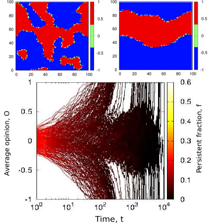
A qualitative idea of the dynamics can be gained by looking at the opinion configurations of the KEM at various stages of the dynamics (see Fig. 1). The snapshots clearly indicate the presence of two time scales. At the initial times (), the spin domain configurations are random. At a later stage (), if the system has not already entered a fully consensus state, it is in a state with two (or more, in principle) large domains (taking the periodic boundary conditions into account).
III.1 System size scaling of the two consensus time scales
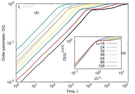
We first study the behavior of the global order parameter given by . The simulations are done on square lattices, with the sizes () indicated in the figures and following periodic boundary conditions. Unless otherwise mentioned, the initial conditions are completely random i.e., equal probability for the three opinion values and . The realization averages are between 10000 to 100, depending on the system sizes. In Fig. 2 we show how the order parameter evolves in time for various system sizes. It is clear from Fig. 2(a) that the evolution shows the effect of the two time scales mentioned earlier. For the initial part of the dynamics, the order parameter increases in a power-law manner with time, with the exponent value about , which is the same as in Ising model coarsening. The growth, however, drastically slows down when the second time scale manifests itself. The subsequent growth is much slower, which continues until complete consensus is reached. The inset of Fig. 2(a) confirms that where is a dynamic exponent of growth. This value of indicates a dynamical evolution which is curvature driven and valid for the zero temperature coarsening of Ising model in all dimensions.
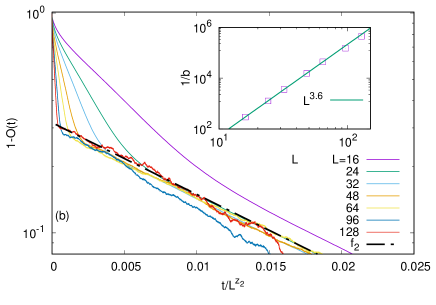
For , the order parameter can be fitted to a functional form
| (2) |
indicating that represents another time scale which we identify as . is shown in the inset of Fig. 2(b) and we find
| (3) |
where . In Fig. 2(b) we obtain a partial collapse of the data for the late time regime using using Eqs (2) and (3).
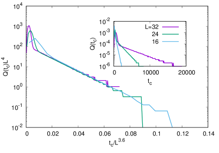
We also obtain the distribution of the consensus times as shown in the inset of Fig. 3. The peak in the distribution function corresponds to the shorter consensus time or domain-wall formation time scale , where the configurations either reach consensus avoiding the domain wall formation or reach the domain-wall states. However, the tail of the distribution, which represents the time scales for the domain walls to merge, i.e., formation of the overall consensus, gives the second, much larger, time scale . One can obtain a collapse of the data for the tail by scaling by . It is also observed that the scaling function has an exponential behavior.
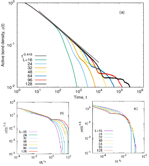
Finally, for the analysis of the two time scales, we look at the active bond density , which is defined as the density of neighboring pairs of agents having different opinion values. This quantity is widely studied in the voter-like models, and shows a power law decay when intermediate states are allowed. We note a power law decay here in the initial stage with an exponent value . The decay then slows down and shows a plateau region which is attributed to the formation of the domain wall states (see Fig. 4), eventually drops to zero, when a consensus is reached. The time scale for reaching the plateau and then the eventual exponential decay should correspond to the two time scales and obtained before. Data collapses in the initial and later stages, obtained using the scaling variables and respectively and shown in Fig. 4, confirm the presence of the two time scales. The collapses improve for larger system sizes.
III.2 Persistence and exit probabilities
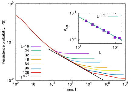
The persistence of the opinion value of a given agent is an interesting measure of the stability of dynamics in a model. In zero temperature quench of Ising model, this is well studied satya-rev . The persistence probability at any time is the fraction of agents who did not change their opinion values at all up to that time. Fig. 5 shows the decay of the persistence probability for the KEM. Although it does not show a clear power law behavior for small system sizes, for the largest size, a power law behavior can be detected over a considerable time range. From this regime, one obtains
| (4) |
with , clearly distinct from that found in the two dimensional Ising model blanch . Furthermore, due to the fact that the dynamics may not be frozen after time , the persistence probability does not become time independent beyond (before reaching a saturation value) as in the case of Ising model. However, the subsequent decay of the persistence probability is, like the growth of the order parameter discussed before, very slow. Hence, the effect of the two time scales described above is also visible in this measure. We also note that the saturation value of varies with as shown in the inset of Fig. 5.
The exit probability is another important measure that quantifies the probability to reach a particular consensus state with an initial bias. In particular, if an initial bias is ineffective (e.g., an initial configuration with more ultimately ends up in an all state) it can be called a case of minority spreading. This is again a very well studied quantity in Ising model and other opinion dynamics models sznajd_exit ; sznajd2 ; lamb ; timp ; parna ; parna1 ; parna2 ; suman . The general scaling form of the exit probability reads
| (5) |
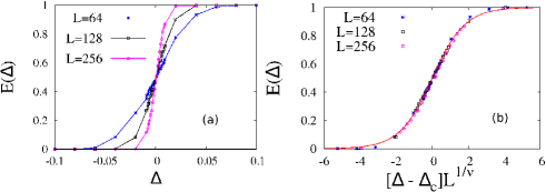
where is the bias in the initial opinion fractions (initial densities are , and for opinion values 0, respectively; ), with and being interpreted as a correlation length exponent (to be distinguished from the critical correlation length). The exit probabilities and their finite size scaling are shown in Fig. 6. The exponent value of for the collapse is which is again distinct from what is seen in the Ising model in two dimensions () pratik2017 . The scaling function can be fit to the form with .
IV Comparison with other dynamical models
The present model, although a three state model, has only two stable fixed points, all +1/ all -1 and hence can be compared with other models studied extensively in the literature. We have in mind precisely the Ising model or voter like models which are special cases of the generalized voter model oliv . We have already mentioned some differences compared to the Ising model, the most important of which is the absence of frozen states at extremely large times. This is attributed to the fact that the zero states are primarily found at the domain boundaries which on interacting with any nonzero opinion is bound to change. So the boundaries of a zero domain naturally recede resulting into a narrowing of the zero band before it vanishes. The vanishing of a zero domain brings into contact domains of opinion thereby again producing some zeroes at their boundary. However, as in any finite system, a random fluctuation will drive the system to either of the all 1 or all -1 state. While the consensus state is reached for all configurations, this kind of slow dynamics to reach the consensus state is seen in about 30 of all the random initial configurations used. Such metastability is possible only in dimensions greater than one, hence in one dimension, dynamics of both Ising model and KEM coincide. It is already known that the voter model dynamics are identical to that of Ising in one dimension, so that all three models show the same dynamical behavior in one dimension.
In the KEM, as discussed before, there are two time scales in the coarsening process, the second being much larger than the first. It is true that in the two dimensional Ising model also, one gets a two time scale scenario due to the slow relaxation of the so called diagonal states b_redner where the scaling of the second time scale is quite similar to what we get. However, such cases were much more rare (nearly 5 of the consensus states) to affect the bulk dynamical behavior compared to KEM where the slow dynamics occur in about cases. In the Ising model, the dynamics are always curvature driven. In the KEM, the initial evolution is perhaps the same indicated by the value of . On the other hand, in the voter model, the dynamics are interfacial noise driven so that it shows a different dynamical behavior in two dimensions. In the KEM, the dynamics are like the voter model only for the zero state which simply copies the state of the interacting agent and in that sense partially interfacial noise driven. Since at a later stage, it is basically the zeros which undergo a change, the dynamics become more and more interfacial noise driven. In the generalized voter model, the interplay of the interfacial noise and curvature driven dynamics was studied recently parna2 which showed crossover from a faster to a slower dynamics due to the presence of metastable states with similar nearly straight-edged domains. It was the interfacial noise which was found to lead the system to consensus in the later stages and one can argue that the same is happening in KEM. In the generalized voter model also, two time scales were detected, however, such a large value of was not indicated in that case. On the other hand, the exponent value obtained in the KEM is quite close to that found in a two state majority rule model chen where also one gets long lived metastable states. In this model, the signature of the slow relaxation was captured by the behaviour of the consensus time distribution from which was obtained by extrapolation in two dimensions. A scaling argument, however, indicated that the value should be equal to 3.
Slow coarsening, where the time scale varies with with an exponent close to 3.6, has also been observed in some voter-like models, where one or more intermediate states exist between the two extreme values of the opinions. These include the model for bilingual dynamics, three or more state voter models etc. migu ; cast ; luca ; volo ; vazquez . In these studies, the intermediate states introduced an effective surface tension in the domain walls, driving the system to a curvature driven state. While the concentration of unlike pairs decays approximately as like in our case (we obtained a value ), the scaling is found by not only considering the consensus time distribution but explicitly from the exponentially slow approach to the consensus state manifested by both and in the later stage only in the present work. Except for some special cases for a four state model in vazquez , where an exponential slow approach of the order parameter in the later stages was noted and was remarked to be unique, such a behaviour has not been reported earlier to the best of our knowledge. Thus we argue that the mechanism in the later stages is interface noise driven in the KEM in contrast to that in the three state language and voter like models where the signature of a two stage process has been reported only from the behaviour of the exponential tail of the consensus time distribution and not from the behaviour of the order parameter relaxation.
It is easily checked that the microscopic dynamics in the KEM is quite different compared to e.g., the three state voter model. For example, in the three state voter model, the probability that a zero becomes 1 is equal to where is the density of the opinion of the four neighbours while in the KEM, it is equal to . In this context, it can be mentioned that for the two state models, a generalised formulation in terms of the transition probabilities involving two parameters has been made oliv . The Ising-Glauber model, which uses an energy minimising dynamics and the voter model, in which the agents simply copy the opinion of a randomly chosen neighbour, correspond to two different points in this two dimensional parameter space. These two have quite distinct dynamical behaviour in two or higher dimensions with respect to coarsening, persistence, freezing probability etc. For three state models, one can, in principle, conceive of a similar generalisation with a presumably larger dimensional parameter space. The KEM and the other voter like models, quite different in terms of their microscopic dynamics, are expected to correspond to reasonably well separated points/regions in this parameter space. Even then, the fact that the KEM and the other three state models all show the slow coarsening behaviour with similar dynamical exponent values, strongly suggests that this particular feature is quite generic. Such is, however, not the case in two state models, where it is meaningful to consider variations in the parameters and see the effect, as was done in parna2 .
In none of the multistate models, results for the scaling of persistence probability or the exit probabilities are available, the two other studies which highlight the present work. We note that the persistence probability in KEM decays with an exponent that has a larger value compared to that in the Ising model. This is presumably because in the initial stages many of the zeros definitely change their state thereby reducing in a rapid manner. However, the dynamics in KEM lasts longer and in the later regime, the persistence probability still decays, albeit much slowly as very few changes in state occur for the first time. In comparison, in the Ising model, the system reaches a steady state much faster and attains a constant value after a time scaling as . On the other hand, the persistence probability decays slower in comparison to the voter model (numerically it is found to be ] krap-comp ) where is a critical dimension for which the dynamics are known to be slow for all configurations. Consistently, the saturation value of the persistence, which signifies the end of the dynamical evolution, comes at a much later stage in KEM. This in turn, affects the scaling form of the persistence probability. In Ising model the saturation value varies as , with manoj_ray , where is the unique dynamical exponent for the Ising model and . But in KEM, the saturation value scales as , which does not satisfy the scaling relation mentioned above for either or , with .
The exit probability in the voter model is known to vary linearly with the bias in all dimensions. This follows from the global conservation of the opinions over all ensemble, also true for the one dimensional Ising model. In two dimensions, the Ising model and the Sznajd model show a behavior similar to what we obtain for the KEM, however, the values of the parameters in the scaled functions for the Ising model are quite different ( and pratik2017 ). Although in the thermodynamic limit, the exit probability assumes a step functional form, for finite sizes, there is evidence of minority spreading as indicated by the presence of the universal scaling function, a feature shared by the Ising model, though in the latter it happens to a lesser extent as the value of is larger.
V Comparisons with data
There are examples of issues that eluded consensus in the society for decades and formed a spontaneous polarization like the domain wall state discussed here. One recent example is the question of the United Kingdom leaving the European Union - commonly referred to as Brexit. This issue has certainly made the UK and EU as a whole, more polarized. From opinion surveys dated back to 1970s data , there seems to be a fluctuating tendency in the opinion values, while no side got overwhelming support. These are qualitative features we also find in the KEM considered here. However, while in the model we can quantify these features with various measures, with the data of opinion surveys on Brexit (or related questions), such quantification is difficult.
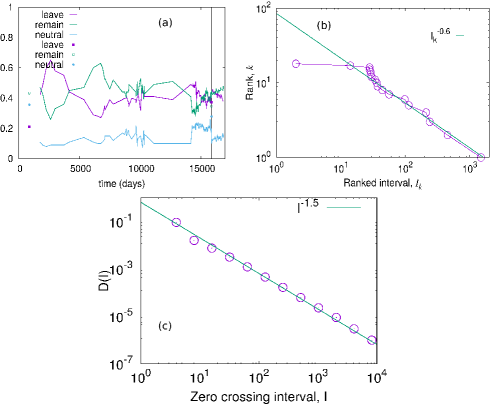
Nevertheless, we can look at the intervals of the so called ‘zero-crossing’ of the overall opinion values, i.e., the intervals in which the majority opinion shifted between “leave” and “remain”. Fig. 7 shows a rank plot of the intervals, which suggests an approximate exponent value of for the cumulative distribution, which in turn suggests as the exponent value for the probability distribution function clauset of the interval of switching of opinions.
For comparison, we considered the time series of the global order parameter of KEM only for the configurations that did not reach consensus in i.e., those configurations which reached a domain-wall state. The distribution of the zero-crossing intervals for those configurations only, gives an exponent value (see Fig. 7), which closely resembles the value suggested from data. However, as noted before, the data available are rather sparse in measurement intervals, which can affect the distribution especially in the lower-cutoff region (not shown). Nevertheless, a manifestation of an active exchange of opinions between two polarized groups is seen in the data that was described in the model.
A possible argument for the origin of the exponent value in the model could be the diffusing motion of the domain walls in effectively one dimension. The exponent is what is seen in the surviving probability for such a walk redner .
VI Discussions and conclusion
Formation of consensus in a multi-agent society has been long viewed as a collective emergent phenomenon. In various models that considers the phenomenon as a critical behavior, in presence of sufficiently weak noise, a majority opinion builds up sen_chak ; galam_book ; def1 . Here we have shown, however, that even in the absence of external noise, formation of opinions can be hindered due to spatial constraint in interactions. Specifically, in the kinetic exchange model of opinion dynamics studied here, we find that for about 30% of realizations, the configuration of opinions in a two-dimensional lattice go to a segregated or domain-wall state, where there are two large groups of opposing opinion values. The groups are, however, not frozen in time. The domain walls move, due to interactions mediated by neutral agents, and eventually merge to form a consensus state. The time-scale to reach the consensus, however, is significantly higher than the time scale for reaching consensus for the non domain-wall states. Indeed, the two time-scales scale differently with system size as well. The scaling of the persistence probability and the overall order parameter quantify these two time scales in the model. This behavior is distinct from other coarsening dynamics, say in two dimensional Ising model, where the domain wall state is frozen in time in absence of external noise.
There are real world scenarios where formation of consensus takes exceptionally long time. It is long seen that in presence of external noise, bounded confidence or zealots, inertial agents etc., formation of consensus could be hindered. But even without such effect, consensus formation could be difficult. We have considered one such case, which is the question of the UK leaving the EU or Brexit. This has seen fragmentation of two groups, none of which could achieve overwhelming support i.e., consensus was not formed. There is a long history of opinion surveys on this question, which shows the fluctuating nature of the two opinion groups. Indeed, in this case there could be external noise, bounded confidence and even zealots, but a simple model could also give the qualitative agreement of the size distribution of the intervals of zero crossing seen in the data and in the model.
In conclusion, we have presented a simple model of kinetic exchange for opinion formation, where two time scales of consensus formation are clearly demonstrated. In about 30% of cases, the model reaches a segregated state, where consensus formation takes a much longer time () than the Ising-like coarsening time-scale (). The persistence behaviour and exit probability have been computed to show distinct departure from the existing results known in two dimensions. We have compared the fluctuating nature of the order parameter around in our model having the meta-stable domain-wall states, with the opinion survey data for Brexit, also fluctuating between leave and remain majorities, to find a possible agreement in the distribution of the zero-crossing intervals.
Acknowledgements: PS acknowledges financial support from SERB scheme EMR/2016/005429 (Government of India).
References
- (1) D. Stauffer, Opinion dynamics and sociophysics, in: R. Meyers (eds) Encyclopedia of Complexity and Systems Science. Springer, New York, NY (2009).
- (2) P. Sen, B. K. Chakrabarti, Sociophysics: An Introduction, Oxford University Press, Oxford (2014).
- (3) C. Castellano, S. Fortunato, V. Loreto, Statistical physics of social dynamics, Rev. Mod. Phys. 81, 591 (2009).
- (4) S. Galam, Sociophysics: A Physicist’s Modeling of Psycho-political Phenomena, Springer, Boston, MA (2012).
- (5) P. Clifford, A. Sudbury, A model for spatial conflict, Biometrika 60, 581 (1973).
- (6) T, M. Liggett, Interacting particle systems, Springer, New York, NY (1985).
- (7) T. M. Liggett, Interacting particle systems: Contact, voter and exclusion processes, Springer-Verlag, Berlin (1999).
- (8) S. Biswas, P. Sen, Critical noise can make the minority candidate win: The US presidential election cases, Phys. Rev. E 96, 032303 (2017).
- (9) G. Deffuant, D. Neau, F. Amblard, G. Weisbuch, Mixing beliefs among interacting agents, Adv. Complex Syst. 3, 87 (2000).
- (10) R. Hegselmann, U. Krause, Opinion dynamics and bounded confidence models, analysis and simulation J. Art. Soc. Soc. Sim. 5, 3 (2002).
- (11) G. Toscani, Kinetic models of opinion formation, Comm. Math. Sci. 4, 481 (2006).
- (12) M. Lallouache, A. S. Chakrabarti, A. Chakraborti, B. K. Chakrabarti, Opinion formation in kinetic exchange models: Spontaneous symmetry breaking transition, Phys. Rev. E 82, 056112 (2010).
- (13) P. Sen, Noise-driven dynamic phase transition in a one-dimensional Ising-like model, Phys. Rev. E 81, 032103 (2010).
- (14) S. Biswas, Mean-field solutions of kinetic-exchange opinion models, Phys. Rev. E 84, 056106 (2011).
- (15) P. Sen, Nonconservative kinetic exchange model of opinion dynamics with randomness and bounded confidence, Phys. Rev. E 86, 016115 (2012).
- (16) S. Biswas, A. Chaterjee, P. Sen, Disorder induced phase transition in kinetic models of opinion formation, Physica A 391, 3257 (2012).
- (17) K. Roy Chowdhury, A. Ghosh, S. Biswas, B. K. Chakrabarti, Kinetic exchange opinion model: solution in the single parameter map limit, in Econophysics of Agent-Based Models, F. Abergel, H. Aoyama, B. K. Chakrabarti, A. Chakraborti, A. Ghosh (eds), New Economic Windows, pp 131-143 (2014).
- (18) C. Brugna, G. Toscani, Kinetic models of opinion formation in the presence of personal conviction, Phys. Rev. E 92, 052818 (2015).
- (19) K. Sznajd-Weron, J. Sznajd, Opinion evolution in closed community, Int. J. Mod. Phys. C 11, 1157 (2000).
- (20) S. Biswas, P. Sen, Model of binary opinion dynamics: Coarsening and effect of disorder, Phys. Rev. E 80, 027101 (2009).
- (21) By consensus we mean that the opinions of all the agents are strictly same ().
- (22) V. Spirin, P. L. Krapivsky, S. Redner, Fate of zero-temperature Ising ferromagnets, Phys. Rev. E 63, 036118 (2001).
- (23) P. Svenson, Freezing in random graph ferromagnets, Phys. Rev. E 64, 036122 (2001).
- (24) O. Häggström, Zero-temperature dynamics for the ferromagnetic Ising model on random graphs, Physica A 310, 275 (2002).
- (25) D. Boyer, O. Miramontes, Interface motion and pinning in small-world networks, Phys. Rev. E 67, R035102 (2003).
- (26) C. Castellano, V. Loreto, A. Barrat, F. Cecconi, D. Parisi, Comparison of voter and Glauber ordering dynamics on networks, Phys. Rev. E 71, 066107 (2005).
- (27) S. Biswas, P. Sen, Effect of the nature of randomness on quenching dynamics of the Ising model on complex networks, Phys. Rev. E 84, 066107 (2011).
- (28) Y. Baek, M. Ha, H. Jeong, Absorbing states of zero-temperature Glauber dynamics in random networks, Phys. Rev. E 85, 031123 (2012).
- (29) A. Khaleque, P. Sen, Frozen states and active-absorbing phase transitions of the Ising model on networks, Journal of Complex Networks 4, 330 (2016).
- (30) E. Ben-Naim, L. Frachebourg, P. L. Krapivsky, Coarsening and persistence in the voter model, Phys. Rev. E 53, 3078 (1996).
- (31) C. Castellano, D. Vilone, A. Vespignani, Incomplete ordering of the voter model on small-world networks, EPL 63, 153 (2003).
- (32) V. Sood, S. Redner, Voter model on heterogeneous graphs, Phys. Rev. Lett. 94, 178701 (2005).
- (33) K. Suchecki, V. M. Eguíluz, M. San Miguel, Voter model dynamics in complex networks: Role of dimensionality, disorder, and degree distribution, Phys. Rev. E 72, 036132 (2005).
- (34) E. Ben-Naim, P. L. Krapivsky, F. Vazquez, S. Redner, Unity and discord in opinion dynamics, Physica A 330, 99 (2003).
- (35) F. Vazquez, P. L. Krapivsky, S. Redner, Constrained opinion dynamics: freezing and slow evolution, J. Phys. A 36, L61 (2003).
- (36) N. Crokidakis, C. Anteneodo, Role of conviction in nonequilibrium models of opinion formation, Phys. Rev. E 86, 061127 (2012).
- (37) N. Crokidakis, Phase transition in kinetic exchange opinion models with independence, Phys. Lett. A 378, 1683 (2014).
- (38) S. Mukherjee, A. Chatterjee, Disorder-induced phase transition in an opinion dynamics model: Results in two and three dimensions, Phys. Rev. E 94, 062317 (2016).
- (39) F. W. S. Lima, J. A. Plascak, Kinetic models of discrete opinion dynamics on directed Barabasi-Albert networks, Entropy 2019, 942 (2019).
- (40) X. Castelló, V. M. Eguíluz and M. San Miguel, Ordering dynamics with two non-excluding options: bilingualism in language competition, New Journal of Physics 8, 308 (2006).
- (41) X. Castelló, A. Baronchelli, V. Loreto, Consensus and ordering in language dynamics, Eur. Phys. J. B 71, 557 (2009).
- (42) L. Dall’Asta and T. Galla, Algebraic coarsening in voter models with intermediate states, Journal of Physics A: Mathematical and Theoretical, 41, 435003 (2008).
- (43) D. Volovik and S. Redner, Dynamics of confident voting, J. Stat. Mech: Theory and Experiment, P04003 (2012).
- (44) F. Velásquez-Rojas, F. Vazquez, Opinion dynamics in two dimensions: domain coarsening leads to stable bi-polarization and anomalous scaling exponents, J. Stat. Mech: Theory and Experiment, 043403 (2018).
- (45) The code used in this work is available at: https://github.com/soumya-84/KEMmodel2d
- (46) A. J. Bray, S. N. Majumdar, G. Schehr, Persistence and first-passage properties in nonequilibrium systems, Adv. Phys. 62, 225 (2013).
- (47) T. Blanchard, L. F. Cugliandolo, M. Picco, Persistence in the two dimensional ferromagnetic Ising model, J. Stat. Mech. 2014, P12021 (2014).
- (48) S. Galam, Opinion dynamics, minority spreading and heterogeneous beliefs in Econophysics and Sociophysics: Trends and Perspectives, Chap. 13, Wiley-VCH Verlag, B. K. Chakrabarti, A. Chakraborti, A. Chaterjee (eds) (2006).
- (49) D. Stauffer, Monte Carlo simulations of Sznajd models, Journal of Artificial Societies and Social Simulation 5, no. 1, paper 4 ¡http://jasss.soc.surrey.ac.uk/5/1/4.html¿ (2002).
- (50) F. Slanina, K. Sznajd-Weron, P. Przybyla, Some new results on one-dimensional outflow dynamics, Europhysics Letters 82, 18006 (2008).
- (51) R. Lambiotte, S. Redner, Dynamics of non-conservative voters, Europhysics Letters 82, 18007 (2008).
- (52) A. M. Timpanaro, S. Galam, On the exit probability of the extended Sznajd model and the Kirkwood approximation, J. Phys.: Conf. Ser. 633 012111 (2015).
- (53) P. Roy, P. Sen, Exit probability in generalized kinetic Ising model, J. Stat. Phys. 159, 893 (2015).
- (54) P. Roy, S. Biswas, P. Sen, Exit probability in inflow dynamics: Nonuniversality induced by range, asymmetry and fluctuation, Phys. Rev. E 89, 030103 (2014).
- (55) P. Roy, P. Sen, Interplay of interfacial noise and curvature driven dynamics in two dimensions, Phys. Rev. E 95, 020101(R) (2017).
- (56) S. Biswas, S. Sinha, P. Sen, Opinion dynamics model with weighted influence: Exit probability and dynamics, Phys. Rev. E 88, 022152 (2013).
- (57) P. Mullick, P. Sen, Zero-temperature coarsening in the Ising model with asymmetric second-neighbor interactions in two dimensions, Phys. Rev. E 95, 052150 (2017).
- (58) M. J. de Oliveira, J. F. F. Mendes, M. A. Santos, Nonequilibrium spin models with Ising universal behaviour, J. Phys. A: Math. Gen. 26, 2317 (1993).
- (59) P. Chen, S. Redner. Majority Rule Dynamics in Finite Dimensions, Phys. Rev. E 71, 036101 (2005).
- (60) G. Manoj, P. Ray, Scaling and fractal formation in persistence, J. Phys. A 33, L109 (2000).
- (61) The survey data can be found here: https://www.ipsos.com/ipsos-mori/en-uk/european-union-membership-trends
- (62) A. Clauset, C. R. Shalizi, M. E. J. Newman, Power-law Distributions in Emperical Data, SIAM Review 51, 661 (2009).
- (63) S. Redner, A guide to first passage processes, Cambridge University Press, 2001.