[2001.11950] 1 Introduction

Non-reversibly updating a uniform $[0,1]$ value
for Metropolis accept/reject decisions¹¹1An earlier version of this work was presented at the 2nd Symposium on Advances in Approximate Bayesian Inference, Vancouver, British Columbia, 8 December 2019.

Radford M. Neal²²2 Dept. of Statistical Sciences and Dept. of Computer Science, University of Toronto, Vector Institute Affiliate. http://www.cs.utoronto.ca/ $\sim$ radford/, radford@stat.utoronto.ca
31 January 2020

Abstract. I show how it can be beneficial to express Metropolis accept/reject decisions in terms of comparison with a uniform $[0,1]$ value, $u$ , and to then update $u$ non-reversibly, as part of the Markov chain state, rather than sampling it independently each iteration. This provides a small improvement for random walk Metropolis and Langevin updates in high dimensions. It produces a larger improvement when using Langevin updates with persistent momentum, giving performance comparable to that of Hamiltonian Monte Carlo (HMC) with long trajectories. This is of significance when some variables are updated by other methods, since if HMC is used, these updates can be done only between trajectories, whereas they can be done more often with Langevin updates. I demonstrate that for a problem with some continuous variables, updated by HMC or Langevin updates, and also discrete variables, updated by Gibbs sampling between updates of the continuous variables, Langevin with persistent momentum and non-reversible updates to $u$ samples nearly a factor of two more efficiently than HMC. Benefits are also seen for a Bayesian neural network model in which hyperparameters are updated by Gibbs sampling.

1 Introduction

In the Metropolis MCMC method, a decision to accept or reject a proposal to move from $x$ to $x^{*}$ can be done by checking whether $u<\pi(x^{*})/\pi(x)$ , where $\pi$ is the density function for the distribution being sampled, and $u$ is a uniform $[0,1]$ random variable. Standard practice is to generate a value for $u$ independently for each decision. I show here that it can be beneficial to instead update $u$ each iteration without completely forgetting the previous value, using a non-reversible method.

Doing non-reversible updates to $u$ will not change the fraction of proposals that are accepted, but can result in acceptances being clustered together (with rejections similarly clustered). This can be beneficial, for example, when rejections cause reversals of direction, as in Horowitz’s (1991) variant of Langevin updates for continuous variables in which the momentum “persists” between updates. Compared to the alternative of Hamiltonian Monte Carlo (HMC) with long trajectories (Duane, Kennedy, Pendleton, and Roweth 1987; reviewed in Neal 2011), Langevin updates allow other updates, such as for discrete variables, to be done more often, which I will show can produce an advantage over HMC if persistent momentum is used in conjunction with non-reversible updates for $u$ .

2 The New Method for Accept/Reject Decisions

For any MCMC method, we can augment the variable of interest, $x$ , with density $\pi(x)$ , by a variable $s$ , whose conditional distribution given $x$ is uniform over $[0,\pi(x)]$ . The resulting joint distribution for $x$ and $s$ is uniform over the region where $0<s<\pi(x)$ . This is the view underlying “slice sampling” (Neal 2003), in which $s$ is introduced temporarily, by sampling uniformly from $[0,\pi(x)]$ , and then forgotten once a new $x$ has been chosen. Metropolis updates can also be viewed in this way, with the new $x$ found by accepting or rejecting a proposal, $x^{*}$ , according to whether $\pi(x^{*})>s$ , with $s$ newly sampled from $[0,\pi(x)]$ .

However, it is valid to instead retain $s$ in the state between updates, utilizing its current value for accept/reject decisions, and updating this value when desired by any method that leaves invariant the uniform distribution on $[0,\pi(x)]$ , which is the conditional distribution for $s$ given $x$ implied by the uniform distribution over $(x,s)$ for which $0<s<\pi(x)$ .

Equivalently, one can retain in the state a value $u$ whose distribution is uniform over $[0,1]$ , independent of $x$ , with $u$ corresponding to $s/\pi(x)$ — the state $(x,u)$ is just another way of viewing the state $(x,s)$ . Accept/reject decisions are then made by checking whether $u<\pi(x^{*})/\pi(x)$ . Note, however, that if $x^{*}$ is accepted, $u$ must then be updated to $u\,\pi(x)/\pi(x^{*})$ , which corresponds to $s$ not changing.

Here, I will consider non-reversible updates for $u$ , which translate it by some fixed amount, $\delta$ , and perhaps add some noise, reflecting off the boundaries at $0$ and $1$ . It is convenient to express such an update with reflection in terms of a variable $v$ that is uniform over $[-1,+1]$ , and define $u=|v|$ . An update for $v$ can then be done as follows:

	$\displaystyle v\ \leftarrow\ v\ +\ \delta\ +\ \mbox{noise}$
	$\displaystyle\mbox{while\ }v>+1:\ \ v\ \leftarrow\ v-2$				(1)
	$\displaystyle\mbox{while\ }v<-1:\ \ v\ \leftarrow\ v+2$

For any $\delta$ and any distribution for the noise (not depending on the current value of $v$ ), this update leaves the uniform distribution over $[-1,+1]$ invariant, since it is simply a wrapped translation, which has Jacobian of magnitude one, and hence keeps the probability density for the new $v$ the same as the old $v$ (both being $1/2$ ).

The full state consists of $x$ and $v$ , with $x$ having density $\pi(x)$ and, independently, $v$ being uniform over $[-1,+1]$ , which corresponds to the conditional distribution (given $x$ ) of $s=|v|\pi(x)$ being uniform over $[0,\pi(x)]$ . If a proposed move from $x$ to $x^{*}$ is accepted we must change $v$ as follows:

\displaystyle v

\displaystyle\leftarrow

\displaystyle v\,\pi(x)/\pi(x^{*})

(2)

This leaves $s$ unchanged, and hence the reverse move would also be accepted, as necessary for reversibility. Because of this change to $v$ on acceptance, when $\pi(x)$ varies continuously, it may not be necessary to include noise in the update for $v$ in (1), but if $\pi(x)$ has only a finite number of possible values, adding noise may be necessary to ensure ergodicity.

The hope with these non-reversible updates is that $u$ will move slowly (if $\delta$ and the noise amount are small) between values near 0, where acceptance is easy, and values near 1, where acceptance is harder. (But note that $u$ may change in either direction when proposals are accepted, though $s$ will not change.) Non-reversibly updating $u$ will not change the overall acceptance rate, since the distribution of $u$ is still uniform over $[0,1]$ , independent of $x$ , but it is expected that acceptances and rejections will become more clustered — with an accepted proposal more likely to be followed by another acceptance, and a rejected proposal more likely to be followed by another rejection.

We might wish to intermingle Metropolis updates for $x$ that use $v$ to decide on acceptance with other sorts of updates for $x$ — for example, Gibbs sampling updates, or Metropolis updates accepted in the standard fashion. We can do these updates while ignoring $v$ , and then simply resume use of $v$ afterwards, since $v$ is independent of $x$ . We could indeed include several independent $v$ variables in the state, using different $v$ values for different classes of updates, but this generalization is not explored here.

3 Results for random-walk Metropolis updates in high dimensions

A small benefit from non-reversible updating of $u$ can be seen with simple random-walk Metropolis updates. Such updates operate as follows:

1)

Propose $x^{*}\sim N(x,\sigma^{2}I)$ , where $\sigma$ is a stepsize parameter that needs to be tuned.
2)

Accept $x^{\prime}=x^{*}$ as next state if $u<\pi(x^{*})/\pi(x)$ ,; otherwise let $x^{\prime}=x$ .

Figure 1 compares results of such updates when $u$ is sampled independently each iteration versus being updated non-reversibly as described in Section 2, when sampling a 40-dimensional Gaussian distribution with identity covariance matrix. When estimating the mean of a single coordinate, little difference is seen, but for estimating the mean of the log of the probability density, the non-reversible method with $\delta=0.3$ is $3.47/3.03\approx 1.15$ times better.

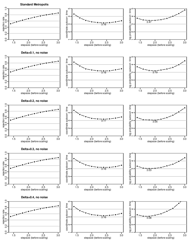
Refer to caption — Figure 1: Sampling from a 40-dimensional Gaussian with identity covariance. The values for $\sigma$ used were the stepsizes shown above divided by $40^{1/2}$ . The autocorrelation times (one plus twice the sum of autocorrelations at lags 1 to when they are negligible) that are shown are for groups of 40 iterations (hence the single-iteration autocorrelation time is about 40 times larger). Results are shown for standard Metropolis, and for Metropolis with non-reversible update for $u$ , with $\delta=0.1,0.2,0.3,0.4$ , and no noise.

One possible explanation for the better performance with non-reversible updates is that, as noted by Caracciolo, et al (1994), the performance of Metropolis methods in high dimensions is limited by their ability to sample different values for the log of the density. In $D$ dimensions, the log density typically varies over a range proportional to $D^{1/2}$ . A Metropolis update will typically change the log density only by about one — larger decreases in the log density are unlikely to be accepted, and it follows from reversibility that increases in the log density of much more than one must also be rare (once equilibrium has been reached). Since standard Metropolis methods are reversible, these changes of order one will occur in a random walk, and so around $D$ steps will be needed to traverse the range of log densities of about $D^{1/2}$ , limiting the speed of mixing.

The gain seen from using non-reversible updates for $u$ may come from helping with this problem. When $u$ is small few proposals will be rejected, and the chain will tend to drift towards smaller values for the log density, with the opposite behaviour at times when $u$ is near one. This could reduce the random walk nature of changes in the log density. Note, however, that this effect is limited by the changes to $v$ (and hence $u$ ) required by equation (2).

4 Application to Langevin updates with persistent momentum

I obtained more interesting results when using non-reversible updates of $u$ in conjunction with the one-step, non-reversible version of Hamiltonian Monte Carlo (Duane, et al 1987) due to Horowitz (1991). This method is a form of “Langevin” update in which the momentum is only partially replaced in each iteration, so that the method tends to move persistently in the same direction for many iterations. I briefly present this method below; it is discussed in more detail in my review of Hamiltonian Monte Carlo methods (Neal 2011, Section 5.3).

Hamiltonian Monte Carlo (HMC) works in a state space extended with momentum variables, $p$ , of the same dimension as $x$ , which are newly sampled each iteration. The distribution for $x$ is defined in terms of a “potential energy” function $U(x)$ , with $\pi(x)\propto\exp(-U(x))$ . HMC proposes a new value for $(x,p)$ by simulating Hamiltonian dynamics with some number of “leapfrog” steps (and then negating $p$ , so the proposal is reversible). A leapfrog step from $(x_{t},p_{t})$ to $(x_{t+\eta},p_{t+\eta})$ has the form

$\displaystyle p_{t+\eta/2}$	$\displaystyle=$	$\displaystyle p_{t}\ -\ (\eta/2)\,\nabla U(x_{t})$
$\displaystyle x_{t+\eta}$	$\displaystyle=$	$\displaystyle x_{t}\ +\ \eta\,p_{t+\eta/2}$	(3)
$\displaystyle p_{t+\eta}$	$\displaystyle=$	$\displaystyle p_{t+\eta/2}\ -\ (\eta/2)\,\nabla U(x_{t+\eta})\vspace{-4pt}$

$L$ such steps may be done to go from the current state $(x,p)=(x_{0},p_{0})$ to the proposal $(x^{*},p^{*})=(x_{\eta L},-p_{\eta L})$ . If $\eta L$ is large, but $\eta$ is sufficiently small (so acceptance is likely), a proposed point can be accepted that is distant from the current point, avoiding the slowdown from doing a random walk with small steps. In standard HMC, $p$ is sampled independently at each iteration from the $N(0,I)$ distribution, randomizing the direction in which the next trajectory starts out.

The standard Langevin method is equivalent to HMC with $L=1$ . This method makes use of gradient information, $\nabla U(x)$ , which gives it an advantage over simple random-walk Metropolis methods, but it does not suppress random walks, since $p$ is randomized after each step.

In Horowitz’s method, only one leapfrog step is done each iteration, as for standard Langevin updates, but a trick is used so that these steps nevertheless usually keep going in the same direction for many iterations, except on a rejection. The updates with this method operate as follows:

1)

Set $p^{\prime}=\alpha p\ +\,\sqrt{1\!-\!\alpha^{2}}\,n$ , where $n\sim N(0,I)$ , and $\alpha$ is a tuning parameter. Set $x^{\prime}=x$ .
2)

Find $(x^{*}\!,p^{*})$ from $(x^{\prime}\!,p^{\prime})$ with one leapfrog step, with stepsize $\eta$ , followed by negation of $p$ .
3)

Accept $(x^{\prime\prime},\!p^{\prime\prime})=(x^{*}\!,p^{*})$ if $u\ <\ \pi(x^{*}\!,p^{*})/\pi(x^{\prime}\!,p^{\prime})$ ; otherwise $(x^{\prime\prime}\!,p^{\prime\prime})=(x^{\prime}\!,p^{\prime})$ .
4)

Let $p^{\prime\prime\prime}=-p^{\prime\prime}$ and $x^{\prime\prime\prime}=x^{\prime\prime}$ .

For $\alpha$ slightly less than 1, Step (1) only slightly changes $p$ . If Step (3) accepts, the negation in the proposal is canceled by the negation in Step (4). But a rejection will reverse $p$ , leading the chain to almost double back on itself. Setting $\alpha$ to zero gives the equivalent of the standard Langevin method.

Unfortunately, even with this non-reversibility trick, and an optimally-chosen $\alpha$ , Horowitz’s method is not as efficient as HMC with long trajectories. To reduce the rejection rate, and hence random-walk-inducing reversals of direction, a small, inefficient stepsize ( $\eta$ ) is needed.

But a higher rejection rate would be tolerable if rejections cluster in time, producing long runs of no rejections. For example, rejection-free runs of 20, 0, 20, 0, …are better than rejection-free runs of 10, 10, 10, 10, …, since $N$ of the former runs will potentially move via a random walk a distance proportional to $20(N/2)^{1/2}\,\approx\,14\,N^{1/2}$ , whereas $N$ of the latter runs will move only a distance proportional to $10\,N^{1/2}$ .

We may hope that such clustering of rejections will be obtainable using non-reversible updates of $u$ , with consequent improvement in the performance of Langevin with persistent momentum.³³3Non-reversible updates of $u$ can also benefit the standard Langevin method. In particular, when sampling from the 40-dimensional Gaussian of Section 3, using non-reversible updates of $u$ (with $\delta=0.7$ ) results in a factor of 1.19 lower autocorrelation time for the log probability density compared to the standard Langevin method.

5 Results for Langevin updates with persistent momentum

To test whether non-reversible updating of $u$ can improve the Langevin method with persistent momentum, I first tried sampling a multivariate Gaussian distribution consisting of 16 independent pairs of variables having variances of 1 and correlations of 0.99 (i.e., a 32-dimensional Gaussian with block-diagonal covariance matrix). For this test, the methods are not set up to use knowledge of this correlation structure, mimicking problems in which the dependencies take a more complex, and unknown, form.

The high correlation within each pair and (moderately) high dimensionality limit the stepsize ( $\eta$ ) that can be used (while avoiding a high rejection rate). This test is therefore representative of problems in which sampling is much more efficient when many consecutive small steps to go in the same direction, rather than doing a random walk.

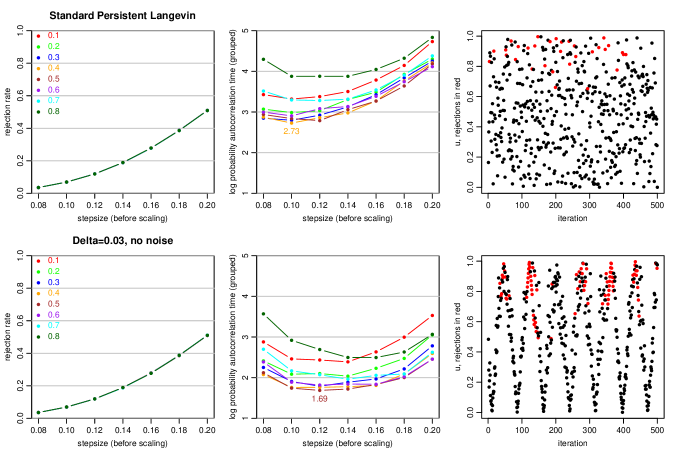
Figure 2 shows the results. The centre plots show that the run using a non-reversible update for $u$ (with $\delta=0.03$ , $\eta=0.12/32^{1/6}=0.0673$ , and $\alpha=0.5^{\eta}=0.954$ ) is $2.73/1.69\approx 1.62$ times better at estimating the mean of the log probability density than the best run of the standard persistent Langevin method (with $\eta=0.10/32^{1/6}=0.0561$ and $\alpha=0.4^{\eta}=0.950$ ). The right plots show that rejections are indeed clustered when non-reversible updates are used, which reduces random walks.

For comparison, I tried HMC for this problem, with stepsizes of $\eta=0.04,0.05,\ldots,0.14,0.15$ and trajectories with the number of leapfrog steps being $L=1,2,4,8,16,32$ . The autocorrelation time for the log probability density was found for groups of $32/L$ HMC updates, giving results that are roughly comparable to those shown in Figure 2. The best performance was for $L=16$ and $\eta=0.07$ , for which the autocorrelation time was 2.04 (though it’s possible that better results might be found with a search over a finer grid for $L$ ). This is worse than the best result of 1.69 for persistent Langevin with non-reversible updates of $u$ , using the stepsize of $0.12/32^{1/6}=0.0673$ , which interestingly is close to the optimal stepsize for HMC. Use of a non-reversible update for $u$ has allowed persistent Langevin to match or exceed the performance of HMC for this problem.

I also used these methods to sample from a mixed continuous/discrete distribution, which may be specified as follows (with variables being conditionally independent except as shown):

$\displaystyle u$	$\displaystyle\sim$	$\displaystyle N(0,1)$
$\displaystyle v\ \|\ u$	$\displaystyle\sim$	$\displaystyle N(u,\,0.04^{2})$
$\displaystyle w_{1}\ \|\ u$	$\displaystyle\sim$	$\displaystyle\mbox{Bernoulli\,}(1/(1+e^{u}))$
	$\displaystyle\vdots$
$\displaystyle w_{20}\ \|\ u$	$\displaystyle\sim$	$\displaystyle\mbox{Bernoulli\,}(1/(1+e^{u}))$

This distribution is intended to mimic more complex distributions having both continuous and discrete variables, which are dependent. I will consider only MCMC methods that alternate updates for the continuous variables, $u$ and $v$ , with updates for the binary variables, $w_{1},\ldots,w_{20}$ (by Gibbs sampling).

Since the marginal distribution of $u$ is known to be $N(0,1)$ , the quality of the sampling for $u$ is easily checked. Because of the high dependence between $u$ and the 20 binary variables, we might expect that a method that frequently updates both the continuous and the binary variables will do better than a method, such as HMC with long trajectories, in which the binary variables are updated infrequently — i.e., only after substantial computation time is spent updating the continuous variables.

In assessing performance, I assume that computation time is dominated by updates of the continuous variables, which in a real application would be more numerous, and in particular by evaluation of their log density, conditional on the current values of the binary variables. (This is not always actually the case here, however, due to the problem simplicity and to avoidable inefficiencies in the software used.)

I tried HMC with trajectories of 30, 40, or 60 leapfrog steps ( $L$ ), and stepsize ( $\eta$ ) of 0.025, 0.030, 0.035, 0.040, and 0.045. Gibbs sampling updates were done between trajectories. Autocorrelation times were found for a group of $120/L$ HMC trajectories. Persistent Langevin with non-reversible updates of $u$ was tried with $\delta$ of 0.003, 0.005, 0.010, and 0.015, each with all combinations of $\alpha$ in 0.98, 0.99, 0.995, 0.9975, 0.9985, and 0.9990 and $\eta$ in 0.015, 0.020, 0.025, 0.030, 0.040, and 0.050. Gibbs sampling updates were done after every tenth update. Autocorrelation times were found for a group of 60 Langevin updates — note that this involves half as many log density gradient evaluations as for a group of HMC iterations.

Performance was evaluated in terms of estimating the mean of the indicator for $u$ being in $(-0.5,1.5)$ . Autocorrelation time for this function was minimized for HMC with $L=40$ and $\eta=0.035$ , with the minimum being 1.53. Autocorrelation time was minimized for persistent Langevin with non-reversible updates of $u$ with $\delta=0.010$ , $\alpha=0.995$ , and $\eta=0.030$ , with the minimum being 1.67. Considering that the HMC groups require twice as many gradient evaluations, persistent Langevin with non-reversible updates of $u$ is $2\times 1.53\,/\,1.67=1.83$ times more efficient than HMC for this problem.

6 Use for Bayesian neural networks

I have also tried using the persistent Langevin method with non-reversible updates for $u$ to sample the posterior distribution of a Bayesian neural network model. Such models (Neal 1995) typically have hyperparameters controlling the variance of groups of weights in the network. It is convenient to use Gibbs sampling updates for these hyperparameters, alternating such updates with HMC updates for the network weights. However, when long trajectories are used for HMC, as is desirable to reduce random-walk behaviour, the Gibbs sampling updates for hyperparameters are done infrequently. Using persistent Langevin updates for weights would allow hyperparameters to be updated more frequently, perhaps speeding overall convergence. We may hope that this will work better with a non-reversible update for $u$ .

I tested this approach on a binary classification problem, with 5 inputs, and 300 training cases. A network with one hidden layer of 12 tanh hidden units was used. Only two of the inputs for this problem were relevant, with two more being slightly noisy versions of the two relevant inputs, and one input being independent noise. Five separate hyperparameters controlled the variances of weights out of each input.

For the best-tuned persistent Langevin method with non-reversibe update of $u$ , the average autocorrelation time for the four plausibly-relevant input hyperparameters was 1.25 times smaller than for the best-tuned HMC method. This is an encouraging preliminary result, but tests with more complex networks are needed to assess how much Bayesian neural network training can be improved in this way.

7 References

: Caracciolo, S, Pelisseto, A, and Sokal, A. D. (1994) “A general limitation on Monte Carlo algorithms of Metropolis type”, Physical Review Letters, vol. 72, pp. 179-182. Also available at arxiv.org/abs/hep-lat/9307021
: Duane, S., Kennedy, A. D., Pendleton, B. J., and Roweth, D. (1987) “Hybrid Monte Carlo”, Physics Letters B, vol. 195, pp. 216-222.
: Horowitz, A. M. (1991) “A generalized guided Monte Carlo algorithm”, Physics Letters B, vol. 268, pp. 247-252.
: Neal, R. M. (2003) “Slice sampling” (with discussion), Annals of Statistics, vol. 31, pp. 705-767.
: Neal, R. M. (2011) “MCMC using Hamiltonian dynamics”, in the Handbook of Markov Chain Monte Carlo, S. Brooks, A. Gelman, G. L. Jones, and X.-L. Meng (editors), Chapman & Hall / CRC Press, pp. 113-162. Also available at arxiv.org/abs/1206.1901
: Neal, R. M. (1995) Bayesian Learning for Neural Networks, Ph.D. Thesis, Dept. of Computer Science, University of Toronto, 195 pages.

Appendix — Scripts used to produce results

The experimental results reported were obtained using my Software for Flexible Bayesian Modeling (FBM, the release of 2020-01-24), available at www.cs.utoronto.ca/ $\sim$ radford/fbm.software.html or at gitlab.com/radfordneal/fbm. This software takes the form of a number of programs that are run using Unix/Linux bash shell scripts. Here, I will show scripts that can be used to produce single points in the figures, omitting the more complex scripts and programs used to run the methods with multiple parameter settings and plot the results.

Scripts for random-walk Metropolis in high dimensions

For Figure 1, the following commands may be used to produce the results for standard Metropolis sampling with stepsize of 1.8 (before scaling):

        dim=40
        stepunscaled=1.8
        step=‘calc "$stepunscaled/Sqrt($dim)"‘
        len=1001000

        echo "STANDARD METROPOLIS"

        log=fig-met.log
        bvg-spec $log 1 1 0 ‘calc $dim/2‘
        mc-spec $log repeat $dim metropolis $step
        bvg-mc $log $len

        echo -n "Rejection Rate: "
        bvg-tbl r $log 1001: | series m | tail -1 | sed "s/.*mean://"
        echo -n "Autocorrelation time for coordinate: "
        bvg-tbl q1 $log 1001: | series mvsac 10 0 | tail -1 | sed "s/.* //"
        echo -n "Autocorrelation time for log prob: "
        bvg-tbl E $log 1001: | series mvsac 10 ‘calc $dim/2‘ | tail -1 | sed "s/.* //"