Extremal parameters and their duals for Fuchsian boundary maps

Abstract.

We describe arithmetic cross-sections for geodesic flow on compact surfaces of constant negative curvature using generalized Bowen-Series boundary maps and their natural extensions associated to cocompact torsion-free Fuchsian groups. If the boundary map parameters are extremal, that is, each is an endpoint of a geodesic that extends a side of the fundamental polygon, then the natural extension map has a domain with finite rectangular structure, and the associated arithmetic cross-section is parametrized by this set. This construction allows us to represent the geodesic flow as a special flow over a symbolic system of coding sequences. Moreover, each extremal parameter has a corresponding dual parameter choice such that the “past” of the arithmetic code of a geodesic is the “future” for the code using the dual parameter. This duality was observed for two classical parameter choices by Adler and Flatto; here we show constructively that every extremal parameter set has a dual.

1. Introduction

Any closed, oriented, compact surface $M$ of genus $g\geq 2$ and constant negative curvature can be modeled as a quotient $M=\Gamma\backslash{\mathbb{D}}$, where ${\mathbb{D}}=\left\{\,z\in{\mathbb{C}}:\left|z\right|<1\,\right\}$ is the unit disk endowed with hyperbolic metric

$$\frac{2\left|dz\right|}{1-{\left|z\right|}^{2}}$$

and $\Gamma$ is a finitely generated Fuchsian group of the first kind acting freely on ${\mathbb{D}}$.

Geodesics in this model are half-circles or diameters orthogonal to ${\mathbb{S}}=\partial{\mathbb{D}}$, the circle at infinity. The geodesic flow $\{\widetilde{\varphi}^{t}\}$ on ${\mathbb{D}}$ is defined as an ${\mathbb{R}}$-action on the unit tangent bundle $S{\mathbb{D}}$ that moves a tangent vector along the geodesic defined by this vector with unit speed. The geodesic flow $\{\widetilde{\varphi}^{t}\}$ on ${\mathbb{D}}$ descends to the geodesic flow $\{\varphi^{t}\}$ on the factor $M=\Gamma\backslash{\mathbb{D}}$ via the canonical projection

$$\pi:S{\mathbb{D}}\to SM$$ (1)

of the unit tangent bundles. The orbits of the geodesic flow $\{\varphi^{t}\}$ are oriented geodesics on $M$.

A surface $M=\Gamma\backslash{\mathbb{D}}$ of genus $g$ admits an $(8g-4)$-sided fundamental polygon ${\mathcal{F}}$ (see Figure 1) whose sides satisfy the extension condition of Bowen and Series [7]: the geodesic extensions of these segments never intersect the interior of the tiling sets $\gamma{\mathcal{F}}$, $\gamma\in\Gamma$. We label the sides of ${\mathcal{F}}$ in a counterclockwise order by numbers $1\leq i\leq 8g-4$ and label the vertices of ${\mathcal{F}}$ by $V_{i}$ so that side $i$ connects $V_{i}$ to $V_{i+1}$, with indices mod $8g-4$.

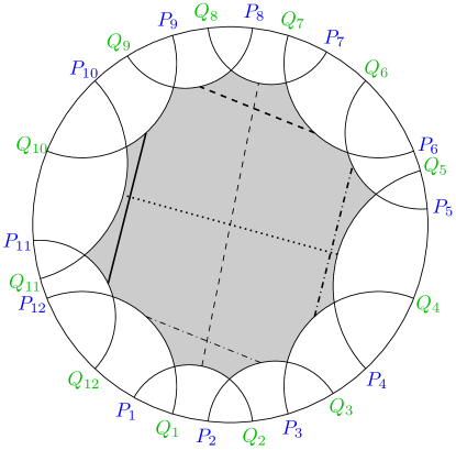
Figure 1. An irregular polygon with side identifications, genus $2$.

We denote by $P_{i}$ and $Q_{i+1}$ the endpoints of the oriented infinite geodesic that extends side $i$ to the circle at infinity ${\mathbb{S}}$. The order of endpoints on ${\mathbb{S}}$ is the following:

$$P_{1},Q_{1},P_{2},Q_{2},\ldots,P_{8g-4},Q_{8g-4}.$$

The identification of the sides of ${\mathcal{F}}$ is given by the side pairing rule

$$\sigma(i):=\left\{\begin{array}[]{ll}4g-i\bmod(8g-4)&\text{ if $i$ is odd}\\ 2-i\bmod(8g-4)&\text{ if $i$ is even}.\end{array}\right.$$ (2)

The generators $T_{i}$ of $\Gamma$ associated to this fundamental domain are Möbius transformations satisfying the following properties, with $\rho(i)=\sigma(i)+1$:

$$T_{i}(V_{i}) =V_{\rho(i)}$$

$$T_{\sigma(i)}T_{i} =\mathrm{Id}$$

$$T_{\rho^{3}(i)}T_{\rho^{2}(i)}T_{\rho(i)}T_{i} =\mathrm{Id}.$$

According to B. Weiss [15], the existence of such a fundamental polygon is an old result of Dehn, Fenchel, and Nielsen, while J. Birman and C. Series [5] attribute it to Koebe [14]. Adler and Flatto [4, Appendix A] give a careful proof of existence and properties of the fundamental $(8g-4)$-gon for any surface group $\Gamma$ such that $\Gamma\backslash{\mathbb{D}}$ is a compact surface of genus $g$. Note that in general the polygon ${\mathcal{F}}$ need not be regular. If ${\mathcal{F}}$ is regular, it is the Ford fundamental domain, i.e., $P_{i}Q_{i+1}$ is the isometric circle for $T_{i}$, and $T_{i}(P_{i}Q_{i+1})=Q_{\sigma(i)+1}P_{\sigma(i)}$ is the isometric circle for $T_{\sigma(i)}$ so that the inside of the former circle is mapped to the outside of the latter, and all internal angles of ${\mathcal{F}}$ are equal to $\pi/2$.

A cross-section $C$ for the geodesic flow $\{\varphi^{t}\}$ is a subset of the unit tangent bundle $SM$ visited by (almost) every geodesic infinitely often both in the future and in the past. It is well-known that the geodesic flow can be represented as a special flow on the space

$${C}^{h}=\{\,(v,s):v\in C,0\leq s\leq h(v)\,\}.$$

It is given by the formula $\varphi^{t}(v,s)=(v,s+t)$ with the identification $(v,h(v))=(R(v),0)$, where the ceiling function $h:C\to{\mathbb{R}}$ is the time of the first return of the geodesic defined by $v$ to $C$, and $R:C\to C$ given by $R(v)=\varphi^{h(v)}(v)$ is the first return map.

Let $\mathcal{A}$ be a finite or countable alphabet, ${\mathcal{A}}^{{\mathbb{Z}}}$ be the space of all bi-infinite sequences $\overline{x}=\{x_{i}\}_{i\in{\mathbb{Z}}}$ with topology induced by the metric $d(\overline{x},\overline{y})=2^{-\!\min\{\left|i\right|:x_{i}\neq y_{i}\}}$. Let $\sigma:{\mathcal{A}}^{\mathbb{Z}}\to{\mathcal{A}}^{\mathbb{Z}}$ be the left shift $(\sigma{\overline{x}})_{i}=x_{i+1}$, and $\Lambda\subset{\mathcal{A}}^{\mathbb{Z}}$ be a closed $\sigma$-invariant subset. Then $(\Lambda,\sigma)$ is called a symbolic dynamical system. There are some important classes of such dynamical systems. The space $({\mathcal{A}}^{\mathbb{Z}},\sigma)$ is called the full shift. If the space $\Lambda$ is given by a set of simple transition rules which can be described with the help of a matrix consisting of zeros and ones, we say that $(\Lambda,\sigma)$ is a subshift of finite type or a one-step topological Markov chain or just a topological Markov chain. A factor of a topological Markov chain is called a sofic shift. For exact definitions, see [8, Section 1.9].

In order to represent the geodesic flow as a special flow over a symbolic dynamical system, one needs to choose an appropriate cross-section $C$ and code it, i.e., find an appropriate symbolic dynamical system $(\Lambda,\sigma)$ and a continuous surjective map $\operatorname{Cod}:\Lambda\to C$ (in some cases the actual domain of $\operatorname{Cod}$ is $\Lambda$ except a finite or countable set of excluded sequences) defined such that the diagram

is commutative. We can then talk about coding sequences for geodesics defined up to a shift that corresponds to a return of the geodesic to the cross-section $C$. Notice that usually the coding map is not injective but only finite-to-one (see [3, §3.2 and §5] and [1, Examples 3 and 4]).

Slightly paraphrased, Adler and Flatto’s method of representing the geodesic flow on $M$ as a special flow is the following. Consider the set of unit tangent vectors $(z,\zeta)\in S{\mathbb{D}}$ based on the boundary of ${\mathcal{F}}$ and pointed inwards, and denote by $C_{\mathrm{geo}}$ its image under the canonical projection $\pi:S{\mathbb{D}}\to SM$. Every geodesic $\gamma$ in ${\mathbb{D}}$ is equivalent to one intersecting the fundamental domain ${\mathcal{F}}$ and thus corresponds to a countable set of segments in ${\mathcal{F}}$. More precisely, if we start with a segment $\gamma\cap{\mathcal{F}}$ which enters ${\mathcal{F}}$ through side $j$ and exits ${\mathcal{F}}$ through side $i$, then $T_{i}\gamma\cap{\mathcal{F}}$ is the next segment in ${\mathcal{F}}$, and $T_{j}\gamma\cap{\mathcal{F}}$ is the previous segment. The projection $\pi(\gamma)$ visits $C_{\mathrm{geo}}$ infinitely often, hence $C_{\mathrm{geo}}$ is a cross-section, which we call the geometric cross-section. The geodesic $\pi(\gamma)$ can be coded geometrically by a bi-infinite sequence of generators of $\Gamma$ identifying the sides of ${\mathcal{F}}$, as explained below. This method of coding goes back to Morse; for more details see [9].

The set $\Omega_{\mathrm{geo}}$ of oriented geodesics in ${\mathbb{D}}$ tangent to the vectors in $C_{\mathrm{geo}}$ coincides with the set of geodesics in ${\mathbb{D}}$ intersecting ${\mathcal{F}}$; this is depicted in Figure 2 in coordinates $(u,w)\in{\mathbb{S}}\times{\mathbb{S}},u\neq w$, where $u$ and $w$ are, respectively, the beginning and end of a geodesic. The coordinates of the “vertices” of $\Omega_{\mathrm{geo}}$ are $(P_{j},Q_{j+1})$ (the upper part) and $(Q_{j},P_{j})$ (the lower part). Denote

$${\mathcal{G}}_{i}=\left\{\,(u,w):\text{geodesic $uw$ exits ${\mathcal{F}}$ through side }i\,\right\}.$$ (3)

Each “curvilinear horizontal slice” ${\mathcal{G}}_{i}$ is contained in the horizontal strip ${\mathbb{S}}\times[P_{i},Q_{i+1}]$. The map $F_{\mathrm{geo}}(u,w)$ piecewise transforms variables by the same Möbius transformations that identify the sides of ${\mathcal{F}}$, that is,

$$F_{\mathrm{geo}}(u,w)=(T_{i}u,T_{i}w)\quad\text{if }(u,w)\in{\mathcal{G}}_{i},$$ (4)

and ${\mathcal{G}}_{i}$ is mapped to the “curvilineal vertical slice” belonging to the vertical strip between $P_{\sigma(i)}$ and $Q_{\sigma(i)+1}$. $F_{\mathrm{geo}}$ is a bijection of $\Omega_{\mathrm{geo}}$. Due to the symmetry of the fundamental polygon ${\mathcal{F}}$, the “curvilinear horizontal (vertical) slices” are congruent to each other by a Euclidean translation.

For a geodesic $\gamma$, the geometric coding sequence

$$[\gamma]_{\mathrm{geo}}=(\ldots,n_{-2},n_{-1},n_{0},n_{1},n_{2},\ldots)$$

is such that $\sigma(n_{k})$ is the side of ${\mathcal{F}}$ through which the geodesic $F_{\mathrm{geo}}^{k}\gamma$ exits ${\mathcal{F}}$. By construction, the left shift in the space of geometric coding sequences corresponds to the map $F_{\mathrm{geo}}$, and the geodesic flow $\{\varphi^{t}\}$ becomes a special flow over a symbolic dynamical system.

Figure 2. Curvilinear set $\Omega_{\mathrm{geo}}$ and its image for $g=2$. Here ${\mathcal{G}}^{\prime}_{i}=F_{\mathrm{geo}}({\mathcal{G}}_{i})$.

The set of geometric coding sequences is natural to consider, but it is never Markov. In order to obtain a special flow over a Markov chain, Adler and Flatto replaced the curvilinear boundary of the set $\Omega_{\mathrm{geo}}$ by polygonal lines, obtaining what they call a “rectilinear” set $\Omega_{\,\overline{\!P\!}\,}$ and defining a map $F_{\,\overline{\!P\!}\,}$ mapping any horizontal line into a part of a horizontal line. We denote by $F_{\mathrm{geo}}:\Omega_{\mathrm{geo}}\to\Omega_{\mathrm{geo}}$ and $F_{\,\overline{\!P\!}\,}:\Omega_{\,\overline{\!P\!}\,}\to\Omega_{\,\overline{\!P\!}\,}$, respectively, their “curvilinear” and “rectilinear” transformations. They prove that these maps are conjugate and that the rectilinear map is sofic.

In [12, 13, 1, 2] the Bowen–Series boundary map $f_{\,\overline{\!P\!}\,}$ is generalized via a set of $8g-4$ parameters

$$\,\overline{\!A\!}\,=\{A_{1},A_{2},\ldots,A_{8g-4}\}$$

with $A_{i}\in[P_{i},Q_{i}]$. For any such ${\,\overline{\!A\!}\,}$ we can define the boundary map $f_{\,\overline{\!A\!}\,}:{\mathbb{S}}\to{\mathbb{S}}$ given by

$$f_{\,\overline{\!A\!}\,}(x)=T_{i}(x)\quad\text{if }x\in[A_{i},A_{i+1})$$ (5)

and the map $F_{\,\overline{\!A\!}\,}$ on ${\mathbb{S}}\times{\mathbb{S}}$ given by

$$F_{\,\overline{\!A\!}\,}(u,w)=(T_{i}(u),T_{i}(w))\quad\text{if }w\in[A_{i},A_{i+1}).$$ (6)

A priori, using $F_{\,\overline{\!A\!}\,}$ has little advantage over $f_{\,\overline{\!A\!}\,}$, but for a suitable domain $\Omega_{\,\overline{\!A\!}\,}$ we will show that the restriction $F_{\,\overline{\!A\!}\,}\big{|}_{\Omega_{\,\overline{\!A\!}\,}}$ is bijective; the map $F_{\,\overline{\!A\!}\,}:\Omega_{\,\overline{\!A\!}\,}\to\Omega_{\,\overline{\!A\!}\,}$ is called the natural extension of the boundary map $f_{\,\overline{\!A\!}\,}$.

There are two important classes of parameters:

Definition 1.

We say that ${\,\overline{\!A\!}\,}$ satisfies the short cycle property if $A_{i}\in(P_{i},Q_{i})$ and $f_{\,\overline{\!A\!}\,}(T_{i}A_{i})=f_{\,\overline{\!A\!}\,}(T_{i-1}A_{i})$ for all $1\leq i\leq 8g-4$.

Definition 2.

We say that ${\,\overline{\!A\!}\,}$ is extremal if $A_{i}\in\{P_{i},Q_{i}\}$ for all $1\leq i\leq 8g-4$.

Adler and Flatto [4] dealt exclusively with the cases ${\,\overline{\!A\!}\,}=\,\overline{\!P\!}\,$ and ${\,\overline{\!A\!}\,}=\,\overline{\!Q\!}\,$, which are both extremal, and [1] applied the constructions of Adler–Flatto to derive similar results for parameters with short cycles. This paper shows that the relevant results hold for all extremal parameters.

The paper is organized as follows. In Section 2.1, we show that the map $F_{\,\overline{\!A\!}\,}$ with ${\,\overline{\!A\!}\,}$ extremal has a bijectivity domain $\Omega_{\,\overline{\!A\!}\,}$ with finite rectangular structure. In Section 2.2, we describe a conjugacy $\Phi$ between $F_{\mathrm{geo}}:\Omega_{\mathrm{geo}}\to\Omega_{\mathrm{geo}}$ and $F_{\,\overline{\!A\!}\,}:\Omega_{\,\overline{\!A\!}\,}\to\Omega_{\,\overline{\!A\!}\,}$ and use this map to define the arithmetic cross-section $C_{\,\overline{\!A\!}\,}\subset SM$. In Section 2.3, the geodesic flow on $M$ is realized as a special flow over a symbolic system $(X_{\,\overline{\!A\!}\,},\sigma)$, and we show that for extremal parameters this shift system is always sofic. In Section 3, we prove that every extremal parameter has a “dual” parameter choice for which the natural extension of the boundary map also has a finite rectangular structure domain; in Section 3.1 we give examples of this duality.

2. Extremal parameters

For all of Sections 2.1-2.3 the parameters ${\,\overline{\!A\!}\,}=\{A_{1},A_{2},\ldots,A_{8g-4}\}$ will be extremal, that is, for each $i$ either $A_{i}=P_{i}$ or $A_{i}=Q_{i}$.

2.1. Bijectivity domains

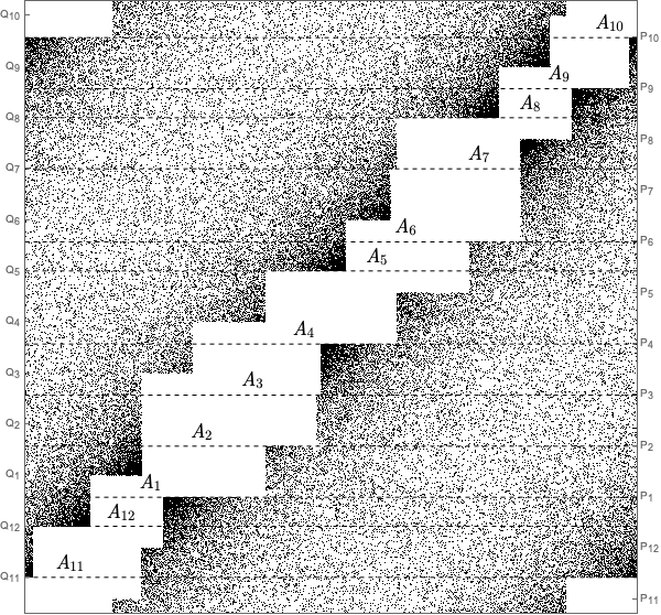
Figure 3. The domain $\Omega_{\,\overline{\!A\!}\,}$ for the extremal parameters in (9).

This section describes in detail the process by which the domain $\Omega_{\,\overline{\!A\!}\,}$ of $F_{\,\overline{\!A\!}\,}$ was realized, culminating with an explicit description (Equation 14) of $\Omega_{A}$ in 8.

From comparisons of numerical attractors for $F_{\,\overline{\!A\!}\,}$ with different extremal parameters, we conjectured that the corner points of $\Omega_{\,\overline{\!A\!}\,}$ for extremal ${\,\overline{\!A\!}\,}$ should be of the form $(\,\cdot\,,Q_{i})$ for lower corners and $(\,\cdot\,,P_{i})$ for upper corners. Recall the definition of $\sigma$ from (2), and define

$$\tau(i)=i+(4g-2)\quad\bmod 8g-4.$$ (7)

Careful analysis shows that if a set

$$\Lambda=\bigcup_{i=1}^{8g-4}[x^{\prime}_{i},x_{i-2}]\times[P_{i},Q_{i}]\cup[x^{\prime}_{i},x_{i-1}]\times[Q_{i},P_{i+1}]$$

were to satisfy $F_{\,\overline{\!A\!}\,}(\Lambda)=\Lambda$ for extremal ${\,\overline{\!A\!}\,}$, this would imply that

$$\left\{\begin{array}[]{ll}x_{\sigma(i)}=T_{i}x_{i-2}&\text{if }A_{i}=P_{i}\\ x^{\prime}_{\tau\sigma(i)}=T_{i-1}x^{\prime}_{i}&\text{if }A_{i}=Q_{i}.\end{array}\right.$$

Setting $x^{\prime}_{i}=T_{\sigma(i+1)}T_{\tau(i)}x_{\tau(i)}$, these relations can be stated in terms of $\{x_{i}\}$ only as

$$\left\{\begin{array}[]{ll}x_{\sigma(i)}=T_{i}x_{i-2}&\text{if }A_{i}=P_{i}\\ x_{\sigma(i)}=T_{\tau(i)+1}x_{\tau(i)}&\text{if }A_{i}=Q_{i}.\end{array}\right.$$

To that end, we prove 3 and ultimately 8.

Proposition 3.

For any extremal ${\,\overline{\!A\!}\,}$, there exist unique values $G_{1},\ldots,G_{8g-4}$ such that all of the following hold for all $1\leq i\leq 8g-4$:

• $G_{i}\in[P_{i},P_{i+1}]$,

• $G_{\sigma(i)}=T_{i}G_{i-2}$ if $A_{i}=P_{i}$,

• $G_{\sigma(i)}=T_{\tau(i)+1}G_{\tau(i)}$ if $A_{i}=Q_{i}$.

Before proving 3, it is instructive to work through one example of solving the system

$$G_{\sigma(i)}=\left\{\begin{array}[]{ll}T_{i}G_{i-2}&\text{if }A_{i}=P_{i}\\ T_{\tau(i)+1}G_{\tau(i)}&\text{if }A_{i}=Q_{i}\end{array}\right.$$ (8)

by hand. For this worked example, we consider the genus-$2$ parameter choice

$${\,\overline{\!A\!}\,}=\{P_{1},P_{2},P_{3},P_{4},Q_{5},P_{6},Q_{7},Q_{8},P_{9},P_{10},Q_{11},Q_{12}\}.$$ (9)

We want to find the values $G_{1},\ldots,G_{12}$ described by 3. Applying (8) with $i=1,\ldots,8g-4$ gives the following system of twelve equations:

1. $A_{1}=P_{1}\text{, we need }G_{7}=T_{1}G_{11}$.

2. $A_{2}=P_{2}\text{, we need }G_{12}=T_{2}G_{12}$.

3. $A_{3}=P_{3}\text{, we need }G_{5}=T_{3}G_{1}$.

4. $A_{4}=P_{4}\text{, we need }G_{10}=T_{4}G_{2}$.

5. $A_{5}=Q_{5}\text{, we need }G_{3}=T_{12}G_{11}$.

6. $A_{6}=P_{6}\text{, we need }G_{8}=T_{6}G_{4}$.

7. $A_{7}=Q_{7}\text{, we need }G_{1}=T_{2}G_{1}$.

8. $A_{8}=Q_{8}\text{, we need }G_{6}=T_{3}G_{2}$.

9. $A_{9}=P_{9}\text{, we need }G_{11}=T_{9}G_{7}$.

10. $A_{10}=P_{10}\text{, we need }G_{4}=T_{10}G_{8}$.

11. $A_{11}=Q_{11}\text{, we need }G_{9}=T_{6}G_{5}$.

12. $A_{12}=Q_{12}\text{, we need }G_{2}=T_{7}G_{6}$.

Line 1 is not immediately useful since neither $G_{7}$ nor $G_{11}$ is known. Line 2 tells us that $G_{12}$ is a fixed point of $T_{2}$. The fixed points of $T_{2}$ are $P_{1}$ and $Q_{2}$, and since we require $G_{i}\in[P_{i},P_{i+1}]$, we must use $G_{12}=P_{1}$. Likewise, Line 7 gives us that $G_{1}=P_{1}$ as well. Knowing that $G_{1}=P_{1}$, we can use Line 3 to get $G_{5}=T_{3}P_{1}$ and then Line 11 to get $G_{9}=T_{6}G_{5}=T_{6}T_{3}P_{1}$.

Combing Line 9 with Line 1 tells us that $G_{7}=T_{1}(T_{9}G_{7})$, and so $G_{7}$ is a fixed point of $T_{1}T_{9}$, whose fixed points are $P_{8}$ and $Q_{9}$, of which only $G_{7}=P_{8}$ fulfills the requirement $G_{i}\in[P_{i},P_{i+1}]$. Likewise $P_{12}$ is the only valid choice for $G_{11}$ from the two fixed points $P_{12}$ and $Q_{1}$ of $T_{9}T_{1}$. Knowing that $G_{11}=P_{12}$, Line 5 gives us $G_{3}=T_{12}G_{11}=T_{12}P_{12}=Q_{3}$.

The remaining $G_{i}$ values are determined by the same means. Figure 4 shows the system of twelve equations above as a graph, where the $G_{i}$ are vertices and each equation from the system is an edge. Vertices with a loop are fixed points of some $T_{k}$, and pairs of vertices in a two-cycle are fixed points of some $T_{\sigma(k)}T_{k+2}$. All other vertices connect through a single path (a “chain”) to either a fixed point of some $T_{k}$ or a fixed point of some $T_{\sigma(k)}T_{k+2}$.

Figure 4. The graph representing the system of equations (8) for the example parameters ${\,\overline{\!A\!}\,}$ in (9).

After resolving all loops, two-cycles, and chains in Figure 4, we get that the values $G_{i}$ from 3 for the specific example ${\,\overline{\!A\!}\,}$ in (9) are

$$G_{1} =P_{1} G_{4} =P_{5} G_{7} =P_{8} G_{10} =T_{4}P_{2}$$

$$G_{2} =P_{2} G_{5} =T_{3}P_{1} G_{8} =P_{9} G_{11} =P_{12}$$ (10)

$$G_{3} =Q_{3} G_{6} =P_{6} G_{9} =T_{6}T_{3}P_{1} G_{12} =P_{1}.$$

The proof of 3 presented in the remainder of this section shows that the graphs for any extremal ${\,\overline{\!A\!}\,}$ in any genus always a structure similar to the graph in Figure 4: there are loops and two-cycles that lead directly to values for certain $G_{i}$, and there are chains connecting unambiguously to a cycle, which determine the remaining $G_{i}$. The “types” in 4 provide a rigorous way to describe whether a particular $G_{i}$ is part of a cycle (Types 1 and 3) or part of a chain (Types 2 and 4), and 5 can be interpreted to mean that all chains must end (in either a loop or a two-cycle).

Definition 4.

We say that an index $i$ is

1. $A_{\sigma(i)}=P_{\sigma(i)}$ and $A_{i+2}=P_{i+2}$,

2. $A_{\sigma(i)}=P_{\sigma(i)}$ and $A_{i+2}=Q_{i+2}$,

3. $A_{\sigma(i)}=Q_{\sigma(i)}$ and $A_{\tau(i)}=Q_{\tau(i)}$,

4. $A_{\sigma(i)}=Q_{\sigma(i)}$ and $A_{\tau(i)}=P_{\tau(i)}$.

Note that each index is of exactly one type.

Lemma 5.

It cannot be that $i+4gn$ is Type 2 for all $n\geq 0$. It cannot be that $i-4gn$ is Type 4 for all $n\geq 0$.

Proof.

Assume that $i+4gn$ is Type 2 for all $n\geq 0$. That is, $A_{\sigma(i+4gn)}=P_{\sigma(i+4gn)}$ and $A_{(i+4gn)+2}=Q_{(i+4gn)+2}$ for all $n\geq 0$. Since ${\,\overline{\!P\!}\,}$ and $\,\overline{\!Q\!}\,$ are disjoint, this requires $\sigma(i+4gn)\not\equiv i+4gn+2~{}({\rm mod}~{}{8g-4})$ for all $n\geq 0$. By direct calculation,

$$\sigma(j)\equiv j+2\quad\iff\quad j\in\{2g-1,4g-2,6g-3,8g-4\}.$$

Since we are working mod $8g-4$, we can say that $\sigma(j)\equiv j+2$ whenever $j$ is any integer multiple of $2g-1$. Thus $i+4gn$ is not a multiple of $2g-1$ for any $n$.

If $i$ is even, let $n=K(2g-1)-\tfrac{i}{2}$ with $K$ large enough that $n>0$. Then

$$i+4gn =i+4g\big{(}2Kg-K-\tfrac{i}{2}\big{)}$$

$$=i+8Kg^{2}-4Kg-2gi$$

$$=(2g-1)(4Kg-i).$$

If $i$ is odd, let $n=K(2g-1)+(g-1)-\tfrac{i-1}{2}$ with $K$ large enough that $n>0$. Then

$$i+4gn =i+4g\big{(}2Kg-K+g-1-\tfrac{i-1}{2}\big{)}$$

$$=i+8Kg^{2}-4Kg+4g^{2}-2g-2gi$$

$$=(2g-1)(4Kg+2g-i).$$

In either case, there exists $n>0$ such that $i+4gn$ is a multiple of $2g-1$. As shown above, the assumption that $i+4gn$ is Type 2 for all $n\geq 0$ implies that $i+4gn$ is not a multiple of $2g-1$ for any $n$. This contradiction shows that $i+4gn$ cannot be Type 2 for all $n\geq 0$.

Similar arguments give a contradiction if $i-4gn$ is Type 4 for all $n\geq 0$. ∎

Lemma 6.

If $x\in[P_{j},P_{j+1}]$ then $T_{\tau\sigma(j)+2}T_{j+1}x\in[P_{\tau(j)-2},P_{\tau(j)-1}]$.

Proof.

Firstly,

$$T_{j+1}[P_{j},P_{j+1}]=[T_{j+1}P_{j},T_{j+1}P_{j+1}]=[P_{\tau\sigma(j)},Q_{\tau\sigma(j)}].$$

Setting $k=\tau\sigma(j)$, we now want to show that $T_{k+2}[P_{k},Q_{k}]\subset[P_{\sigma(k)-2},P_{\sigma(k)-1}]$. For any $k$, we have “$[P_{k},Q_{k}]\subset[Q_{k+3},P_{k+1}]$” in the sense that moving counter-clockwise around the circle one has $Q_{k+3},P_{k},Q_{k},P_{k+1}$ in that order. Applying $T_{k+2}$, which is monotonically “increasing” (counter-clockwise) on ${\mathbb{S}}$, we get

$$T_{k+2}[P_{k},Q_{k}]\subset[T_{k+2}Q_{k+3},T_{k+2}P_{k+1}]=[P_{\sigma(k)-2},P_{\sigma(k)-1}]$$

as desired. ∎

Proof of 3.

We will construct the solution to the system (8), that is,

$$G_{\sigma(i)}=\left\{\begin{array}[]{ll}T_{i}G_{i-2}&\text{if }A_{i}=P_{i}\\ T_{\tau(i)+1}G_{\tau(i)}&\text{if }A_{i}=Q_{i},\end{array}\right.$$

with $G_{i}\in[P_{i},P_{i+1}]$.

If $i$ is Type 1, then (8) tells us that

$$T_{\sigma(i)}G_{\sigma(i)-2}=G_{i}$$

because $A_{\sigma(i)}=P_{\sigma(i)}$, and because $A_{i+2}=P_{i+2}$ we have

$$T_{i+2}G_{i}=G_{\sigma(i)-2}.$$

Together, these imply that $G_{i}$ is a fixed point of $T_{\sigma(i)}T_{i+2}$. The fixed points of that map are $P_{i+1}$ and $Q_{i+2}$, and since we require $G_{i}\in[P_{i},P_{i+1}]$ it must be that $G_{i}=P_{i+1}$.

If $i$ is Type 3, then

$$T_{\tau\sigma(i)+1}G_{\tau\sigma(i)} =G_{i}$$

$$T_{i+1}G_{i} =G_{\tau\sigma(i)},$$

and so $G_{i}$ must be the fixed point $P_{i}$ of $T_{\tau\sigma(i)+1}T_{i+1}$.

If $i$ is Type 2, the condition $A_{\sigma(i)}=P_{\sigma(i)}$ implies

$$G_{i}=T_{\sigma(i)}G_{\sigma(i)-2},$$

and the condition $A_{i+2}=Q_{i+2}$ implies

$$G_{\sigma(i+2)} =T_{\tau(i+2)+1}G_{\tau(i+2)}$$

$$G_{\sigma(i)-2} =T_{\tau(i)+3}G_{\tau(i)+2}.$$

Using that $\tau(i)=i+4g-2$, we have

$$i\text{ is Type~{}\ref{type-PQ}}\quad\implies\quad G_{i}=T_{\sigma(i)}T_{\tau(i)+3}G_{i+4g}.$$ (11)

Consider the possible types of $i+4g$.

• If $i+4g$ is Type 1, then $G_{i+4g}=P_{i+4g+1}$, and by 6 we
  get $G_{i}\in[P_{i},P_{i+1}]$.

• If $i+4g$ is Type 3, then $G_{i+4g}=P_{i+4g}$, and by 6 we
  get $G_{i}\in[P_{i},P_{i+1}]$.

• If $i+4g$ is Type 4, then $A_{\tau(i+4g)}=A_{i+2}=P_{i+2}$, which contradicts $i$ being Type 2. So this cannot occur.

• If $i+4g$ is Type 2, the condition $A_{\sigma(i+4g)}=A_{\tau\sigma(i)-2}=P_{\tau\sigma(i)-2}$ gives

  $$G_{i+4g}=T_{\tau\sigma(i)-2}G_{\tau\sigma(i)-4}$$

  and the condition $A_{\tau(i)+4}=Q_{\tau(i)+4}$ gives

  $$G_{\sigma\tau(i)-4}=T_{i+5}G_{i+4}=T_{i+5}G_{i+8g}.$$

  Combining these with (11), we get

  $$G_{i}=T_{\sigma(i)}T_{\tau(i)+3}T_{\tau\sigma(i)-2}T_{i+5}(G_{i+8g}).$$ (12)

Notice that (11) gives $G_{i}$ in terms of $G_{i+4g}$, and now assuming $i+4g$ is Type 2 as well we have $G_{i}$ in terms of $G_{i+8g}$ from (12). Inductively, we continue to get expressions for $G_{i}$ in terms of $G_{i+4gn}$ so long as $G_{i+4g(n-1)}$ is Type 2. As with the third bullet above, any $i+4gn$ being Type 4 will cause an immediate contradiction, and by 5 we cannot have $i+4gn$ be Type 2 for all $n\geq 0$. Thus for some $n$ we must have $i+4gn$ of Type 1 or 3, at which point $G_{i+4gn}$ will be $P_{i+4gn+1}$ or $P_{i+4gn}$, respectively, and inductively this leads to a value for $G_{i}$ that by 6 will be in $[P_{i},P_{i+1}]$.

The case where $i$ is Type 4 is handled similarly to Type 2: we cannot have $i,i-4g,i-8g,i-12g$, etc., all be Type 4, none of them can be Type 2 without contradiction, and once we have $i-4gn$ being Type 1 or Type 3 we inductively get a unique value for $G_{i-4gk}$ in $[P_{i-4gk},P_{i-4gk+1}]$ for $k=n,n-1,\ldots,0$. ∎

Lemma 7.

Let $G_{1},G_{2},\ldots,G_{8g-4}$ be from 3, and denote

$$H_{i}:=U_{i}G_{\tau(i)-1}\qquad\text{and}\qquad D_{i}:=T_{\tau\sigma(i)+1}G_{\tau\sigma(i)},$$ (13)

where

$$U_{i}:=T_{\sigma(i-1)}T_{\tau(i)}=T_{\sigma(i)}T_{\tau(i)-1}.$$

Then the following hold:

1. $D_{i}=T_{\sigma(i)}H_{\sigma(i)+1}$,

2. $D_{i}\in[P_{i},Q_{i}]$,

3. $H_{i}\in[Q_{i},Q_{i+1}]$.

Proof.

The first item follows directly from the definitions of $H_{k}$, $U_{k}$, and $D_{i}$:

$$T_{\sigma(i)}H_{\sigma(i)+1} =T_{\sigma(i)}U_{\sigma(i)+1}G_{\tau(\sigma(i)+1)-1}=T_{\sigma(i)}T_{i}T_{\tau\sigma(i)+1}G_{\tau\sigma(i)}$$

$$=T_{\tau\sigma(i)+1}G_{\tau\sigma(i)}=D_{i}.$$

The latter items follow from simple calculations and the fact that $G_{k}\in[P_{k},P_{k+1}]$ for all $k$:

$$D_{i} \in T_{\tau\sigma(i)+1}[P_{\tau\sigma(i)},P_{\tau\sigma(i)+1}]=[P_{i},Q_{i}],$$

$$H_{i} \in U_{i}[P_{\tau(i)-1},P_{\tau(i)}]=[T_{\sigma(i)}T_{\tau(i)-1}P_{\tau(i)-1},T_{\sigma(i)}T_{\tau(i)-1}P_{\tau(i)}]$$

$$\qquad\qquad=[T_{\sigma(i)}Q_{\sigma(i)+2},T_{\sigma(i)}P_{\sigma(i)}]=[Q_{i},Q_{i+1}].\qed$$

We are now ready to prove one of the main results of this paper:

Theorem 8.

For any extremal parameter choice ${\,\overline{\!A\!}\,}$, the set

$$\Omega_{\,\overline{\!A\!}\,}:=\bigcup_{i=1}^{8g-4}\;[H_{i+1},G_{i-2}]\!\times\![P_{i},Q_{i}]\;\cup\;[H_{i+1},G_{i-1}]\!\times\![Q_{i},P_{i+1}]$$ (14)

is a bijectivity domain for $F_{\,\overline{\!A\!}\,}$, where $\{G_{i}\}$ are from 3 and $\{H_{i}\}$ are from Equation 13.

Proof.

Label the horizontal strips of $\Omega_{\,\overline{\!A\!}\,}$ as

$$\begin{split}R_{i}^{\prime\prime}&:=[H_{i+1},G_{i-2}]\times[P_{i},Q_{i}]\\ R_{i}^{\prime}&:=[H_{i+1},G_{i-1}]\times[Q_{i},P_{i+1}],\end{split}$$ (15)

so $\Omega_{\,\overline{\!A\!}\,}=\bigcup_{i=1}^{8g-4}(R_{i}^{\prime\prime}\cup R_{i}^{\prime})$. From 7(1), we have that $T_{i}H_{i+1}=D_{\sigma(i)}$, where $\{D_{i}\}$ are defined in (13), so we compute that

$$T_{i}R_{i}^{\prime} =[T_{i}H_{i+1},T_{i}G_{i-1}]\times[T_{i}Q_{i},T_{i}P_{i+1}]$$

$$=[D_{\sigma(i)},D_{\sigma(i)+1}]\times[Q_{\sigma(i)+2},P_{\sigma(i)-1}].$$

We also compute

$$T_{i}R_{i}^{\prime\prime} =[T_{i}H_{i+1},T_{i}G_{i-2}]\times[T_{i}P_{i},T_{i}Q_{i}]$$

$$=[D_{\sigma(i)},T_{i}G_{i-2}]\times[Q_{\sigma(i)+1},Q_{\sigma(i)+2}]$$

$$=[D_{\sigma(i)},G_{\sigma(i)}]\times[Q_{\sigma(i)+1},Q_{\sigma(i)+2}]\qquad\text{if }A_{i}=P_{i}$$

and

$$T_{i-1}R_{i}^{\prime\prime} =[T_{i-1}H_{i+1},T_{i-1}G_{i-2}]\times[T_{i-1}P_{i},T_{i-1}Q_{i}]$$

$$=[T_{i-1}H_{i+1},D_{\tau\sigma(i)+2}]\times[P_{\tau\sigma(i)},P_{\tau\sigma(i)+1}]$$

$$=[H_{\tau\sigma(i)},D_{\tau\sigma(i)+2}]\times[P_{\tau\sigma(i)},P_{\tau\sigma(i)+1}]\qquad\text{if }A_{i}=Q_{i}.$$

The image of $\Omega_{\,\overline{\!A\!}\,}$ under $F_{\,\overline{\!A\!}\,}$ is therefore

$$F_{\,\overline{\!A\!}\,}(\Omega_{\,\overline{\!A\!}\,}) =\bigcup_{i=1}^{8g-4}T_{\ell}R_{i}^{\prime\prime}\cup T_{i}R^{\prime}_{i},\quad\text{where }\ell=\big{\{}\begin{smallmatrix}i\phantom{-1}&\text{if }A_{i}=P_{i}\\ i-1&\text{if }A_{i}=Q_{i}\end{smallmatrix}$$

$$=\bigcup_{i=1}^{8g-4}T_{i}R_{i}^{\prime}\;\;\cup\bigcup_{i:\>A_{i}=P_{i}}\!\!T_{i}R_{i}^{\prime\prime}\;\;\cup\bigcup_{i:\>A_{i}=Q_{i}}\!\!T_{i-1}R_{i}^{\prime\prime}$$

$$=\bigcup_{i=1}^{8g-4}[D_{\sigma(i)},D_{\sigma(i)+1}]\times[Q_{\sigma(i)+2},P_{\sigma(i)-1}]$$

$$\qquad\cup\bigcup_{i:\>A_{i}=P_{i}}\!\![D_{\sigma(i)},G_{\sigma(i)}]\times[Q_{\sigma(i)+1},Q_{\sigma(i)+2}]$$

$$\qquad\cup\bigcup_{i:\>A_{i}=Q_{i}}\!\![H_{\tau\sigma(i)},D_{\tau\sigma(i)+2}]\times[P_{\tau\sigma(i)},P_{\tau\sigma(i)+1}]$$

$$=\bigcup_{j=1}^{8g-4}[D_{j},D_{j+1}]\times[Q_{j+2},P_{j-1}]$$

$$\qquad\cup\bigcup_{i:\>A_{i}=P_{i}}[D_{j},G_{j}]\times[Q_{j+1},Q_{j+2}],\qquad j=\sigma(i)$$

$$\qquad\cup\bigcup_{i:\>A_{i}=Q_{i}}[H_{k},D_{k+2}]\times[P_{k},P_{k+1}],\qquad k=\tau\sigma(i).$$

Note that the images $T_{i}R_{i}^{\prime}$ are quite tall since $[Q_{j+2},P_{j-1}]$ contains more than half of ${\mathbb{S}}$. The images $T_{\ell}R_{i}^{\prime\prime}$ are not tall (regardless of whether $A_{i}$ is $P_{i}$ or $Q_{i}$).

Using the inclusions of 7, we have

$$\begin{split}F_{\,\overline{\!A\!}\,}(\Omega_{\,\overline{\!A\!}\,})&=\bigcup_{j=1}^{8g-4}\underbrace{[D_{j},D_{j+1}]}_{\subset\;[P_{j},Q_{j+1}]}\times[Q_{j+2},P_{j-1}]\\ &\qquad\cup\bigcup_{i:\>A_{i}=P_{i}}\underbrace{[D_{j},G_{j}]}_{\subset\;[P_{j},P_{j+1}]}\times[Q_{j+1},Q_{j+2}],\qquad j=\sigma(i)\\ &\qquad\cup\bigcup_{i:\>A_{i}=Q_{i}}\underbrace{[H_{k},D_{k+1}]}_{\subset\;[Q_{k},Q_{k+1}]}\times[P_{k-1},P_{k}],\qquad k=\tau\sigma(i)+1.\end{split}$$ (16)

The right-hand side of (16) has expressions for $3\times(8g-4)$ rectangles. Which of these intersect ${\mathbb{S}}\times[P_{m},Q_{m}]$ for a fixed $m$? Looking at the $y$-projection of these rectangles, we see that

• $[Q_{j+2},P_{j-1})$ intersects $[P_{m},Q_{m}]$ if and only if $j\notin\{m\!-\!2,\,m\!-\!1,\,m,\,m\!+\!1\}$;

• $(Q_{j+1},Q_{j+2}]$ intersects $[P_{m},Q_{m}]$ exactly when $j=m-2$;

• $[P_{k-1},P_{k})$ intersects $[P_{m},Q_{m}]$ exactly when $k=m+1$.

This gives us a smaller collection of rectangles whose union is contained in $F_{\,\overline{\!A\!}\,}(\Omega_{\,\overline{\!A\!}\,})$ and entirely contains the intersection of $F_{\,\overline{\!A\!}\,}(\Omega_{\,\overline{\!A\!}\,})$ with ${\mathbb{S}}\times[P_{m},Q_{m}]$.

$$F_{\,\overline{\!A\!}\,}(\Omega_{\,\overline{\!A\!}\,})\cap\big{(}{\mathbb{S}}\times[Q_{m},P_{m+1}]\big{)}\subset\left(\begin{array}[]{l}[D_{m-2},G_{m-2}]\times[Q_{m-1},Q_{m}]\\ \cup\;[H_{m+1},D_{m+2}]\times[P_{m},P_{m+1}]\\ \displaystyle\cup\bigcup_{\begin{subarray}{c}j\neq m\!-\!2,j\neq m\!-\!1,\\ j\neq m,\,j\neq m\!+\!1\end{subarray}}[D_{j},D_{j+1}]\times[Q_{j+2},P_{j-1}]\end{array}\!\!\!\right)\subset F_{\,\overline{\!A\!}\,}(\Omega_{\,\overline{\!A\!}\,}).$$

The rectangles on the right-hand side above can each be vertically truncated to contain only their intersection with ${\mathbb{S}}\times[P_{m},Q_{m}]$, giving that

$$F_{\,\overline{\!A\!}\,}(\Omega_{\,\overline{\!A\!}\,})\cap\big{(}{\mathbb{S}}\times[Q_{m},P_{m+1}]\big{)}$$

$$=[D_{m-2},G_{m-2}]\times[P_{m},Q_{m}]\cup[H_{m+1},D_{m+2}]\times[P_{m},Q_{m}]$$

$$\qquad\cup\bigcup_{\begin{subarray}{c}j\neq m\!-\!2,j\neq m\!-\!1,\\ j\neq m,\,j\neq m\!+\!1\end{subarray}}[D_{j},D_{j+1}]\times[P_{m},Q_{m}]$$

$$=\left([D_{m-2},G_{m-2}]\cup[H_{m+1},D_{m+2}]\cup\bigcup_{\begin{subarray}{c}j\neq m\!-\!2,j\neq m\!-\!1,\\ j\neq m,\,j\neq m\!+\!1\end{subarray}}[D_{j},D_{j+1}]\right)\times[P_{m},Q_{m}]$$

$$=\left([H_{m+1},D_{m+2}]\cup\left(\begin{array}[]{l}[D_{m+2},D_{m+3}]\\ \cup[D_{m+3},D_{m+4}]\\ \cup\cdots\\ \cup[D_{m-3},D_{m-2}]\end{array}\right)\cup[D_{m-2},G_{m-2}]\right)\times[P_{m},Q_{m}]$$

$$=[H_{m+1},G_{m-2}]\times[P_{m},Q_{m}]$$

This is exactly $R_{m}^{\prime\prime}$. Similar arguments show that $F_{\,\overline{\!A\!}\,}(\Omega_{\,\overline{\!A\!}\,})\cap\big{(}{\mathbb{S}}\times[Q_{m},P_{m+1}]\big{)}$ is exactly $R_{m}^{\prime}$, and therefore $F_{\,\overline{\!A\!}\,}(\Omega_{\,\overline{\!A\!}\,})=\bigcup_{m=1}^{8g-4}(R_{m}^{\prime\prime}\cup R_{m}^{\prime})=\Omega_{\,\overline{\!A\!}\,}$. ∎

2.2. Conjugacy and cross-section

In [4, Section 5], a conjugacy between $F_{\mathrm{geo}}:\Omega_{\mathrm{geo}}\to\Omega_{\mathrm{geo}}$ and $F_{\,\overline{\!P\!}\,}:\Omega_{\,\overline{\!P\!}\,}\to\Omega_{\,\overline{\!P\!}\,}$ is provided, and in [1, Section 3] similar techniques are used to construct a conjugacy between $F_{\mathrm{geo}}:\Omega_{\mathrm{geo}}\to\Omega_{\mathrm{geo}}$ and $F_{\,\overline{\!A\!}\,}:\Omega_{\,\overline{\!A\!}\,}\to\Omega_{\,\overline{\!A\!}\,}$ in the case where ${\,\overline{\!A\!}\,}$ satisfies the short cycle property. In this section, that result is extended to all extremal parameters.

First, we define bulges and corners:

Definition 9.

For $1\leq i\leq 8g-4$, the lower bulge ${\mathcal{B}}_{i}$, the upper bulge ${\mathcal{B}}^{i}$, the lower corner ${\mathcal{C}}_{i}$, and the upper corner ${\mathcal{C}}^{i}$ are given by

$$\begin{split}{\mathcal{B}}_{i}&=(\Omega_{\mathrm{geo}}\setminus\Omega_{\,\overline{\!A\!}\,})\;\cap\;\big{(}[Q_{i+1},Q_{i+2}]\!\times\![P_{i},P_{i+1}]\big{)}\\ {\mathcal{B}}^{i}&=(\Omega_{\mathrm{geo}}\setminus\Omega_{\,\overline{\!A\!}\,})\;\cap\;\big{(}[P_{i-1},P_{i}]\!\times\![Q_{i},Q_{i+1}]\big{)}\\ {\mathcal{C}}_{i}&=(\Omega_{\,\overline{\!A\!}\,}\setminus\Omega_{\mathrm{geo}})\;\cap\;\big{(}[Q_{i+1},Q_{i+2}]\!\times\![P_{i},P_{i+1}]\big{)}\\ {\mathcal{C}}^{i}&=(\Omega_{\,\overline{\!A\!}\,}\setminus\Omega_{\mathrm{geo}})\;\cap\;\big{(}[P_{i-1},P_{i}]\!\times\![Q_{i},Q_{i+1}]\big{)}.\end{split}$$

Note that for a given extremal ${\,\overline{\!A\!}\,}$, some bulges or corners may have empty interiors.

Figure 5. Comparison of bulges and corners for short cycle and extremal parameters. Bulges ${\mathcal{B}}^{i}$ in blue and ${\mathcal{B}}_{i}$ in gold; corners ${\mathcal{C}}^{i}$ in red and ${\mathcal{C}}_{i}$ in green.

Proposition 10.

The map $\Phi$ with domain $\Omega_{\mathrm{geo}}$ given by

$$\Phi=\left\{\begin{array}[]{ll}\mathrm{Id}&\text{on }\Omega_{\mathrm{geo}}\cap\Omega_{\,\overline{\!A\!}\,}\\ U_{\tau(i)+1}&\text{on }{\mathcal{B}}_{i}\\ U_{\tau(i)}&\text{on }{\mathcal{B}}^{i}\end{array}\right.$$ (17)

is a bijection from $\Omega_{\mathrm{geo}}$ to $\Omega_{\,\overline{\!A\!}\,}$. Specifically, $\Phi({\mathcal{B}}_{i})={\mathcal{C}}^{\tau(i)+1}$ and $\Phi({\mathcal{B}}^{i})={\mathcal{C}}_{\tau(i)-1}$.

Proof.

All the sets ${\mathcal{B}}_{i},{\mathcal{B}}^{i},{\mathcal{C}}_{i},{\mathcal{C}}^{i}$ are bounded by one horizontal line segment, one vertical line segment, and one curved segment that is part of $\partial\Omega_{\mathrm{geo}}$. Since each $U_{j}$ is a Möbius transformation, we need only to show that these boundaries are mapped accordingly. The boundaries of ${\mathcal{B}}_{i}$ are the horizontal segment $[Q_{i+1},H_{i+1}]\times\{P_{i}\}$, part of the vertical segment $\{H_{i+1}\}\times[P_{i},P_{i+1}]$, and part of the segment of $\partial\Omega_{\mathrm{geo}}$ connecting $(Q_{i+1},P_{i})$ to $(Q_{i+2},P_{i+1})$. By definition, $\Phi({\mathcal{B}}_{i})=U_{\tau(i)+1}({\mathcal{B}}_{i})$. As calculated in the proof of [1, Proposition 3.4],

$$U_{\tau(i)+1}P_{i} =Q_{\tau(i)+1}, U_{\tau(i)+1}Q_{i+1} =P_{\tau(i)},$$

$$U_{\tau(i)+1}P_{i+1} =Q_{\tau(i)+2}, U_{\tau(i)+1}Q_{i+2} =P_{\tau(i)-1}.$$

Additionally, since $H_{j}=U_{j}G_{\tau(j+1)}$ by definition and $U_{\tau(i)+1}=U_{i+1}^{-1}$, we have

$$U_{\tau(i)+1}H_{i+1}=U_{\tau(i)+1}U_{i+1}G_{\tau(i)}=G_{\tau(i)}.$$

Therefore

$$U_{\tau(i)+1}\big{(}[Q_{i+1},H_{i+1}]\times\{P_{i}\}\big{)} =[P_{\tau(i)},G_{\tau(i)}]\times\{Q_{\tau(i)+1}\},$$

$$U_{\tau(i)+1}\big{(}\{H_{i+1}\}\times[P_{i},P_{i+1}]\big{)} =\{G_{\tau(i)}\}\times[Q_{\tau(i)+1},Q_{\tau(i)+2}],$$

$$U_{\tau(i)+1}(Q_{i+1},P_{i}) =(P_{\tau(i)},Q_{\tau(i)+1}),$$

$$U_{\tau(i)+1}(Q_{i+2},P_{i+1}) =(P_{\tau(i)-1},Q_{\tau(i)+2}).$$

The corner ${\mathcal{C}}^{\tau(i)+1}$ is exactly the set bounded by the horizontal segment $[P_{\tau(i)},G_{\tau(i)}]\times\{Q_{\tau(i)+1}\}$, part of the vertical segment $\{G_{\tau(i)}\}\times[Q_{\tau(i)+1},Q_{\tau(i)+2}]$, and part of segment of $\partial\Omega_{\mathrm{geo}}$ connecting $(P_{\tau(i)},Q_{\tau(i)+1})$ to $(P_{\tau(i)+1},Q_{\tau(i)+2})$. Thus $U_{\tau(i)+1}({\mathcal{B}}_{i})={\mathcal{C}}^{\tau(i)+1}$. A similar argument shows $U_{\tau(i)}({\mathcal{B}}^{i})={\mathcal{C}}_{\tau(i)-1}$. Taking $\Phi(\Omega_{\mathrm{geo}}\cap\Omega_{\,\overline{\!A\!}\,})=\Omega_{\mathrm{geo}}\cap\Omega_{\,\overline{\!A\!}\,}$ (since $\Phi=\mathrm{Id}$ on that set) together with $\Phi({\mathcal{B}}_{i})={\mathcal{C}}^{\tau(i)+1}$ and $\Phi({\mathcal{B}}^{i})={\mathcal{C}}_{\tau(i)-1}$, we have that $\Phi(\Omega_{\mathrm{geo}})=\Omega_{\,\overline{\!A\!}\,}$. ∎

Definition 11.

Let $u,w\in{\mathbb{S}}=\partial{\mathbb{D}}$, $u\neq w$. An oriented geodesic in ${\mathbb{D}}$ from $u$ to $w$ is called ${\,\overline{\!A\!}\,}$-reduced if $(u,w)\in\Omega_{\,\overline{\!A\!}\,}$.

10 implies the following important facts:

Corollary 12.

Let ${\,\overline{\!A\!}\,}$ be extremal, and let $\gamma=uw$ be a geodesic on ${\mathbb{D}}$.

1. If $\gamma$ intersects ${\mathcal{F}}$, then either $\gamma$ is ${\,\overline{\!A\!}\,}$-reduced or $U_{j}\gamma$ is ${\,\overline{\!A\!}\,}$-reduced, where $j=\tau(i)$ if $(u,w)\in{\mathcal{B}}^{i}$ and $j=\tau(i)+1$ if $(u,w)\in{\mathcal{B}}_{i}$.

2. If $\gamma$ is ${\,\overline{\!A\!}\,}$-reduced, then either $\gamma$ intersects ${\mathcal{F}}$ or $\gamma$ intersects $U_{j}({\mathcal{F}})$, where $j=i$ if $(u,w)\in{\mathcal{C}}^{i}$ and $j=i+1$ if $(u,w)\in{\mathcal{C}}_{i}$.

Using 12, we can define the arithmetic cross-section.

Definition 13.

For $(u,w)\in\Omega_{\,\overline{\!A\!}\,}$, denote by $\varphi(u,w)$ the point $(z^{\prime},\zeta^{\prime})$ in $S{\mathbb{D}}$ where either $\gamma$ enters ${\mathcal{F}}$, or, if $\gamma$ does not intersect ${\mathcal{F}}$, the first entrance point of $\gamma$ to $U_{j}{\mathcal{F}}$, where $j$ is as in 12(2). We define the arithmetic cross-section $C_{\,\overline{\!A\!}\,}=\pi\circ\varphi(\Omega_{\,\overline{\!A\!}\,})$, where $\pi$ is the canonical projection from $S{\mathbb{D}}$ to $SM$.

Remark 14.

The geometric cross-section $C_{\mathrm{geo}}$ initially described in Section 1 can be presented in an analogous way to 13. For $(u,w)\in\Omega_{\mathrm{geo}}$, denote by $\psi(u,w)$ the point $(z,\zeta)\in S{\mathbb{D}}$ such that $\gamma$ enters ${\mathcal{F}}$ at $z$. Then $C_{\mathrm{geo}}$ is exactly $\pi\circ\psi(\Omega_{\mathrm{geo}})$.

Proposition 15.

The map $\Phi:\Omega_{\mathrm{geo}}\to\Omega_{\,\overline{\!A\!}\,}$ in (17) is a conjugacy between $F_{\mathrm{geo}}$ and $F_{\,\overline{\!A\!}\,}$, that is, $\Phi\circ F_{\mathrm{geo}}=F_{\,\overline{\!A\!}\,}\circ\Phi$.

Corollary 16.

For each extremal parameter choice ${\,\overline{\!A\!}\,}$, the arithmetic cross-section $C_{\,\overline{\!A\!}\,}$ and the geometric cross-section $C_{\mathrm{geo}}$ are equal. Moreover, the first return of a tangent vector in $C_{\mathrm{geo}}$ to $C_{\mathrm{geo}}$ is also its first return to $C_{\,\overline{\!A\!}\,}$.

The proof of 15 is extremely similar to the proofs of [4, Theorem 5.2] and [1, Theorem 3.10], so we omit it here.

Proof of 16.

We use the maps $\pi\circ\varphi:\Omega_{\,\overline{\!A\!}\,}\to C_{\,\overline{\!A\!}\,}$ and $\pi\circ\psi:\Omega_{\mathrm{geo}}\to{\mathbb{C}}_{\mathrm{geo}}$ from 13 and Remark 14, respectively. Since $\pi\circ\varphi$, $\pi\circ\psi$, and $\Phi$ are bijections and $\Phi$ acts by elements of $\Gamma$, the diagram

(18)

commutes. Indeed, let $\gamma=uw$ with $(u,w)\in\Omega_{\mathrm{geo}}$. If $\gamma$ is ${\,\overline{\!A\!}\,}$-reduced, then $\Phi=\mathrm{Id}$, $\varphi=\psi$, and the diagram commutes trivially. If not, then the geodesic $U_{j}\gamma$ is ${\,\overline{\!A\!}\,}$-reduced for the index $1\leq j\leq 8g-4$ determined in 12(1); in this case $\Phi=U_{j}$ and thus $\varphi\circ\Phi=\psi$, so we have $\pi\circ\varphi\circ\Phi=\pi\circ\psi$ as well.

Combining the diagram (18) with 15, we obtain the diagram

The composition of the maps in the upper and lower rows are the first return maps to $C_{\mathrm{geo}}$ and $C_{\,\overline{\!A\!}\,}$, respectively, so the result follows from commutativity of the diagram. ∎

Remark 17.

The set $\Omega_{\,\overline{\!A\!}\,}$ is also thought to be the global attractor of $F_{\,\overline{\!A\!}\,}$ as a map on ${\mathbb{S}}\times{\mathbb{S}}\setminus\Delta$, $\Delta=\left\{\,(x,x):x\in{\mathbb{S}}\,\right\}$, meaning that $\bigcap_{n=0}^{\infty}F_{\,\overline{\!A\!}\,}^{n}({\mathbb{S}}\times{\mathbb{S}}\setminus\Delta)=\Omega_{\,\overline{\!A\!}\,}$, but a proof of this is not currently known. While this attractor property is a crucial part of Zagier’s “Reduction Theory” (see [10, 12]), it not a part of Adler and Flatto’s work on $\Gamma\backslash{\mathbb{D}}$.

2.3. Symbolic coding of geodesics

Coding of geodesics for parameters ${\,\overline{\!A\!}\,}$ such that $\Omega_{\,\overline{\!A\!}\,}$ possesses a finite rectangular structure is described in [1, Section 5]. The proofs in that section do not depend explicitly on the short cycle property (indeed, it is even stated that they apply to ${\,\overline{\!A\!}\,}=\,\overline{\!P\!}\,$) but rather on [1, Corollaries 3.6 and 3.8], which 12 here states for extremal parameters. Thus the results of [1, Section 5] do apply to all extremal parameters.

Definition 18.

Let $\gamma=uw$ be a geodesic on ${\mathbb{D}}$ with $(u,w)\in\Omega_{\,\overline{\!A\!}\,}$, and denote $(u_{k},w_{k})=F_{\,\overline{\!A\!}\,}^{k}(u,w)$ for all $k\in{\mathbb{Z}}$. The arithmetic code of $\gamma$ is the two-sided sequence

$$[\gamma]_{\,\overline{\!A\!}\,}=(\ldots,n_{-2},n_{-1},n_{0},n_{1},n_{2},\ldots)$$ (19)

where $n_{k}=\sigma(i)$ for the index $i$ such that $w_{k}\in[A_{i},A_{i+1})$.

A sequence $\overline{x}\in\{1,2,\ldots,8g-4\}^{\mathbb{Z}}$ is called admissible if it can be obtained by the coding procedure above for some geodesic $uw$ with $(u,w)\in\Omega_{\,\overline{\!A\!}\,}$. Given an admissible sequence $\overline{x}$, we can associate to it a vector $\operatorname{Cod}(\overline{x})\in SM$ as described in [1, Section 5]. The map $\operatorname{Cod}$ is finite-to-one and is uniformly continuous on the set of admissible coding sequences [1, Proposition 5.3], and thus we can extend it to the closure $X_{\,\overline{\!A\!}\,}$ of the set of all admissible sequences. In this way we associate to each ${\,\overline{\!A\!}\,}$ a symbolic system $(X_{\,\overline{\!A\!}\,},\sigma)$, and the geodesic flow becomes a special flow over $(X_{{\,\overline{\!A\!}\,}},\sigma)$ with the ceiling function $g_{{\,\overline{\!A\!}\,}}(\overline{x})$ on $X_{{\,\overline{\!A\!}\,}}$ being the time of the first return to the cross-section $C_{\,\overline{\!A\!}\,}$ of the geodesic associated to $\overline{x}$.

Proposition 19.

For any extremal parameters ${\,\overline{\!A\!}\,}$, the collection of all sets $[P_{i},Q_{i}]$ and $[Q_{i},P_{i+1}]$ forms a Markov partition for $f_{\,\overline{\!A\!}\,}$.

Proof.

The boundaries of Markov partition elements are measure zero, so we look at $16g-8$ total open intervals, which we denote here by $I_{2i-1}=(P_{i},Q_{i})$ and $I_{2i}=(Q_{i},P_{i+1})$. Using [12, Proposition 2.2], we have

$$\begin{split}f_{\,\overline{\!A\!}\,}(I_{2i})&=T_{i}(Q_{i},P_{i+1})=(P_{\sigma(i)+1},P_{\sigma(i)-2})\\ &=I_{2\sigma(i)+1}\cup I_{2\sigma(i)+1}\cup I_{2\sigma(i)+3}\cup\cdots\cup I_{2\sigma(i)-3}\cup I_{2\sigma(i)-2}.\end{split}$$

If $A_{i}=P_{i}$, then

$$f_{\,\overline{\!A\!}\,}(I_{2i-1})=T_{i}(P_{i},Q_{i})=(Q_{\sigma(i)+1},Q_{\sigma(i)+2})=I_{2\sigma(i)+2}\cup I_{2\sigma(i)+3},$$

and if $A_{i}=Q_{i}$ then

$$f_{\,\overline{\!A\!}\,}(I_{2i-1})=T_{i-1}(P_{i},Q_{i})=(P_{\tau\sigma(i)},P_{\tau\sigma(i)+1})=I_{2\tau\sigma(i)-1}\cup I_{2\tau\sigma(i)}.$$

Thus, for every $1\leq k\leq 16g-8$, we have that $f_{\,\overline{\!A\!}\,}(I_{k})$ is a union of some sets $I_{j}$. ∎

As described in [4, Appendix C], sofic systems are obtained from Markov ones by amalgamation of the alphabet, and, conversely, Markov is obtained from sofic by refinement of the alphabet. Thus, combining each pair $I_{2k-1}$ and $I_{2k}$ into a single interval $[P_{k},P_{k+1})$ gives the following:

Corollary 20.

For any extremal parameters ${\,\overline{\!A\!}\,}$, the shift on $X_{\,\overline{\!A\!}\,}$ is sofic with respect to the alphabet $\{1,2,\ldots,8g-4\}$.

3. Dual parameters

The “future” of an arithmetic code $[uw]_{\,\overline{\!A\!}\,}$, that is, the terms $n_{k}$ with $k\geq 0$, can be determined from $w$ alone, but the “past” ($k<0$) generally depends on both $u$ and $w$. For $(a,b)$-continued fractions, the existence of “dual codes” (see [11, Section 5]) for certain parameters allows the digits of the past to be determined from a single endpoint in those cases, and indeed a similar phenomenon can occur in the cocompact Fuchsian setting.

Definition 21.

Let ${\,\overline{\!A\!}\,}=\{A_{i}\}$ and ${\,\overline{\!D\!}\,}=\{D_{i}\}$ be two parameter choices for boundary maps from the same surface $M=\Gamma\backslash{\mathbb{D}}$ such that $F_{\,\overline{\!A\!}\,}$ and $F_{{\,\overline{\!D\!}\,}}$ have domains $\Omega_{\,\overline{\!A\!}\,}$ and $\Omega_{{\,\overline{\!D\!}\,}}$, respectively, with finite rectangular structure, and let $\phi(x,y)=(y,x)$. We say that ${\,\overline{\!D\!}\,}$ is dual to ${\,\overline{\!A\!}\,}$ if $\phi(\Omega_{\,\overline{\!A\!}\,})=\Omega_{\,\overline{\!D\!}\,}$ and $\phi(F_{\,\overline{\!A\!}\,}^{-1}(p))=F_{\,\overline{\!D\!}\,}(\phi(p))$ for all $p=(u,w)\in\Omega_{\,\overline{\!A\!}\,}$ with $u\notin{\,\overline{\!D\!}\,}$.

Theorem 22 ([1, Theorem 9.2]).

If ${\,\overline{\!D\!}\,}$ is dual to ${\,\overline{\!A\!}\,}$ and $(u,w)\in\Omega_{\,\overline{\!A\!}\,}$, then the arithmetic code $[\gamma]_{\,\overline{\!A\!}\,}$ of the geodesic $\gamma=uw$ satisfies

• for $k\geq 0$, $n_{k}$ is the value of $i$ for which $f_{\,\overline{\!A\!}\,}^{k}(w)\in[A_{\sigma(i)},A_{\sigma(i)+1})$, and

• for $k<0$, $n_{k}$ is the value of $i$ for which $f_{{\,\overline{\!D\!}\,}}^{-k+1}(u)\in[D_{i},D_{i+1})$.

Dual codes do not exist within the class of parameters with short cycles [1, Proposition 9.3]. Prior to 2018, the only known examples of dual parameters were $\,\overline{\!P\!}\,$ and $\,\overline{\!Q\!}\,$, both of which are extremal, and in fact a search for additional examples of duality was a primary motivation for studying the class of extremal parameters. 23 shows that every extremal ${\,\overline{\!A\!}\,}$ has a corresponding dual parameter set.

Theorem 23.

Given any extremal parameters ${\,\overline{\!A\!}\,}$, the parameter choice ${\,\overline{\!D\!}\,}=\{D_{1},$ …, $D_{8g-4}\}$ from 3 and Equation 13 is dual to ${\,\overline{\!A\!}\,}$.

Note that ${\,\overline{\!D\!}\,}$ is not necessarily extremal, nor will it satisfy the short cycle property. Since ${\,\overline{\!D\!}\,}$ may not satisfy the conditions of 8 or [12, Theorem 1.3], the domain for $F_{\,\overline{\!D\!}\,}$ must be described and proven independently.

Theorem 24.

Given any extremal parameters ${\,\overline{\!A\!}\,}$, let $\{G_{i}\}$, $\{H_{i}\}$, and $\{D_{i}\}$ be given by 3 and Equation 13. Then then set

$$\Omega_{\,\overline{\!D\!}\,}:=\bigcup_{i=1}^{8g-4}\raisebox{-5.0pt}{$\begin{array}[]{ll}[Q_{i+2},P_{i-1}]\!\times\![D_{i},D_{i+1}]\\ \quad\cup\;[P_{i-1},P_{i}]\!\times\![H_{i},D_{i+1}]\;\cup\;[Q_{i+1},Q_{i+2}]\!\times\![D_{i},G_{i}]\end{array}$}$$ (20)

is a bijectivity domain for the map $F_{\,\overline{\!D\!}\,}$.

Proof.

Define the following rectangles:

$$R_{i} :=[Q_{i+2},P_{i-1}]\times[D_{i},D_{i+1})$$

$$R_{i}^{u} :=[P_{i-1},P_{i}]\times[H_{i},D_{i+1})$$

$$R_{i}^{\ell} :=[Q_{i+1},Q_{i+2}]\times[D_{i},G_{i}].$$

These rectangles may have empty interior (see Cases II and IV below), but we include them in calculations for now.

Although initially $\Omega_{\,\overline{\!D\!}\,}$ was defined as $\bigcup_{i=1}^{8g-4}R_{i}\cup R_{i}^{u}\cup R_{i}^{\ell}$, it can equivalently be described via a decomposition into vertical strips as $\Omega_{\,\overline{\!D\!}\,}=\bigcup_{i=1}^{8g-4}V_{i}\cup V_{i}^{\prime}$, where

$$\begin{split}V_{i}&:=[P_{i},Q_{i}]\times[H_{i+1},G_{i-2})\\ V_{i}^{\prime}&:=[Q_{i},P_{i+1}]\times[H_{i+1},G_{i-1}).\end{split}$$ (21)

The map $F_{\,\overline{\!D\!}\,}$ acts on the rectangles $R_{i},R_{i}^{u},R_{i}^{\ell}$ by $T_{i}$. From 7(1), we have $T_{i}D_{i}=H_{\sigma(i)+1}$ for all $i$, and from the definition of $D_{i+1}$ we have $T_{i}D_{i+1}=G_{\sigma(i)-1}$ for all $i$. Setting $j=\sigma(i)$ for the remainder of this proof, we have

$$F_{\,\overline{\!D\!}\,}R_{i} =[T_{i}Q_{i+2},T_{i}P_{i-1}]\times[T_{i}D_{i},T_{i}D_{i+1})$$

$$=[Q_{j},P_{j+1}]\times[H_{j+1},G_{j-1})$$

$$=V_{j}^{\prime}.$$

We now consider the following four cases:

1. $A_{j}=P_{j}$.

2. $A_{j}=Q_{j}$.

3. $A_{j+1}=Q_{j+1}$.

4. $A_{j+1}=P_{j+1}$.

Note that Cases I and II are mutually exclusive, as are Cases III and IV.

Case I. When $A_{j}=P_{j}$, (8) gives

$$G_{i}=G_{\sigma(j)}=T_{j}G_{j-2},$$

and applying $T_{i}=T_{j}^{-1}$ to the left and right sides gives $T_{i}G_{i}=G_{j-2}$. From 7(1), we have $T_{i}D_{i}=H_{\sigma(i)+1}$ for all $i$. Thus

$$F_{\,\overline{\!D\!}\,}R_{i}^{\ell} =[T_{i}Q_{i+1},T_{i}Q_{i+2}]\times[T_{i}D_{i},T_{i}G_{i}]$$

$$=[P_{j},Q_{j}]\times[H_{j+1},G_{j-2}]$$

$$=V_{j}.$$

Case II. When $A_{j}=Q_{j}$, (8) gives

$$G_{i}=G_{\sigma(j)}=T_{\tau(j)+1}G_{\tau(j)}=:D_{i}.$$

Having $G_{i}=D_{i}$ means that the rectangle $R_{i}^{\ell}$ has empty interior. One could consider $R_{i}^{\ell}$ to be the horizontal segment $[Q_{i+1},Q_{i+2}]\times\{D_{i}\}$, but this segment is the upper-left part of the boundary of $\overline{R_{i+1}}$, so it already handled by the considerations of $\{R_{k}\}_{k=1}^{8g-4}$.

Case III. When $A_{j+1}=Q_{j+1}$, (8) gives $T_{\tau(j)+2}G_{\tau(j)+1}=G_{\tau\sigma(j)-1}=G_{\tau(i)-1}$, so

$$T_{i}H_{i} =T_{i}U_{i}G_{\tau(i)-1}$$

$$=T_{i}(T_{j}T_{\tau(i)-1})(T_{\tau(j)+2}G_{\tau(j)+1})$$

$$=T_{\tau(i)-1}T_{\tau(j)+2}G_{\tau(j)+1}$$

$$=U_{j+2}G_{\tau(j)+1}$$

$$=H_{j+2}.$$

We also have $T_{i}D_{i+1}=G_{\sigma(i)-1}$ from the definition of $D_{i+1}$. Therefore

$$F_{\,\overline{\!D\!}\,}R_{i}^{u} =[T_{i}P_{i-1},T_{i}P_{i}]\times[T_{i}H_{i},T_{i}D_{i+1})$$

$$=[P_{j+1},Q_{j+1}]\times[H_{j+2},G_{j-1})$$

$$=V_{j+1}.$$

Case IV. When $A_{j+1}=P_{j+1}$, (8) gives $G_{\tau(i)-1}=G_{\sigma(j+1)}=T_{j+1}G_{j-1}$, and applying $T_{j+1}^{-1}=T_{\tau(i)-1}$ to the left and right sides gives

$$T_{\tau(i)-1}G_{\tau(i)-1} =G_{j-1}$$

$$T_{\sigma(i)}T_{\tau(i)-1}G_{\tau(i)-1} =T_{j}G_{j-1}$$

$$U_{i}G_{\tau(i)-1} =T_{j}G_{j-1}$$

$$H_{i} =D_{\sigma(j)+1}=D_{i+1}.$$

Having $H_{i}=D_{i+1}$ means that the rectangle $R_{i}^{u}$ has empty interior. One could consider $R_{i}^{u}$ to be the horizontal segment $[P_{i-1},P_{i}]\times\{D_{i+1}\}$, but this segment is the lower-right part of the boundary of $\overline{R_{i+1}}$, so it already handled by the considerations of $\{R_{k}\}_{k=1}^{8g-4}$.

Cases II and IV show that

$$\Omega_{\,\overline{\!D\!}\,}=\bigcup_{i=1}^{8g-4}R_{i}\cup\bigcup_{\begin{subarray}{c}i\\ A_{\sigma(i)+1}=Q_{\sigma(i)+1}\end{subarray}}R_{i}^{u}\cup\bigcup_{\begin{subarray}{c}i\\ A_{\sigma(i)}=P_{\sigma(i)}\end{subarray}}R_{i}^{\ell}$$

and Cases I and III, along with the initial explanation that $T_{i}R_{i}=V_{\sigma(i)}^{\prime}$ for all $i$, show that

$$F_{\,\overline{\!D\!}\,}(\Omega_{\,\overline{\!D\!}\,}) =\bigcup_{i=1}^{8g-4}T_{i}R_{i}\cup\bigcup_{\begin{subarray}{c}i\\ A_{j+1}=Q_{j+1}\end{subarray}}T_{i}R_{i}^{u}\cup\bigcup_{\begin{subarray}{c}i\\ A_{j}=P_{j}\end{subarray}}T_{i}R_{i}^{\ell},\qquad j=\sigma(i),$$

$$=\bigcup_{j=1}^{8g-4}V_{j}^{\prime}\cup\bigcup_{\begin{subarray}{c}j\\ A_{j+1}=Q_{j+1}\end{subarray}}V_{j+1}\cup\bigcup_{\begin{subarray}{c}j\\ A_{j}=P_{j}\end{subarray}}V_{j}$$

$$=\bigcup_{k=1}^{8g-4}(V_{k}\cup V_{k}^{\prime})$$

$$=\Omega_{\,\overline{\!D\!}\,}.$$

Every $T_{i}$ is a bijection, so $F_{\,\overline{\!D\!}\,}$ is a bijection on the interior of every $R_{i},R_{i}^{u},R_{i}^{\ell}$. ∎

Now that $\Omega_{\,\overline{\!D\!}\,}$ from (20) has been established as the domain of $F_{\,\overline{\!D\!}\,}$, we can prove that ${\,\overline{\!D\!}\,}$ is dual to ${\,\overline{\!A\!}\,}$.

Proof of 23.

Recall $\phi(x,y)=(y,x)$. Comparing (15) and (21), we see that

$$\phi(R_{i}^{\prime\prime}) =[P_{i},Q_{i}]\times[H_{i+1},G_{i-2}]=V_{i},$$

$$\phi(R_{i}^{\prime}) =[Q_{i},P_{i+1}]\times[H_{i+1},G_{i-1}]=V_{i}^{\prime},$$

and since

$$\Omega_{\,\overline{\!A\!}\,}=\bigcup_{i=1}^{8g-4}(R_{i}^{\prime\prime}\cup R_{i}^{\prime})\qquad\text{and}\qquad\Omega_{\,\overline{\!D\!}\,}=\bigcup_{i=1}^{8g-4}(V_{i}\cup V_{i}^{\prime}),$$

we have exactly $\phi(\Omega_{\,\overline{\!A\!}\,})=\Omega_{\,\overline{\!D\!}\,}$.

Let $(x_{0},y_{0})\in\Omega_{\,\overline{\!A\!}\,}$, and let $(x_{1},y_{1}):=F_{\,\overline{\!A\!}\,}(x_{0},y_{0})$. Let $i$ be such that $y_{0}\in[A_{i},A_{i+1})$, and thus $(x_{1},y_{1})=(T_{i}x_{0},T_{i}y_{0})$. Since $A_{i}$ might be either $P_{i}$ or $Q_{i}$ and $A_{i+1}$ might be either $P_{i+1}$ or $Q_{i+1}$, we must consider that $y_{0}$ could be in $[P_{i},Q_{i}]$ or $[Q_{i},P_{i+1}]$ or $[P_{i+1},Q_{i+1}]$.

• If $y_{0}\in[P_{i},Q_{i})$ then from the decomposition of $\Omega_{\,\overline{\!A\!}\,}$ into horizontal strips in (14), we must have that $x_{0}\in[H_{i+1},G_{i-2}]$. Thus

  $$x_{1}=T_{i}x_{0}\in[T_{i}H_{i+1},T_{i}G_{i-2}]=[D_{\sigma(i)},T_{i}G_{i-2}].$$

  Since $G_{i-2}\in[P_{i-2},P_{i-1}]$, its image $T_{i}G_{i-2}$ is in

  $$[T_{i}P_{i-2},T_{i}P_{i-1}]=[T_{i}P_{i-2},P_{\sigma(i)+1}]\subset[Q_{\sigma(i)},P_{\sigma(i)+1}],$$

  and thus $x_{1}\in[D_{\sigma(i)},P_{\sigma(i)+1}]\subset[D_{\sigma(i)},D_{\sigma(i)+1}]$.

• If $y_{0}\in[Q_{i},P_{i+1})$ then from (14), we have $x_{0}\in[H_{i+1},G_{i-1}]$, so

  $$x_{1}=T_{i}x_{0}\in[T_{i}H_{i+1},T_{i}G_{i-1}]=[D_{\sigma(i)},D_{\sigma(i)+1}].$$

• If $y_{0}\in[P_{i+1},Q_{i+1})$ then from (14), we have $x_{0}\in[H_{i+2},G_{i-1}]$, so

  $$x_{1}=T_{i}x_{0}\in[T_{i}H_{i+2},T_{i}G_{i-1}]=[T_{i}H_{i+2},D_{\sigma(i)+1}].$$

  Since $H_{i+2}\in[Q_{i+2},Q_{i+3}]$ by 7(3), its image $T_{i}H_{i+2}$ is in

  $$[T_{i}Q_{i+2},T_{i}Q_{i+3}]=[Q_{\sigma(i)},T_{i}Q_{i+3}]\subset[Q_{\sigma(i)},Q_{\sigma(i)+1}],$$

  and thus $x_{1}\in[Q_{\sigma(i)},D_{\sigma(i)+1}]\subset[D_{\sigma(i)},D_{\sigma(i)+1}]$.

In all three cases, $x_{1}\in[D_{\sigma(i)},D_{\sigma(i)+1}]$, and since we restrict to $x_{1}\notin{\,\overline{\!D\!}\,}$, this means $F_{\,\overline{\!D\!}\,}$ acts on $(y_{1},x_{1})$ by $T_{\sigma(i)}=T_{i}^{-1}$ and therefore

$$F_{\,\overline{\!D\!}\,}(y_{1},x_{1})=(T_{i}^{-1}y_{1},T_{i}^{-1}x_{1})=(T_{i}^{-1}T_{i}y_{0},T_{i}^{-1}T_{i}x_{0})=(y_{0},x_{0})=\phi(x_{0},y_{0}).$$

Thus with $p=(x_{1},y_{1})$ we have that $\phi(F_{\,\overline{\!A\!}\,}^{-1}(p))=F_{\,\overline{\!D\!}\,}(\phi(p))$ so long as $x_{1}\notin{\,\overline{\!D\!}\,}$. ∎

3.1. Examples of duality

In this section, we first compute the dual to the specific genus-$2$ example parameters from (9) and then give some descriptions of dual parameter choices that exist for any genus.

Recall the example parameter choice

$${\,\overline{\!A\!}\,}=\{P_{1},P_{2},P_{3},P_{4},Q_{5},P_{6},Q_{7},Q_{8},P_{9},P_{10},Q_{11},Q_{12}\}$$

in (9). Using (13) and the values $G_{1},\ldots,G_{12}$ for this example given in (10), we directly compute

$$D_{1} =T_{2}P_{1}=P_{1} D_{7} =T_{8}P_{8}=Q_{7}$$

$$D_{2} =T_{7}P_{6}=P_{2} D_{8} =T_{1}P_{1}=Q_{8}$$

$$D_{3} =T_{12}P_{12}=Q_{3} D_{9} =T_{6}T_{3}P_{3}=T_{11}P_{1}$$

$$D_{4} =T_{5}P_{5}=Q_{4} D_{10} =T_{11}T_{4}P_{2}=T_{4}P_{6}$$

$$D_{5} =T_{10}T_{6}T_{3}P_{1}=T_{10}T_{11}P_{1} D_{11} =T_{4}Q_{3}$$

$$D_{6} =T_{3}P_{2}=P_{6} D_{12} =T_{9}P_{9}=Q_{12}.$$

Therefore, the parameter choice

$${\,\overline{\!D\!}\,}=\{P_{1},\>P_{2},\>Q_{3},\>Q_{4},\>T_{10}T_{11}P_{1},\>P_{6},\>Q_{7},\>Q_{8},\>T_{11}P_{1},\>T_{4}P_{6},\>T_{4}Q_{3},\>Q_{12}\}$$ (22)

is dual to

$${\,\overline{\!A\!}\,}=\{P_{1},P_{2},P_{3},P_{4},Q_{5},P_{6},Q_{7},Q_{8},P_{9},P_{10},Q_{11},Q_{12}\}.$$

The domains $\Omega_{\,\overline{\!A\!}\,}$ and $\Omega_{\,\overline{\!D\!}\,}$ for this example are shown in Figures 3 and Figure 6, respectively. Comparing these two figures, one can see that $\phi(\Omega_{\,\overline{\!A\!}\,})=\Omega_{\,\overline{\!D\!}\,}$, where $\phi(x,y)=(y,x)$.

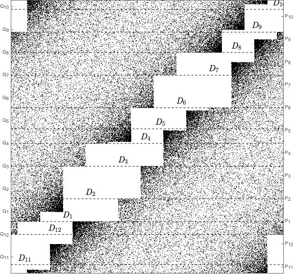
Figure 6. The domain $\Omega_{\,\overline{\!D\!}\,}$ for the parameters ${\,\overline{\!D\!}\,}$ in (22).

The following section gives six types of extremal parameter choices whose duals can be described easily for any genus.

Proposition 25.

For any $g\geq 2$,

1. ${\,\overline{\!P\!}\,}$ and $\,\overline{\!Q\!}\,$ are dual to each other.

2. $\{P_{1},Q_{2},P_{3},Q_{4},\ldots\}$ and $\{Q_{1},P_{2},Q_{3},P_{4},\ldots\}$ are dual to each other.

3. $\{P_{1},P_{2},Q_{2},Q_{2},P_{3},P_{4},Q_{5},Q_{6},\ldots\}$ is dual to itself.

4. $\{Q_{1},Q_{2},P_{2},P_{2},Q_{3},Q_{4},P_{5},P_{6},\ldots\}$ is dual to itself.

The duality of the classical cases $\,\overline{\!P\!}\,$ and $\,\overline{\!Q\!}\,$ is shown in [4]. The domains for the other four parameters choices are shown for genus $g=2$ in [1, Figure 12].

Proof of 25(b).

Let $A_{i}=P_{i}$ for odd $i$ and $A_{i}=Q_{i}$ for even $i$. When $i$ is odd, (8) and the definition of $\sigma$ from (2) give that $G_{4g-i}=T_{i}G_{i-2}$. Setting $j=\sigma(i-2)=4g-(i-2)=4g+2-i$, which is also odd, we also get that $G_{\sigma(j)}=T_{j}G_{j-2}$, or, equivalently, $G_{i-2}=T_{4g+2-i}G_{4g-i}$. Therefore

$$G_{i-2}=T_{4g+2-i}G_{4g-i}=T_{4g+2-i}(T_{i}G_{i-2})=T_{\sigma(i-2)}T_{i}G_{i-2}.$$

The fixed points of $T_{\sigma(i-2)}T_{i}$ are $P_{i-1}$ and $Q_{i}$, and since $G_{i-2}\in[P_{i-2},P_{i-1}]$, we have that $G_{i-2}=P_{i-1}$. Since this holds for all even $i$, we can reindex to say that

$$G_{i}=P_{i+1}\qquad\text{for $i$ odd.}$$

For $k$ even, (8) and (2) and (7) give that $G_{2-k}=T_{k+4g-1}G_{k+4g-2}$ and that $G_{k+4g-2}=T_{3-k}G_{2-k}$, so

$$G_{2-k}=T_{k+4g-1}T_{3-k}G_{2-k}=T_{\tau(k)+1}T_{\sigma(k)+1}G_{2-k},$$

and since the fixed points of $T_{\tau(k)+1}T_{\sigma(k)+1}$ are $P_{\sigma(k)}$ and $Q_{\sigma(k)+1}$, we must have $G_{2-k}=G_{\sigma(k)}=P_{\sigma(k)}=P_{2-k}$. Reindexing to $i=2-k$, we have that

$$G_{i}=P_{i}\qquad\text{for $i$ even.}$$

Having determined $G_{1},\ldots,G_{8g-4}$, we use (13) to compute that

$$D_{i}=T_{\tau\sigma(i)+1}G_{\tau\sigma(i)}=\left\{\begin{array}[]{ll}T_{\tau\sigma(i)+1}P_{\tau\sigma(i)+1}&\text{if $i$ odd}\\ T_{\tau\sigma(i)+1}P_{\tau\sigma(i)}&\text{if $i$ even}.\end{array}\right.$$

In general $T_{\tau\sigma(i)+1}P_{\tau\sigma(i)+1}=Q_{i}$ and $T_{\tau\sigma(i)+1}P_{\tau\sigma(i)}=P_{i}$, so this gives exactly ${\,\overline{\!D\!}\,}=\{Q_{1},P_{2},Q_{3},P_{4},Q_{5},\ldots\}$ as the dual to ${\,\overline{\!A\!}\,}=\{P_{1},Q_{2},P_{3},Q_{4},\ldots\}$. ∎

References

- [1] A. Abrams, S. Katok. Adler and Flatto revisited: cross-sections for geodesic flow on compact surfaces of constant negative curvature, Studia Mathematica 246 (2019), 167–202.
- [2] A. Abrams, S. Katok, I. Ugarcovici. Flexibility of entropy of boundary maps for surfaces of constant negative curvature. Submitted to Ergodic Theory and Dynamical Systems, September 2019. arxiv.org/abs/1909.07032
- [3] R. Adler. Symbolic dynamics and Markov partitions, Bull. Amer. Math. Soc. 35 (1998), No. 1, 1–56.
- [4] R. Adler, L. Flatto. Geodesic flows, interval maps, and symbolic dynamics, Bull. Amer. Math. Soc. 25 (1991), No. 2, 229–334.
- [5] J. Birman, C. Series. Dehn’s algorithm revisited, with applications to simple curves on surfaces, Combinatorial Group Theory and Topology (AM-111), Princeton University Press, (1987), 451–478.
- [6] F. Bonahon. The geometry of Teichmüller space via geodesic currents, Inventiones Mathematicae 92 (1988), 139–162.
- [7] R. Bowen, C. Series. Markov maps associated with Fuchsian groups, Inst. Hautes Études Sci. Publ. Math. 50 (1979), 153–170.
- [8] A. Katok, B. Hasselblatt. Intro. to the Modern Theory of Dynamical Systems, Cambridge University Press, 1995.
- [9] S. Katok. Coding of closed geodesics after Gauss and Morse. Geom. Dedicata 63 (1996), 123–145.
- [10] S. Katok, I. Ugarcovici. Structure of attractors for -continued fraction transformations. Journal of Modern Dynamics 4 (2010), 637–691.
- [11] S. Katok, I. Ugarcovici. Applications of -continued fraction transformations. Ergodic Theory and Dynamical Systems 32 (2012), 755–777.
- [12] S. Katok, I. Ugarcovici. Structure of attractors for boundary maps associated to Fuchsian groups, Geometriae Dedicata 191 (2017), 171–198.
- [13] S. Katok, I. Ugarcovici. Errata: Structure of attractors for boundary maps associated to Fuchsian groups, Geometriae Dedicata 198 (2019), 189–181.
- [14] P. Koebe. Riemannsche Mannigfaltigkeiten und nicht euklidische Raumformen, IV, Sitzungsberichte Deutsche Akademie von Wissenschaften, (1929), 414–557.
- [15] B. Weiss. On the work of Roy Adler in ergodic theory and dynamical systems, in Symbolic dynamics and its applications (New Haven, CT, 1991), 19–32, Contemp. Math. 135, Amer. Math. Soc., Providence, RI, 1992.