Gravitating superconducting solitons in the (3+1)-dimensional Einstein gauged non-linear $\sigma$-model

Abstract

In this paper, we construct the first analytic examples of $(3+1)$-dimensional self-gravitating regular cosmic tube solutions which are superconducting, free of curvature singularities and with non-trivial topological charge in the Einstein-$SU(2)$ non-linear $\sigma$-model. These gravitating topological solitons at a large distance from the axis look like a (boosted) cosmic string with an angular defect given by the parameters of the theory, and near the axis, the parameters of the solutions can be chosen so that the metric is singularity free and without angular defect. The curvature is concentrated on a tube around the axis. These solutions are similar to the Cohen-Kaplan global string but regular everywhere, and the non-linear $\sigma$-model regularizes the gravitating global string in a similar way as a non-Abelian field regularizes the Dirac monopole. Also, these solutions can be promoted to those of the fully coupled Einstein-Maxwell non-linear $\sigma$-model in which the non-linear $\sigma$-model is minimally coupled both to the $U(1)$ gauge field and to General Relativity. The analysis shows that these solutions behave as superconductors as they carry a persistent current even when the $U(1)$ field vanishes. Such persistent current cannot be continuously deformed to zero as it is tied to the topological charge of the solutions themselves. The peculiar features of the gravitational lensing of these gravitating solitons are shortly discussed.

I Introduction

Topological defects are formed in phase transitions when a system goes from a state of higher symmetry to a state of lower symmetry. They can be classified as local or global depending on the fact if a local or global symmetry is broken. Topological defects occur in very different areas of physics like, for example, condensed matter physics, high energy physics, and cosmology. In condensed matter physics perhaps the most famous and intuitive example is the formation of domain walls in ferromagnetic materials, which separate domains with different magnetization. Another famous example is the formation of vortex lines in superfluid helium and line defects (dislocations) in crystals. A topological defect can sometimes be completely regular in which case it is known as a topological soliton. They play a fundamental role in quantum field theory, nuclear physics, and high energy physics 1 , 2 .

The first example of stable topological soliton in three space dimensions was proposed by Skyrme and it is known as Skyrmion skyr . It has the remarkable property of possessing Fermionic excitations despite the fact that the dynamical field is an $SU(2)$-valued scalar field. At leading order in the ’t Hooft large N expansion 5 , 6 , 7 , the Skyrme model represents a (phenomenologically successful) low energy description of Quantum Chromodynamics (QCD).

The Skyrme model arose from a clever modification of the non-linear $\sigma$-model (NLSM henceforth), which is the low energy description of the dynamics of Pions (for nice reviews see e.g. 3 , 4 ). The Skyrme term was added to the NLSM in order to avoid Derrick’s no-go scaling argument 8 preventing the existence of static soliton solutions of finite energy. On the other hand, it should be kept in mind that the elegant arguments in 9 (see also 11 , 12 , 13 , 14 , and references therein) to show that Skyrmions represent Fermions (at least semi-classically) are only based on the existence of stable solitons with non-trivial third homotopy class while they do not use directly the Skyrme term in itself. Thus, it is extremely interesting to search for alternative ways to avoid Derrick’s scaling argument in order to achieve “Fermions out of Bosons” with the simplest possible ingredients. The main approaches to avoid the no-go scaling argument in 8 are, first of all, to minimally couple the NLSM to gravity and/or to Maxwell theory. Indeed, using the techniques developed in canfora2 , 56 , 56b , 58 , 58b , ACZ , Ayon2 , CanTalSk1 , canfora10 , Giacomini:2017xno , ACLV , Fab1 , gaugsk , Canfora:2018clt , lastEPJC , crystal1 , crystal2 , exact self-gravitating NLSM solutions with non-trivial topological charge have been found in CDP , CDGP and GO . Secondly, it is very helpful to construct time-dependent ansatz for the $SU(2)$-valued matter field with the property that the energy-momentum tensor is time-independent (this idea is the $SU(2)$ generalization of the Bosons star ansatz for a $U(1)$-charged scalar field: see 62 , 63 and references therein). Such a generalization has been achieved in ACZ , Ayon2 , Fab1 , crystal1 and crystal2 .

Further relevant topological solitons which play an important role in high energy as well as condensed matter physics, are the Abrikosov-Nielsen-Olesen vortex line abrikosov , Nie-Ole and the ’t Hooft-Polyakov monopole in the $SU(2)$ Yang-Mills-Higgs system thooft , polyakov . It is worth to mention that the latter at large distances looks like a Dirac monopole, however, the Dirac monopole, which describes a point-like magnetic charge, is singular at the origin whereas the ’t Hooft-Polyakov monopole is regular at the origin.

The formation of topological defects are very important in grand unified theories as the actual symmetry group of the standard model is supposed to be a result of a series of spontaneous symmetry breaking of a larger symmetry group. This means that topological defects play a fundamental role from microscopic scale to extremely large scale namely in cosmology due to the fact that the universe in its evolution expanded and cooled down, and therefore went through several phase transitions were topological defects have formed. As in cosmology, the most relevant interaction is gravity, the topological defects must be studied in the context of field theories coupled to gravity.

In cosmology the topological defects which attracted the most attention of the scientific community are the cosmic strings. The simplest exact cosmic string solution is given by an energy-momentum tensor concentrated in a line vilenkin1 (for example the $z$ axis)

$$T_{\alpha\beta}\ =\ \mu\delta(x)\delta(y)\mathrm{diag}(1,0,0,1)\ .$$ (1)

The exact solution of the Einstein field equations associated with this energy-momentum tensor, written in cylindrical coordinates, is locally but not globally flat

$$ds^{2}=-dt^{2}+dr^{2}+r^{2}d\theta^{2}+dz^{2}\ ,$$ (2)

as the range of the angular coordinate $\theta$ is not, as usual, $2\pi$ but

$$0\leq\theta\leq 2\pi(1-4G\mu)\ ,$$ (3)

where $G$ and $\mu$ are the gravitational constant and the mass of the cosmic string per unit length, respectively. Therefore, this locally flat space-time has a conical defect, an angular deficit $\Delta=8G\mu$ and has a curvature singularity on the $z$ axis. A possible way to smooth out the singularity is to smear the energy-momentum tensor on a cylinder of finite radius $\delta$ and it is possible to find exact solutions gott , hiscock , linet . The principal problem of this procedure is that there is a sharp boundary whose radius is arbitrary and moreover the energy-momentum tensor is not derived from some fundamental action principle.

In order to find a cosmic string solution from a fundamental action principle usually the Einstein-Yang-Mills-Higgs action is used, but unfortunately no exact solutions are known. An explicit gravitating global cosmic string metric (where the fundamental field is a Goldstone boson instead of the Higgs and Yang-Mills fields) was found by Cohen and Kaplan, and has the peculiarity that the matter distribution has no sharp boundary and the angular defect varies with the distance from the symmetry axis cohen-kaplan . This metric has a curvature singularity at a finite distance from the axis. It was shown that non-singular gravitating global strings can exist if there is an explicit time dependence in the metric gregory , draper . For a nice explanation of the properties of the Cohen-Kaplan global string see e.g. bookVS pages 196-198.

The existence of cosmic strings has many important cosmological and astrophysical implications. For example, cosmic strings have been proposed to have a role in the galaxy formation as a source of density perturbations kibble . Cosmic strings have also observable effects through gravitational lensing being the most known effect the formation of double images vilenkin1 , vilenkin3 , gott2 . It is worth to point out that the space-time generated by a thin string (with a Dirac delta matter source) does not exert force on a test particle being locally flat, but the existence of a conical defect still generates double images. Perhaps one of the most fascinating aspects of cosmic strings is that, under certain conditions, they become superconducting as it was shown in the pioneering article of Witten wittenstrings . This can have observable effects as such superconducting strings would act as sources of synchrotron radiation or high energy cosmic rays vilenkin2 . Moreover, it has also been proposed that superconducting strings moving in a magnetized plasma can be a mechanism for the production of gamma-ray bursts BHV .

Due to the many important cosmological and astrophysical implications of cosmic strings, it is of great interest to find analytic non-singular solutions that can be derived from some fundamental action principle which leaves no arbitrariness in the choice of fields and their potentials. Indeed, as it has been explained before, in the case of the Einstein-Yang-Mills-Higgs action no such exact solutions are known. The known exact solutions are the thin string with Dirac delta matter source and the global string, both of them possess curvature singularities which would go against the cosmic censorship conjecture. An important point is how to choose a fundamental matter field. Here we will consider the (gauged) NLSM as it is an effective low energy description of the dynamics of Pions (as well as of their electromagnetic properties).

In this paper, we construct the first examples of analytic and singularity free cosmic tube solutions for the self-gravitating $SU(2)$-NLSM. At large distance the metric behave in a similar way to the one of a cosmic string boosted in the axis and has an angular defect related to the parameter of the theory, however near the axis the parameter of the solution can be chosen in such way that the solution is free of singularities and without angular defect. This means that these solutions are free of singularities everywhere and the angular defect depends on the distance from the axis. It is also worth pointing out that the matter field does not have a sharp boundary and the curvature reaches its maximum on a tube around the axis rather than on the axis itself. All these features make the new solutions similar to a global string with the big difference that they are regular instead of having a singularity at finite distance from the axis. The cosmic tubes found here are related to global strings in the same way as non-Abelian monopole are related to Dirac monopoles. In other words, the NLSM regularizes the global string keeping a similar behavior at large distances. Another relevant feature of the solutions presented here is that these possess non-trivial topological charge (the third homotopy class). It is important to mention that in Jackson:1988xk , Jackson:1988ku and Nitta:2007zv , string solutions in the Skyrme model with mass term have been constructed. These configurations were obtained using a static ansatz that facilitates the resolution of the field equations numerically, but that leads to the strings possessing a zero topological density. Those strings, therefore, are classically unstable and are expected to decay into Pions. On the other hand, the temporal dependency in the $U$ field that we introduce, as we will see before, allows us to construct analytical and topologically non-trivial solutions by circumventing Derrick’s theorem (as we have previously pointed out) and without having to include the Skyrme term or additional potentials. Our solutions, having a topological charge, can not decay in the configurations found in Jackson:1988xk , Jackson:1988ku and Nitta:2007zv . Furthermore, these tubes can be promoted to full solutions of the Einstein-Maxwell-NLSM in which the NLSM field is minimally coupled both to the $U(1)$ field as well as to gravity. These gauged solutions carry a persistent current even when the $U(1)$ gauge field is zero and therefore becomes superconducting in the sense of wittenstrings . In particular, the superconducting currents are tied to the topological charge so that they cannot be deformed continuously to zero (that is why they are persistent). It is worth to emphasize that the gravitating solitons constructed in the present paper only involve degrees of freedom arising from low energy QCD minimally coupled with General Relativity (GR) without the need of additional potentials.

I.1 Comparison with Existing Literature

Here it is interesting to compare our novel results with some of the results already existing in the literature. In particular, we will refer to the nice references Jackson:1988xk , Jackson:1988ku , Nitta:2007zv , Volkov1 , Volkov2 , Comtet:1987wi , Moss:1987ka , Babul:1988qt , Zhang:1997is , Balachandran:2001qn , Carter:2002te . Here below we list these four important new features of our solutions (for the sake of clarity, we will call these novel features A, B, C and D).

A) First and foremost, our regular and topologically non-trivial superconducting tubes are also gravitating. Namely, we couple them to the Einstein equations since one of our main goals is to determine the peculiar features of the gravitational field generated by superconducting tubes. The reason is that, as it was already clarified in Witten’s original reference, the spectacular observational effects of superconducting tubes appear in situations in which the gravitational field should not be neglected. Moreover (for the reasons explained here below in point B) we are willing to construct such gravitating superconducting tubes analytically rather than numerically. On the other hand, many of the relevant examples of superconductive tubes available in the literature are numerical and found in flat space-times (such as the examples in the very nice references Jackson:1988xk , Jackson:1988ku , Nitta:2007zv , Volkov1 , Volkov2 , Balachandran:2001qn ).

B) The second main novel feature is that our regular gravitating solitons in a sector with non-vanishing topological charge are completely analytic: to the best of our knowledge, all the most relevant examples available in the literature are numerical. An obvious question is: why should one insist so much on finding analytic solutions if these equations can be solved numerically? Indeed, very powerful numerical techniques are available in the literature to analyze gravitating superconducting tubes (as, for instance, in Jackson:1988xk , Jackson:1988ku , Nitta:2007zv , Volkov1 , Volkov2 , Comtet:1987wi , Moss:1987ka , Babul:1988qt , Zhang:1997is , Balachandran:2001qn , Carter:2002te ). There are many sound reasons to strive for analytic solutions even when numerical techniques are available (especially when, as in the present paper, one is working in $(3+1)$-dimensions). Here below we will list two of them which are quite relevant for the present analysis. First of all, as general motivation, it could be enough to remind all the fundamental concepts that we have understood thanks to the availability of the Schwarzschild and Kerr solutions in GR and of the non-Abelian monopoles and instantons in Yang-Mills-Higgs theory. Much of what we now know about black hole physics in GR and instantons and monopoles in gauge theories arose from a careful study of the available analytic solutions. Hence, a systematic tool to construct analytic gravitating superconducting tubes can greatly enlarge our understanding of these very important topological defects. Secondly, the analytic knowledge of these configurations greatly simplifies the gravitational lensing analysis (indeed, it is worth emphasizing that gravitational lensing is the main phenomenological tool with which one can discover such objects).

C) The third novel feature of our gravitating superconducting tubes is that they are constructed entirely in the low energy limit of QCD minimally coupled both to GR and to Maxwell theory. Indeed, at leading order in the large N limit, the $SU(2)$ NLSM is the low energy limit of QCD describing the dynamics of Pions (and also of Baryons when the topological charge is non-vanishing as in our manuscript). Thus, in particular, our solutions are physically very different from the ones in the two nice references Volkov1 , Volkov2 (which are closely related to the electroweak sector of the standard model). Our solutions instead can be very relevant in situations in which Hadrons interact strongly both electromagnetically and gravitationally. Needless to say, there are many relevant situations from the astrophysical and cosmological point of view where both the electromagnetic and the gravitational interactions with Hadrons cannot be neglected (as it happens, for instance, in the physics of neutron stars). Hence, our solutions are not only of academic interest but they can play an important role in phenomenologically relevant situations.

D) The fourth novel feature of our gravitating superconducting tubes is that the persistent character of the superconductive current is extremely transparent. In particular, we have taken great care to build an ansatz with the following properties. Firstly, we want a consistent ansatz with a non-vanishing topological charge (which, in our case, is interpreted as the Baryonic charge of the configuration) because configurations with non-vanishing topological charge cannot decay into the trivial configurations (neither, in fact, into configurations with different topological charges). Secondly, we want a consistent ansatz in which the electromagnetic current is protected by topology (for instance, the numerical solutions constructed in the nice references by Nitta-Shiki and Jackson have vanishing topological charge Jackson:1988xk , Jackson:1988ku , Nitta:2007zv ). Thirdly, we need a time-dependent ansatz (in order to avoid the Derrick scaling argument: see Rosen:1968 , Friedberg:1979 and Coleman:1985 .) which is, at the same time, compatible with a stationary metric and carries a non-trivial topological charge.

In other words, the electromagnetic current associated with our configurations is proportional to the topological density of the configurations themselves. The physical consequence of this fact is that our current cannot be deformed continuously to the trivial vanishing current as this would imply also a jump in the topological charge. However, there is no continuous deformation that can change the topological charge. It is worth to emphasize that the energy scale of GUT symmetry breaking is $10^{15}$ GeV while the non-linear $\sigma$-model considered in the present manuscript is motivated as a low-energy effective theory of QCD, is relevant at much lower energy scales. On the other hand, the superconducting nature of the gravitating solitons to be constructed here below may strongly affect the scattering of electromagnetic waves leading to potentially visible effects. The reason is that gravitational lensing does not take into account the very strong interactions of the electromagnetic field with the matter field. Unfortunately, we cannot be precise yet since the problem of the scattering of electromagnetic waves in these gravitating solitons background must be solved numerically. We hope to come back to this interesting point in a future publication. Therefore, our superconducting currents are entirely protected by topology and they cannot decay; these are genuine persistent (and, therefore, superconductive) currents. Moreover, in the original Witten’s reference, superconducting currents can only appear when suitable inequalities on the parameters of the Higgs potential are satisfied. In our case instead we do not need any potential at all; it is just the topology of the low energy limit of QCD which keeps the currents alive forever without any extra ingredient.

The structure of the paper is the following: in Sections II and III, we present the model, give our ansatz and the corresponding field equations. In Section IV we construct the exact regular cosmic tube solutions of the Einstein $SU(2)$-NLSM and show that they possess non-trivial topological charge. Also we study the geodesic equations and their main physical properties. In Section V it will be shown how to promote the found configurations to be solutions of the gauged Einstein NLSM system and how these are superconducting configurations. In Section VI we discuss the flat limit of our configurations. In the last Section, our conclusions are detailed.

II The Einstein $SU(2)$-NLSM

The Einstein-NLSM theory is described by the action

$$I[g,U]=\int d^{4}x\sqrt{-g}\left(\frac{\mathcal{R}}{2\kappa}+\frac{K}{4}\mathrm{Tr}[L^{\mu}L_{\mu}]\right),$$ (4)

where $\mathcal{R}$ is the Ricci scalar and $L_{\mu}$ are the Maurer-Cartan form components $L_{\mu}=U^{-1}\partial_{\mu}U$ for $U(x)\in SU(2)$. Here $\kappa$ is the gravitational constant and the positive coupling $K$ is fixed by experimental data. In our convention $c=\hbar=1$ and Greek indices run over the four dimensional space-time with mostly plus signature. In this paper, we follow a standard convention that the Riemann curvature tensor, the Ricci tensor, and the Ricci scalar are given by

$$R^{\alpha}_{\phantom{\alpha}\beta\mu\nu}=\Gamma^{\alpha}_{\phantom{\alpha}\beta\nu,\mu}-\Gamma^{\alpha}_{\phantom{\alpha}\beta\mu,\nu}+\Gamma^{\alpha}_{\phantom{\alpha}\rho\mu}\Gamma^{\rho}_{\phantom{\rho}\beta\nu}-\Gamma^{\alpha}_{\phantom{\alpha}\rho\nu}\Gamma^{\rho}_{\phantom{\rho}\beta\mu}\ ,$$

$$R_{\mu\nu}=R^{\alpha}_{\phantom{\alpha}\mu\alpha\nu}\ ,\qquad\mathcal{R}=g^{\mu\nu}R_{\mu\nu}\ ,$$

respectively.

In order to produce a correct physical interpretation of the topological solitons constructed here and compare with the cosmic string solutions already existing in the literature, in this work we will refer to configurations with vanishing cosmological constant, however the techniques used here are also effective in presence of a cosmological constant. We hope to come back on this interesting issue in a future publication.

The complete Einstein-NLSM equations read

$$\nabla^{\mu}L_{\mu}=0\ ,\qquad G_{\mu\nu}=\kappa T_{\mu\nu}\ ,$$ (5)

where $G_{\mu\nu}$ is the Einstein tensor and $T_{\mu\nu}$ the energy-momentum tensor of the NLSM given by

$$T_{\mu\nu}=-\frac{K}{2}\mathrm{Tr}\left[L_{\mu}L_{\nu}-\frac{1}{2}g_{\mu\nu}L^{\alpha}L_{\alpha}\right].$$ (6)

The winding number of the configurations reads

$$w_{\text{B}}=\frac{1}{24\pi^{2}}\int\rho_{\text{B}}\ ,\quad\rho_{\text{B}}=\text{Tr}[\epsilon^{ijk}L_{i}L_{j}L_{k}]\ .$$ (7)

When the topological density $\rho_{\text{B}}$ is integrated on a space-like surface $w_{\text{B}}$ represents the Baryon number. We will only consider configurations in which $\rho_{\text{B}}\neq 0$.

To construct analytical solutions in this theory we will use the generalized hedgehog ansatz (see canfora2 , 56 , 56b , 58 , 58b , ACZ , Ayon2 , CanTalSk1 , canfora10 , Giacomini:2017xno , ACLV , Fab1 , gaugsk , Canfora:2018clt , lastEPJC , crystal1 , crystal2 ), which is defined as

$$U^{\pm 1}(x^{\mu})=\cos\left(\alpha\right)\mathbf{1}_{2}\pm\sin\left(\alpha\right)n^{i}t_{i}\ ,\ \ \ \ n^{i}n_{i}=1\ ,$$ (8)

$$n^{1}=\sin\Theta\cos\Phi\ ,\ \ \ n^{2}=\sin\Theta\sin\Phi\ ,\ \ \ n^{3}=\cos\Theta\ ,$$

where $t_{i}\equiv i\sigma_{i}$, with $\sigma_{i}$ are the Pauli matrices. It should be noticed that the Maurer-Cartan forms are adapted for the process of solving the field equations, since they satisfy the $SU(2)$ algebra. The choice of the ansatz in Eq. (8) is adapted to the commutation relations of the Maurer-Cartan form in such a way to simplify as much as possible the corresponding Einstein equations (as it will be discussed in a moment). A necessary (but, in general, not sufficient) condition in order to have non-vanishing topological charge is

$$d\alpha\wedge d\Theta\wedge d\Phi\neq 0\ ,\qquad\Longleftrightarrow\qquad\epsilon^{ijk}(\partial_{i}\alpha)(\partial_{j}\Theta)(\partial_{k}\Phi)\neq 0\ ,$$ (9)

where $\alpha$, $\Theta$ and $\Phi$ are the three scalar degrees of freedom appearing in the standard parametrization of the $SU(2)$-valued scalar field defined in Eq. (8).

III Ansatz and Field Equations

The ansatz in Eq. (8) is defined over the Weyl-Lewis-Papapetrou metric

$$ds^{2}=-\frac{B_{0}^{2}\omega_{s}}{e^{f_{0}}}\Big{(}\frac{2e^{f_{0}}}{B_{0}}-\omega_{s}G\Big{)}dt^{2}-\frac{2B_{0}^{2}}{e^{f_{0}}}\Big{(}\frac{e^{f_{0}}}{B_{0}}-\omega_{s}G\Big{)}dtdz+\frac{B_{0}^{2}}{e^{f_{0}}}Gdz^{2}+e^{-2R}\big{(}dX^{2}+d\theta^{2}\big{)}\ ,$$ (10)

with $G=G(X,\theta)$, $R=R(X)$, while $B_{0}$, $\omega_{s}$, $f_{0}$ are arbitrary constants. Since the metric determinant of the section spanned by $t$ and $z$ is negative definite (and $e^{-2R}$ is definite positive as we will show in the next sections),

$$\begin{vmatrix}g_{tt}&g_{tz}\\ g_{zt}&g_{zz}\end{vmatrix}=-B_{0}^{2}<0\ ,$$ (11)

the space-time with this metric is always Lorentzian regardless of the metric components in the $t-z$. As it will be discussed in the next sections, in order to have an integer value of the topological charge, one must allow the whole range of real number as the domain of the coordinate $X$:

$$-\infty<X<\infty\ ,$$ (12)

and $\theta$ is an angular coordinate with range

$$\theta\in[0,2\pi]\ .$$

According to crystal1 , crystal2 we will consider a matter field in the form

$$\alpha=\alpha(X)\ ,\qquad\Theta=q\theta\ ,\qquad\Phi=\omega_{s}t+z\ .$$ (13)

In Appendix A we have given a detailed explanation of how the above ansatz can be constructed in a systematic way and why it is so effective in the case of the gauged gravitating NLSM. Note that the ansatz defined here above satisfies the necessary condition in Eq. (9) in order to possess a non-trivial topological charge. The sufficient conditions will be discussed in the following sections.

This ansatz is very useful for (at least) three reasons. The first one is because Eq. (13) implies the relations

$$\nabla_{\mu}\Phi\nabla^{\mu}\Phi=0\ ,\qquad\nabla_{\mu}\Theta\nabla^{\mu}\Phi=0\ ,$$

which simplify greatly the NLSM equations. The second reason is that Eq. (13) allows to avoid the Derrick’s scale argument 8 as it is a time dependent ansatz which, however is compatible with a stationary metric. Thirdly, the three coupled field equations for the NLSM in the metric defined in Eq. (10) reduce to the single second order ODE for $\alpha(X)$:

$$\alpha^{\prime\prime}-\frac{q^{2}}{2}\sin(2\alpha)\ =0\ .$$ (14)

It is important to note that this second order equation for $\alpha(X)$ can be reduced to the following first order equation

$$(\alpha^{\prime})^{2}-q^{2}\sin^{2}{\alpha}\ =E_{0}\ ,$$ (15)

where $E_{0}$ is an integration constant. However, the compatibility with the Einstein equation requires that $E_{0}=0$. This situation is different from what happens in flat space-time, where the integration constant $E_{0}$ can be non-zero, see crystal1 and crystal2 .

Quite remarkably, the Einstein equations with the energy-momentum tensor corresponding to the NLSM configuration defined in Eq. (13) are reduced to only two solvable equations:

$$R^{\prime\prime}-K\kappa q^{2}\sin^{2}{\alpha}\ =\ 0\ ,$$ (16)

$$(\partial_{X}^{2}+\partial_{\theta}^{2})G+2C_{0}\sin^{2}(q\theta)e^{-2R}\sin^{2}{\alpha}\ =\ 0\ ,$$ (17)

where $C_{0}=K\kappa e^{f_{0}}/B_{0}^{2}$. Note that once $R$ and $\alpha$ are solved, $G$ can be obtained directly. In fact, Eq. (17) is nothing but a flat linear Poisson equation in two dimensions in which the source term is known explicitly (as $\alpha(X)$ and $R(X)$ have been determined in Eqs. (14) and (16)). Hence, Eq. (17) can be solved, for instance, using the method of Green’s function. In the next sections we will construct the solution using a direct method. At this point, it is worth to emphasize that the function $G$ depends explicitly on $\theta$. As the coordinate $\theta$ plays the role of an angular coordinate going around the Hadronic tube, the fact that $G$ depends on $\theta$ implies that the present family of gravitating solitons is not axi-symmetric. Indeed, our space-time admits two Killing vectors $\partial_{t}$ and $\partial_{z}$ so that there does not exist any closed curve generated by a spacelike Killing vector. Moreover, a direct computation reveals that the Killing equation associted to the present class of metrics in Eqs. (10) and (13) has no further solution other than the two solutions $\partial_{t}$ and $\partial_{z}$: this means that (due to the presence of the function $G(X,\theta)$) the metric is manifestly not axi-symmetric as, otherwise, $\partial_{\theta}$ would be a Killing field as well.

The physical role of the function $G$ will be discussed in the analysis of the curvature invariants and of the geodesics.

IV Gravitating tubes

In this Section we construct exact regular cosmic tube solutions of the Einstein-NLSM and we study its relevant physical properties.

IV.1 Solving the system

Eqs. (14) and (16) can be solved analytically, and the expressions for $\alpha(X)$ and $R(X)$ are given by

$$\alpha(X)=2\arctan\exp\big{(}qX+C_{1}\big{)}\ ,$$ (18)

$$R(X)=K\kappa\ln\big{(}\cosh(qX+C_{1})\big{)}+C_{2}X+C_{3}\ ,$$ (19)

where $C_{1}$, $C_{2}$ and $C_{3}$ are integration constants. Replacing the above in Eq. (17) we obtain the final equation for $G$,

$$\partial_{X}^{2}G+\partial_{\theta}^{2}G+\frac{2K\kappa}{B_{0}^{2}}e^{-2(C_{2}X+C_{3})+f_{0}}\cosh^{-2(K\kappa+1)}(qX+C_{1})\sin^{2}(q\theta)\ =\ 0\ .$$ (20)

At this point it is important to emphasize that considering only Eqs. (8), (10), (13), (18) and (19) the complete Einstein-NLSM system has been reduced to a single equation for the metric function $G$ given in Eq. (20).

The energy density (measured by a co-moving observer) of these configurations is given by

$$T_{\hat{0}\hat{0}}=K\Big{[}q^{2}e^{2C_{2}X+C_{3}}\operatorname{sech}^{2(1-K\kappa)}(qX+C_{1})+\frac{\omega_{s}e^{f_{0}}}{B_{0}(2e^{f_{0}}-B_{0}\omega_{s}G)}\sin^{2}(q\theta)\operatorname{sech}^{2}(qX+C_{1})\Big{]}\ ,$$ (21)

$$\text{where}\qquad T_{\hat{0}\hat{0}}=\mathbf{T}(\hat{\mathbf{e}}_{0},\hat{\mathbf{e}}_{0})\qquad\text{for}\qquad\hat{\mathbf{e}}_{0}=\frac{1}{\sqrt{-g_{00}}}\partial_{t}\ .$$

Note that we should impose the constraint on the integration constants

$$C_{2}<(1-K\kappa)\ |q|\ ,$$ (22)

to avoid divergence of the energy density at $X\rightarrow\pm\infty$.

IV.2 An analytical solution

Using that $\sin^{2}(x)=(1-\cos(2x))/2$ , Eq. (17) becomes

$$(\partial_{X}^{2}+\partial_{\theta}^{2})G+C_{0}e^{-2R(X)}\sin^{2}{\alpha(X)}-C_{0}\cos(2q\theta)\times e^{-2R(X)}\sin^{2}{\alpha(X)}=0\ .$$ (23)

The function $G$ can be expressed by the sum of two functions $G_{1}(X)$ and $G_{2}(X,\theta)$

$$G(X,\theta)=G_{1}(X)+G_{2}(X,\theta)\ ,$$ (24)

which satisfy

$$\frac{d^{2}G_{1}}{dX^{2}}=-C_{0}e^{-2R(X)}\sin^{2}{\alpha(X)}\ ,$$

$$(\partial_{X}^{2}+\partial_{\theta}^{2})G_{2}=C_{0}\cos(2q\theta)\times e^{-2R(X)}\sin^{2}{\alpha(X)}\ .$$ (25)

The first equation is trivially solved by a double integral with respect to $r$,

$$G_{1}(X)=-C_{0}\int_{-\infty}^{X}dX_{1}\int_{-\infty}^{X_{1}}dX_{2}\ e^{-2R(X_{2})}\sin^{2}{\alpha(X_{2})}\ .$$ (26)

We can solve the equation for $G_{2}$ by separation of variables, obtaining

$$G_{2}(X,\theta)=y\ \psi_{1}(X)\cos(2q\theta)\ ,$$ (27)

for some real constant $y$, and $\psi_{1}(X)$ satisfying

$$\psi_{1}^{\prime\prime}-4q^{2}\psi_{1}=\frac{C_{0}}{y}\times e^{-2R(X)}\sin^{2}{\alpha(X)}\ .$$ (28)

Eq. (28) can be solve in terms of Elliptic Functions using the method of variation of parameters. The solution of the homogeneous equation is

$$\psi_{\text{h}}=a\psi_{\text{h}}^{(1)}+b\psi_{\text{h}}^{(2)}=ae^{2qX}+be^{-2qX}\ ,$$

with $a$, $b$ integration constants. On the other hand, a particular solution can be found through

$$\psi_{\text{p}}=A(X)\psi_{\text{h}}^{(1)}+B(X)\psi_{\text{h}}^{(2)}\ ,$$

where

$$A(X)=\int\frac{-\psi_{\text{h}}^{(2)}P(X)}{W(\psi_{\text{h}}^{(1)},\psi_{\text{h}}^{(2)})}dX\ ,\quad B(X)=\int\frac{\psi_{\text{h}}^{(1)}P(X)}{W(\psi_{\text{h}}^{(1)},\psi_{\text{h}}^{(2)})}dX\ ,$$

here $W(\psi_{\text{h}}^{(1)},\psi_{\text{h}}^{(2)})=-4q$ is the Wronskian, and

$$P(X)=\frac{C_{0}}{y}e^{-2R}\sin^{2}{\alpha}\ .$$

Therefore, the solution of Eq. (28) is the sum of $\psi_{\text{h}}$ and $\psi_{\text{p}}$, namely

$$\psi_{1}\ = \ ae^{2qX}+be^{-2qX}+\frac{C_{0}e^{-2(C_{1}+qX)}\cosh^{-2K\kappa}(C_{1}+qX)}{2yK\kappa q^{2}}$$

$$\times\biggl{(}1+(e^{2(C_{1}+qX)}-1){}_{2}F_{1}[1,-1-K\kappa,1+K\kappa,-e^{2(C_{1}+qX)}]\biggl{)}\ .$$ (29)

IV.3 Regularity

Obviously, the regularity of the metric must be discussed by analyzing the corresponding curvature invariants. Taking into account Eqs. (18) and (19), the Ricci scalar $S$, the Kretschmann scalar, the square of the Ricci tensor and of the Weyl tensor for the metric in Eq. (10) read

$$S=2K\kappa q^{2}e^{2(C_{2}X+C_{3})}\cosh^{2(K\kappa-1)}(qX+C_{1})\ ,\qquad R^{\mu\nu\rho\sigma}R_{\mu\nu\rho\sigma}=S^{2}\ ,\qquad R^{\mu\nu}R_{\mu\nu}=\frac{1}{2}S^{2}\ ,$$

$$C_{\alpha\beta\gamma\delta}C^{\alpha\beta\gamma\delta}=\frac{4K^{2}\kappa^{2}}{3}\Big{[}qe^{C_{2}X+C_{3}}\cosh^{K\kappa-1}(qX+C_{1})\Big{]}^{4}\ ,$$

and are all regular everywhere (in particular, $S$ is regular at $X\rightarrow\pm\infty$) if we impose the following condition on the integration constants:

$$|C_{2}|<(1-K\kappa)\ |q|\ .$$ (30)

One may wonder whether the above condition in Eq. (30) is enough to ensure the regularity of the metric. Indeed, it is possible to compute explicitly the main fourteen curvature invariants that are usually considered in the literature to analyze, in four dimensions, the issue of regularity (see Sneddon , Harvey ). Such invariants are

$$I_{1} =S=R_{\mu}{}^{\mu}=2e^{2R}R^{\prime\prime}\ ,\quad I_{2}=R_{\mu}{}^{\nu}R_{\nu}{}^{\mu}=\frac{1}{2}I_{1}^{2}\ ,\quad I_{3}=R_{\mu}{}^{\nu}R_{\rho}{}^{\mu}R_{\nu}{}^{\rho}=\frac{1}{4}I_{1}^{3}\ ,$$

$$I_{4} =R_{\mu}{}^{\nu}R_{\rho}{}^{\mu}R_{\sigma}{}^{\rho}R_{\nu}{}^{\sigma}=\frac{1}{8}I_{1}^{4},\quad J_{1}=A_{\mu\nu\rho\sigma}g^{\mu\rho}g^{\nu\sigma}=\frac{1}{3}I_{1}^{2}\ ,\quad J_{2}=B_{\mu\nu\rho\sigma}g^{\mu\rho}g^{\nu\sigma}=\frac{1}{18}I_{1}^{3}\ ,$$

$$J_{3} =E_{\mu\nu\rho\sigma}g^{\mu\rho}g^{\nu\sigma}=0\ ,\quad J_{4}=F_{\mu\nu\rho\sigma}g^{\mu\rho}g^{\nu\sigma}=0\ ,\quad K_{1}=C_{\mu\nu\rho\sigma}R^{\mu\rho}R^{\nu\sigma}=\frac{1}{12}I_{1}^{3}\ ,$$

$$K_{2} =A_{\mu\nu\rho\sigma}R^{\mu\rho}R^{\nu\sigma}=\frac{1}{36}I_{1}^{4}\ ,\quad K_{3}=C_{\mu\nu\rho\sigma}Q^{\mu\rho}Q^{\nu\sigma}=\frac{1}{48}I_{1}^{5}\ ,\quad K_{4}=A_{\mu\nu\rho\sigma}Q^{\mu\rho}Q^{\nu\sigma}=\frac{1}{144}I_{1}^{6}\ ,$$

$$K_{5} =D_{\mu\nu\rho\sigma}Q^{\mu\rho}Q^{\nu\sigma}=0\ .$$

with

$$A_{\mu\nu\rho\sigma}=C_{\mu\nu\alpha\beta}C_{\gamma\delta\rho\sigma}g^{\alpha\gamma}g^{\beta\delta}\ ,\quad\quad B_{\mu\nu\rho\sigma}=C_{\mu\nu\alpha\beta}A_{\gamma\delta\rho\sigma}g^{\alpha\gamma}g^{\beta\delta}\ ,$$

$$D_{\mu\nu\rho\sigma}=B_{\mu\nu\rho\sigma}-\frac{J_{2}}{12}(g_{\mu\rho}g_{\nu\sigma}-g_{\mu\sigma}g_{\nu\rho})-\frac{1}{4}J_{1}C_{\mu\nu\rho\sigma}\ ,$$

$$\tilde{D}_{\mu\nu\rho\sigma}=\frac{1}{\sqrt{J_{3}}}D_{\mu\nu\rho\sigma}\ ,\quad\quad E_{\mu\nu\rho\sigma}=C_{\mu\nu\alpha\beta}D_{\gamma\delta\rho\sigma}g^{\alpha\gamma}g^{\beta\delta}\ ,$$

$$F_{\mu\nu\rho\sigma}=C_{\mu\nu\alpha\beta}E_{\gamma\delta\rho\sigma}g^{\alpha\gamma}g^{\beta\delta}\ ,\quad\quad Q_{\mu}{}^{\nu}=R_{\rho}{}^{\nu}R_{\mu}{}^{\rho}\ .$$

The regularity condition at $X\rightarrow\pm\infty$ is the same as in Eq. (30). One may wonder if there exists a divergent higher differential invariant of our space-time, such as $R_{;\mu\nu\cdots}R^{;\mu\nu\cdots}$. A potential source of such divergences is the presence of an anisotropic pressure that is not $C^{1}$ Musgrave:1995 . The energy-momentum tensor of the cosmic tube, however, is smooth everywhere so that such a divergence cannot occur. Thus, all the curvature invariants which can be built from the metric in Eqs. (10) and (19) are regular everywhere if the condition in Eq. (30) on the integration constants holds.

Interestingly enough, the function $G(X,\theta)$ is not relevant at all as far as the regularity of the curvature invariants is concerned. Thus, in particular, the curvature invariants do not depend on $\theta$. This implies that all the curvature invariants have a local regular maximum at finite distance from the axis of the tube (as it will be discussed in the next sections, in this radial coorinate $r$ the axis of the tube is located at $X\rightarrow-\infty$ while the peaks of the curvature invariants are at $X=0$ which is at finite distance from the axis). Since, as it has been already emphasized, the curvature invariants do not depend on $\theta$, the regular peaks of the curvature invariants lie on a ring in the $\left(X-\theta\right)$ plane. Such a ring (which is a tube from a three-dimensional perspective) is also the support of the superconducting currents associated with the present class of gravitating topologically non-trivial solitons.

One can also verify that the space-time is of Petrov type II. One more constraint on the integration constant $C_{2}$ will arise from the analysis of the geodesic in the following sections.

IV.4 Periodicity of $U$ and the topological charge

In this subsection we will discuss a simple but deep property of the $SU(2)$ valued scalar field $U$ which has a very important consequence. First of all, one can notice that when

$$q=\frac{1}{2}+n\ ,$$ (31)

with $n$ an integer, the topological charge is non-zero while, when $q$ is an integer, the topological charge vanishes. This can be seen as follows. The topological density corresponding to the NLSM configuration in Eq. (13) reads

$$\rho_{\text{B}}=\left(12q\sin{q\theta}\sin^{2}{\alpha}\right)\alpha^{\prime}\ .$$

Thus, as the range of $\theta$ is $\left[0,2\pi\right]$, the integral of the above density

$$w_{\text{B}}=\int\rho_{\text{B}}dX\wedge d\theta\wedge dz\ ,$$

is non-zero if and only if Eq. (31) holds. It is also worth to note here that the $z$ coordinate goes along the axis of the tube and along the topological density. Thus, in a sense, the quantity

$$\frac{w_{\text{B}}}{L_{z}}=\int\rho_{\text{B}}dX\wedge d\theta\ ,$$

can be interpreted as the topological charge per unit of length of the tube, with $L_{z}=\int dz$.

Here it is worth to emphasize that, when the condition in Eq. (31) holds, $\theta$ is a proper angular coordinate with range $\left[0,2\pi\right]$. First of all, the metric itself is periodic with period $2\pi$ as it depends on $\theta$ only through the function $G(X,\theta)$. The function $G(X,\theta)$ depends on $\theta$ only through the factor $\cos(2q\theta)$ in Eq. (17). Secondly, the energy-momentum tensor of the $SU(2)$-valued scalar field is also periodic in $\theta$ with the same period $2\pi$ when the condition in Eq. (31) holds.

However, the matrix $U$ itself is not periodic in $\theta$ with the same period $2\pi$ as it reads

$$U\ =\ \begin{pmatrix}\cos{\alpha}+i\sin{\alpha}\cos(q\theta)&ie^{-i(z+\omega t)}\sin{\alpha}\sin{q\theta}\\ ie^{i(z+\omega t)}\sin{\alpha}\sin(q\theta)&\cos{\alpha}-i\sin{\alpha}\cos(q\theta)\ \end{pmatrix}\ .$$

On the other hand, one can be sure that the “lack of periodicity” can be compensated by an internal Isospin rotation since the energy-momentum tensor corresponding to the above NLSM configuration is periodic with the correct $2\pi-$period: indeed, if such “lack of periodicity” could not be compensated by an internal rotation, then the energy-momentum tensor would not have the correct period. Consequently, $\theta$ is a proper angular coordinate with range $\left[0,2\pi\right]$ when $q$ is half-integer.

Thus, as it happens with the spin-from-Isospin effect, the internal symmetry group plays a fundamental role. In that case, the spin-from-Isospin effect is generated by the possibility to require “spherical symmetry up to an internal rotation”. In the present case, the condition that $U$ satisfies periodic boundary conditions up to an Isospin rotation is enough to ensure that $T_{\mu\nu}$ is periodic and $w_{\text{B}}\neq 0$.

IV.5 Coordinate transformation and the asymptotic behavior

To analyze the nature of the metric in Eq. (10), it is convenient to make the following coordinate transformation:

$$r(X)=\int_{-\infty}^{X}e^{-R(y)}dy=\int_{-\infty}^{X}\frac{e^{-C_{2}y-C_{3}}}{\big{(}\cosh(qy+C_{1})\big{)}^{K\kappa}}dy\ .$$ (32)

It is obvious that $r(X)$ increases monotonically as $X$ increases, since

$$\frac{dr}{dX}=\frac{e^{-C_{2}X-C_{3}}}{\big{(}\cosh(qX+C_{1})\big{)}^{K\kappa}}>0\ .$$ (33)

Moreover, to make $r(X)$ well-defined, it is necessary to impose that

$$C_{2}<K\kappa|q|\ .$$ (34)

This assumption gives us the range of $r$ given by

$$-\infty<X<\infty\qquad\Longrightarrow\qquad 0<r<\infty\ .$$ (35)

With this coordinate transformation, the metric becomes,

$$ds^{2}=-\frac{B_{0}^{2}\omega_{s}}{e^{f_{0}}}\Big{(}\frac{2e^{f_{0}}}{B_{0}}-\omega_{s}G\Big{)}dt^{2}-\frac{2B_{0}^{2}}{e^{f_{0}}}\Big{(}\frac{e^{f_{0}}}{B_{0}}-\omega_{s}G\Big{)}dtdz+\frac{B_{0}^{2}}{e^{f_{0}}}Gdz^{2}+dr^{2}+e^{-2\tilde{R}(r)}d\theta^{2}\ ,$$

where $\tilde{R}(r)=(R\circ X)(r)$.

As we will show now, the function $e^{-2\tilde{R}(r)}$ of the new cylindrical radial coordinate $r$ both for $r$ close to zero and for $r\rightarrow\infty$ is proportional to $r^{2}$:

$$e^{-2\tilde{R}(r)}\underset{r\rightarrow 0}{\rightarrow}\Delta_{0}r^{2}\ ,\qquad e^{-2\tilde{R}(r)}\underset{r\rightarrow+\infty}{\rightarrow}\Delta_{\infty}r^{2}\ .\$$

This implies that $\theta$ is an angular coordinate. Consequently, it is very important to determine the coefficients $\Delta_{0}$ and $\Delta_{\infty}$ which determine the effective deficit angles seen from observers “very close to” and “very far from” the axis of the tube, respectively.

Note that we have the following two limits of the function $R$;

$$X\longrightarrow\pm\infty\qquad\Longrightarrow\qquad R\longrightarrow(C_{2}\pm K\kappa|q|)X\ ,$$ (36)

so that we also have

$$X\longrightarrow\pm\infty\qquad\Longrightarrow\qquad e^{-R}\longrightarrow 2^{K\kappa}e^{\mp K\kappa C_{1}-C_{3}}e^{-(C_{2}\pm K\kappa|q|)X}\ .$$ (37)

In the limit of $X\gg X_{+}$ for a sufficiently large $X_{+}\gg 0$, we find that

$$r(X)=r_{1}+\frac{2^{K\kappa}\times e^{-(K\kappa C_{1}+C_{3})}}{-(C_{2}+K\kappa|q|)}\Big{(}e^{-(C_{2}+K\kappa|q|)X}-e^{-(C_{2}+K\kappa|q|)X_{+}}\Big{)}$$

$$\hskip 25.29494pt\approx\frac{2^{K\kappa}\times e^{-(K\kappa C_{1}+C_{3})}}{-(C_{2}+K\kappa|q|)}\times e^{-(C_{2}+K\kappa|q|)X}\ .$$ (38)

Here, we have defined a finite constant

$$r_{1}\equiv\int_{-\infty}^{X_{+}}\frac{e^{-C_{2}y-C_{3}}}{\big{(}\cosh(|q|y+C_{1})\big{)}^{K\kappa}}dy\ ,$$ (39)

and in the last line, we used the assumption that $C_{2}+K\kappa|q|<0$. Thus, we obtain

$$e^{-2R}\approx\big{(}K\kappa|q|+C_{2}\big{)}^{2}r^{2}\ ,\qquad\qquad\text{at}\quad X\gg 1\ .$$ (40)

In a similar way, the limit of $X\ll X_{-}$ for a sufficiently small $X_{-}\ll 0$ is found to be

$$r(X)=r_{2}-\frac{2^{K\kappa}\times e^{K\kappa C_{1}-C_{3}}}{-(C_{2}-K\kappa|q|)}\Big{(}e^{-(C_{2}-K\kappa|q|)X_{-}}-e^{-(C_{2}-K\kappa|q|)X}\Big{)}$$

$$\hskip 25.29494pt\approx\frac{2^{K\kappa}\times e^{K\kappa C_{1}-C_{3}}}{-(C_{2}-K\kappa|q|)}\times e^{-(C_{2}-K\kappa|q|)X}\ .$$ (41)

Here, we also have defined a finite constant

$$r_{2}\equiv\int_{-\infty}^{X_{-}}\frac{e^{-C_{2}y-C_{3}}}{\big{(}\cosh(|q|y+C_{1})\big{)}^{K\kappa}}dy\ ,$$ (42)

and in the last line we have used the fact that $X\ll X_{-}\ll 0$. Therefore, we get

$$e^{-2R}\approx\big{(}K\kappa|q|-C_{2}\big{)}^{2}r^{2}e^{-2C_{3}}\ ,\qquad\qquad\text{at}\quad X\ll 0\ .$$ (43)

Now, we see that we can choose $C_{3}$ such that the angular deficit is $1$ near the axis defined by $r(X)=0$ so that $\theta$ becomes a proper angular coordinate. The ratio of the values of $g_{\theta\theta}$ at two infinities becomes,

$$\frac{g_{\theta\theta}(X=\infty)}{g_{\theta\theta}(X=-\infty)}=\frac{g_{\theta\theta}(r=\infty)}{g_{\theta\theta}(r=0)}=\Big{(}\frac{K\kappa|q|+C_{2}}{K\kappa|q|-C_{2}}\Big{)}^{2}<1\ .$$ (44)

When we assume that $G$ dies out at spatial infinity, as supported by the plot given in Fig. 2, the asymptotic form of the metric is found to be

$$ds^{2}=-\frac{B_{0}}{2\omega_{s}}\big{(}2\omega_{s}dt+dz\big{)}^{2}+\frac{B_{0}}{2\omega_{s}}dz^{2}+dr^{2}+\Big{(}\frac{K\kappa|q|+C_{2}}{K\kappa|q|-C_{2}}\Big{)}^{2}r^{2}d\theta^{2}\ ,$$ (45)

which describes a boosted cosmic string at spatial infinity.

IV.6 Geodesics

Let $\lambda$ be an affine parameter of geodesics in our space-time. The geodesic equations are found to be

$$\ddot{t}-B_{0}e^{-f_{0}}\big{(}\omega_{s}\dot{t}+\dot{z}\big{)}\frac{dG}{d\lambda}=0\ ,$$ (46)

$$\ddot{z}+\omega_{s}B_{0}e^{-f_{0}}\big{(}\omega_{s}\dot{t}+\dot{z}\big{)}\frac{dG}{d\lambda}=0\ ,$$ (47)

$$\ddot{X}-\big{(}\dot{X}^{2}-\dot{\theta}^{2}\big{)}\big{(}C_{2}+K\kappa q\tanh(qX+C_{1})\big{)}$$

$$-\frac{1}{2}B_{0}^{2}\big{(}\omega_{s}\dot{t}+\dot{z}\big{)}^{2}e^{2C_{2}X+2C_{3}-f_{0}}\cosh^{2K\kappa}(qX+C_{1})\partial_{X}G=0\ ,$$ (48)

$$\ddot{\theta}-2\dot{X}\dot{\theta}\big{(}C_{2}+K\kappa q\tanh(qX+C_{1})\big{)}$$

$$-\frac{1}{2}B_{0}^{2}\big{(}\omega_{s}\dot{t}+\dot{z}\big{)}^{2}e^{2C_{2}X+2C_{3}-f_{0}}\cosh^{2K\kappa}(qX+C_{1})\partial_{\theta}G=0\ ,$$ (49)

where

$$\frac{dG}{d\lambda}=\dot{X}\partial_{X}G+\dot{\theta}\partial_{\theta}G\ ,$$ (50)

and the dot denotes the derivative with respect to $\lambda$.

From the first two equations, we obtain

$$\omega_{s}\ddot{t}+\ddot{z}=0\qquad\Longrightarrow\qquad\omega_{s}t+z=a\lambda+b\ ,$$ (51)

$$\ddot{z}-\omega_{s}\ddot{t}+2B_{0}e^{-f_{0}}\omega_{s}(\omega_{s}\dot{t}+\dot{z})\frac{dG}{d\lambda}=0\ ,$$ (52)

for some constants $a$ and $b$.

Then, Eqs. (47), (48), and (49) become

$$\ddot{z}+aB_{0}e^{-f_{0}}\omega\frac{dG}{d\lambda}=0\ ,$$ (53)

$$\ddot{X}-\big{(}\dot{X}^{2}-\dot{\theta}^{2}\big{)}\big{(}C_{2}+K\kappa q\tanh(qX+C_{1})\big{)}$$

$$-\frac{1}{2}B_{0}^{2}a^{2}e^{2C_{2}X+2C_{3}-f_{0}}\cosh^{2K\kappa}(qX+C_{1})\partial_{X}G=0\ ,$$ (54)

$$\ddot{\theta}-2\dot{X}\dot{\theta}\big{(}C_{2}+K\kappa q\tanh(qX+C_{1})\big{)}$$

$$-\frac{1}{2}B_{0}^{2}a^{2}e^{2C_{2}r+2C_{3}-f_{0}}\cosh^{2K\kappa}(qX+C_{1})\partial_{\theta}G=0\ .$$ (55)

On the hypersurface of constant $z$, the Eq. (47) becomes

$$\omega_{s}B_{0}e^{-f_{0}}\omega_{s}\dot{t}\ \frac{dG}{d\lambda}=0\ ,$$ (56)

from which we obtain

$$\frac{dG}{d\lambda}=\dot{X}\partial_{X}G+\dot{\theta}\partial_{\theta}G=0\ .$$ (57)

Then, Eq. (46) becomes

$$\ddot{t}=0\qquad\Longrightarrow\qquad t=\frac{a}{\omega_{s}}\lambda+b\ .$$ (58)

For convenience, let’s put

$$a=\omega_{s}\ ,\qquad b=0\ ,\qquad\text{so that}\qquad t=\lambda\ .$$ (59)

Then, the remaining geodesic equations become

$$\ddot{X}-\big{(}\dot{X}^{2}-\dot{\theta}^{2}\big{)}\big{(}C_{2}+K\kappa q\tanh(qX+C_{1})\big{)}$$

$$-\frac{1}{2}B_{0}^{2}\ \omega_{s}^{2}e^{2C_{2}X+2C_{3}-f_{0}}\cosh^{2K\kappa}(qX+C_{1})\partial_{X}G=0\ ,$$ (60)

$$\ddot{\theta}-2\dot{X}\dot{\theta}\big{(}C_{2}+K\kappa q\tanh(qX+C_{1})\big{)}$$

$$-\frac{1}{2}B_{0}^{2}\omega_{s}^{2}e^{2C_{2}X+2C_{3}-f_{0}}\cosh^{2K\kappa}(qX+C_{1})\partial_{\theta}G=0\ .$$ (61)

Using Eq. (57) in a linear combination $\Big{(}\dot{X}\times(\ref{geodesicr1})+\dot{\theta}\times(\ref{geodesictheta1})\Big{)}$ yields

$$\frac{1}{2}\frac{d}{d\lambda}\big{(}\dot{X}^{2}+\dot{\theta}^{2}\big{)}-\dot{X}\big{(}\dot{X}^{2}+\dot{\theta}^{2}\big{)}\big{(}C_{2}+K\kappa q\tanh(qX+C_{1})\big{)}=0\ ,$$

or equivalently,

$$\frac{d}{d\lambda}\Big{[}\frac{1}{2}\ln\big{(}\dot{X}^{2}+\dot{\theta}^{2}\big{)}-C_{2}X-K\kappa\ln\big{\{}\cosh(qX+C_{1})\big{\}}\Big{]}=0\ .$$ (62)

Thus, for some constant $C_{4}$, we have

$$\dot{X}^{2}+\dot{\theta}^{2}=e^{2(C_{2}X+C_{4})}\cosh^{2K\kappa}(qX+C_{1})\ .$$ (63)

We should assume that

$$C_{2}<-K\kappa\ |q|\ ,$$ (64)

to avoid infinity velocities at large $X$. The line element for the geodesic with constant $z$ is

$$ds^{2}=-\frac{B_{0}^{2}\omega_{s}}{e^{f_{0}}}\Big{(}\frac{2e^{f_{0}}}{B_{0}}-\omega_{s}G\Big{)}dt^{2}+e^{-2R}\big{(}dX^{2}+d\theta^{2}\big{)}\ .$$

Divided by the affine parameter $t$, it can be written as

$$B_{0}\omega_{s}\Big{(}B_{0}\omega_{s}e^{-f_{0}}G-2\Big{)}+e^{-2R}\big{(}\dot{X}^{2}+\dot{\theta}^{2}\big{)}=\frac{ds^{2}}{dt^{2}}\equiv\epsilon\ .$$

By an appropriate rescaling $\epsilon$ becomes $-1$ or $0$ for time-like or null geodesic, respectively. Using Eq. (63), we have

$$e^{-2R}\big{(}\dot{X}^{2}+\dot{\theta}^{2}\big{)}=e^{-2C_{2}X-2C_{3}}\operatorname{sech}^{2K\kappa}\big{(}qX+C_{1}\big{)}\times e^{2(C_{2}X+C_{4})}\cosh^{2K\kappa}(qX+C_{1})=e^{-2C_{3}+2C_{4}}\ .$$

Thus, the line element of the geodesic with constant $z$ gives a relation between constants as follows

$$B_{0}\omega_{s}\Big{(}B_{0}\omega_{s}e^{-f_{0}}G-2\Big{)}+e^{-2C_{3}+2C_{4}}-\epsilon=0\ .$$

Using Eq. (63) in the geodesic equation of $r$, from Eq. (60) one finds that

$$\ddot{X} -2\dot{X}^{2}\big{(}C_{2}+K\kappa q\tanh(qX+C_{1})\big{)}-e^{2C_{2}X}\cosh^{2K\kappa}(qX+C_{1})$$

$$\times\Big{\{}e^{2C_{4}}\big{(}C_{2}+K\kappa q\tanh(qX+C_{1})\big{)}+\frac{1}{2}B_{0}^{2}\omega_{s}^{2}e^{2C_{3}-f_{0}}\partial_{X}G\Big{\}}=0\ .$$ (65)

After solving this equation, one should plug the solution to the equation of motion for $\theta$ in Eq. (61) to find $\theta(t)$. This completes the solving process of the geodesic equations with constant $z$. In principle, this problem can be reduced to an effective one-dimensional Newtonian problem observing that, along the geodesics with constant $z$, one has

$$\dot{X}\partial_{X}G+\dot{\theta}\partial_{\theta}G=0\ \ \Rightarrow\ \ \frac{d\theta}{dr}=-\frac{\partial_{r}G}{\partial_{\theta}G}\ ,$$ (66)

where $G(X,\theta)$ is defined in Eqs. (24), (26) and (29). The reason is that from Eq. (66) one can determine $\theta=\theta\left(X\right)$ along the geodesics with constant $z$. Once $\theta=\theta\left(X\right)$ has been determined, one can insert it into Eq. (63) obtaining a first order Newtonian-like equation of the form

$$\dot{X}^{2} = V_{\text{eff}}\left(X\right)\ ,$$

$$V_{\text{eff}}\left(X\right) = \frac{e^{2(C_{2}X+C_{4})}\cosh^{2K\kappa}(qX+C_{1})}{1+\left(\frac{d\theta}{dX}\right)^{2}}\ .$$

However, Eq. (66) is a quite complicated first order non-autonomous differential equation for $\theta\left(X\right)$ due to the explicit form of $G(X,\theta)$ in Eqs. (24), (26) and (29). The relevant issue of the behavior of geodesics in this family of gravitating solitons deserves a more detailed analysis on which we hope to come back in a future publication.

In the usual case of cosmic strings, the angle defect of gravitational lensing is independent of the initial distance of the particle from the source. But in our case, the distribution of source is smoothly spread out to $X=\infty$, so that the angle defect depends on $X_{0}$, the initial location of geodesic motion. This would be one of the most distinguished properties of our solution.

IV.7 Constraint on integration constant

Combining the regularity conditions on the integration constants in Eqs. (22), (30), (34) and (64) we obtain the following single inequality

$$-(1-K\kappa)\ |q|<C_{2}<-K\kappa\ |q|\ .$$ (67)

Thus, when $C_{2}$ satisfies the above condition and $C_{3}$ is chosen as in Eq. (43) all the curvature invariants of the metric are regular and the geodesics behave in a reasonable way. Note that the experimental value of the Pions coupling constant is such that $0<K\kappa\ll 1$. On the other hand, the integration constant $C_{1}$ is a free parameter which fixes the location of the point about which the profile function $\alpha(X)$ is symmetric.

V Gauged gravitating tubes

In this Section we promote our configurations to be solutions of the Einstein-Maxwell-NLSM system, and also show how these are superconducting gravitating tubes.

V.1 The Einstein-Maxwell-NLSM theory

The action of the $U(1)$ gauged Einsten NLSM theory is

$$I[g,U,A]=\int d^{4}x\sqrt{-g}\left[\frac{\mathcal{R}}{2\kappa}+\frac{K}{4}\mathrm{Tr}\left(L^{\mu}L_{\mu}\right)-\frac{1}{4}F_{\mu\nu}F^{\mu\nu}\right]\ ,$$ (68)

$$L_{\mu}=U^{-1}D_{\mu}U\ ,\ \ \ D_{\mu}=\nabla_{\mu}+A_{\mu}\left[t_{3},\ .\ \right]\ ,\ F_{\mu\nu}=\partial_{\mu}A_{\nu}-\partial_{\nu}A_{\mu}\ .$$ (69)

The respective field equations are

$$D_{\mu}L^{\mu}=0\ ,\qquad G_{\mu\nu}=\kappa(T_{\mu\nu}+\bar{T}_{\mu\nu})\ ,$$ (70)

$$\nabla_{\mu}F^{\mu\nu}=J^{\nu}\ ,$$ (71)

where the current $J^{\mu}$ is given by

$$J^{\mu}=\frac{K}{2}\text{Tr}\left[\widehat{O}L^{\mu}\right]\ ,\qquad\widehat{O}=U^{-1}t_{3}U-t_{3}\ ,$$ (72)

and $\bar{T}_{\mu\nu}$ is the energy-momentum tensor of the Maxwell theory

$$\bar{T}_{\mu\nu}=F_{\mu\alpha}F_{\nu}^{\;\alpha}-\frac{1}{4}F_{\alpha\beta}F^{\alpha\beta}g_{\mu\nu}\ .$$ (73)

Note that in the action in Eq. (68) there is a quadratic term in $A_{\mu}$.

The topological charge in this case Callan is given by

$$w_{\text{B}}=\frac{1}{24\pi^{2}}\int_{\Sigma}\rho_{\text{B}}\ ,$$ (74)

where

$$\rho_{\text{B}}=\epsilon^{ijk}\text{Tr}\biggl{[}\left(U^{-1}\partial_{i}U\right)\left(U^{-1}\partial_{j}U\right)\left(U^{-1}\partial_{k}U\right)-\partial_{i}\left[3A_{j}t_{3}\left(U^{-1}\partial_{k}U+\left(\partial_{k}U\right)U^{-1}\right)\right]\biggl{]}\ .$$ (75)

Note that the second term in Eq. (75), the Callan-Witten term, guarantees both the conservation and the gauge invariance of the topological charge.

V.2 Gravitating tubes coupled to the electromagnetic field

Let’s consider the following Maxwell potential

$$A_{\mu}=\left(u,0,0,\frac{1}{\omega_{s}}u\right)\ ,\qquad u=u(X,\theta)\ ,$$ (76)

together with the metric defined in Eq. (10) and the matter field in Eq. (13). This is a very convenient ansatz crystal1 , crystal2 , because a direct computation reveals that the three field equations for the gauged NLSM reduce (once again) to

$$\alpha^{\prime\prime}-\frac{q^{2}}{2}\sin{2\alpha}=0\ ,$$

so that

$$\alpha(X)=2\arctan(e^{qX+C_{1}})\ .$$ (77)

On the other hand, the four Maxwell equations reduce to just one linear equation:

$$\Delta u-2Ke^{-2R}(\omega_{s}-2u)\sin^{2}{\alpha}\sin^{2}{q\theta}=0\ .$$ (78)

Note that this linear equation for $\Psi=\omega_{s}-2u$ can be easily solved, at least numerically, since $\alpha(X)$ is explicitly known and $R(X)$ can be also determined explicitly. In fact, there are two non-trivial Einstein equations that can be combined to obtain an uncoupled equation for $R$, namely

$$R^{\prime\prime}-\frac{1}{2}K\kappa(\alpha^{\prime 2}+q^{2}\sin^{2}{\alpha})=0\ ,$$

so that, as in the case without Maxwell,

$$R(X)=K\kappa\log(\cosh(qX+C_{1}))+C_{2}X+C_{3}\ ,$$ (79)

and $G$ satisfies the following equation

$$\Delta G+\frac{2\kappa}{B_{0}^{2}\omega_{s}^{2}}e^{f_{0}-2R}\biggl{(}K\sin^{2}{\alpha}\sin^{2}{q\theta}(\omega_{s}-2u)^{2}+e^{2R}(\nabla u)^{2}\biggl{)}=0\ .$$ (80)

Hence, once again, the function $G$ satisfy a flat two-dimensional Poisson equation in which the source is explicitly known. Therefore, once the Maxwell equation in Eq. (78) has been solved, the function $G$ can be determined explicitly using several methods (such as the Green functions).

Resuming, using the ansatz for $U$ and $A_{\mu}$ in Eqs. (13), (76) and for the metric in Eq. (10), the Einstein-Maxwell-NLSM field equations reduce simply to Eqs. (78) and (80), where $\alpha(X)$ and $R(X)$ are in Eqs. (77) and (79). It is worth to emphasize that this is a quite remarkable reduction of such a coupled system of non-linear PDEs in a sector with non-trivial topological charge as the NLSM (which is already a very complicated theory in itself) is coupled directly both to GR and to the $U(1)$ gauge field $A_{\mu}$.

The energy density measured in an orthonormal frame is found to be

$$T_{\hat{0}\hat{0}}= \frac{Ke^{f_{0}}}{2\omega_{s}B_{0}(2e^{f_{0}}-B_{0}\omega_{s}G)}\Biggl{[}2\sin^{2}(q\theta)\operatorname{sech}^{2}(qX+C_{1})(2u-\omega_{s})^{2}$$

$$+e^{2C_{2}X+C_{3}}\cosh^{2K\kappa}(qX+C_{1})\Big{\{}(\partial_{X}u)^{2}+(\partial_{\theta}u)^{2}\Big{\}}\Biggl{]}$$

$$+Kq^{2}e^{2C_{2}X+C_{3}}\operatorname{sech}^{2(1-K\kappa)}(qX+C_{1})\ ,$$ (81)

where we used the tetrad given by

$$\hat{\mathbf{e}}_{0}=\frac{1}{\sqrt{-g_{00}}}\partial_{t}\ .$$

The topological charge density, including the Callan-Witten term, is

$$\rho_{\text{B}}=\partial_{X}\Big{(}6q\big{(}\alpha-\sin\alpha\cos\alpha\big{)}\sin(q\theta)+\frac{12q}{\omega_{s}}\sin\alpha\cos\alpha\sin(q\theta)\cdot u\Big{)}+\partial_{\theta}\Big{(}\frac{12}{\omega_{s}}\cos(q\theta)\cdot u\partial_{X}\alpha\Big{)}\ .$$

The current is given by

$$J_{\mu}=2K\sin^{2}{\alpha}\sin^{2}{q\theta}(\partial_{\mu}\Phi-2A_{\mu})\ ,$$ (82)

and the components of the electric and magnetic fields read

$$E_{X}=-\partial_{X}u\ ,\qquad E_{\theta}=-\partial_{\theta}u\ ,\qquad B_{X}=-\frac{1}{B_{0}}e^{2R}\partial_{\theta}u\ ,\qquad B_{\theta}=\frac{1}{B_{0}}e^{2R}\partial_{X}u\ .$$

The plots here below as well as the review of the Witten construction clearly show why these solutions of the Einsten-Maxwell-NLSM represent regular topologically non-trivial gravitating superconducting tubes.

In order to plot the relevant physical functions we have set our parameters as

$$C_{1}=0\ ,\quad C_{2}=-\frac{1}{50}\ ,\quad C_{3}=0\ ,\quad K=\frac{1}{10}\ ,\quad\kappa=\frac{1}{4}\ ,$$

$$q=\frac{1}{2}\ ,\quad\omega_{s}=1\ ,\quad f_{0}=0\ ,\quad B_{0}=\frac{1}{2}\ .$$ (83)

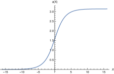
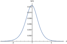
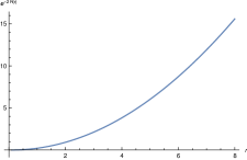
Figure 1: From left to right, the $\alpha$ profile and the Ricci scalar $S$ as functions of the $X$ coordinate and metric function $e^{-2R(r)}$ as a function of the $r$ coordinate.

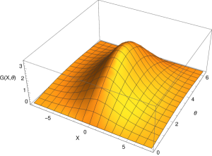
Figure 2: The metric function $G$ as a function of $X$ and $\theta$.

From Fig. 1 and Fig. 2 we can see that even if the metric is not axi-symmetric due to the explicit $\theta$-dependence of $G(X,\theta)$ in Eq. (80), all the curvature invariants are axi-symmetric as they only depend on $X$. Thus, the plots of all the curvature invariants are very similar and they all show a smooth peak at finite distance from the origin (remember that, in the coordinate $X$, the origin is at $X\rightarrow-\infty$). As we expected, $e^{-2R(r)}$ goes as $r^{2}$ when $r\rightarrow 0$ as well as when $r\rightarrow\infty$.

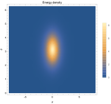
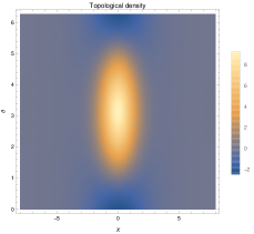
Figure 3: The Energy density $T_{\hat{0}\hat{0}}$ and topological density $\rho_{\text{B}}$ as functions of $X$ and $\theta$.

In Fig. 3, the energy density associated to a comoving observer has two parts. The first one only depends on “$X$” and, as the curvature invariants, has its smooth maximum at the same finite dinstance from the axis. The second part depends both on “$X$” and on “$\theta$” and the corresponding peak is at the same distance from the axis as the peak of the first term and, in $\theta$ is localized around $\theta\sim\pi$. The peaks of the energy density and the peaks of the topological density coincide, as expected.

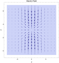
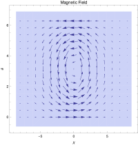
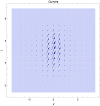
Figure 4: From left to right, the vector density plots of the Electric field $E$, the magnetic field $B$ and of the current $J_{\mu}$.

From the plots in Fig. 4 one can see that $J_{\mu}\neq 0$ only at the position of the two peaks and tends to zero out. Here we have imposed the following boundary conditions,

$$u(X,2\pi)-u(X,0)=0\ ,\quad G(X,2\pi)-G(X,0)=0\ .$$

V.3 Why the tubes are superconductors?

V.3.1 Review of the Witten argument

Before discussing the superconducting nature of the present solutions, we will shortly review the results in wittenstrings (which have been considerably generalized in many subsequent works: see for instance subsequent1 , subsequent2 , subsequent3 , subsequent4 , subsequent5 , subsequent6 , and references therein).

The main motivation to introduce such topological objects is related, of course, to the spectacular observable effects that such objects could have (were they to exist: see the original reference wittenstrings as well as supstr1 , importance1 , importance2 , importance3 , importance4 , importance5 , importance6 , importance7 , new10 , new11 , new12 , new13 , new14 , new15 , new16 , new17 , new18 , new19  and references therein). The second motivation is related to the fact that such remarkable objects can be constructed using quite reasonable ingredients. Many of the examples available in the literature do not use exclusively building blocks within the standard model. For instance, extra $U(1)$ gauge potential as well as Higgs-like scalar fields are often important ingredients while in subsequent1 , subsequent2 , subsequent3 , subsequent4 , subsequent5 , subsequent6 , supersymmetry plays a fundamental role.

The starting point of wittenstrings is the following Lagrangian

$$L_{\text{kin}}=-\frac{1}{4}\left(F^{2}+B^{2}\right)+\left|D\sigma\right|^{2}+\left|D\psi\right|^{2}\ ,$$ (84)

$$F_{\mu\nu}=\partial_{\mu}A_{\nu}-\partial_{\nu}A_{\mu}\ ,\ \ B_{\mu\nu}=\partial_{\mu}S_{\nu}-\partial_{\nu}S_{\mu}\ ,$$

$$D_{\mu}\sigma=\left(\partial_{\mu}+ieA_{\mu}\right)\sigma\ ,\ D_{\mu}\psi=\left(\partial_{\mu}+ieS_{\mu}\right)\psi\ .$$

The above theory has an $U(1)\times U(1)$ gauge symmetry (the first corresponding to $A_{\mu}$ and the second to $S_{\mu}$). In order for the above theory to support superconducting strings, it is necessary to include an interaction potential between the two Higgs fields $\sigma$ and $\psi$. The choice of wittenstrings was

$$V\left(\sigma,\psi\right)=\frac{\lambda}{8}\left(\left|\psi\right|^{2}-\mu^{2}\right)^{2}+\frac{\widetilde{\lambda}}{4}\left|\sigma\right|^{4}+f\left|\sigma\right|^{2}\left|\psi\right|^{2}-m^{2}\left|\sigma\right|^{2}\ ,$$ (85)

$$S_{\text{tot}}=\int d^{4}x\sqrt{g}\left(L_{\text{kin}}+V\left(\sigma,\psi\right)\right)\ .$$ (86)

The reasons behind this choice are the following: The first necessary ingredient is the breakdown of the gauge symmetry corresponding to $S_{\mu}$ in order to ensure the existence of vortices. The Higgs field $\psi$ in the core of the vortex field is usually assumed to only depend on the two spatial coordinates (say, $r$ and $\theta$) transverse to the vortex axis (which is along the $z$-axis). Then, one must require that, in the vacuum, $\left\langle\sigma\right\rangle=0$. At this point, with a clever choice of the range of the parameters of the Higgs potential, one can achieve the following situation. Despite the fact that the (minimization of the) kinetic energy tends to suppress $\left\langle\sigma\right\rangle\neq 0$ within the core, if one chooses $m^{2}$ to be positive, the potential energy will favor $\left\langle\sigma\right\rangle\neq 0$ within the core. As it was shown in wittenstrings , this can indeed happen. In other words, there is an open region in the parameter space in which $\left\langle\sigma\right\rangle=0$ asymptotically but $\left\langle\sigma\right\rangle\neq 0$ within the core of the vortex associated to $\psi$. This is a fundamental technical step since the superconducting currents (to be described in a moment) are sustained by the region in which $\left\langle\sigma\right\rangle\neq 0$. If $\sigma_{0}\left(r,\theta\right)$ minimizes the energy of the string, then the superconducting current is associated with the (slowly varying) phase $\Theta$ of $\sigma_{0}\left(r,\theta\right)$. One can achieve this by introducing the dependence on $z$ and $t$ in $\sigma$ as follows:

$$\sigma\left(r,\theta,z,t\right)=\sigma_{0}\left(r,\theta\right)\exp\left[i\Theta\left(z,t\right)\right]\ .$$ (87)

The expression of the current is

$$\overrightarrow{J}\approx 2e\sigma\left(\overrightarrow{\partial}\Theta+e\overrightarrow{A}\right)\ ,$$ (88)

which is made of two factors. The first factor $\left(\overrightarrow{\partial}\Theta+e\overrightarrow{A}\right)$ is responsible for the dynamics of the zero modes along the strings (associated to the phase $\Theta$). However, such a factor by itself would be “useless” as it needs to “rely on” something. This “something” is the factor $\sigma$. Thus, first of all, the first factor needs $\sigma$ to be different from zero somewhere. For superconducting strings, as it has been already emphasized,  the spatial region where $\sigma\neq 0$ is tube-shaped. However, this is not enough: the configurations in which $\sigma\neq 0$ within a tube-shaped region must be stable, otherwise the current would decay. In the settings of wittenstrings , subsequent1 , subsequent2 , subsequent3 , subsequent4 , subsequent5 , subsequent6 , the linear stability of the configurations where $\sigma\neq 0$ within the string (as well as $\sigma$ approaching to zero outside) were established by direct methods (such as linear perturbation theory). Note also that the current defined above cannot have arbitrarily large values since $\sigma$ has a maximum value determined by the Higgs potential. Once the stability of such tube-shaped regions (which are going to host the superconducting currents) has been established, one can ask:

Under which circumstances the above current is superconducting?

One needs a mechanism that keeps such current perpetually alive even in the absence of an external gauge potential. At this point, topology comes into play. Since $\Theta$ is only defined modulo $2\pi$, the integral over a close loop of the above current will not vanish in general even when one turns off the electromagnetic field. Indeed, one can build a topological invariant associated to (the integral of) $\Theta$. Thus, such a current cannot relax when the topological invariant associated to $\Theta$ is non-zero.

Basic ingredients. A very nice pedagogical construction has been achieved in Shifman:2012vv  where, assuming that symmetry breaking is always generated by suitable Higgs or scalar potentials, the author reduced the basic ingredients to the skeleton. The author required that bulk theory should have an unbroken global non-Abelian symmetry (let us assume, just for concreteness, that such a group is $SU(2)$) allowing the existence of string-like configurations. Moreover, on such string-like configurations, one has to break $SU(2)$ down to a subgroup $U(1)$. As it has been already emphasized, such requirements are usually taken care of by introducing suitable potentials for the scalars. In fact, the Einstein-Maxwell-NLSM has all the above ingredients already “built-in” and there is no need to introduce any potential: the typical interactions among the Maurer-Cartan forms associated to the Isospin degrees of freedom do the job.

Secondly, it would be very nice to use topology not only to ensure the persistent character of the current but also to guarantee the appearance of regions where $\sigma\neq 0$ (such that $\sigma$ approaches zero outside). Higher topological charges can be useful, as we will discuss in the following subsection.

V.3.2 The superconductivity of the tubes

The main features of the above expressions in Eq. (82) for the current of these topologically non-trivial gauged crystals are the following.

1) The current does not vanish even when the electromagnetic potential vanishes ($u=0$).

2) Such a “current left over” $J_{(0)\mu}$:

$$J_{(0)\mu}=2K\sin^{2}(\alpha)\sin^{2}(q\theta)\partial_{\mu}\Phi\ ,$$ (89)

(where $\Phi$ has been defined in Eq. (13)) which survives even when the Maxwell field is turned off, is maximal where the energy density is maximal (namely, where $\sin^{2}(\alpha)\sin^{2}(q\theta)=1$, which defines the positions of the peaks in the energy density as well as in the topological density) and vanishes rapidly far from the peaks.

3) Such residual current $J_{(0)\mu}$ cannot be turned off continuously. This can be seen as follows. There are three ways to “kill” $J_{(0)\mu}$. The first way is to deform $\alpha$ to an integer multiple of $\pi$ (but this is impossible as such a deformation would change the topological charge). The second way is to deform $q\theta$ to an integer multiple of $\pi$ (but also this deformation is impossible due to the conservation of the topological charge). The third way is to deform $\Phi$ to a constant (but also this deformation cannot be achieved). Note also that $\Phi$ is defined modulo $2\pi$ (as the $SU(2)$ valued field $U$ depends on $\cos\Phi$ and $\sin\Phi$ rather than on $\Phi$ itself). This implies that the line integral of $\partial_{\mu}\Phi$ along a closed contour does not necessarily vanish (as it happens in the original Witten argument).

The above characteristics show that the above residual current is a persistent current that cannot vanish as it is topologically protected. This, by definition, implies that $J_{(0)\mu}$ defined in Eq. (89) is a superconducting current supported by the present gauged tubes.

VI The flat limit

In this Section we discuss the flat limit $\kappa\rightarrow 0$ of our solution describing a gauged gravitating soliton. In this limit, the field equations in (14), (16) and (78) become

$$\alpha^{\prime\prime}-\frac{q^{2}}{2}\sin(2\alpha) \ =\ 0\ ,$$ (90)

$$\Delta G \ =\ 0\ ,$$ (91)

$$R^{\prime\prime} \ =\ 0\ ,$$ (92)

$$\Delta u-2Ke^{-2R}(\omega_{s}-2u)\sin^{2}{\alpha}\sin^{2}{q\theta} \ =\ 0\ .$$ (93)

The solutions to the second and third equations are found to be

$$G=0\ ,\qquad R(X)=C_{2}X+C_{3}\ ,$$ (94)

which corresponds to the flat limit of the solution in Eq. (79). When $C_{2}$ does not vanish, the flat limit of the coordinate transformation to the radial coordinate of a cylindrical system in Eq. (32) gives

$$r(X)=\frac{1}{-C_{2}}e^{-C_{2}X-C_{3}}\ ,$$

so that the space-time metric becomes

$$ds^{2}=-d\tilde{t}^{2}+d\tilde{z}^{2}+dr^{2}+C_{2}^{2}r^{2}d\theta^{2}\ ,$$ (95)

where $\tilde{t}=\sqrt{2B_{0}\omega_{s}}t+\sqrt{B_{0}/2}z$, and $\tilde{z}=\sqrt{B_{0}/2}z$. To avoid a conical singularity, we should impose that

$$C_{2}=-1\ .$$ (96)

We have taken the negative value of $C_{2}$ to satisfy the inequality (67). In this cylindrical coordinate system, the equations for $\alpha$ and $u$ become

$$\Big{(}\frac{d^{2}}{dr^{2}}+\frac{1}{r}\frac{d}{dr}\Big{)}\alpha(r)-\frac{q^{2}}{2r^{2}}\sin 2\alpha(r)=0\ ,$$ (97)

$$\Big{(}\frac{\partial^{2}}{\partial r^{2}}+\frac{1}{r}\frac{\partial}{\partial r}+\frac{1}{r^{2}}\frac{\partial^{2}}{\partial\theta^{2}}\Big{)}u(r,\theta)-\frac{8K(\omega_{s}-2u(r,\theta))\sin^{2}{q\theta}}{\big{(}e^{|q|C_{3}+C_{1}}r^{|q|}+e^{-|q|C_{3}-C_{1}}r^{-|q|}\big{)}^{2}}=0\ .$$ (98)

The constraint on the parameters (67) restricts the range of the parameter $q$

$$\frac{1}{1-K\kappa}<|q|<\frac{1}{K\kappa}\ .$$ (99)

It should be noticed that $|q|=1$ is forbidden in the flat spactime limit if $C_{2}\neq 0$. The flat limit of the energy-density is found to be

$$T_{\hat{0}\hat{0}}=\frac{4K\sin^{2}(q\theta)(2u-\omega_{s})^{2}+Kq^{2}/r^{2}}{\big{(}e^{|q|C_{3}+C_{1}}r^{|q|}+e^{-|q|C_{3}-C_{1}}r^{-|q|}\big{)}^{2}}+\frac{K}{2}\Big{(}(\partial_{r}u)^{2}+\frac{1}{r^{2}}(\partial_{\theta}u)^{2}\Big{)}\ ,$$ (100)

where $\hat{\mathbf{e}}_{0}=\partial/\partial\tilde{t}$. It follows from Eq. (98) that the energy density (100) of the gauged soliton decays rapidly, whereas the slow radial decay of the scalar field in the Cohen-Kaplan solution results in the formation of a singularity at a certain distance $r=r_{\textrm{max}}$ from the core of the cosmic string cohen-kaplan . It should be noticed that $r_{\textrm{max}}$ is not the location of the maximum of the energy density (that is close to the string core) but a maximal radius in a non-singular part of spacetime, including the core of the Cohen-Kaplan string.

Since we are seeking a regular solution for the topological solitons, it should be possible to expand $u(r,\theta)$ near the axis as

$$u=r^{m}f(\theta)+O(r^{m+1})\ ,$$ (101)

for some constant $m$ and some smooth function $f(\theta)$. It follows from Eq. (100) that the energy-density of the system diverges at $r=0$ unless $m\geq 1$. Near the axis, Eq. (98) at leading order is found to be

$$\Big{(}m^{2}+\partial_{\theta}^{2}\Big{)}f(\theta)-8Ke^{2|q|C_{3}+2C_{1}}\sin^{2}(q\theta)\ r^{2|q|+2}\ \Big{(}\frac{\omega_{s}}{r^{m}}-2f(\theta)\Big{)}=0\ .$$ (102)

This equation admits a solution for an arbitrarily small $r$ only when $q=0$, which is forbidden by (99). For this reason, the flat limit of our solution for the gauged soliton is singular if we assume that $C_{2}\neq 0$.

Therefore, the genuine flat limit of the gravitating superconducting tubes described in the previous sections is obtained when the integration constant $C_{2}$ in Eq. (94) vanishes. In this way we recover the configurations of topologically non-trivial gauged solitons within the space-time metric given by

$$ds^{2}=-dt^{2}+dX^{2}+L^{2}\left(d\theta^{2}+d\phi^{2}\right)\ ,$$ (103)

which was studied in crystal2 (but with a difference, which we will see immediately).

In order to shed further light on the subtleties of the flat limit, it is worth to remind that the analytic solutions in crystal2 represent gauged superconducting tubes in a box with finite volume described by the flat metric

$$ds^{2}=-dt^{2}+L^{2}\left(dr^{2}+d\theta^{2}+d\phi^{2}\right)\ ,$$ (104)

in which the three coordinates ($r$, $\theta$ and $\phi$) have finite range in order to describe a situation with a finite amount of Baryonic charge within a finite spatial volume. Thus, at least locally, one can identify the coordinate $X$ with the coordinate $r$ in crystal2 . The ansatz in crystal2 gives rise to Eq. (90) for the profile $\alpha$ which can be easily reduced to the following first order equation

$$(\alpha^{\prime})^{2}-q^{2}\sin^{2}{\alpha}\ =E_{0}\ ,$$ (105)

where $E_{0}$ is an integration constant. As explained in details in crystal2 , the role of the integration constant $E_{0}$ is very important since it allows to “squeeze” an arbitrary amount of Baryonic charge within the finite flat box and it is fixed through the relation

$$n\int_{0}^{\pi}\frac{1}{\eta(\alpha,E_{0})}=2\pi\ ,\qquad\eta(\alpha,E_{0})=\pm\biggl{[}2\biggl{(}E_{0}-\frac{q^{2}}{4}\cos(2\alpha)+\frac{4m^{2}}{K}\cos(\alpha)\biggl{)}\ \biggl{]}^{\frac{1}{2}}\ .$$ (106)

It is also important to remember that in the flat case studied in crystal2 the Maxwell equations are reduced to a single equation in the form

$$\Delta\Psi+V\Psi=0\ ,\qquad V=4L^{2}K\sin^{2}(\alpha)\sin^{2}(q\theta)\ ,$$ (107)

with $\Psi=\frac{2L}{p}u-1$.

On the other hand, there is a subtle fingerprint of the Einstein equations which does not disappear in the flat limit. The reason is that the profile $\alpha$ corresponding to the (flat limit of the) gravitating hadronic tubes constructed in the previous sections corresponds to a very precise choice of the integration constant $E_{0}$ in Eq. (105). It is easy to see, comparing Eqs. (14) and (15) with the equation for $\alpha$ in the flat case in crystal2 , that the flat limit of the present gravitating superconducting tubes corresponds to the case $E_{0}$=0, namely

$$(\alpha^{\prime})^{2}-q^{2}\sin^{2}{\alpha}\ =E_{0}=0\ .$$

The fact that $E_{0}$ vanishes has two important consequences. Firstly, it admits only one peak of the energy density along the direction of $X$ as could be expected. Secondly, the solution for $\alpha$ necessarily describes a kink from $-\infty$ to $+\infty$. The finite range of the coordinate $\theta$ is consistent with the fact that, when the flat superconducting tubes in crystal2 are promoted to gravitating superconducting tubes as described in this manuscript, the coordinate $\theta$ becomes an angular coordinate. Hence, the flat limit of the gravitating solitons turn out to be a single superconducting tube in a box that has been extended to infinity in the $X$-direction.

The analysis of the flat solutions in crystal2 also clarifies why the gravitating version of the flat gauged solitons presented in this manuscript is not axi-symmetric. The reason is already manifest in the (flat limit of the) energy-density:

$$T_{\hat{0}\hat{0}}=K\Big{[}q^{2}\operatorname{sech}^{2}(qX+C_{1})+\sin^{2}(q\theta)\operatorname{sech}^{2}(qX+C_{1})\Big{]}\ ,$$

(where we have used the freedom to scale some integration constants to 1). Clearly, the above expression (which is the energy density of the flat limit of the present gravitating hadronic tubes) is not axi-symmetric. The obvious reason is the explicit dependence of the energy-density on $\theta$ (which, in the gravitating case, plays the role of angular coordinate). Thus, in a sense, it is natural that the gravitating version of the flat solitons in crystal2 should not be axi-symmetric. We see also that $T_{\hat{0}\hat{0}}$ decays rapidly in $X$ as expected. Unlike what happens with the Cohen-Kaplan solution bookVS , our configurations have a maximum at a finite distance while in Cohen-Kaplan this is a delta, being the difference exponentially small. In fact, we can say that our solution approaches asymptotically to the Cohen-Kaplan solution.

The above arguments show that our solution exists for an arbitrarily small $\kappa$. As can be seen from the curvature invariants given in Section IV.3, the gravitational effects on the curvature would be small in the weak-field limit. It should be emphasized that, however, the most spectacular consequence of the gravitating tube is the large deviation of the worldlines of physical particles (such as photons and electrons) from the geodesics. In particular, photons will not follow null geodesics due to the effective mass term arising due to the minimal coupling with the NLSM. On the other hand, electrons will not follow time-like geodesics since they will be accelerated by the Lorentz force. Both effects will be especially strong close to the local maxima of the energy-density. Consequently, the observer at infinity will detect a sudden and large deviations of these particles from the geodesic motion in an almost flat space-time.

VII Conclusions

The first example of analytic and curvature singularity free cosmic tube solutions for the Einstein $SU(2)$-NLSM has been found. The metric at large distance from the axis looks similar to a boosted cosmic string. The matter distribution has no sharp boundary and the curvature is concentrated at a finite distance from the axis. The angular defect of the solutions depends on the distance from the axis and the parameters of the solutions can be chosen in such a way that it vanishes near the axis but not at large distance. These properties make the solution similar to a global string but with the fundamental difference that while the global string has a curvature singularity at a finite distance from the axis whereas the new solutions are singularity free.
Due to the non-Abelian symmetry group, the most natural way to impose a periodicity condition on the $SU(2)$ field is up to an inner space rotation. This very natural boundary condition allows the solution to carry non-trivial topological charge.
One of the most remarkable aspects of these solutions is that they can also be promoted to solutions of the Einstein-Maxwell-NLSM theory, i.e. the $SU(2)$ field is minimally coupled to both the $U(1)$ field and gravity, and without neglecting the corresponding Maxwell equations “sourced” by the currents arising from the NLSM. The gauged solutions are characterized by the fact that they can carry a persistent current even when the Maxwell field is zero, which means that they are superconducting. Moreover, the superconducting current is also topologically protected.
It is worth pointing out that in cosmology one of the most important observational consequences of the existence of cosmic strings is gravitational lensing. The overwhelming majority of papers dealing with gravitational lensing assume axi-symmetry of the cosmic string. The analytic solution found here however is not axi-symmetric and therefore the geodesic equation becomes non-trivial. An interesting feature of the solution found here is that it is highly repulsive in the core of the tube, the matter distribution has no sharp boundary and therefore spreads to infinity, the deflection angle depends on the initial distance from the source. It is reasonable to suppose that these non-trivial features should have interesting observational consequences and will be an object of study in further investigations.

Appendix A How the ansatz solves the system

In this first Appendix, we provide all the technical details behind the ansatz that we have used in the main text to solve the system of coupled field equations corresponding to the Einstein-Maxwell-NLSM together with the technical steps needed to derive the field equations.

As it has been already mentioned in the main text, the action of the NLSM and the field equations read, respectively

$$I_{\text{NLSM}}=\int\sqrt{-g}\frac{K}{4}\text{Tr}\left[L_{\mu}L^{\mu}\right]d^{4}x\ ,$$ (108)

$$\nabla^{\mu}\left(L_{\mu}\right)=0\ ,$$ (109)

where

$$L_{\mu}=U^{-1}\partial_{\mu}U\ ,\ U(x)\in SU(2)\ .$$

In order to achieve a better understanding of the present framework and of why our ansatz works it is convenient to express the above action explicitly in terms of the most general parametrization of $SU(2)$:

$$U(x^{\mu})=\left(\cos\alpha\right)\mathbf{1}+\left(\sin\alpha\right)n_{j}t^{j}\ ,\ t^{j}=i\sigma^{j}\ ,$$ (110)

$$n_{1}=\sin\Theta\cos\Phi\ ,\ n_{2}=\sin\Theta\sin\Phi\ ,\ n_{3}=\cos\Theta\ .$$

Here the three $SU(2)$ Pionic degrees of freedom are encoded in the three scalar functions $\alpha=\alpha(x^{\mu})$, $\Theta=\Theta(x^{\mu})$ and $\Phi=\Phi(x^{\mu})$. Consequently, the action of the NLSM in Eq. (108) can be expressed explicitly in terms of the three scalar functions $\alpha$, $\Theta$ and $\Phi$. A direct computation shows that the result is the following action (which, of course, is completely equivalent to the one in Eq. (108)):

$$I_{\text{NLSM}}=\int\sqrt{-g}\frac{K}{2}(\nabla_{\mu}\alpha\nabla^{\mu}\alpha+\sin^{2}\alpha\nabla_{\mu}\Theta\nabla^{\mu}\Theta+\sin^{2}\alpha\sin^{2}\Theta\nabla_{\mu}\Phi\nabla^{\mu}\Phi)d^{4}x\ .$$ (111)

It is very convenient also to express the field equations in Eq. (109) in terms of the three scalar degrees of freedom. A direct computation shows that, when varying the action in Eq. (111) with respect to $\alpha$, $\Theta$ and $\Phi$, the following field equations are obtained

$$\Box{\alpha}-\sin\alpha\cos\alpha(\nabla_{\mu}\Theta\nabla^{\mu}\Theta+\sin^{2}\Theta\nabla_{\mu}\Phi\nabla^{\mu}\Phi)=0\ ,$$ (112)

$$\sin^{2}\alpha\Box\Theta+2\sin\alpha\cos\alpha\nabla_{\mu}\alpha\nabla^{\mu}\Theta-\sin^{2}\alpha\sin\Theta\cos\Theta\nabla_{\mu}\Phi\nabla^{\mu}\Phi=0\ ,$$ (113)

$$\sin^{2}\alpha\sin^{2}\Theta\Box\Phi+2\sin\alpha\cos\alpha\sin^{2}\Theta\nabla_{\mu}\alpha\nabla^{\mu}\Phi+2\sin^{2}\alpha\sin\Theta\cos\Theta\nabla_{\mu}\Theta\nabla^{\mu}\Phi=0\ .$$ (114)

It is important to emphasize that the field equations in Eqs. (112), (113) and (114) are completely equivalent to the field equations written in the more usual matrix form in Eq. (109). One can easily check that if $\alpha$, $\Theta$ and $\Phi$ satisfy Eqs. (112), (113) and (114) then Eq. (109) are satisfied as well (and viceversa). The next piece of information needed to build the ansatz is the topological charge density

$$\rho_{\text{B}}=12(\sin^{2}{\alpha}\sin^{2}{\Theta})d\alpha\wedge d\Theta\wedge d\Phi\ .$$

As we want to consider only topologically non-trivial configurations, we must demand that

$$d\alpha\wedge d\Theta\wedge d\Phi\neq 0\ .$$ (115)

Now, the problem is to find a good ansatz which respects the above condition and simplify as much as possible the field equations. A close look at Eqs. (112), (113) and (114) reveals that a good set of conditions is

$$\nabla_{\mu}\Phi\nabla^{\mu}\alpha=\nabla_{\mu}\alpha\nabla^{\mu}\Theta=\nabla_{\mu}\Phi\nabla^{\mu}\Phi=\nabla_{\mu}\Theta\nabla^{\mu}\Phi=0\ .$$ (116)

Moreover, one should not forget the Derrick’s no-go theorem which prevents the existence of static solitonic solutions of the NLSM: thus, the ansatz should depend on time but in such a way to have a stationary energy momentum tensor (as expected from a superconductive tube). A choice that satisfies Eq. (116) and, at the same time, circumvent Derrick’s scale argument is

$$\alpha=\alpha(X)\ ,\ \ \ \Theta=q\theta\ ,\ \ \ \Phi=\omega_{s}t+z\ ,$$ (117)

where the space-time metric and the coordinates $r$, $\theta$, $t$ and $z$ have been defined in the main text in Eq. (10). Some other useful identities satisfied by the above ansatz are

$$\Box\Theta=\Box\Phi=0\ ,$$ (118)

together with Eq. (115).

Such identities greatly simplify the field equations. A direct computation reveals that the three NLSM field equations Eqs. (112), (113) and (114) are reduced to the following ODE for $\alpha$:

$$\alpha^{\prime\prime}=\frac{q^{2}}{2}\sin\left(2\alpha\right)\ ,$$ (119)

keeping alive, at the same time, the topological charge.

Remarkably enough, these very intriguing properties of the ansatz are not destroyed by the inclusion of the minimal coupling with Maxwell field. The coupling of the NLSM with the Maxwell theory is introduced replacing, in the action in Eq. (108), the partial derivatives acting on the $SU(2)$-valued scalar field $U$ with the following covariant derivative

$$\partial_{\mu}U\rightarrow D_{\mu}U=\partial_{\mu}U+A_{\mu}[t_{3},U]\ .$$ (120)

A straightforward computation shows that the above replacement in Eq. (120) in the Lagrangian in Eq. (108) is completely equivalent to the replacement here below (in terms of $\alpha$, $\Theta$ and $\Phi$)

$$\partial_{\mu}\alpha\rightarrow\partial_{\mu}\alpha\ ,$$ (121)

$$\partial_{\mu}\Theta\rightarrow\partial_{\mu}\Theta\ ,$$

$$\partial_{\mu}\Phi\rightarrow D_{\mu}\Phi=\partial_{\mu}\Phi-2A_{\mu}\Phi\ ,$$

in the action in Eq. (111). It is worth to emphasize that $D_{\mu}\Phi$ determines the “direction” of the electromagnetic current (as it will be discussed here below). Thus, in this case the field equations for the gauged NLSM are

$$D^{\mu}\left(U^{-1}D_{\mu}U\right)=0\ ,$$ (122)

where, for notational simplicity, we will still define as

$$U^{-1}D_{\mu}U=L_{\mu}\ .$$

Obviously, when the derivative is replaced with the Maxwell covariant derivative (as defined in Eq. (120) or, equivalently, in Eq. (121)), in the field equations of the gauged NLSM many new terms will appear, coupling the $SU(2)$ degrees of freedom with the $U(1)$ gauge potential. Thus, one may ask: Which is the best choice of the ansatz for the gauge potential $A_{\mu}$ that keeps as much as possible the very nice properties of the ansatz of the $SU(2)-$valued scalar field in Eqs. (115), (116) and (118), and allowed (as explained in the main text) the complete analytic solutions in the Einstein-NLSM case?

In order to achieve this goal, it is enough to demand

$$\nabla^{\mu}A_{\mu}=0\ ,\ A_{\mu}A^{\mu}=0\ ,\ A_{\mu}\nabla^{\mu}\Phi=0\ ,$$ (123)

$$A_{\mu}\nabla^{\mu}\alpha=0\ ,\ A_{\mu}\nabla^{\mu}\Theta=0\ .$$ (124)

The above conditions determine that the Maxwell potential $A_{\mu}$ must be of the form

$$A_{\mu}=\biggl{(}u\left(X,\theta\right),0,0,\frac{1}{\omega_{s}}u\left(X,\theta\right)\biggl{)}\ .$$ (125)

From the above, the explicit expressions of the components $L_{\mu}$ and $J_{\mu}$ can be evaluated directly as

$${\small L_{t}=(\omega_{s}-2u)\begin{pmatrix}i\sin^{2}\alpha\sin^{2}(q\theta)&e^{-i(z+t\omega_{s})}\sin\alpha\sin(q\theta)(\cos\alpha-i\sin\alpha\cos(q\theta)\\ -e^{i(z+t\omega_{s})}\sin\alpha\sin(q\theta)(\cos\alpha+i\sin\alpha\cos(q\theta)&-i\sin^{2}\alpha\sin^{2}(q\theta)\end{pmatrix}\ ,}$$

$${\small L_{X}=\begin{pmatrix}i\cos(q\theta)\alpha^{\prime}&e^{i(z+t\omega_{s})}\sin(q\theta)\alpha^{\prime}\\ ie^{i(z+t\omega_{s})}\sin(q\theta)\alpha^{\prime}&-i\cos(q\theta)\alpha^{\prime}\end{pmatrix}\ ,}$$

$${\small L_{\theta}=\begin{pmatrix}-iq\sin\alpha\cos\alpha\sin(q\theta)&qe^{-i(z+\omega_{s}t)}\sin\alpha(\sin\alpha+i\cos\alpha\cos(q\theta))\\ -qe^{i(z+\omega_{s}t)}\sin\alpha(\sin\alpha-i\cos\alpha\cos(q\theta))&iq\sin\alpha\cos\alpha\sin(q\theta)\end{pmatrix}\ ,}$$

$$L_{z}=\frac{1}{\omega_{s}}L_{t}\ ,$$

$$J_{t}=2K\sin^{2}(\alpha)\sin^{2}(q\theta)(\omega_{s}-2u)\ ,\quad J_{X}=J_{\theta}=0\ ,\quad J_{z}=\frac{1}{\omega_{s}}J_{t}\ ,$$

$$\Leftrightarrow J_{\mu}=2K\sin^{2}(\alpha)\sin^{2}(q\theta)\left[\partial_{\mu}\Phi-2A_{\mu}\Phi\right]\ .$$ (126)

From the expressions for $L_{\mu}$ one can see that, despite the explicit presence of $A_{\mu}$ in the $U(1)$-covariant derivative, the three field equations of the gauged NLSM still reduce to Eq. (119). The reason is that all the potential terms which, in principle, could couple the $SU(2)$-valued scalar field $U$ with $A_{\mu}$ in the field equations in Eq. (122) actually vanish due to the identities in Eqs. (118), (123) and (124) satisfied by the choice of our ansatz (that is why we have chosen the ansatz in that way). Moreover, due to the presence of a quadratic term in $A_{\mu}$ in the action in Eqs. (108) and (111), which couple $A_{\mu}$ with the $SU(2)$-valued scalar field $U$ (as it happens in the Ginzburg-Landau description of superconductors), even when $A_{\mu}=0$ the current does not vanish (as it is clear from Eq. (126)). Such a residual current (which survives even in the $A_{\mu}=0$ limit) cannot be deformed continuously to zero: the reason is that the only way to “kill” would also kill the topological charge but, as it is well known, there is no continuous transformation that can change the topological charge. Consequently, the current in Eq. (126) is a persistent current. One can easily verify that, thanks to the properties in Eqs. (123) and (124) satisfied by the $A_{\mu}$ in Eq. (125), the four Maxwell equations with the current in Eq. (126) are reduced to the single PDE in Eq. (78) of the main text. Finally, evaluating the metric in Eq. (10) together with the ansatz for the scalar field $U$ and the Maxwell potential $A_{\mu}$ in Eqs. (117) and (125) in the Einstein equations, one gets the equations for the metric functions $R$ and $G$ defined in Eqs. (17) and (80).

Appendix B About the stability in the flat limit

A remark on the stability of the superconducting tubes in flat space-time constructed in crystal2 (which in the case $E_{0}=0$ is reduced to the flat limit of the gravitating tube) is in order.

B.1 Perturbations on the profile

In many situations, when the hedgehog property holds (so that the field equations reduce to a single equation for the profile) the simplest non-trivial perturbations are those of the profile which keep the structure of the hedgehog ansatz (see shifman1 , shifman2 and references therein). One of the key technical results of the present work is that such a property holds even when the minimal coupling with GR is considered. In particular, it holds in the flat case (as shown in crystal1 , crystal2 ).

In the present case the simplest non-trivial perturbations are of the following form:

$$\alpha\rightarrow\alpha+\varepsilon\xi\left(X\right)\ ,\ \ \ 0<\varepsilon\ll 1\ ,$$ (127)

which do not change the Isospin degrees of freedom associated with the functions $\Theta$ and $\Phi$. The NLSM equations at first order in $\varepsilon$ are reduced to

$$(\alpha^{\prime\prime}-\frac{q^{2}}{2}\sin(2\alpha))+(\xi^{\prime\prime}-q^{2}\cos(2\alpha)\xi)\varepsilon=0\ .$$

We can see that, imposing the on-shell relations we get to the following equation for $\xi(X)$:

$$\xi^{\prime\prime}-q^{2}\cos(2\alpha)\xi=0\ ,$$

so that the system always has the following zero-mode: $\xi\left(X\right)=\partial_{X}\alpha_{0}\left(X\right)$, with $\alpha_{0}$ a solution of the NLSM equation. Due to the fact that the integration constant $E_{0}$ in Eqs. (105) and (106) can always be chosen in such a way that $\partial_{X}\alpha_{0}\left(X\right)$ never vanishes (see crystal2 ), the zero-mode $\xi\left(X\right)$ has no node so that it must be the perturbation with lowest energy. Thus, the present solutions are stable under the above potentially dangerous perturbations. This is a very non-trivial test.

Now we discuss the relation between the stability and the existence of a topological charge. The on-shell Hamiltonian density $\mathcal{H}$ obtained evaluating the ansatz in Eqs. (110) and (117) in Eq. (109) turns out to be

$$\mathcal{H}_{\text{on-shell}}=\frac{K}{2L^{2}}(\alpha^{\prime 2}+q^{2}\sin^{2}(\alpha))\ .$$

Consequently, the on-shell energy $E$ of the system can be written as

$$E_{\text{on-shell}}=\pi^{2}KL\int\left[(\alpha^{\prime 2}\mp 2q\sin(\alpha)\alpha^{\prime}\right]dX\ ,$$ (128)

which turns out to be a positive definite term plus a total derivative. The integral of this total derivative defines a new topological charge $Q(n)$, namely

$$Q(n)=2q\int_{0}^{2\pi}\left(\sin\alpha\right)\alpha^{\prime}dX=2q\cos{\alpha(0)}\left[1-\left(-1\right)^{n}\right]\ ,$$

which depends on $n$. It is worth to note that the above topological charge $Q(n)$ is different from the Baryonic charge as the Baryonic charge is non-vanishing for any integer $n$ appearing in the boundary conditions (see crystal2 ) while the above topological charge is non-vanishing only when $n$ is odd. The corresponding BPS bound for the on-shell energy is,

$$E_{\text{on-shell}}\geq\pi^{2}KL\left|Q(n)\right|\ .$$ (129)

One can see that there exist configurations which saturate the bound: such configurations satisfy

$$\alpha^{\prime}\pm q\sin\alpha=0\ .$$ (130)

Interestingly enough, also in this case the saturation of the above BPS bound does imply the general field equations. Thus, the present analytic solutions have two topological labels: the Baryonic charge $\left|w_{\text{B}}\right|=\left|np\right|$ and $Q(n)$. Obviously, the configurations which saturate the above bound are stable. This happens precisely when the integration constant $E_{0}$ in Eqs. (105) and (106) is such that the solution for $\alpha$ is also compatible with the Einstein equations (see Eq. (16)). The present stability argument also extends to the gravitating configurations constructed in the main text which have $\left|n\right|=1$.

B.2 Electromagnetic perturbations

Another very useful approach to study the stability is to consider only electromagnetic perturbations. For simplicity (see Eqs. (71), (72) and (107)), let us consider the following type of electromagnetic perturbations:

$$(u,0,0,-Lu)\rightarrow(u+\varepsilon c_{1},0,0,-Lu+\varepsilon c_{2})\ ,\quad c_{i}=c_{i}(t,X,\theta,\phi)\ ,\quad\varepsilon\ll 1\ .$$

We will consider that only the electromagnetic field is affected but not the solitons. This is a good approximation in the ’t Hooft limit, since in the semiclassic interaction photon-Baryon, the Baryon is essentially unaffected (because the photon has zero mass) WeigelNotes . Electromagnetic perturbations, therefore, perceive the solitons as an effective medium and this, in practical terms, greatly simplifies the stability analysis as we will see below.

At first order in the parameter $\varepsilon$ the Maxwell equations in Eqs. (71) and (72) become

$$\partial_{\theta}(\partial_{\phi}c_{2}-L^{2}\partial_{t}c_{1})=0\ ,$$

$$\partial_{X}(\partial_{\phi}c_{2}-L^{2}\partial_{t}c_{1})=0\ ,$$

$$\partial_{\phi}^{2}c_{1}+\partial_{\theta}^{2}c_{1}+\partial_{X}^{2}c_{1}-\partial_{t}\partial_{\phi}c_{2}+4eKL^{2}\sin^{2}(\alpha)\sin^{2}(q\theta)c_{1}=0\ ,$$

$$\partial_{\theta}^{2}c_{2}+\partial_{X}^{2}c_{2}-L^{2}\partial_{t}^{2}c_{2}+L^{2}\partial_{t}\partial_{\phi}c_{1}+4eKL^{2}\sin^{2}(\alpha)\sin^{2}(q\theta)c_{2}=0\ .$$

It is worth to emphasize the following fact. To test linear stability, one should check the (absence of) growing modes in time. Therefore, the two perturbations $c_{1}$ and $c_{2}$ must depend on time. On the other hand, due to the above equations, it is clear that if $c_{1}$ and $c_{2}$ depend on time then they also depend on the coordinate $\phi$. Hence

$$\partial_{\phi}c_{1}\neq 0\ ,\qquad\partial_{\phi}c_{2}\neq 0\ .$$ (131)

Now, assuming for simplicity that

$$\partial_{\phi}c_{2}=L^{2}\partial_{t}c_{1}\ ,$$

the Maxwell equations at first order in $\varepsilon$ are reduced to

$$\Box c_{i}+Vc_{i}=0\ ,\qquad\Box\equiv-L^{2}\partial_{t}^{2}+\partial_{X}^{2}+\partial_{\theta}^{2}+\partial_{\phi}^{2}\ ,$$

with $V$ defined in Eq. (107) and $c_{i}=\{c_{1},c_{2}\}$.

By taking the Fourier transformation in $t$ and $\phi$ of the functions $c_{i}$,

$$c_{i}(t,\phi,X,\theta)=\int\hat{c_{i}}(\omega,k,X,\theta)e^{-i(\omega t+k\phi)}d\omega dk\ ,$$

the equation becomes

$$-\Delta\hat{c}_{i}+(k^{2}-V)\hat{c}_{i}=L^{2}\omega^{2}\hat{c}_{i}\ ,$$

where the eigenvalue $k=m/(2\pi)$ is the wavenumber along the $\phi$-direction, with $m$ a non-vanishing integer, which follows from the range of $\phi$.

According to Duhamel’s principle Sternberg , an inhomogeneous equation for a function $W=W(x,t)$ of the form

$$(d_{t}^{2}+M)W=f\ ,$$

with $M$ a non-negative operator and initial conditions $W(\cdot,0)=\psi_{1}$, $\partial_{t}W(\cdot,0)=\psi_{2}$, has the following general solution

$$W(\cdot,t)=\partial_{t}B(t)\psi_{1}+B(t)\psi_{2}+\int_{0}^{t}B(t-\tau)f(\tau)d\tau\ ,\quad B(t)=M^{-\frac{1}{2}}\sin(tM^{\frac{1}{2}})\ .$$

In our case, to ensure that the perturbed Maxwell equation can be solved we need to demand that $V_{\text{eff}}>0$, with $V_{\text{eff}}=(\frac{m}{2\pi})^{2}-V$. Since $V$ takes its maximum value when $\sin^{2}(\alpha)\sin^{2}(q\theta)=1$, we get to the following relation

$$L<\frac{m}{4\pi}\frac{1}{\sqrt{eK}}\ .$$

We can see that there is a maximum value of the size of the box $\sim 10fm$.

The complete stability analysis requires to study the most general perturbations of the solutions of the present work, but this is a very hard task even numerically as it involves a coupled system of linear PDEs. We would like to revisit the perturbative stability of these solutions in a future publication.

B.3 Isospin perturbations

Now, we will shortly analyze the “Isospin perturbations”: namely, the perturbations of the Isospin degrees of freedom. This analysis will clarify why, in the present case, the “most dangerous perturbations” are the ones of the profile in Eq. (127). Isospin perturbations of the $SU(2)$ valued field $U$ defined in Eqs. (110) and (117) can be parametrized as (see 14 ):

$$U\rightarrow U^{A}=A^{-1}UA\ ,\ A\in SU(2)\ ,$$ (132)

$$A=A\left(\tau\right)\ ,\ \tau=\frac{t}{L}-\phi\ ,$$ (133)

$$A^{\pm 1}(x^{\mu})=\cos\left(\varsigma_{0}\left(\tau\right)\right)\mathbf{1}_{2}\pm\sin\left(\varsigma_{0}\left(\tau\right)\right)\widetilde{n}^{i}t_{i}\ ,$$ (134)

$$\widetilde{n}^{1}=\sin\varsigma_{1}\left(\tau\right)\cos\varsigma_{2}\left(\tau\right)\ ,\ \ \widetilde{n}^{2}=\sin\varsigma_{1}\left(\tau\right)\sin\varsigma_{2}\left(\tau\right)\ ,\ \ \widetilde{n}^{3}=\cos\varsigma_{1}\left(\tau\right)\ .$$ (135)

In the present case, a small perturbation should be characterized by an $A\left(\tau\right)$ close to the identity. Thus

$$\varsigma_{0}\left(\tau\right)=\varepsilon\varsigma\left(\tau\right)\ ,\ \ 0<\varepsilon\ll 1\ ,$$

$$A^{\pm 1}(x^{\mu})=\mathbf{1}_{2}\pm\varepsilon\varsigma\left(\tau\right)\widetilde{n}^{i}t_{i}\ .$$

Note that the only change that needs to be done with respect to classic procedure of 14 is the use of the light-cone time (instead of the usual time-like coordinate in 14 ). The reason is that in 14 the authors considered the following type of Isospin perturbations

$$U_{0}\rightarrow U_{0}^{A}=A^{-1}U_{0}A\ ,\qquad A=A\left(t\right)\in SU(2)\ ,$$

of the original static Skyrmions $U_{0}$ introduced by Skyrme himself:

$$\frac{\partial}{\partial t}U_{0}=\left(\frac{\partial x^{\mu}}{\partial t}\right)\frac{\partial}{\partial x^{\mu}}U_{0}=0\ .$$

For the same reason, in the present case is more convenient to choose the light-cone time.

A perturbation of the type defined in Eqs. (132), (133), (134) and (135) is called Isospin perturbation because of the following reason:

$$U(x^{\mu})=\cos\left(\alpha\right)\mathbf{1}_{2}+\sin\left(\alpha\right)n^{i}t_{i}\$$

$$\Rightarrow U^{A}=A^{-1}UA=\cos\left(\alpha\right)\mathbf{1}_{2}+\sin\left(\alpha\right)\left(A^{-1}n^{i}t_{i}A\right)\ .$$

Therefore, the perturbations of the $SU(2)$ valued field $U$ defined in Eqs. (110) and (117) that we are considering in the present subsection are fundamentally different from the perturbations in Eq. (127) since the latter only changes the profile $\alpha(X)$ while they keep the functions $\Theta$ and $\Phi$ unchanged while the perturbations in Eqs. (132), (133), (134) and (135) do not change the profile while they only affect the functions $\Theta$ and $\Phi$. Since we are studying linear perturbations, it makes sense to analyze these two different types of perturbations separately.

It is direct but rather cumbersome to check that the perturbations on the functions $\Theta$ and $\Phi$ that follows the criteria of 14 , this is, in the case with $t$-dependence as well when they depend on the light-cone coordinate $\tau=t/L-\phi$, are in both cases zero-modes of the system, meaning, the energy of the system does not decrease.

References

- (1) N. Manton, P. Sutcliffe, Topological Solitons Cambridge University Press, Cambridge, 2007.
- (2) A. Balachandran, G. Marmo, B. Skagerstam, A. Stern, Classical Topology and Quantum States, World Scientific, Singapore, (1991).
- (3) T. Skyrme, Proc. Roy. Soc. London, A260, 127 (1961) ; Proc. Roy Soc. A262, 233 (1961); Nucl. Phys. 31, 556 (1962).
- (4) G. ’t Hooft, Nucl. Phys., B72, 461 (1974); Nucl. Phys. B75, 461 (1974).
- (5) G. Veneziano, Nucl. Phys. , B 117, 519 (1976).
- (6) E. Witten, Nucl. Phys. , B160, 57 (1979).
- (7) J. Gasser, H. Leutwyler, Nucl. Phys. B250, 465 (1985).
- (8) V.P. Nair, Quantum Field Theory: A Modern Perspective, Springer, New York (2005).
- (9) G.H. Derrick, J. Math. Phys. 5, 1252 (1964).
- (10) E. Witten, Nucl. Phys. B223, 422 (1983); Nucl. Phys. B223, 433 (1983).
- (11) A.P. Balachandran, V. P. Nair, N. Panchapakesan, and S.G.Rajeev, Phys. Rev. D28, 2830 (1983).
- (12) A.P. Balachandran, A. Barducci, F. Lizzi, V.G.J. Rodgers, and A. Stern, Phys. Rev. Lett. 52, 887 (1984).
- (13) A.P. Balachandran, F. Lizzi, V.G.J. Rodgers, and A. Stern, Nucl. Phys. , B256, 525 (1985).
- (14) G.S. Adkins, C.R. Nappi, and E. Witten, Nucl. Phys., B228, 552 (1983).
- (15) F. Canfora, and H. Maeda, Phys. Rev. D87, 084049 (2013).
- (16) F. Canfora, Phys. Rev. D88, 065028 (2013).
- (17) S. Chen, Y. Li, and Y. Yang, Phys. Rev. D89, 025007 (2014).
- (18) F. Canfora, F. Correa, and J. Zanelli, Phys. Rev. D90, 085002 (2014).
- (19) F. Canfora, M. Di Mauro, M. A. Kurkov, and A. Naddeo, Eur. Phys. J. C75, 443 (2015).
- (20) E. Ayon-Beato, F. Canfora, and J. Zanelli, Phys. Lett. B752, 201 (2016).
- (21) E. Ayon-Beato, F. Canfora, M. Lagos, J. Oliva and A. Vera, Eur. Phys. J. C 80, no. 5, 384 (2020).
- (22) F. Canfora, and G. Tallarita, Nucl. Phys. B921, 394 (2017).
- (23) F. Canfora, A. Paliathanasis, T. Taves and J. Zanelli, Phys. Rev. D95, 065032 (2017).
- (24) A. Giacomini, M. Lagos, J. Oliva and A. Vera, Phys. Lett. B783, 193 (2018).
- (25) M. Astorino, F. Canfora, M. Lagos and A. Vera, Phys. Rev., D97, 124032 (2018).
- (26) P. D. Alvarez, F. Canfora, N. Dimakis and A. Paliathanasis, Phys. Lett. B773, 401 (2017).
- (27) L. Aviles, F. Canfora, N. Dimakis, and D. Hidalgo, Phys. Rev. D96, 125005 (2017).
- (28) F. Canfora, M. Lagos, S. H. Oh, J. Oliva and A. Vera, Phys. Rev. D98, 085003 (2018).
- (29) F. Canfora, N. Dimakis, and A. Paliathanasis, Eur.Phys.J. C79, 139 (2019).
- (30) F. Canfora, Eur. Phys. J. C78, 929 (2018).
- (31) F. Canfora, S. H. Oh, and A. Vera, Eur. Phys. J. C79, 485 (2019).
- (32) F. Canfora, N. Dimakis, and A. Paliathanasis, Phys. Rev. D96, 025021 (2017).
- (33) F. Canfora, N. Dimakis, A. Giacomini, and A. Paliathanasis, Phys. Rev. D99, 044035 (2019).
- (34) A. Giacomini, and M. Ortaggio, JHEP 1909, 090 (2019).
- (35) D.J. Kaup, Phys. Rev. 172, 1331 (1968).
- (36) S. L. Liebling, and C. Palenzuela, Living Rev. Relat. 15, 6 (2012).
- (37) A. A. Abrikosov, Journal of Physics and Chemistry of Solids 2, 199 (1957).
- (38) N. Nielsen and P. Olesen, Nucl. Phys. B61, 45 (1973).
- (39) G. ’t Hooft, Nucl. Phys. , B79, 276 (1974).
- (40) A. Polyakov, JETP Lett. 20, 194 (1974).
- (41) A. Vilenkin, Phys. Rev. D23 852 (1981).
- (42) J. Gott, Ap. J. 288, 422 (1985).
- (43) W. A. Hiscock, Phys. Rev. D31 3288 (1985).
- (44) B. Linet, Gen. Rel. Grav. 17 1109 (1985).
- (45) A. Cohen and D. Kaplan, Phys. Lett. B215, 67 (1988).
- (46) R. Gregory, Phys.Rev. D54, 4955 (1996).
- (47) M. J. Dolan, P. Draper, J. Kozaczuk, and H. Patel, JHEP 1704, 133 (2017).
- (48) A. Vilenkin, and E.P.S Shellard, “Cosmic Strings and Other Cosmological Defects ”, Cambridge University Press (1994).
- (49) M.B.Hindmarsh and T.W.B.Kibble, Rep. Prog. Phys. 58 477 (1995).
- (50) A. Vilenkin, Ap. J L51, 282 (1984).
- (51) J. Gott, Ap. J. 288 , 422 (1985).
- (52) E. Witten, Nucl. Phys. B249 557 (1985).
- (53) A. Vilenkin, Phys. Rev. Lett. 58 , 1041 (1987).
- (54) V. Berezinsky, B. Hnatyk, A. Vilenkin, Phys. Rev. D64 043004 (2001).
- (55) A. Jackson, Nucl. Phys. A 493, 365-383 (1989).
- (56) A. Jackson, Nucl. Phys. A 496, 667 (1989).
- (57) M. Nitta and N. Shiiki, Prog. Theor. Phys. 119, 829-838 (2008).
- (58) P. Forgács, S. Reuillon, and M. S. Volkov, Nucl. Phys. B751, 390 (2006).
- (59) M. S. Volkov, Phys. Lett. B644, 203 (2007).
- (60) A. Comtet and G. Gibbons, Nucl. Phys. B 299, 719-733 (1988).
- (61) I. Moss and S. Poletti, Phys. Lett. B 199, 34-36 (1987).
- (62) A. Babul, T. Piran and D. N. Spergel, Phys. Lett. B 209, 477-484 (1988).
- (63) X. Zhang, T. Huang and R. H. Brandenberger, Phys. Rev. D 58, 027702 (1998).
- (64) A. Balachandran and S. Digal, Int. J. Mod. Phys. A 17, 1149-1158 (2002).
- (65) B. Carter, R. H. Brandenberger and A. Davis, Phys. Rev. D 65, 103520 (2002).
- (66) G. Rosen, J. Math. Phys. 9, 996 (1968).
- (67) R. Friedberg, T.D. Lee, and A. Sirlin, Phys. Rev. D13, 2739 (1979).
- (68) S. Coleman, Nucl. Phys. B262, 263 (1985).
- (69) G. E. Sneddon, Class. Quantum Grav. 3, 1031 (1986).
- (70) A. Harvey, Class. Quantum Grav. 7, 715 (1990).
- (71) P. Musgrave and K. Lake, Class. Quant. Grav. 12, L39 (1995).
- (72) C. G. Callan Jr. and E. Witten, Nucl. Phys. B 239, 161-176 (1984).
- (73) A. Hanany, and D. Tong, JHEP 0307, 037 (2003); JHEP 0404, 066 (2004).
- (74) R. Auzzi, S. Bolognesi, J. Evslin, K. Konishi, and A. Yung, Nucl. Phys. B673, 187 (2003).
- (75) M. Shifman, and A. Yung, Phys. Rev. D70, 045004 (2004).
- (76) A. Gorsky, M. Shifman, and A. Yung, Phys. Rev. D71, 045010 (2005).
- (77) M. Eto, M. Nitta, and N. Yamamoto, Phys. Rev. Lett. 104, 161601 (2010).
- (78) A. Gorsky, M. Shifman, and A. Yung, Phys. Rev. D83, 085027 (2011).
- (79) R. L. Davis, and E. P. S. Shellard, Nucl. Phys. B323, 209 (1989).
- (80) R. H. Brandenberger, B. Carter, A. C. Davis, and M. Trodden, Phys. Rev. D54, 6059 (1996).
- (81) A. C. Davis, and W. B. Perkins, Phys. Lett. B393, 46 (1997).
- (82) L. Masperi, and M. Orsaria, Int. J. Mod. Phys. A14 3581 (1999).
- (83) L. Masperi, and G. A. Silva, Astropart. Phys. 8, 173 (1998).
- (84) E. Radu and M. S. Volkov, Phys. Rept. 468, 101 (2008).
- (85) Y. Lemperiere, and E. P. S. Shellard, Phys. Rev. Lett. 91, 141601 (2003).
- (86) Y. Lemperiere, and E. P. S. Shellard, Nucl. Phys. B649, 511 (2003).
- (87) T. Vachaspati, Phys.Rev.Lett. 101, 141301 (2008).
- (88) J. Ye, K. Wang, and Y.-F. Cai, Eur.Phys.J. C77, 720 (2017).
- (89) A. Gruzinov, and A. Vilenkin, JCAP 1701, 029 (2017).
- (90) I. Yu. Rybak, A. Avgoustidis, and C.J.A.P. Martins, Phys.Rev. D96, 103535 (2017); Erratum: Phys.Rev. D100, no.4, 049901 (2019).
- (91) B. Hartmann, F. Michel, and P. Peter, Phys.Rev. D96 123531 (2017).
- (92) Y.-W. Yu, K.-S. Cheng, G. Shiu, and H. Tye, JCAP 1411, 040 (2014).
- (93) K. Miyamoto, and K. Nakayama, JCAP 1307, 012 (2013).
- (94) B. Hartmann, and F. Michel, Phys.Rev. D86, 105026 (2012).
- (95) Y.-F. Cai, E. Sabancilar, D. A. Steer, and T. Vachaspati, Phys.Rev. D86, 043521 (2012).
- (96) E. Trojan, and G. V. Vlasov, Phys.Rev. D85, 107303 (2012).
- (97) J. Garaud and M. S. Volkov, Nucl. Phys. B799, 430 (2008).
- (98) P. Forgacs and A. Lukacs, JHEP 0912, 064 (2009).
- (99) B. Hartmann and P. Peter, Phys. Rev. D86, 103516 (2012).
- (100) M. Shifman, Phys. Rev. D87, 025025 (2013).
- (101) A. I. Larkin, and Yu. N. Ovchinnikov, Zh. Eksp. Teor. Fiz. 47, 1136 (1964); Sov. Phys. JETP. 20, 762 (1965); P. Fulde, and R. A. Ferrell, Phys. Rev. 135, A550 (1964).
- (102) M. Shifman, Advanced Topics in Quantum Field Theory: A Lecture Course, Cambridge University Press (2012).
- (103) M. Shifman, and A. Yung, Supersymmetric Solitons, Cambridge University Press (2009).
- (104) H. Weigel, Chiral Soliton Models for Baryons, Lecture Notes in Physics (Springer, 2008).
- (105) S. Sternberg, A Mathematical Companion to Quantum Mechanics, Dover Publications (2019).