A spectral deferred correction method for incompressible flow with variable viscosity

Abstract.

This paper presents a semi-implicit spectral deferred correction (SDC) method for incompressible Navier-Stokes problems with variable viscosity and time-dependent boundary conditions. The proposed method integrates elements of velocity- and pressure-correction schemes, which yields a simpler pressure handling and a smaller splitting error than the SDPC method of Minion & Saye (J. Comput. Phys. 375: 797–822, 2018). Combined with the discontinuous Galerkin spectral-element method for spatial discretization it can in theory reach arbitrary order of accuracy in time and space. Numerical experiments in three space dimensions demonstrate up to order 12 in time and 17 in space for constant as well as varying, solution-dependent viscosity. Compared to SDPC the present method yields a substantial improvement of accuracy and robustness against order reduction caused by time-dependent boundary conditions.

1. Introduction

High-order discretization methods are gaining interest in fluid mechanics [75, 83, 15, 35], solid mechanics [29, 84], electrodynamics [22, 21] and other areas of computational science that are governed by partial differential equations, such as meteorology and climate research [64]. This development is driven by the expectation of achieving a superior algorithmic efficiency which enables high-fidelity simulations at a scale beyond the reach of low-order methods. In simulations of processes evolving in space-time, the accuracy of spatial and temporal approximations must be tuned to each other. The natural and only scalable way for achieving this is to match the convergence rates in space and time. However, examining recent work on high-order methods in computational fluid dynamics (CFD) reveals that the spatial order ranges typically from 4 to 16, whereas the temporal order rarely exceeds 3. This discrepancy constitutes the principal motivation of the present work, which adopts the spectral deferred correction (SDC) method to reach arbitrary temporal convergence rates for incompressible flows with variable viscosity.

Before reviewing the state of the art in high-order time integration, the implications of high-order space discretization shall be briefly recapitulated. In CFD, element based Galerkin methods with piecewise polynomial expansions represent the prevalent approach apart from spectral, finite-difference and isogeometric methods. For an introduction and a comprehensive overview the reader is referred to, e.g., [31, 53, 16, 46]. The numerical properties of these methods have been thoroughly studied at the hand of convection, diffusion and wave problems as well as combinations thereof. Ainsworth and Wajid [2] and Gassner and Kopriva [39] showed that high-order spectral element approximations achieve far lower dispersion and dissipation errors than second-order finite-element or finite-volume methods using a comparable mesh spacing. This property yields a tremendous advantage in marginally resolved simulations of turbulent flows [10]. On the other hand, the condition of the discrete operators worsens when increasing the degree of the expansion basis. Denoting the element size with $h$ and the polynomial degree with $P$, the largest eigenvalues grow asymptotically as ${\lambda_{\text{{c}}}\sim P^{2}/h}$ for the convection operator and ${\lambda_{\text{{d}}}\sim P^{4}/h^{2}}$ for the diffusion operator, see [17, Ch. 7.3]. For explicit time integration schemes these estimates imply stability restrictions of the form ${\Delta t_{\text{{c}}}\sim h/P^{2}}$ and ${\Delta t_{\text{{d}}}\sim h^{2}/P^{4}}$, respectively. This corresponds to a reduction of the admissible time step by a factor of $1/P$ for convection and $1/P^{2}$ for diffusion in comparison to low-order finite-element or finite-volume methods. These stability issues lead to a preference of implicit time integration methods, especially for diffusion. With convection, however, nonlinearity complicates implicit methods and renders semi-implicit or even fully explicit approaches attractive.

Time integration methods applied in computational fluid dynamics cover a wide range of approaches, including multistep, Runge-Kutta (RK), Rosenbrock and extrapolation methods [45, 44, 41] as well as variational methods [85]. Early work on high-order space discretization for incompressible flows advocated semi-implicit multistep methods [72, 54] based on the projection method introduced by Chorin [23]. These methods were investigated and generalized in numerous follow-up studies, and gained considerable popularity, mainly because of their simplicity and low cost per time step, e.g., [42, 62, 36, 34]. Their advantage is offset, however, by harsh stability restrictions for the explicit part and by the loss of A-stability of the implicit part for convergence orders greater than two (second Dahlquist barrier [44]). Accordingly, the vast majority of studies based on multistep methods uses order two in time, whereas the spatial order ranges from 4 to well above 10. As a notable exception Klein et al. [56] used a fully implicit SIMPLE method based on backward differentiation formulas (BDF) up to order 4.

In contrast to linear multistep methods, implicit Runge-Kutta methods can be constructed to reach high convergence orders along with excellent stability properties. For flow problems, however, convection or solution-dependent viscosity result in nonlinear equations which need to be linearized and solved on every stage. In order to reduce complexity, all studies known to the author used diagonally implicit Runge-Kutta (DIRK) methods. Uranga et al. [86] applied a third order DIRK for large-eddy simulations of transitional flow wings in conjunction with Newton’s method and preconditioned conjugate gradients for solving the nonlinear equation systems on each stage. Rosenbrock-type methods are build on the Jacobian of the right-hand side (RHS) and, thus, achieve linearization more directly. John et al. [51] compared Rosenbrock methods of order 3 for incompressible Navier-Stokes problems with fractional step methods and showed their competitiveness, especially in terms of accuracy and robustness. More recently, Bassi et al. [9] and Noventa et al. [71] applied Rosenbrock methods of orders up to 6 combined with discontinuous Galerkin methods in space to compressible and incompressible flows past airfoils and other configurations. As an alternative to the fully implicit approach, implicit-explicit (IMEX) methods combine implicit RK for the stiff (and often linear) part of the RHS with explicit RK schemes for the nonlinear part. Following Ascher et al. [8], who presented IMEX RK methods up to order 3, Kennedy and Carpenter [55] developed methods up to order 5 with embedded lower order schemes for error estimation. More recently, Cavaglieri and Bewley [20] devised IMEX RK methods with reduced memory requirements, while Boscarino et al. [13] consider the extension to problems which do not allow for a sharp separation of the stiff RHS part.So far, applications of IMEX RK to flow simulations featuring high-order spatial approximations seem to be rare and confined to the compressible case, e.g., [73, 47, 38]. Moreover, the increasing number of matching conditions [55] complicates the construction of higher order IMEX RK and methods of order higher than five are not available to the knowledge of the author. A further issue arising in the construction of high-order RK methods is the order reduction phenomenon, which can be triggered, e.g., by stiff source terms [18, 44] or time-dependent boundary conditions [55]. To alleviate this issue several approaches have been proposed [5, 6, 74], but no solution is known for complex problems such as the Navier-Stokes equations. One possibility would be to use methods possessing a high stage order [14, 44]. But unfortunately, DIRK and Rosenbrock methods are limited to stage order two by construction.

Extrapolation and deferred correction methods employ low-order time-integration schemes within an iterative framework to achieve convergence of (in principle) arbitrary high order, see [28] and [32], respectively. The spectral deferred correction (SDC) method was developed by Dutt et al. [32] for solving the Cauchy problem for ordinary differential equations and extended by Kress and Gustafsson [58] to initial boundary value problems. Minion [67] generalized the originally either implicit or explicit approach by proposing a semi-implicit SDC method. The basic idea of SDC is to convert the differential evolution problem into a Picard integral equation which is solved by a deferred correction procedure, driven by a lower order marching scheme. In this procedure, the lower order scheme sweeps repeatedly through subintervals defined by a set of collocation points, which also serve for Lagrange interpolation and integration. Choosing these points from a Gauss-type quadrature yields an SDC method that converges toward the solution of the corresponding implicit Gauss collocation method [44]. Applying a first order corrector such as implicit Euler, each sweep ideally increases the order by one, until reaching the maximum depending on the chosen set of collocation points. For elevating the order by more than one per sweep, correctors based on multistep and RK methods have been considered, e.g., [60, 24, 25, 26]. Christlieb et al. [25] showed, however, that this approach imposes smoothness conditions on the error vector that are difficult, if possible, to meet with nonuniform (Gauss-type) points. As a remedy the authors proposed methods based on uniform points and embedded high-order RK integrators. These methods, indeed, achieve the expected higher order improvement per sweep, but are limited to roughly half the order attained by a Gauss-type method using the same number of points. Other approaches to accelerate the SDC method include the application of high-order schemes for computing the initial approximation [59], preconditioning using Krylov subspace methods [48] or optimized DIRK-type sweeps [87] and multi-level SDC [78, 79]. Like other high-order methods SDC is susceptible to order reduction, which can be caused by stiff source terms [48, 27] or boundary conditions [65]. However, in contrast to RK methods, the phenomenon manifests itself in a slower convergence of the correction sweeps rather than in a reduction of the order of the final solution. In spite of its capability to reach arbitrary high orders and straightforward extension to parallel-in-time methods boosting the efficiency on high-performance computers [69, 12], SDC has been rarely applied to fluid dynamics problems. Moreover, most studies were confined to simple configurations with periodic boundaries [66, 68, 4, 78]. Only recently, Minion and Saye [65] proposed a semi-implicit SDC method based on a first-order projection scheme for 2D incompressible flows. The implicit part of their method is accelerated by DIRK sweeps as proposed by Weiser [87]. Nevertheless, it suffered from severe order reduction when applied with time-dependent Dirichlet conditions.

Variational methods resemble SDC in harnessing piecewise polynomial expansions in the time direction. Unlike the latter, they achieve discretization by application of a variational principle, predominantly the discontinuous Galerkin (DG) method. Recent applications of DG in time include incompressible flows [83, 1], elasticity [84] and hyperbolic conservation laws [37]. Although inherently implicit, the method allows to incorporate semi-implicit strategies similar to SDC as proposed e.g. in [83]. Like SDC, DG methods can be based on Lagrange polynomials constructed from Gauss points. However, assuming that ${Q\!+\!1}$ points are used, DG methods generally converge with order ${Q\!+\!1}$, whereas SDC methods reach order ${2Q}$ with Gauss-Lobatto-Legendre (GLL) and ${2Q\!+\!2}$ with Gauss-Legendre points [19].

The goal of this study is to develop an SDC method for incompressible Navier-Stokes problems which, in combination with the DG spectral element method for spatial discretization, is capable to reach arbitrary high order in time and space. As the backbone of the new method, a semi-implicit correction scheme is devised which yields a simpler and more robust pressure handling than the SDPC method proposed by Minion and Saye [65]. In contrast to the latter, which is based on a pure pressure correction scheme, the proposed method combines ideas of velocity and pressure correction to reduce the splitting error and to extend the approach to variable viscosity. Additionally, it penalizes the divergence inside and jumps across the elements to improve the continuity of the approximate velocity. The effect of these measures is confirmed in numerical studies which reveal a substantial improvement over SDPC, especially in the case of time-dependent boundary conditions. Moreover, the proposed SDC method is shown to work equally well with variable and even solution-dependent viscosity.

The remainder of the paper is organized as follows: Section 2 summarizes the incompressible Navier-Stokes equations with variable viscosity. Section 3 reviews the spectral deferred correction method and extends it to the flow problem. Section 4 presents the spatial discretization followed by a compilation and discussion of numerical results in section 5. Section 6 concludes the paper.

2. The Navier-Stokes equations with variable viscosity

This paper considers incompressible flows with constant density and variable viscosity in a simply connected domain ${\Omega\in\mathbb{R}^{3}}$. The velocity ${\bm{v}(\bm{x},t)}$ satisfies the momentum (Navier-Stokes) and continuity equations

$$\partial_{t}\bm{v}+\nabla\cdot\bm{v}\bm{v}+\nabla p=\nabla\cdot\bm{\tau}+\bm{f}\,,$$ (1)

$$\nabla\cdot\bm{v}=0$$ (2)

in $\Omega$, where $p$ represents the pressure and

$$\bm{\tau}=\nu[\nabla\bm{v}+(\nabla\bm{v})^{\textsc{t}}]$$ (3)

the viscous stress tensor, both divided by density; ${\nu(\bm{x},t,\bm{v})}$ is the kinematic viscosity and ${\bm{f}(\bm{x},t)}$ an explicitly defined forcing term. The flow problem is closed be stating initial and boundary conditions

$$\bm{v}(\bm{x},0) =\bm{v}_{0}(\bm{x}) \bm{x}\in\Omega\,,$$ (4)

$$\bm{v}(\bm{x},t) =\bm{v}_{\mathrm{b}}(\bm{x},t) \bm{x}\in\partial\Omega\,.$$ (5)

For continuity, $\bm{v}_{0}$ must be divergence free and $\bm{v}_{\mathrm{b}}$ satisfy the compatibility condition

$$\int_{\partial\Omega}\bm{n}\cdot\bm{v}_{\mathrm{b}}\mathrm{d}\mspace{1.0mu}\Gamma=0\,.$$ (6)

Assuming a constant viscosity and using the identity ${\nabla^{2}\bm{v}+\nabla\times\nabla\times\bm{v}=\nabla\nabla\cdot\bm{v}}$ the viscous term in the momentum equation (1) can be rewritten in the following forms

$$\nabla\cdot\bm{\tau} =\phantom{-}\nu[\nabla^{2}\bm{v}+\nabla\nabla\cdot\bm{v}]$$ (native) (7a)

$$=\phantom{-}\nu\nabla^{2}\bm{v}$$ (laplacian) (7b)

$$=-\nu\nabla\times\nabla\times\bm{v}^{\phantom{2}} \text{(rotational)}\,.$$ (7c)

For variable $\nu$ they can be generalized to

$$\nabla\cdot\bm{\tau}=\nabla\cdot\nu[\nabla\bm{v}+(\nabla\bm{v})^{\textsc{t}}-\chi\mathbf{I}\nabla\cdot\bm{v}]\,,$$ (8)

where ${\chi=0}$ corresponds to the native, ${\chi=1}$ the laplacian, and ${\chi=2}$ the rotational form, respectively. These forms are equivalent when applied to solenoidal vector fields, but not for approximate solutions that are not divergence free. This needs to be considered in the discrete case.

3. Spectral deferred correction method

3.1. General approach

This section briefly reviews the SDC method based on the model problem

$$\mathrm{d}\mspace{1.0mu}_{t}\bm{v}=\bm{F}(t,\bm{v}(t))\,$$ (9)

with ${t\in(t_{0},T]}$, ${T=t_{0}+\Delta t}$ and initial condition ${\bm{v}(t_{0})=\bm{v}_{0}}$.

3.1.1. Preliminaries

As a prerequisite for developing the method, the time interval is divided into subintervals ${\{(t_{i-1},t_{i})\}_{i=1}^{M}}$ such that ${t_{0}=t^{n}}$ and ${t_{M}=t^{n+1}}$. Further, let ${\Delta t_{i}=t_{i}-t_{i-1}}$ denote the length of the $i$-th subinterval, ${\bm{v}_{i}\simeq\bm{v}(t_{i})}$ the discrete solution at time $t_{i}$ and $\bm{v}_{i}^{k}$ the $k$-th approximation of $\bm{v}_{i}$. In addition to this, the intermediate times $t_{i}$ serve as collocation points for Lagrange interpolation and as quadrature points for numerical integration. Depending on the underlying quadrature rule, one or both endpoints may be dropped, see e.g. [61, 19]. The following description is based on the Gauss-Lobatto-Legendre (GLL) rule and, hence, includes both endpoints for interpolation and integration. Accordingly, $\{t_{i}\}_{i=0}^{M}$ represent the GLL points scaled to ${[t_{0},T]}$, ${\underaccent{\bar}{\V v}=[\bm{v}_{i}]}$ the discrete solution vector, ${\underaccent{\bar}{\V v}^{k}=[\bm{v}_{i}^{k}]}$, and ${\mathcal{I}\underaccent{\bar}{\V v}^{k}(t)}$ the corresponding Lagrange interpolant at time $t$.

3.1.2. Predictor

The initial approximation $\underaccent{\bar}{\V v}^{0}$ is obtained by performing a predictor sweep of the form

$$\bm{v}^{0}_{i}=\bm{v}^{0}_{i-1}+\bm{H}_{i}(\underaccent{\bar}{\V v}^{0})\,,\quad i=1,\dots,M\,,$$ (10)

where ${\bm{v}^{0}_{0}=\bm{v}_{0}}$ and ${\bm{H}_{i}(\underaccent{\bar}{\V v})}$ is an approximation of ${\int_{t_{i-1}}^{t_{i}}\!\bm{F}\mathrm{d}\mspace{1.0mu}t}$. Using, for example, a combination of forward and backward Euler rules based on the decomposition ${\bm{F}=\bm{F}^{\text{{im}}}+\bm{F}^{\text{{ex}}}}$ yields an IMEX Euler predictor with

$$\bm{H}_{i}(\underaccent{\bar}{\V v})=\Delta t_{i}\big{[}\bm{F}^{\text{{im}}}(t_{i},\bm{v}_{i})+\bm{F}^{\text{{ex}}}(t_{i-1},\bm{v}_{i-1})\big{]}\,.$$ (11)

Alternatively, the predictor can be constructed from higher order time integration schemes such as RK or multistep methods [59]. This approach may give an advantage by providing more accurate starting values, but will not be investigated in frame of the present study.

3.1.3. Corrector

The goal of the corrector is to remove the error from a given approximation $\underaccent{\bar}{\V v}^{k}$. For deriving the correction equation, the error function is defined as

$$\bm{\delta}^{k}(t)=\bm{v}(t)-\mathcal{I}\underaccent{\bar}{\V v}^{k}(t)\,.$$ (12)

Further, the residual function is introduced by

$$\bm{\varepsilon}^{k}(t)=\bm{v}_{0}+\int_{t_{0}}^{t}\bm{F}(\tau,\mathcal{I}\underaccent{\bar}{\V v}^{k}(\tau))\,\mathrm{d}\mspace{1.0mu}\tau-\mathcal{I}\underaccent{\bar}{\V v}^{k}(t)\,.$$ (13)

Differentiating and subtracting (12) and (13) yields

$$\mathrm{d}\mspace{1.0mu}_{t}(\bm{\delta}^{k}-\bm{\varepsilon}^{k})=\mathrm{d}\mspace{1.0mu}_{t}\bm{v}(t)-\bm{F}(t,\mathcal{I}\underaccent{\bar}{\V v}^{k}(t))\,.$$ (14)

This equation can be rearranged using (9) and (12) to give the error equation

$$\mathrm{d}\mspace{1.0mu}_{t}(\bm{\delta}^{k}-\bm{\varepsilon}^{k})=\bm{F}\big{(}t,\mathcal{I}\underaccent{\bar}{\V v}^{k}(t)\!+\!\bm{\delta}^{k}(t)\big{)}-\bm{F}\big{(}t,\mathcal{I}\underaccent{\bar}{\V v}^{k}(t)\big{)}\,,$$ (15)

which is supplemented with the initial condition ${\bm{\delta}^{k}(t_{0})=0}$.

The error equation is solved numerically by means of a time integration scheme sweeping through the subintervals. For example, application of IMEX Euler yields

$$\bm{\delta}^{k}_{i}=\bm{\delta}^{k}_{i-1}+\bm{\varepsilon}^{k}(t_{i})-\bm{\varepsilon}^{k}(t_{i-1})+\bm{H}_{i}(\underaccent{\bar}{\V v}^{k}+\underaccent{\bar}{\V\delta}^{k})-\bm{H}_{i}(\underaccent{\bar}{\V v}^{k})$$ (16)

for ${i=1,\dots,M}$, where $\bm{\delta}^{k}_{i}$ represents the approximation of $\bm{\delta}^{k}(t_{i})$. Substituting (13) for ${\bm{\varepsilon}^{k}(t_{\ast})}$, eliminating $\bm{\delta}^{k}_{\ast}$ by means of (12) and defining the new approximate solution by ${\bm{v}^{k+1}_{i}\!=\bm{v}^{k}_{i}+\bm{\delta}^{k}_{i}}$ finally gives the update equation

$$\bm{v}^{k+1}_{i}=\bm{v}^{k+1}_{i-1}+\bm{H}_{i}(\underaccent{\bar}{\V v}^{k+1})-\bm{H}_{i}(\underaccent{\bar}{\V v}^{k})+\int_{t_{i-1}}^{t_{i}}\!\bm{F}(\tau,\mathcal{I}\underaccent{\bar}{\V v}^{k}(\tau))\,\mathrm{d}\mspace{1.0mu}\tau\,.$$ (17)

The last term in (17) is usually approximated by replacing the integrand by its Lagrange interpolant, i.e.

$$\int_{t_{i-1}}^{t_{i}}\!\bm{F}(\tau,\mathcal{I}\underaccent{\bar}{\V v}^{k}(\tau))\,\mathrm{d}\mspace{1.0mu}\tau\approx\int_{t_{i-1}}^{t_{i}}\!\mathcal{I}\underaccent{\bar}{\V F}^{k}(\tau)\,\mathrm{d}\mspace{1.0mu}\tau\eqqcolon\bm{S}^{k}_{i}\,,$$ (18)

with ${\underaccent{\bar}{\V F}^{k}=[\bm{F}(t_{i},\bm{v}^{k}_{i})]}$. The approximate integral can be expressed in terms of a quadrature formula,

$$\bm{S}^{k}_{i}=\Delta t\sum_{j=0}^{M}w^{\text{{s}}}_{i,j}\bm{F}(t_{j},\bm{v}^{k}_{j})\,,$$ (19)

where $w^{\text{{s}}}_{i,j}$ equals the integral of the $j$-th interpolation polynomial over subinterval ${(t_{i-1},t_{i})}$, normalized with $\Delta t$. As a consequence, the sum $\smash{\sum_{i}w^{\text{{s}}}_{i,j}}$ recovers the weights of the underlying quadrature rule and, hence, $\underaccent{\bar}{\V v}^{k}$ converges to the solution of the related collocation method.

The sketched SDC method attains order ${2M+1}$ at the final time $T$ of a single interval and $2M$ when repeated for stepping through a sequence of multiple intervals. Using a first order corrector as sketched above, every sweep, ideally, elevates the order by one, until reaching the maximum order [32]. However, stiff terms and boundary conditions may affect convergence such that more iterations are required to attain the optimal order.

3.2. Application to incompressible flow

3.2.1. Considerations

The generalization of the SDC approach to the incompressible Navier-Stokes problem (1–5) follows a similar approach as outlined above. Starting from an identical partitioning of a given time interval, the semi-discrete solution is denoted by ${\bm{v}_{i}(\bm{x})\simeq\bm{v}(\bm{x},t_{i})}$ for the velocity and ${p_{i}(\bm{x})\simeq p(\bm{x},t_{i})}$ for the pressure. Similarly, ${\bm{v}_{i}^{k}(\bm{x})}$ and $p_{i}^{k}(\bm{x})$ represent the corresponding approximations after $k$ correction sweeps. Before proceeding it is important to note the following differences between the flow problem and the model problem (9): Although the momentum balance (1) resembles an evolution equation for the velocity, it involves an additional variable in terms of the pressure. Moreover, the velocity is required to satisfy the continuity equation (2), which lacks a time derivative and, hence, looks like an algebraic constraint from perspective of time integration. Finally, the flow equations are subject to boundary conditions (5) that may depend on time themselves.

3.2.2. Predictor

The complex nature of the flow problem complicates the construction of the predictor (10). Instead of defining the operator $\bm{H}_{i}$ directly it is more appropriate to derive its structure from a single time step across some subinterval ${(t_{i-1},t_{i})}$. In analogy to the model problem, on could use the IMEX Euler method for incompressible flow, i.e.

$$\frac{\bm{v}_{i}-\bm{v}_{i-1}}{\Delta t_{i}}+\nabla\cdot(\bm{v}\bm{v})_{i-1}+\nabla p_{i}=\nabla\cdot\bm{\tau}_{i}+\bm{f}_{i}\,,$$ (20)

$$\nabla\cdot\bm{v}_{i}=0\,.$$ (21)

While this scheme looks reasonably simple and elegant, it yields a coupled system for $\bm{v}_{i}$ and $p_{i}$, which renders the solution costly, especially in view of the pertinent stability restrictions and low accuracy. Therefore, it seems attractive turning to projection schemes that decouple continuity from the momentum balance. These schemes employ some approximation of pressure $p_{i}$ in the (incomplete) momentum step and achieve continuity by performing a separate projection step [40, 42, 65]. Moreover, the latter yields a Poisson equation for correcting the pressure.

Depending on the order of the substeps two classes of projection schemes can be distinguished: pressure-correction and velocity-correction methods. Pressure-correction methods were introduced by Chorin [23]. They first solve an implicit diffusion problem for each velocity component, including approximations for convection and pressure terms, and then project the provisional velocity to a divergence-free field. In comparison to IMEX Euler, the splitting leads to an additional error caused by the violation of tangential boundary conditions in the projection step. However, several approaches exist for controlling the splitting error and retaining first order convergence [42]. Minion and Saye [65] investigated different variants of the pressure-correction scheme as a basis for their SDPC method.

Velocity-correction methods were introduced by Orszag et al. [72] and further extended, e.g. in [54, 43]. As a common feature, these methods perform the projection step before solving the diffusion problem. With constant viscosity this approach preserves continuity. However, similar to the pressure-correction method, it introduces a splitting error due to inaccurate pressure boundary conditions in the projection step. Using the rotational form of the velocity-correction method mitigates this error and recovers optimal convergence [43].

Several authors adapted the pressure-correction method to simulate flows with variable viscosity [33, 70, 30], whereas the author is not aware of corresponding extensions of the velocity-correction method. On the other hand, the pressure-correction method implies a rather complicated handling of the pressure when applied as a base method for SDC [65]. The method proposed in the following combines the advantages of both approaches: It starts with a velocity-correction step and concludes with a projection like the pressure-correction method.

For stating the base time-integration method, the momentum equation is rewritten in the form

$$\partial_{t}\bm{v}=\bm{F}(\bm{x},t,\bm{v},p)\,,$$ (22)

where

$$\bm{F}=\bm{F}_{c}(\bm{v})+\bm{F}_{d}(\nu,\bm{v})+\bm{F}_{p}(p)+\bm{f}(\bm{x},t)$$ (23)

with

$$\bm{F}_{c} = \,- \nabla\cdot\bm{v}\bm{v}$$ (24)

$$\bm{F}_{d} = \bm{F}_{d1}+\bm{F}_{d2}+\bm{F}_{d3}$$ (25)

$$\bm{F}_{d1} = \nabla\cdot\nu\nabla\bm{v}$$ (26)

$$\bm{F}_{d2} = \nabla\cdot\nu(\nabla\bm{v})^{\textsc{t}}$$ (27)

$$\bm{F}_{d3} = \,- \chi\nabla(\nu\nabla\cdot\bm{v})$$ (28)

$$\bm{F}_{p} = \,- \nabla p\,.$$ (29)

These definitions trivially extend to the semi-discrete solution. For brevity the arguments are omitted whenever possible, as for example in $\bm{F}_{d,i}^{k}=\bm{F}_{d}(\nu_{i}^{k},\bm{v}_{i}^{k})$.

The predictor is then defined as follows:

$$\frac{\bm{v}^{\prime\,0}_{i}-\bm{v}^{0}_{i-1}}{\Delta t_{i}} =(\bm{F}_{c}+\bm{F}_{d})^{0}_{i-1}+\bm{f}_{i}\,,$$ (30)

$$\frac{\bm{v}^{\prime\prime\,0}_{i}-\bm{v}^{\prime\,0}_{i}}{\Delta t_{i}} =\bm{F}_{p}(p^{\prime\prime\,0}_{i}),\quad\nabla\cdot\bm{v}^{\prime\prime\,0}_{i}=0,\quad\bm{n}\cdot\bm{v}^{\prime\prime\,0}_{i}|_{\partial\Omega}=\bm{n}\cdot\bm{v}_{\textrm{b}}(t_{i})\,,$$ (31)

$$\frac{\bm{v}^{\prime\prime\prime\,0}_{i}-\bm{v}^{\prime\prime\,0}_{i}}{\Delta t_{i}} =\bm{F}_{d1}(\nu^{0}_{i-1},\bm{v}^{\prime\prime\prime\,0}_{i})-(\bm{F}_{d1}+c_{\chi}\bm{F}_{d3})^{0}_{i-1},\quad\bm{v}^{\prime\prime\prime\,0}_{i}|_{\partial\Omega}=\bm{v}_{\textrm{b}}(t_{i})\,,$$ (32)

$$\frac{\bm{v}^{0}_{i}-\bm{v}^{\prime\prime\prime\,0}_{i}}{\Delta t_{i}} =\bm{F}_{p}(p^{0}_{i}-p^{\prime\prime\,0}_{i}),\quad\nabla\cdot\bm{v}^{0}_{i}=0,\quad\bm{n}\cdot\bm{v}^{0}_{i}|_{\partial\Omega}=\bm{n}\cdot\bm{v}_{\textrm{b}}(t_{i})\,,$$ (33)

for ${i=1,\dots,M}$. The first three substeps comprise a velocity-correction method. In particular, (30) represents an incomplete Euler step using the forward rule for convection and diffusion, backward rule for the forcing term and skipping the pressure part. It is followed by the first projection (31) and the viscous correction (32). Note that the latter drops the diffusion term $\bm{F}_{d1,i-1}^{0}$ and a scaled part of the divergence contribution $\bm{F}_{d3,i-1}^{0}$ introduced in the first substep. The scaling factor is set to ${c_{\chi}=\nicefrac{{1}}{{2}}}$ for ${\chi=2}$ and zero otherwise. For constant viscosity (30 – 32) reproduce with ${\chi=1}$ the standard and with ${\chi=2}$ the rotational velocity-correction method as defined in [43]. In the case of variable viscosity, the diffusion step produces a divergence error of the order ${O(\Delta t_{i})}$. This error is removed by the final projection step (33). Alternatively, it can be tolerated as a part of the overall discretization error, which will be considered as an option in the numerical experiments.

In contrast to pressure-correction, the proposed method requires no initial approximation of the pressure. The intermediate pressure ${p^{\prime\prime\,0}_{i}}$ and the final pressure ${p^{0}_{i}}$ are obtained each by solving a Poisson problem which follows from the corresponding projection step. For example, taking the divergence and, respectively, the normal projection of the first equation in (31) leads to

$$\nabla^{2}p^{\prime\prime\,0}_{i}=\frac{1}{\Delta t_{i}}\nabla\cdot\bm{v}^{\prime\,0}_{i}\,,\quad\bm{n}\cdot\nabla p^{\prime\prime\,0}_{i}|_{\partial\Omega}=\frac{1}{\Delta t_{i}}\,\bm{n}\cdot(\bm{v}^{\prime\,0}_{i}|_{\partial\Omega}-\bm{v}_{\textrm{b}}(t_{i}))\,.$$ (34)

Similarly, (33) yields a Poisson equation for ${p^{0}_{i}-p^{\prime\prime\,0}_{i}}$ with homogeneous Neumann conditions.

3.2.3. Corrector

Apart from the additional low- and high-order contributions, the corrector resembles the predictor. The substeps are

$$\frac{\bm{v}^{\prime\,k+1}_{i}-\bm{v}^{k+1}_{i-1}}{\Delta t_{i}} =(\bm{F}_{c}+\bm{F}_{d2}+\bm{F}_{d3})_{i-1}^{k+1}+\bm{F}_{d1}(\nu^{k+1}_{i-1},\bm{v}^{k}_{i})-\frac{\bm{H}^{k}_{i}}{\Delta t_{i}}+\frac{\bm{S}^{k}_{i}}{\Delta t_{i}}\,,$$ (35)

$$\frac{\bm{v}^{\prime\prime\,k+1}_{i}-\bm{v}^{\prime\,k+1}_{i}}{\Delta t_{i}} =\bm{F}_{p}(\tilde{p}^{\prime\prime\,k+1}_{i}),\quad\nabla\cdot\bm{v}^{\prime\prime\,k+1}_{i}=0,\quad\bm{n}\cdot\bm{v}^{\prime\prime\,k+1}_{i}|_{\partial\Omega}=\bm{n}\cdot\bm{v}_{\textrm{b}}(t_{i})\,,$$ (36)

$$\frac{\bm{v}^{\prime\prime\prime\,k+1}_{i}-\bm{v}^{\prime\prime\,k+1}_{i}}{\Delta t_{i}} =\bm{F}_{d1}(\nu^{k+1}_{i-1},\bm{v}^{\prime\prime\prime\,k+1}_{i}-\bm{v}^{\,k}_{i})-c_{\chi}\bm{F}_{d3,i-1}^{k+1},\quad\bm{v}^{\prime\prime\prime\,k}_{i}|_{\partial\Omega}=\bm{v}_{\textrm{b}}(t_{i})\,,$$ (37)

$$\frac{\bm{v}^{k}_{i}-\bm{v}^{\prime\prime\prime\,k}_{i}}{\Delta t_{i}} =\bm{F}_{p}(\tilde{p}^{k}_{i}-\tilde{p}^{\prime\prime\,k}_{i}),\quad\nabla\cdot\bm{v}^{k}_{i}=0,\quad\bm{n}\cdot\bm{v}^{k}_{i}|_{\partial\Omega}=\bm{n}\cdot\bm{v}_{\textrm{b}}(t_{i})\,,$$ (38)

where

$$\bm{S}^{k}_{i}=\Delta t\sum_{j=0}^{M}w^{\text{{s}}}_{i,j}\Big{[}\bm{F}_{c,i}^{k}+\bm{F}_{d,i}^{k}+\bm{f}_{i}\Big{]}-\nabla P^{k}_{i}$$ (39)

represents the subinterval integral similar to (19) with the pressure part $P^{k}_{i}$ yet to be defined. In contrast to the predictor, the corrector exploits the previous approximation of $\bm{v}_{i}$ to provide a more accurate starting value for the implicit diffusion term in the extrapolation step (35). As will become clear in a moment, the pressure computed in the projection steps (36) and (38) is in general not an approximation of $p_{i}$ and, hence, marked by a tilde.

Adding and rearranging the equations for $\bm{v}^{\prime\,k+1}_{i}$, $\bm{v}^{\prime\prime\,k+1}_{i}$, $\bm{v}^{\prime\prime\prime\,k+1}_{i}$ and $\bm{v}^{k+1}_{i}$ gives

$$\bm{v}^{k+1}_{i}-\bm{v}^{k+1}_{i-1} =\Delta t_{i}\Big{[}\bm{F}_{c,i-1}+\bm{F}_{d1}(\nu_{i-1},\bm{v}^{\prime\prime\prime}_{i})+\bm{F}_{d2,i-1}+(1-c_{\chi})\bm{F}_{d3,i-1}+\bm{F}_{p}(\tilde{p}_{i})\Big{]}^{k+1}$$ (40)

$$-\bm{H}^{k}_{i}+\bm{S}^{k}_{i}$$

and leads to the following ansatz for the low-order contribution

$$\bm{H}^{k}_{i}=\Delta t_{i}\Big{[}\bm{F}_{c,i-1}+\bm{F}_{d1}(\nu_{i-1},\bm{v}^{\prime\prime\prime}_{i})+\bm{F}_{d2,i-1}+(1-c_{\chi})\bm{F}_{d3,i-1}+\bm{F}_{p}(p_{i}^{\text{{h}}})\Big{]}^{k}\,.$$ (41)

Substituting the high- and low-order contributions (39, 41) in (40) and considering the converged case yields

$$\bm{v}_{i}-\bm{v}_{i-1}=\Delta t\sum_{j=0}^{M}w^{\text{{s}}}_{i,j}\big{[}\bm{F}_{c,i}+\bm{F}_{d,i}+\bm{f}_{i}\big{]}-\nabla\big{[}P_{i}+\Delta t_{i}\,\tilde{p}_{i}\big{]}\,.$$ (42)

Comparing this result to the corresponding collocation formulation implies

$$P_{i}+\Delta t_{i}\,\tilde{p}_{i}=\Delta t\sum_{j=0}^{M}w^{\text{{s}}}_{i,j}p_{i}\approx\int_{t_{i-1}}^{t_{i}}\!\!p\,\mathrm{d}\mspace{1.0mu}t\,.$$ (43)

Since $p_{i}^{\text{{h}}}$ vanishes from (42,43) and $P_{i}$ is balanced by $\tilde{p}_{i}$, the choice of these quantities seems to have no effect on the SDC method. This conjecture is confirmed by preliminary studies exploring several approaches, including the evaluation of ${P_{i}^{k}=\Delta t\sum_{j}w^{\text{{s}}}_{i,j}p^{k}_{i}}$ using the recomputed pressure obtained from

$$\nabla^{2}p^{k}_{i}=\nabla\cdot(\bm{F}_{c}+\bm{F}_{d}+\bm{f})^{k}_{i}\,,$$ (44)

$$\partial_{\bm{n}}p^{k}_{i}=\bm{n}\cdot[(\bm{F}_{c}+\bm{F}_{d}+\bm{f})^{k}_{i}-\partial_{t}\bm{v}_{\textrm{b},i}]_{\partial\Omega}\,.$$ (45)

Consequently, all studies in this work were performed with the simplest choice, ${p_{i}^{\text{{h}}}=0}$ and $P_{i}=0$. Finally it is noted that the high-order contribution (39) includes the viscous divergence contribution $\bm{F}_{d3}$. While this term vanishes for the exact solution, it improves stability and accuracy with non-solenoidal approximations.

4. Spatial discretization

The semi-discrete SDC formulation developed in the previous section is discretized in space using the discontinuous Galerkin spectral element method (DG-SEM) with nodal base functions [46]. Note that the following description is constrained to cuboidal domains. This restriction serves only for convenience and can be lifted easily without affecting the proposed SDC method.

The description is organized as follows: First, the necessary notation is introduced in Sec. 4.1. Section 4.2 defines the building blocks for designing the fully discrete SDC method, in particular the DG gradient and divergence functionals, the contributions to the time derivative, the interior penalty formulations of the pressure laplacian and the variable diffusion operator and the divergence/mass-flux stabilization. Using these ingredients the discrete SDC predictor and corrector are composed in Sec. 4.3. Following this, Sec. 4.4 provides a short discussion on the numerical evaluation of the discrete operators and, finally, Sec. 4.4 summarizes the solution techniques and the implementation of the method.

4.1. Preliminaries

First, the computational domain $\Omega$ is decomposed into $N_{\text{{e}}}$ rectangular hexahedral elements to obtain the discrete domain

$$\Omega_{h}=\bigcup_{e=1}^{N_{\text{{e}}}}\Omega^{e}\,.$$ (46)

Let $\Gamma_{h}^{\text{{i}}}$ denote the set of all interior (including periodic) faces in $\Omega_{h}$ and $\Gamma_{h}^{\partial}$ the set of boundary faces. The union of these sets defines the skeleton $\Gamma_{h}$. For any interior face ${\Gamma^{f}\in\Gamma_{h}^{\text{{i}}}}$ there exist two adjoining elements $\Omega^{-}$ and $\Omega^{+}$ with unit normal vectors $\bm{n}^{-}$ and $\bm{n}^{+}$, respectively. The standard average and jump operators for element-wise continuous functions $\bm{\phi}$ of any dimension are defined as

$$\left\{\left\{\bm{\phi}\right\}\right\}^{f} =\tfrac{1}{2}(\bm{\phi}^{-}+\bm{\phi}^{+})\,,$$ (47)

$$\left\llbracket\bm{\phi}\right\rrbracket^{f} =\bm{n}^{-}\bm{\phi}^{-}+\bm{n}^{+}\bm{\phi}^{+}\,,$$ (48)

where $\bm{\phi}^{\pm}$ are the traces of the function from within $\Omega^{\pm}$. A further jump operator, involving the inner product with the normal vectors, is introduced for vector or higher rank tensor functions:

$$\llparenthesis\hskip 0.54993pt\bm{\phi}\hskip 0.54993pt\rrparenthesis^{f}=\bm{n}^{-}\cdot\bm{\phi}^{-}+\bm{n}^{+}\cdot\bm{\phi}^{+}\,.$$ (49)

These definitions are extended to boundary faces by assuming ${\bm{n}^{-}=\bm{n}=-\bm{n}^{+}}$ and providing exterior values ${\bm{\phi}^{+}=\bm{\phi}^{\partial}}$ on $\Gamma_{h}^{\partial}$ depending on boundary conditions [46]. Hereafter, the index $f$ is dropped to indicate a quantity that is defined on any face or a set of faces.

Let $\mathbb{Q}_{P}(\Omega^{e})$ denote the tensor-product space of all polynomials on $\Omega^{e}$ with degree less or equal $P$ in each direction. Glueing all element spaces together yields the global space of element-wise polynomial, discontinuous functions

$$\mathbb{Q}_{P}=\bigoplus_{\Omega^{e}\in\Omega_{h}}\mathbb{Q}_{P}(\Omega^{e})\,.$$ (50)

This allows to define the ansatz spaces

$$\mathbb{V}=[\mathbb{Q}_{P_{v}}]^{3}\quad\text{and}\quad\mathbb{P}=\mathbb{Q}_{P_{p}}$$ (51)

for velocity and pressure, respectively. Note that ${P_{v}>P_{p}}$ is required for inf-sup stability, see e.g. [11, 50]. In the following the degree is set to ${P_{v}=P}$ for velocity and ${P_{p}=P-1}$ for pressure.

4.2. DG-SEM building blocks

4.2.1. Gradient and divergence functionals

The semi-discrete SDC equations (30–33, 35–39, 41) and, particularly, the time derivative contributions (24–29) are composed of numerous gradient and divergence terms. In the DG formulation, most of these terms can be expressed by generic functionals that are introduced in the following. Consider the test functions ${q_{h}\in\mathbb{P}}$ and ${\bm{w}_{h}\in\mathbb{V}}$. The gradient functional of a scalar ${p_{h}\in\mathbb{P}}$ is given by

$$\mathcal{G}_{h}(p_{h},\bm{w}_{h})=-\int_{\Omega_{h}}(\nabla\cdot\bm{w}_{h})p_{h}\,\mathrm{d}\mspace{1.0mu}\Omega+\int_{\Gamma_{h}}\llparenthesis\hskip 0.54993pt\bm{w}_{h}\hskip 0.54993pt\rrparenthesis\left\{\left\{p_{h}\right\}\right\}\mathrm{d}\mspace{1.0mu}\Gamma\,.$$ (52)

Further,

$$\mathcal{D}_{h}(\bm{v}_{h},q_{h}) =-\int_{\Omega_{h}}\nabla q_{h}\cdot\bm{v}_{h}\,\mathrm{d}\mspace{1.0mu}\Omega+\int_{\Gamma_{h}}\left\llbracket q_{h}\right\rrbracket\cdot\left\{\left\{\bm{v}_{h}\right\}\right\}\mathrm{d}\mspace{1.0mu}\Gamma\,,$$ (53)

$$\mathcal{D}_{h}(\bm{\sigma}_{h},\bm{w}_{h}) =-\int_{\Omega_{h}}(\nabla\bm{w}_{h}):\bm{\sigma}_{h}\,\mathrm{d}\mspace{1.0mu}\Omega+\int_{\Gamma_{h}}\left\llbracket\bm{w}_{h}\right\rrbracket:\left\{\left\{\bm{\sigma}_{h}\right\}\right\}\mathrm{d}\mspace{1.0mu}\Gamma$$ (54)

define the divergence functionals for any vector ${\bm{v}_{h}\in\mathbb{V}}$ and second rank tensor ${\bm{\sigma}_{h}\in\mathbb{V}\otimes\mathbb{V}}$, respectively. Boundary conditions are considered by providing proper exterior values, as will be detailed below. Based on these functionals the discrete gradient ${\nabla_{h}p_{h}}$ and divergence ${\nabla_{h}\cdot\bm{v}_{h}}$ are introduced such that

$$\int_{\Omega_{h}}\bm{w}_{h}\cdot\nabla_{h}p_{h}\,\mathrm{d}\mspace{1.0mu}\Omega =\mathcal{G}_{h}(p_{h},\bm{w}_{h}) \forall q_{h}\in\mathbb{P}\,,$$ (55)

$$\int_{\Omega_{h}}q_{h}\nabla_{h}\cdot\bm{v}_{h}\,\mathrm{d}\mspace{1.0mu}\Omega =\mathcal{D}_{h}(\bm{v}_{h},q_{h}) \forall\bm{w}_{h}\in\mathbb{V}\,.$$ (56)

These forms were already advocated by Krank et al. [57], who found that the underlying partial integration improves the robustness of their projection method, when combined with central fluxes (averages) of $\bm{v}_{h}$ and $p_{h}$ across the element boundaries.

4.2.2. Time derivative

The time derivative comprises the discrete counterparts of the convection, diffusion, pressure and forcing terms introduced in (23 – 25). For the convection term $\bm{F}_{h,c}$ application of the local Lax-Friedrichs flux leads to

$$\int_{\Omega_{h}}\bm{w}_{h}\cdot\bm{F}_{h,c}\,\mathrm{d}\mspace{1.0mu}\Omega~{}={} -\int_{\Omega_{h}}\nabla\bm{w}_{h}:\bm{v}_{h}\bm{v}_{h}\,\mathrm{d}\mspace{1.0mu}\Omega$$ (57)

$$+\int_{\Gamma_{h}}\left\llbracket\bm{w}_{h}\right\rrbracket:\big{(}\left\{\left\{\bm{v}_{h}\bm{v}_{h}\right\}\right\}+\hat{v}_{n}\left\llbracket\bm{v}_{h}\right\rrbracket\big{)}\,\mathrm{d}\mspace{1.0mu}\Gamma\quad\forall\bm{w}_{h}\in\mathbb{V}\,,$$

where ${\hat{v}_{n}=\max\big{(}|\bm{n}\cdot\bm{v}_{h}^{-}|,|\bm{n}\cdot\bm{v}_{h}^{+}|\big{)}}$. It is worth noting that this flux adds artificial dissipation to the method, which disappears, however, if the velocity jumps $\left\llbracket\bm{v}_{h}\right\rrbracket$ vanish, see [46].

The diffusive and pressure terms are based on the divergence and gradient functionals, i.e.

$$\int_{\Omega_{h}}\bm{w}_{h}\cdot\bm{F}_{h,d1}\,\mathrm{d}\mspace{1.0mu}\Omega ~{}=~{}\mathcal{D}_{h}(\nu_{h}\nabla\bm{v}_{h},\bm{w}_{h})\,,$$ (58)

$$\int_{\Omega_{h}}\bm{w}_{h}\cdot\bm{F}_{h,d2}\,\mathrm{d}\mspace{1.0mu}\Omega ~{}=~{}\mathcal{D}_{h}(\nu_{h}(\nabla\bm{v}_{h})^{\textsc{t}},\bm{w}_{h})\,,$$ (59)

$$\int_{\Omega_{h}}\bm{w}_{h}\cdot\bm{F}_{h,d3}\,\mathrm{d}\mspace{1.0mu}\Omega ~{}=~{}-\chi\,\mathcal{G}_{h}(\nu_{h}\nabla\cdot\bm{v}_{h},\bm{w}_{h})\,,$$ (60)

$$\int_{\Omega_{h}}\bm{w}_{h}\cdot\bm{F}_{h,p}\,\mathrm{d}\mspace{1.0mu}\Omega ~{}=~{}\mathcal{G}_{h}(p_{h},\bm{w}_{h})$$ (61)

for all ${\bm{w}_{h}\in\mathbb{V}}$. Similarly, the forcing term follows from

$$\int_{\Omega_{h}}\bm{w}_{h}\cdot\bm{f}_{h}\,\mathrm{d}\mspace{1.0mu}\Omega=\int_{\Omega_{h}}\bm{w}_{h}\cdot\bm{f}\,\mathrm{d}\mspace{1.0mu}\Omega\quad\forall\bm{w}_{h}\in\mathbb{V}\,,$$ (62)

which is equivalent to element-wise $L^{2}$ projection.

4.2.3. Laplace and viscous diffusion operators

The Laplacian occurring in the pressure equations such as (34) and the viscous diffusion operator in (32) and (37) are discretized using the symmetric interior penalty (SIP) method [7].

Application to the pressure Laplacian $\nabla^{2}p$ yields

$$\mathcal{L}_{h}(p_{h},q_{h})= -\int_{\Omega_{h}}\nabla q_{h}\cdot\nabla p_{h}\,\mathrm{d}\mspace{1.0mu}\Omega$$ (63)

$$+\int_{\Gamma_{h}}(\left\llbracket q_{h}\right\rrbracket\cdot\left\{\left\{\nabla p_{h}\right\}\right\}+\left\{\left\{\nabla q_{h}\right\}\right\}\cdot\left\llbracket p_{h}\right\rrbracket)\,\mathrm{d}\mspace{1.0mu}\Gamma$$

$$-\int_{\Gamma_{h}}\mu_{p}\left\llbracket q_{h}\right\rrbracket\cdot\left\llbracket p_{h}\right\rrbracket\,\mathrm{d}\mspace{1.0mu}\Gamma\,,$$

for ${p_{h},q_{h}\in\mathbb{P}}$. The penalty parameter is defined as ${\mu_{p}=\mu(P_{p})}$ with

$$\mu(P)=\mu_{\star}\frac{P(P+1)}{2}\left\{\left\{\frac{1}{\Delta x_{n}}\right\}\right\},$$ (64)

where $\Delta x_{n}$ is the mesh spacing normal to the face and ${\mu_{\star}>1}$ a constant parameter [81]. On Neumann boundaries the face averages and jumps are given by

$$\bm{n}\cdot\left\{\left\{\nabla p\right\}\right\}=(\partial_{n}p)_{b},\quad\left\llbracket p_{h}\right\rrbracket=0\,.$$ (65)

Note that the latter implies ${p^{+}=p^{-}}$.

For the diffusion operator ${\lambda\bm{v}-\nabla\cdot\nu\nabla\bm{v}}$ with constant $\lambda$ and variable $\nu$ the SIP method gives

$$\mathcal{V}_{h}(\lambda,\nu_{h};\bm{v}_{h},\bm{w}_{h}) =\int_{\Omega_{h}}\lambda\bm{w}_{h}\cdot\bm{v}_{h}+\int_{\Omega_{h}}\nu_{h}\nabla\bm{w}_{h}:\nabla\bm{v}_{h}\,\mathrm{d}\mspace{1.0mu}\Omega$$ (66)

$$-\int_{\Gamma_{h}}(\left\llbracket\bm{w}_{h}\right\rrbracket:\left\{\left\{\nu_{h}\nabla\bm{v}_{h}\right\}\right\}+\left\{\left\{\nu_{h}\nabla\bm{w}_{h}\right\}\right\}:\left\llbracket\bm{v}_{h}\right\rrbracket)\,\mathrm{d}\mspace{1.0mu}\Gamma$$

$$+\int_{\Gamma_{h}}\mu_{v}\,\hat{\nu}\,\left\llbracket\bm{w}_{h}\right\rrbracket:\left\llbracket\bm{v}_{h}\right\rrbracket\,\mathrm{d}\mspace{1.0mu}\Gamma$$

where ${\mu_{v}=\mu_{\star}(P_{v})}$ and ${\hat{\nu}=\max(\nu_{h}^{-},\nu_{h}^{+})}$. Dirichlet boundary conditions are weakly imposed by setting

$$\left\{\left\{\bm{v}\right\}\right\}=\bm{v}_{b},\quad\left\{\left\{\nu_{h}\nabla\bm{v}_{h}\right\}\right\}=(\nu_{h}\nabla\bm{v}_{h})^{-}\,.$$ (67)

The first of these relations is equivalent to ${\bm{v}^{+}=2\bm{v}_{b}-\bm{v}^{-}}$ and thus also defines the jump ${\left\llbracket\bm{v}_{h}\right\rrbracket}$. Remarkably, $\mathcal{V}_{h}$ does not couple across $\bm{v}_{h}$ such that the corresponding diffusion problems can be solved component by component as long as $\nu_{h}$ and the RHS do not depend on the solution.

4.2.4. Divergence/mass-flux stabilization.

The discrete projection steps are augmented with the penalty functional

$$\mathcal{J}_{h}(\bm{v}_{h},\bm{w}_{h})=\int_{\Omega_{h}}\tau_{d}(\nabla\cdot\bm{w}_{h})(\nabla\cdot\bm{v}_{h})\,\mathrm{d}\mspace{1.0mu}\Omega+\int_{\Gamma_{h}}\tau_{j}\llparenthesis\hskip 0.54993pt\bm{w}_{h}\hskip 0.54993pt\rrparenthesis\llparenthesis\hskip 0.54993pt\bm{v}_{h}\hskip 0.54993pt\rrparenthesis\,\mathrm{d}\mspace{1.0mu}\Gamma\,.$$ (68)

This functional was introduced by Joshi et al. [52] in frame of a post-processing technique for stabilizing pressure-correction methods for incompressible inviscid flow. It has no counterpart in the differential formulation, but vanishes for continuous, element-wise divergence-free vector fields $\bm{v}_{h}$. In the general case, the first part of $\mathcal{J}_{h}$ penalizes the divergence of $\bm{v}_{h}$ within elements and the second part jumps of the normal flux across faces. Akbas et al. [3] recently proved that both parts are required for pressure robustness.

The divergence penalty functional (68) has been applied with projection methods as well as coupled methods [52, 57, 3, 35]. In these studies, various expressions have been proposed for the stabilization parameters $\tau_{d}$ and $\tau_{j}$. The present work follows [3] by setting

$$\tau_{d}=\tau_{\star}\,\nu_{\mathrm{ref}}\qquad\text{and}\qquad\tau_{j}=\frac{\tau_{\star}}{\Delta x_{n}}\,\nu_{\mathrm{ref}}\,,$$ (69)

where $\tau_{\star}$ is a positive constant, $\Delta x_{n}$ the mesh spacing in the normal direction and $\nu_{\mathrm{ref}}$ a reference value of viscosity.

4.3. DG-SEM formulation of the SDC method

4.3.1. Predictor

Application of the above building blocks leads to discrete versions of the predictor and the corrector. Both resemble their semi-discrete precursors, but are further transformed here to reflect the actual course of computation.

Starting from $\bm{v}^{0}_{h,0}$ at time $t_{0}$ the predictor sweeps through all subintervals $i$, performing the following steps:

1. Extrapolation:

   $$\bm{v}^{\prime\,0}_{h,i}=\bm{v}^{0}_{h,i-1}+\Delta t_{i}\big{[}\bm{F}_{h,c}(\bm{v}^{0}_{h,i-1})+\bm{F}_{h,d}(\nu^{0}_{h,i-1},\bm{v}^{0}_{h,i-1})+\bm{f}_{h,i}\big{]}\,.$$ (70)

2. First projection: Determine pressure ${p^{\prime\prime\,0}_{h,i}\in\mathbb{P}}$ by solving

   $$\mathcal{L}_{h}(p^{\prime\prime\,0}_{h,i},q_{h})=-\frac{1}{\Delta t_{i}}\,\mathcal{D}_{h}(\bm{v}^{\prime\,0}_{h,i},q_{h})\quad\forall q_{h}\in\mathbb{P}$$ (71)

   with Neumann boundary conditions

   $$\bm{n}\cdot\nabla p^{\prime\prime\,0}_{h,i}|_{\partial\Omega_{h}}=\frac{1}{\Delta t_{i}}\,\bm{n}\cdot(\bm{v}^{\prime\,0}_{h,i}|_{\partial\Omega_{h}}-\bm{v}_{\textrm{b}}(t_{i}))\,.$$ (72)

   Subsequently compute the intermediate velocity ${\bm{v}^{\prime\prime\,0}_{h,i}\in\mathbb{V}}$ such that

   $$\int_{\Omega_{h}}\bm{w}_{h}\cdot\frac{\bm{v}^{\prime\prime\,0}_{h,i}-\bm{v}^{\prime\,0}_{h,i}}{\Delta t_{i}}\,\mathrm{d}\mspace{1.0mu}\Omega+\mathcal{J}_{h}(v^{\prime\prime\,0}_{h,i},\bm{w}_{h})+\mathcal{G}_{h}(p^{\prime\prime\,0}_{h,i},\bm{w}_{h})=0\quad\forall\bm{w}_{h}\in\mathbb{V}$$ (73)

   with homogeneous Neumann conditions (constant extrapolation) on $\partial\Omega_{h}$.

3. Diffusion: Find ${\bm{v}^{\prime\prime\prime\,0}_{h,i}\in\mathbb{V}}$ such that for all ${\bm{w}_{h}\in\mathbb{V}}$

   $$\mathcal{V}_{h}(\Delta t_{i}^{-1},\nu^{0}_{h,i-1};\bm{v}^{\prime\prime\prime\,0}_{h,i},\bm{w}_{h}) =\int_{\Omega_{h}}\bm{w}_{h}\cdot\frac{\bm{v}^{\prime\prime\,0}_{h,i}}{\Delta t_{i}}\,\mathrm{d}\mspace{1.0mu}\Omega$$ (74)

   $$-\int_{\Omega_{h}}\bm{w}_{h}\cdot(\bm{F}_{h,d1}+c_{\chi}\bm{F}_{h,d3})_{i-1}^{0}\,\mathrm{d}\mspace{1.0mu}\Omega$$

   with Dirichlet conditions

   $$\bm{v}^{\prime\prime\prime\,0}_{h,i}|_{\partial\Omega_{h}}=\bm{v}_{\textrm{b}}(t_{i})\,.$$ (75)

4. Final projection: Solve

   $$\mathcal{L}_{h}(p^{0}_{h,i}-p^{\prime\prime\,0}_{h,i},q_{h})=-\frac{1}{\Delta t_{i}}\,\mathcal{D}_{h}(\bm{v}^{\prime\prime\prime\,0}_{h,i},q_{h})\quad\forall q_{h}\in\mathbb{P}$$ (76)

   for ${p^{0}_{h,i}\in\mathbb{P}}$ and, subsequently,

   $$\int_{\Omega_{h}}\bm{w}_{h}\cdot\frac{\bm{v}^{0}_{h,i}-\bm{v}^{\prime\prime\prime\,0}_{h,i}}{\Delta t_{i}}\,\mathrm{d}\mspace{1.0mu}\Omega+\mathcal{J}_{h}(\bm{v}^{0}_{h,i},\bm{w}_{h})+\mathcal{G}_{h}(p^{0}_{h,i}-p^{\prime\prime\,0}_{h,i},\bm{w}_{h})=0\quad\forall\bm{w}_{h}\in\mathbb{V}$$ (77)

   to obtain the velocity ${\bm{v}^{0}_{h,i}\in\mathbb{V}}$. For both problems, (76) as well as (77), homogeneous Neumann conditions are imposed.

4.3.2. Corrector

The DG-SEM formulation of the corrector resembles that of the predictor. It is summarized below, skipping specifications of function spaces and homogeneous boundary conditions for brevity.

For ${k=0,\dots,K-1}$ sweep through all subintervals $i$ and perform the following steps:

1. Low- and high-order contributions:

   $$\bm{H}^{k}_{h,i} =\Delta t_{i}\big{[}\bm{F}_{h,c,i-1}+\bm{F}_{h,d1}(\nu_{h,i-1},\bm{v}^{\prime\prime\prime}_{h,i})+\bm{F}_{h,d2,i-1}+c_{\chi}\bm{F}_{h,d3,i-1}\big{]}^{k}\,,$$ (78)

   $$\bm{S}^{k}_{h,i} =\Delta t\sum_{j=0}^{M}w^{\text{{s}}}_{i,j}\big{[}\bm{F}_{h,c,i}^{k}+\bm{F}_{h,d,i}^{k}+\bm{f}_{h,i}\big{]}\,.$$ (79)

2. Extrapolation:

   $$\bm{v}^{\prime\,k+1}_{h,i} =\bm{v}^{k+1}_{h,i-1}+\Delta t_{i}\big{[}\bm{F}_{h,c,i-1}^{k+1}+\bm{F}_{h,d1}(\nu_{h,i-1}^{k+1},\bm{v}^{k}_{h,i})+\bm{F}_{h,d2,i-1}^{k+1}+\bm{F}_{h,d3,i-1}^{k+1}\big{]}$$ (80)

   $$-\bm{H}^{k}_{h,i}+\bm{S}^{k}_{h,i}\,.$$

3. First projection:

   $$\mathcal{L}_{h}(\tilde{p}^{\prime\prime\,k+1}_{h,i},q_{h})=-\frac{1}{\Delta t_{i}}\,\mathcal{D}_{h}(\bm{v}^{\prime\,k+1}_{h,i},q_{h})\,,$$ (81)

   $$\bm{n}\cdot\nabla\tilde{p}^{\prime\prime\,k+1}_{h,i}|_{\partial\Omega_{h}}=\frac{1}{\Delta t_{i}}\,\bm{n}\cdot(\bm{v}^{\prime\,k+1}_{h,i}|_{\partial\Omega_{h}}-\bm{v}_{\textrm{b}}(t_{i}))\,,$$ (82)

   $$\int_{\Omega_{h}}\bm{w}_{h}\cdot\frac{\bm{v}^{\prime\prime\,k+1}_{h,i}-\bm{v}^{\prime\,k+1}_{h,i}}{\Delta t_{i}}\,\mathrm{d}\mspace{1.0mu}\Omega+\mathcal{J}_{h}(v^{\prime\prime\,k+1}_{h,i},\bm{w}_{h})+\mathcal{G}_{h}(\tilde{p}^{\prime\prime\,k+1}_{h,i},\bm{w}_{h})=0\,.$$ (83)

4. Diffusion:

   $$\begin{aligned} \mathcal{V}_{h}(\Delta t_{i}^{-1},\nu^{k+1}_{h,i-1};\bm{v}^{\prime\prime\prime\,k+1}_{h,i},\bm{w}_{h})&=\int_{\Omega_{h}}\bm{w}_{h}\cdot\frac{\bm{v}^{\prime\prime\,k+1}_{h,i}}{\Delta t_{i}}\,\mathrm{d}\mspace{1.0mu}\Omega\\ &-\int_{\Omega_{h}}\bm{w}_{h}\cdot\big{[}\bm{F}_{h,d1}(\nu^{k+1}_{h,i-1},\bm{v}^{k}_{h,i})+c_{\chi}\bm{F}_{h,d3,i-1}^{k+1}\big{]}\,\mathrm{d}\mspace{1.0mu}\Omega\end{aligned}$$ (84)

   with Dirichlet conditions   $\bm{v}^{\prime\prime\prime\,k+1}_{h,i}|_{\partial\Omega_{h}}=\bm{v}_{\textrm{b}}(t_{i})\,.$

5. Final projection:

   $$\mathcal{L}_{h}(\tilde{p}^{k+1}_{h,i}-\tilde{p}^{\prime\prime\,k+1}_{h,i},q_{h})=-\frac{1}{\Delta t_{i}}\,\mathcal{D}_{h}(\bm{v}^{\prime\prime\prime\,k+1}_{h,i},q_{h})\,,$$ (85)

   $$\int_{\Omega_{h}}\bm{w}_{h}\cdot\frac{\bm{v}^{k+1}_{h,i}-\bm{v}^{\prime\prime\prime\,k+1}_{h,i}}{\Delta t_{i}}\,\mathrm{d}\mspace{1.0mu}\Omega+\mathcal{J}_{h}(\bm{v}^{k+1}_{h,i},\bm{w}_{h})+\mathcal{G}_{h}(\tilde{p}^{k+1}_{h,i}-\tilde{p}^{\prime\prime\,k+1}_{h,i},\bm{w}_{h})=0\,.$$ (86)

4.3.3. Base functions and numerical quadrature

The discrete solution is approximated by means of tensor-product Lagrange bases constructed from GLL points of degree $P_{p}$ for the pressure and $P_{v}$ for the velocity and all remaining variables. Integrals are evaluated numerically with GLL quadrature on the collocation points except for the convection term (57) and the functional (52), which are integrated using ${\big{\lceil}\frac{3P_{v}}{2}\big{\rceil}\!+\!1}$ and ${P_{v}\!+\!1}$ points, respectively. This choice avoids aliasing errors and preserves the equivalence between the gradient and divergence functionals, i.e.

$$\mathcal{G}_{h}(p_{h},\bm{v}_{h})=-\mathcal{D}_{h}(\bm{v}_{h},p_{h})\,.$$ (87)

According to Maday and Rønquist [63] optimal convergence with variable viscosity requires ${P_{v}\!+\!2}$ Lobatto points for integrating the diffusion term (66), as opposed to ${P_{v}\!+\!1}$ which are actually used. However, elevating the quadrature order would also increase the cost of solving the diffusion problems and is therefore postponed to future studies.

4.4. Solution methods and implementation

The pressure equations (71, 76, 81) and (85) are solved by means of a Krylov-accelerated polynomial multigrid technique using an element-based overlapping Schwarz method for smoothing [81, 82]. To cope with variable coefficients in diffusion problems (74, 84) the Schwarz smoother was extended by adopting the linearization strategy developed in [80] for continuous spectral elements. The projection steps (73, 77, 83) and (86) are solved with a diagonally preconditioned conjugate gradient method [76]. The SDC method and all examples presented in this paper are implemented in the high-order spectral-element techniques library HiSPEET All solver components are parallelized with MPI and exploit SIMD techniques for accelerating the element operators on CPUs [49].

5. Numerical experiments

In the following, numerical results are presented for various test cases including those with constant viscosity as well as several scenarios with variable viscosity. For the pressure and diffusion problems the multigrid solver is used with a relative tolerance of 10⁻¹² and an absolute tolerance of 10⁻¹⁴. The preconditioned conjugate gradient method in the projection steps is terminated after 10 iterations or reaching a relative tolerance of 10⁻¹⁰. Unless stated otherwise, the parameter of the divergence/mass-flux stabilization is set to ${\tau_{\star}=1}$. The velocity error $\varepsilon_{v}$ is computed as the RMS value over all mesh points at the end time $T$. Correspondingly, $\varepsilon_{p}$ denotes the pressure error and $\varepsilon_{\mathrm{div}}$ the divergence error, i.e., the RMS value of ${\nabla_{h}\cdot\bm{v}_{h}}$.

5.1. Traveling Taylor-Green vortex with constant viscosity

The first test problem is adopted from Minion and Saye [65]. It is a Taylor-Green vortex traveling through the two-dimensional domain ${\Omega^{\mathrm{2D}}=[-\nicefrac{{1}}{{2}},\nicefrac{{1}}{{2}}]^{2}}$. The exact solution is given by

$$v_{x}^{\mathrm{ex}}(x,y,t) =1+\sin\big{(}2\pi(x-t)\big{)}\cos\big{(}2\pi(y-\tfrac{1}{8}-t)\big{)}\exp(-8\pi^{2}\nu t)\,,$$ (88)

$$v_{y}^{\mathrm{ex}}(x,y,t) =1-\cos\big{(}2\pi(x-t)\big{)}\sin\big{(}2\pi(y-\tfrac{1}{8}-t)\big{)}\exp(-8\pi^{2}\nu t)\,,$$ (89)

$$p^{\mathrm{ex}}(x,y,t) =\tfrac{1}{4}\big{[}\cos\big{(}4\pi(x-t)\big{)}+\cos\big{(}4\pi(y-\tfrac{1}{8}-t)\big{)}\big{]}\exp(-16\pi^{2}\nu t)\,.$$ (90)

There are no external sources, i.e., ${\bm{f}=0}$. Based on this problem Minion and Saye [65] defined two test cases: Example 1 with ${\nu=0.02}$ and periodic conditions in both directions, and Example 2 with ${\nu=0.01}$, periodic conditions in $x$-direction and Dirichlet conditions in $y$-direction. The final time is ${T=0.25}$ in both cases. For the present study these cases are extended into three dimensions by assuming ${v_{z}=0}$ and periodicity in the $z$-direction. Following [65] the domain is discretized with 8×8 elements of degree ${P=10}$ in the $x$-$y$ plane and one element layer in the $z$-direction. Time integration is performed with the SDC method using ${M=3}$ subintervals. The corresponding numerical studies are labeled PPP for the periodic case and PDP for the case with Dirichlet conditions in the $y$-direction.

Before considering the studies in detail, selected variants of the present SDC method are compared to each other and to the SDPC method of Minion and Saye [65]. Figure 1 shows the velocity error after ${K\!=\!4}$ correction sweeps. As the most striking feature, the original 2D results of [65] exhibit an error up to 1000 times greater than all variants of the present SDC method for a given step size $\Delta t$. Given this unexpected deviation, a 3D version of SDPC was established, albeit using an IMEX Euler corrector, and applied to the test case. However, the 3D SDPC also failed to match the present SDC method and, unfortunately, suffered from instability with time steps ${\Delta t<2^{-9}}$. Possibly, its stability can be improved by using a DIRK sweeps as proposed in [87]. This is, however, out of the scope of the present work. Among the investigated variants of the proposed SDC method, the one based on the standard velocity correction scheme (${\chi=1}$) with no final projection shows the most consistent behavior. For time steps larger than $2^{-9}$ it attains a convergence rate of only $2.7$, which is scarcely more than half of the expected order of 5. This order reduction is absent in the purely periodic case and, hence, attributed to imposing unsteady Dirichlet conditions. With smaller steps the convergence rate increases to 4.4, which is only about half an order less than the optimum. Executing the final projection (FP) improves the accuracy throughout, but leads to a less regular convergence pattern. The rotational scheme achieves a similar improvement even without the final projection. Since these methods differ only in the splitting scheme used for approximating the IMEX Euler method, it can be concluded that minimizing the splitting error is of crucial importance for the overall stability and accuracy.

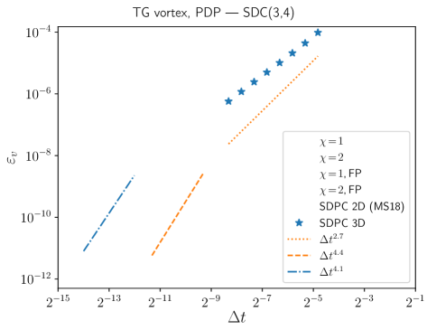
Figure 1. Velocity error of SDC with ${M\!=\!3}$ subintervals and ${K\!=\!4}$ correction sweeps for the Taylor-Green vortex with Dirichlet conditions in the $y$-direction. The choices ${\chi\!=\!1}$ and ${\chi\!=\!2}$ refer to the method based on standard and rotational velocity correction, respectively, and FP indicates the application of the final projection step. SDPC 2D (MS18) represents the two-dimensional results of Minion and Saye [65] and SDPC 3D corresponding three-dimensional results obtained in the present study. The latter extends only down to $\Delta t\approx 2^{-8}$, as the method became increasingly unstable with smaller time steps. (SDPC 2D results courtesy of Michael Minion)

Figure 2 presents the results for cases PPP and PDP obtained with the rotational method for a different number of correction sweeps, ranging from ${K=0}$ to $9$. For PPP the convergence rate grows by one with each correction until the maximum of $2M$ is reached (Fig. 2a). Hence, the method shows the optimal convergence behavior in the periodic case. This can be explained by the lack of a splitting error and was also observed in [65]. In case PDP the imposition of Dirichlet conditions causes an order reduction which manifests in a larger error and a flatter slope for identical $K$ in comparison to PPP (Fig. 2b). Increasing the number of sweeps to ${K=9}$ yields a further error reduction and an improvement of the convergence rate towards the optimal order. This leads to the question on the limiting behavior. For the present example, $8M$ sweeps proved sufficient to approximate the latter. Figure 3 shows the results of a corresponding study with ${M=1,\dots,4}$ subintervals. In contrast to Fig. 2b the limit cases attain nearly constant slopes over a wide range of $\Delta t$. With ${M\!=\!1}$ and $2$ the method achieves the optimal convergence rate of $2M$, whereas ${M\!=\!3}$ exhibits a slight order reduction of about $0.6$. Comparing the latter to ${K\!=\!9}$ in Fig. 2a reveals, however, that the error constant was reduced by nearly two orders of magnitude. With ${M\!=\!4}$ the method is still affected by the instability of the explicit part for the two largest $\Delta t$. After crossing the stability threshold it jumps almost instantly to the spatial error so that no asymptotic slope could be determined. In addition to the standard configuration, i.e. rotational velocity correction with divergence/mass-flux stabilization and final projection, Fig. 3 shows the results for ${M\!=\!3}$ obtained using the standard velocity correction (${\chi\!=\!1}$) with or without stabilization, i.e. ${\tau_{\star}\!=\!0}$ or ${\tau_{\star}\!=\!1}$, respectively, and no final projection. They demonstrate the immense impact of the temporal splitting error and violations of continuity that are caused by the projection method used in the predictor and the corrector. These errors prevent the convergence of the SDC method to the underlying collocation method. However, reducing the time step also diminishes the splitting and continuity errors and may lead an apparent superconvergence as observed in the case ${\chi\!=\!1}$ with ${\tau_{\star}\!=\!0}$. Even the results of rotational method with stabilization and final projection may still differ from the Gauss collocation method. Nevertheless, they meet the expected characteristics except for a mild order reduction. This is a substantial improvement over the SDPC method, which suffers a serious degradation of convergence for ${M>1}$, see [65, Fig. 6.5].

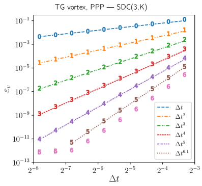
(a) Periodic conditions in $y$-direction.

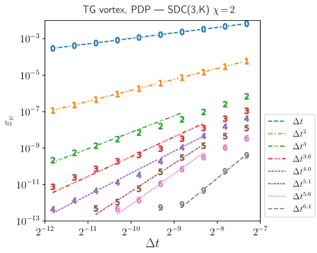
(b) Dirichlet conditions in $y$-direction.

Figure 2. Velocity error for the Taylor-Green vortex with ${M=3}$ subintervals, ${\chi\!=\!2}$ and no final projection. Labels indicate the number of correction sweeps and lines the approximate slope.

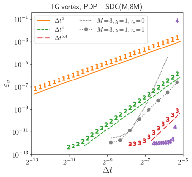
Figure 3. Velocity error of the converged SDC method for the Taylor-Green vortex with Dirichlet conditions in the $y$-direction. Labeled graphs refer to the rotational scheme (${\chi\!=\!2}$) with divergence/mass-flux stabilization ($\tau_{\star}\!=\!1$) and final projection. Digits indicate the number $M$ of subintervals. The dashed lines correspond to the standard scheme (${\chi\!=\!1}$) with or without stabilization ($\tau_{\star}\!=\!0$ or $\tau_{\star}\!=1$) and no final projection.

5.2. Traveling 3D vortex with variable viscosity

5.2.1. Test cases

The suitability for Navier-Stokes problems with variable viscosity is examined on the basis of a manufactured solution proposed by [70]. The exact velocity and pressure are given by

$$v_{x}^{\mathrm{ex}} =\big{[}\sin(2\pi(x+t))+\cos(2\pi(y+t))\big{]}\sin(2\pi(z+t))\,,$$ (91)

$$v_{y}^{\mathrm{ex}} =\big{[}\cos(2\pi(x+t))+\sin(2\pi(y+t))\big{]}\sin(2\pi(z+t))\,,$$ (92)

$$v_{z}^{\mathrm{ex}} =\big{[}\cos(2\pi(x+t))+\cos(2\pi(y+t))\big{]}\cos(2\pi(z+t))\,,$$ (93)

$$p^{\mathrm{ex}} =\sin(2\pi(x+t))\sin(2\pi(y+t))\sin(2\pi(z+t))\,.$$ (94)

Equations (91 – 93) define a periodic vortex array with wave length ${l=1}$ and velocity magnitude ${v^{\mathrm{ex}}_{\max}=2}$, traveling with a phase velocity of 1 in each direction, separately. The exact solution is supplemented with a spatially and temporally varying viscosity of the form ${\nu=\nu_{0}+\nu_{t}(\bm{x},t,\bm{v})}$. Three different scenarios are considered for the fluctuation $\nu_{t}$:

$$\nu_{t}^{(1)}(\bm{x}) =\nu_{1}\sin^{2}(2\pi x)\sin^{2}(2\pi y)\sin^{2}(2\pi z)\,,$$ (95)

$$\nu_{t}^{(2)}(\bm{x},t) =\nu_{1}\sin^{2}(2\pi(x-t))\sin^{2}(2\pi(y-t))\sin^{2}(2\pi(z-t))\,,$$ (96)

$$\nu_{t}^{(3)}(\bm{v}) =\nu_{1}\frac{\bm{v}^{2}}{|\bm{v}^{\mathrm{ex}}|_{\max}^{2}}\,.$$ (97)

Note that the expressions are normalized such that ${\max|\nu_{t}|=\nu_{1}}$ provided that ${\bm{v}=\bm{v}^{\mathrm{ex}}}$. The spatially varying fluctuation $\nu_{t}^{(1)}$ was already given in [70]. Complementing it with a unit phase velocity which is opposed to that of $\bm{v}^{\mathrm{ex}}$ leads to $\nu_{t}^{(2)}$​​. Finally, $\nu_{t}^{(3)}$ depends on the approximate velocity and, thus, renders the viscous term genuinely nonlinear. Based on the above specifications, the RHS of the Navier-Stokes problem is computed as

$$\bm{f}(\bm{x},t)=\partial_{t}\bm{v}^{\mathrm{ex}}+\nabla\cdot\bm{v}^{\mathrm{ex}}\bm{v}^{\mathrm{ex}}-\nabla\cdot\Big{[}\nu(\bm{x},t,\bm{v}^{\mathrm{ex}})\Big{(}\nabla\bm{v}^{\mathrm{ex}}+(\nabla\bm{v}^{\mathrm{ex}})^{\textsc{t}}\Big{)}\Big{]}+\nabla p^{\mathrm{ex}}\,.$$ (98)

Omitting the convection term in (98) yields the RHS of the corresponding Stokes problem.

In all studies reported below time-dependent Dirichlet conditions are imposed such that ${\bm{v}_{\mathrm{b}}=\bm{v}^{\mathrm{ex}}}$ on $\partial\Omega$.

5.2.2. Influence of the base time-integration scheme

To investigate the role of the parameter $\chi$ and the final projection in the predictor and corrector, a preliminary study was conducted for a solution-dependent viscosity $\nu^{(3)}$ with coefficients ${\nu_{0}=\nu_{1}=10^{-2}}$. This choice corresponds to Reynolds number of ${\mathit{Re}={lv_{\max}}/{\nu_{\mathrm{ref}}}\approx 133}$, where ${\nu_{\mathrm{ref}}=\nu_{0}+\frac{1}{2}\nu_{1}}$. The numerical tests were computed in the domain ${\Omega=[-\nicefrac{{1}}{{2}},\nicefrac{{1}}{{2}}]^{3}}$ for ${t\leq 0.25}$. Spatial discretization is based on a uniform mesh comprising $2^{3}$ cubic elements of degree ${P=16}$. For time integration the SDC method was applied with ${M=6}$ and ${K=11}$ correction sweeps. Figure 4 shows the resulting velocity error for different predictor/corrector variants. As in case of the Taylor-Green vortex, the variants with FP achieve the best results and virtually coincide regardless of the choice for $\chi$. They reach a convergence rate of approximately 7.5, which corresponds to a reduction of 4.5 or 37.5 percent of the expected order of 12. The standard scheme (${\chi=1}$) with no FP attains almost the same accuracy, whereas the rotational scheme (${\chi=2}$) converges at a rate of only about 4.8. This contradicts the results obtained with the Taylor-Green vortex, for which the rotational scheme surpassed the standard one. These observations indicate that the final projection eliminates a substantial part of the splitting error, while the choice of $\chi$ is of minor importance. Based on these observations, all of the following studies use the rotational scheme with FP.

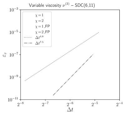
Figure 4. Velocity error of SDC with ${M=6}$ subintervals and ${K=11}$ correction sweeps for the traveling 3D vortex with solution-dependent viscosity. The choices ${\chi\!=\!1}$ and ${\chi\!=\!2}$ refer to the method based on standard and rotational velocity correction, respectively, and FP indicates the application of the final projection step.

5.2.3. Temporal convergence

Three different scenarios were chosen for assessing the robustness of the SDC method against variable viscosity: 1) spatially varying, ${\nu(\bm{x})=\nu^{(1)}}$, 2) spatiotemporally varying, ${\nu(\bm{x},t)=\nu^{(2)}}$, and 3) solution-dependent, ${\nu(\bm{v})=\nu^{(3)}}$, with coefficients ${\nu_{0}=\nu_{1}=10^{-2}}$. Additionally, the case with constant ${\nu=0.015}$ is considered for reference. The computational domain, spatial discretization and final time are identical to the previous study. Figure 5 shows the velocity error obtained with ${M=6}$ subintervals and a different number of correction sweeps, ranging from ${K=0}$ up to $30$. All investigated scenarios exhibit a similar behavior and achieve convergence rates comparable to the reference case. Using 30 corrections yields a rate of 12, which equals the theoretical order of the underlying collocation method. Runs with a lower number of sweeps suffer an order reduction. The extent of this reduction is similar for all scenarios, which indicates that the presence of a variable viscosity is not the primary cause. As in the previous test case it is more likely to be caused by the boundary treatment and the splitting error of the underlying projection method. It is further noted that Fig. 5b and 5c lack the errors for the two largest time steps with ${K=30}$. This is because $\Delta t$ exceeds the long term stability threshold, which is considered in more detail below.

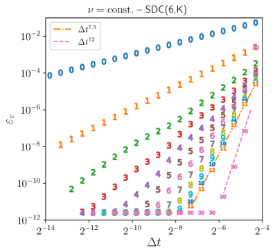
(a) Constant viscosity.

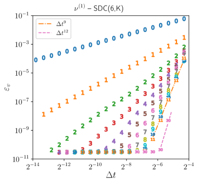
(b) Spatially varying viscosity.

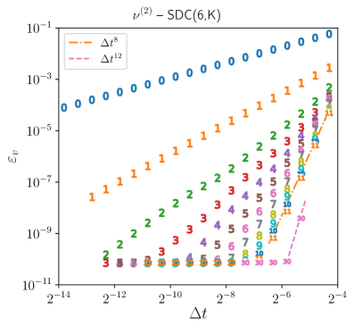
(c) Spatiotemporally varying viscosity.

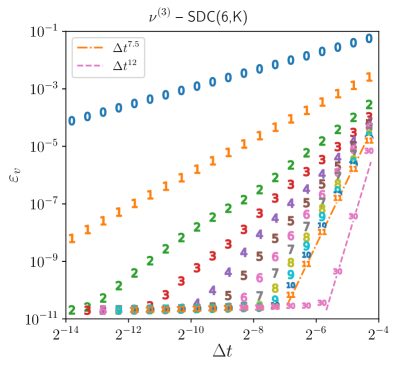
(d) Solution-dependent viscosity.

Figure 5. Velocity error for different viscosity scenarios using SDC with ${M=6}$ subintervals. Labels indicate the number of correction sweeps and lines the approximate slope.

As discussed in Sec. 3.2.3, the SDC method does not provide the discrete pressure. It can be computed, however, by solving the discrete version of the consistent pressure equation (44). This yields the pressure with an accuracy comparable to that of velocity, see, e.g., Fig. 6a for the case of solution-dependent viscosity. Figure 6 depicts the corresponding divergence error. Except for larger time steps with ${K=1}$ it shows roughly the same behavior as the velocity and pressure errors. Additional studies revealed that an even stronger divergence penalization fails to reduce $\varepsilon_{\mathrm{div}}$ significantly. This observation is somewhat surprising. It can be explained with the splitting error in the final projection step, which incurs a violation of the tangential velocity boundary conditions and causes a growth of divergence near the edges of the computational domain.

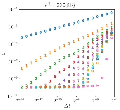
(a) Pressure error.

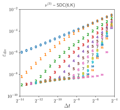
(b) Divergence.

Figure 6. Pressure and divergence errors obtained for the case of solution-dependent viscosity.

5.2.4. Convergence towards the collocation solution

To assess the limiting behavior for variable viscosity, the SDC method was applied with ${M=1,\dots,6}$ subintervals and ${K\!=\!8M}$ correction sweeps. Figure 7 shows the most challenging case with a solution-dependent viscosity. Similarly to the Taylor-Green example, regular convergence with the expected rate of $2M$ is observed for ${M\!=\!1}$ and $2$, whereas ${M\!=\!3}$ exhibits a slight reduction of half an order. For time steps ${\Delta t>2^{-5}}$ the method is affected by the instability of the explicit part with $M\geq 3$. Additionally, the splitting error may still be significant here. The cumulative effect of both factors could explain the superconvergence observed for $M\geq 4$.

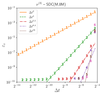
Figure 7. Velocity error of the converged SDC method for the case of solution-dependent viscosity. Labels indicate the number $M$ of subintervals.

5.2.5. Stability

The stability of the SDC method was investigated for the limiting cases of convection-dominated flow and Stokes flow. For this study the domain ${\Omega=[-\nicefrac{{1}}{{2}},\nicefrac{{1}}{{2}}]^{3}}$ was discretized in three ways: 1) $6^{3}$ elements of degree ${P\!=\!6}$, 2) $3^{3}$ elements of degree 11 and 3) $2^{3}$ elements of degree 16. The numerical tests were run until reaching the final time ${T=10}$, which corresponds to 10 convective units in terms of the phase velocity. A test was considered unstable when exceeding a velocity magnitude of ${v^{\mathrm{ex}}_{\max}/2}$ or detecting a NaN in the numerical solution. Based on this criterion the time step was adapted via bisection until a reaching sufficiently accurate approximation of the critical time step $\Delta t^{\ast}$.

In the convection-dominated case the viscosity $\nu^{(1)}$ is adopted with ${\nu_{0}=\nu_{1}=10^{-3}}$. This corresponds to a Reynolds number of approximately 1333, based on $v^{\mathrm{ex}}_{\max}$ and ${\nu_{\mathrm{ref}}=\nu_{0}+\frac{1}{2}\nu_{1}}$. The resulting convective stability threshold is converted into dimensionless form by introducing the critical Courant-Friedrichs-Lewy (CFL) number

$$\mathit{CFL}^{\ast}=\frac{\Delta t^{\ast}v_{\max}}{\delta}\,,$$ (99)

where $\delta$ is a length scale characterizing the mesh spacing. For high-order element methods different length scales have been proposed, in particular, ${\delta_{1}=h/(P+1)}$ and ${\delta_{2}=h/P^{2}}$, see e.g. [39, 53]. The corresponding CFL numbers are denoted as $\mathit{CFL}^{\ast}_{1}$ and $\mathit{CFL}^{\ast}_{2}$, respectively. Alternatively, the length scale can be defined as the inverse maximum modulus of the eigenvalues of the one-dimensional element convection operator, i.e., ${\delta_{\lambda}=|\lambda|_{\max}^{-1}}$. In the present case, the eigenvalues result from the GLL collocation differentiation operator of degree $P$ combined with one-sided Dirichlet conditions. For details see Canuto et al. [17, Sec. 7.3.3]. The resulting CFL number is denoted as $\mathit{CFL}^{\ast}_{\lambda}$. Tabular 1 compiles the critical CFL numbers determined in this study. Note that the first three lines correspond to the case with only one subinterval. Starting with the split semi-implicit Euler method (${K\!=\!0}$), the admissible time step grows by factor of 3 with one correction and even a factor of $5.3$ with two. Elevating the number of subintervals and, proportionally, the number correction sweeps yields a further increase of the stability threshold. A comparison of the stability limits for equal $M$ further reveals a strong dependence of $\mathit{CFL}^{\ast}_{1}$ and $\mathit{CFL}^{\ast}_{2}$ on $P$, whereas $\mathit{CFL}^{\ast}_{\lambda}$ is virtually independent of the polynomial degree. Figure 8 confirms this observation and, moreover, illustrates that the stability threshold grows linearly when increasing the number of subintervals. This behavior was expected, since the predictor and the corrector perform substeps with the size scaling as ${\Delta t/M}$. Given the influence of the flow configuration, the Reynolds number, the stability and dissipativity of spatial discretization and the termination criterium, these results cannot be compared directly to other studies. Despite this limitation, the $\mathit{CFL}^{\ast}_{2}$ observed for the second-order SDC method (${M\!=\!1}$, ${K\!=\!2}$) reside in the same range as those reported by Fehn et al. [34], who used a similar space discretization combined with a semi-implicit projection method of order 2.

It should be noted that the SDC method based on IMEX Euler is potentially unstable in the purely convective case. For example, according to [67, Fig. 4.4] the stability region includes no part of the imaginary axis for $K=M$ with $M=5$ and $6$. Moreover, the convection term of the flow problem may give rise to nonlinear instability. The arising instabilities often grow with further correction sweeps so that no convergence to the corresponding Gauß method can be achieved. Both effects, marginal linear stability and nonlinearity, prevent the deduction of a reliable stability criterion for convection, which leaves an inconvenience for the application to high Reynolds number flows.

Table 1. Critical CFL numbers for ${\mathit{Re}\approx 1333}$ and SDC with a different number of subintervals $M$ and corrections sweeps $K$.

			$P=6$				$P=11$				$P=16$
$M$	$K$		$\mathit{CFL}^{\ast}_{1}$	$\mathit{CFL}^{\ast}_{2}$	$\mathit{CFL}^{\ast}_{\lambda}$		$\mathit{CFL}^{\ast}_{1}$	$\mathit{CFL}^{\ast}_{2}$	$\mathit{CFL}^{\ast}_{\lambda}$		$\mathit{CFL}^{\ast}_{1}$	$\mathit{CFL}^{\ast}_{2}$	$\mathit{CFL}^{\ast}_{\lambda}$
$1$	$0$		$.174$	$.895$	$.222$		$.142$	$1.43$	$.277$		$.118$	$1.78$	$.317$
$1$	$1$		$.522$	$2.68$	$.667$		$.368$	$3.72$	$.720$		$.275$	$4.14$	$.737$
$1$	$2$		$.922$	$4.74$	$1.18$		$.639$	$6.45$	$1.25$		$.476$	$7.17$	$1.28$
$2$	$4$		$1.16$	$5.97$	$1.48$		$.781$	$7.87$	$1.53$		$.551$	$8.29$	$1.48$
$3$	$6$		$1.41$	$7.25$	$1.80$		$.925$	$9.32$	$1.81$		$.673$	$10.1$	$1.80$
$4$	$8$		$1.75$	$9.02$	$2.24$		$1.14$	$11.6$	$2.24$		$.818$	$12.3$	$2.19$
$5$	$10$		$2.09$	$10.7$	$2.67$		$1.37$	$13.8$	$2.68$		$.966$	$14.5$	$2.59$
$6$	$12$		$2.38$	$12.3$	$3.04$		$1.54$	$15.6$	$3.02$		$1.09$	$16.4$	$2.91$
$7$	$14$		$2.64$	$13.6$	$3.38$		$1.71$	$17.2$	$3.34$		$1.21$	$18.2$	$3.25$
$8$	$16$		$2.92$	$15.0$	$3.74$		$1.89$	$19.1$	$3.70$		$1.34$	$20.1$	$3.58$

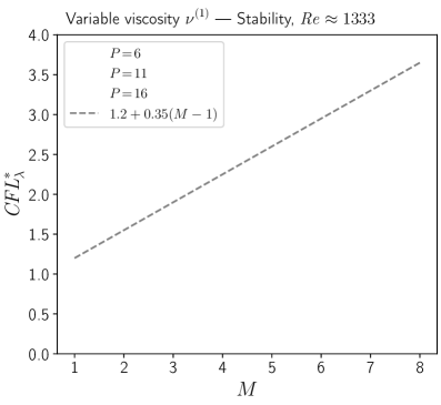
Figure 8. Critical CFL number for a varying number of subintervals $M$ and ${K=2M}$ correction sweeps.

A similar study was conducted for the Stokes flow with solution-dependent viscosity $\nu^{(3)}$ featuring ${\nu_{0}=\nu_{1}=1}$. Notwithstanding the semi-implicit treatment of the viscous term all test runs remained stable up to the maximal time step size of ${\Delta t=5}$, which is about $10^{4}$ times the diffusive fluctuation time scale ${\tau_{\mathrm{d}}=\nicefrac{{h^{2}}}{{\nu_{1}P^{4}}}}$. This allows the conclusion that the semi-implicit approach does not affect the stability of the SDC method for viscosity fluctuations up to at least 50 percent.

5.2.6. Spatial convergence

The final study serves for examining the spatial convergence with variable viscosity. It is based on the on the highly-nonlinear, solution-dependent viscosity $\nu^{(3)}$ with coefficients ${\nu_{0}=\nu_{1}=10^{-2}}$. The numerical tests were computed in the domain ${\Omega=[-2,2]^{3}}$ for polynomial degrees up to ${P=16}$. Starting from one, the number of elements per direction was gradually increased to at least 8. Time integration was performed using the SDC method with ${M=6}$ and ${K=11}$ until reaching ${T=0.25}$. The time step size was confined to ${\Delta t=2^{-8}}$ such that the temporal discretization error is negligible. Figure 9 shows the velocity error for polynomial degrees ${P=6}$, $11$ and $16$. In all three cases the method converges approximately with $h^{P+1}$. This result is surprising, since the viscous terms are integrated with just ${P+1}$ GLL points, for which only order $P$ is expected [63]. Possibly, the higher convergence rate is promoted by the construction of the test case. Clarifying this issue requires an in-depth investigation, which is beyond the scope of the present work.

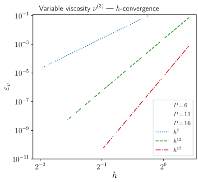
Figure 9. Spatial convergence with solution-dependent variable viscosity.

6. Conclusions

This paper presents a high-order, semi-implicit time-integration strategy for incompressible Navier-Stokes problems with variable viscosity based on the spectral deferred correction (SDC) method. Combining SDC with the discontinuous Galerkin spectral-element method for spatial discretization yields a powerful approach for targeting arbitrary order in space and time.

The key ingredients of the method, the predictor and the corrector, are derived from a first-order velocity-correction method, which is augmented by an additional projection step to remove divergence errors caused by variable viscosity. In contrast to the SDPC method of Minion and Saye [65], the pressure occurs only as an auxiliary variable in the substeps and needs not to be stored. Furthermore, mixed-order (${P/P\!-\!1}$) polynomial approximations are used for inf-sup stability and combined with divergence/mass-flux stabilization for pressure robustness [3].

The performance of the SDC method was assessed at the example of a Taylor-Green (TG) vortex and a manufactured 3D vortex array, both traveling with a prescribed phase velocity. The latter involves a variable viscosity $\nu$ that can be chosen to depend on space, space and time, or on the velocity $\bm{v}$. For the TG vortex with constant viscosity and periodic boundaries, each correction sweep lifted the order by 1 as expected. Imposing time-dependent Dirichlet boundary conditions, however, led to a more irregular convergence behavior accompanied by an order reduction. For a fixed number of corrections, convergence starts at a lower rate and at a higher error level than in the periodic case. With decreasing size of the time step $\Delta t$ it accelerates and can even reach a rate higher than the theoretical order. A closer inspection revealed that this behavior is most likely a manifestation of the splitting error of the time integration scheme adopted for the corrector. Using the rotational velocity correction augmented by divergence/mass-flux stabilization and a final projection step allowed to minimize this error and lowered the resulting order reduction to approximately $0.2$ per sweep. The investigation showed that the splitting error also affects the limit case which arises after a sufficient number of corrections. While the optimized corrector based on the rotational velocity-correction exhibited a nearly ideal convergence behavior with only a slight order reduction, other variants suffered a severe degradation. Moreover, these observations offer an explanation for the results of Minion and Saye [65] who achieved only about half the expected order in the limit case. Thus, it is not surprising that the proposed SDC method clearly outperforms SDPC except for the periodic case, for which the splitting error disappears. Finally, the new method proved robust and almost equally efficient with variable viscosity, even in the nonlinear case, where the latter depends on the solution itself. This case also served as a test bed for exploring the temporal stability. Considering a convection-dominated regime, the critical CFL number grows linearly with the number of SDC subintervals and virtually coincides for different polynomial degrees, when choosing the length scale based on eigenvalues of the DG differentiation operator. In the Stokes case with variable viscosity, the method remains stable for steps up to at lest 4 orders of magnitude above the viscous time scale $\nicefrac{{h^{2}}}{{P^{4}\nu}}$, where $h$ is the element size and $P$ the polynomial degree of the discrete velocity.

The present study suggests that a further improvement is possible by eliminating the residual splitting error. This could be achieved by performing a coupled iteration within each Euler step or using a higher order method for constructing the corrector. Of course, the ultimate goal is to render the SDC method competitive to common approaches such as multistep and Runge-Kutta methods. This may require further measures. For example, a higher-order time-integration method can be harnessed as the predictor to gain a more accurate initial approximation and conditional stability in the convective limit [59]. Using uniform instead of Gaussian quadrature points in time, such methods may also accelerate the corrector [27]. Alternatively, the number of iterations could be reduced by adopting suitable preconditioners like the LU-decomposition proposed in [87] or space-time multilevel strategies such as MLSDC [78] and their parallel descendants [69, 77]. Utilizing these techniques for designing faster flow solvers is the topic of ongoing research and will be addressed in future papers.

References

- Ahmed et al. [2017] N. Ahmed, S. Becher, and G. Matthies. Higher-order discontinuous Galerkin time stepping and local projection stabilization techniques for the transient Stokes problem. Computer Methods in Applied Mechanics and Engineering, 313:28–52, jan 2017. doi: 10.1016/j.cma.2016.09.026.
- Ainsworth and Wajid [2009] M. Ainsworth and H. A. Wajid. Dispersive and dissipative behavior of the spectral element method. SIAM Journal on Numerical Analysis, 47(5):3910–3937, jan 2009. doi: 10.1137/080724976.
- Akbas et al. [2018] M. Akbas, A. Linke, L. G. Rebholz, and P. W. Schroeder. The analogue of grad-div stabilization in DG methods for incompressible flows: Limiting behavior and extension to tensor-product meshes. Computer Methods in Applied Mechanics and Engineering, 341:917–938, nov 2018. doi: 10.1016/j.cma.2018.07.019.
- Almgren et al. [2013] A. S. Almgren, A. J. Aspden, J. B. Bell, and M. L. Minion. On the use of higher-order projection methods for incompressible turbulent flow. SIAM Journal on Scientific Computing, 35(1):B25–B42, jan 2013. doi: 10.1137/110829386.
- Alonso-Mallo [2002] I. Alonso-Mallo. Runge-Kutta methods without order reduction for linear initial boundary value problems. Numerische Mathematik, 91(4):577–603, jun 2002. doi: 10.1007/s002110100332.
- Alonso-Mallo et al. [2005] I. Alonso-Mallo, B. Cano, and M. Moreta. Order reduction and how to avoid it when explicit Runge–Kutta–Nyström methods are used to solve linear partial differential equations. Journal of Computational and Applied Mathematics, 176(2):293–318, Apr 2005. ISSN 0377-0427. doi: 10.1016/j.cam.2004.07.021. URL http://dx.doi.org/10.1016/j.cam.2004.07.021.
- Arnold et al. [2001] D. N. Arnold, F. Brezzi, B. Cockburn, and L. D. Marini. Unified analysis of discontinuous Galerkin methods for elliptic problems. SIAM Journal on Numerical Analysis, 39(5):1749–1779, 2001.
- Ascher et al. [1997] U. M. Ascher, S. J. Ruuth, and R. J. Spiteri. Implicit-explicit Runge-Kutta methods for time-dependent partial differential equations. Applied Numerical Mathematics, 25(2-3):151–167, Nov 1997. ISSN 0168-9274. doi: 10.1016/s0168-9274(97)00056-1. URL http://dx.doi.org/10.1016/S0168-9274(97)00056-1.
- Bassi et al. [2015] F. Bassi, L. Botti, A. Colombo, A. Ghidoni, and F. Massa. Linearly implicit Rosenbrock-type Runge–Kutta schemes applied to the discontinuous Galerkin solution of compressible and incompressible unsteady flows. Computers & Fluids, 118:305–320, Sep 2015. ISSN 0045-7930. doi: 10.1016/j.compfluid.2015.06.007. URL http://dx.doi.org/10.1016/j.compfluid.2015.06.007.
- Beck et al. [2014] A. D. Beck, T. Bolemann, D. Flad, H. Frank, G. J. Gassner, F. Hindenlang, and C.-D. Munz. High-order discontinuous Galerkin spectral element methods for transitional and turbulent flow simulations. International Journal for Numerical Methods in Fluids, 76(8):522–548, aug 2014. doi: 10.1002/fld.3943.
- Boffi et al. [2013] D. Boffi, F. Brezzi, and M. Fortin. Mixed finite element methods and applications. Springer Series in Computational Mathematics, 2013. ISSN 0179-3632. doi: 10.1007/978-3-642-36519-5. URL http://dx.doi.org/10.1007/978-3-642-36519-5.
- Bolten et al. [2017] M. Bolten, D. Moser, and R. Speck. A multigrid perspective on the parallel full approximation scheme in space and time. Numerical Linear Algebra with Applications, 24(6):e2110, Jun 2017. ISSN 1070-5325. doi: 10.1002/nla.2110. URL http://dx.doi.org/10.1002/nla.2110.
- Boscarino et al. [2016] S. Boscarino, F. Filbet, and G. Russo. High order semi-implicit schemes for time dependent partial differential equations. Journal of Scientific Computing, 68(3):975–1001, jan 2016. doi: 10.1007/s10915-016-0168-y.
- Burrage and Petzold [1990] K. Burrage and L. Petzold. On order reduction for Runge–Kutta methods applied to differential/algebraic systems and to stiff systems of ODEs. SIAM Journal on Numerical Analysis, 27(2):447–456, Apr 1990. ISSN 1095-7170. doi: 10.1137/0727027. URL http://dx.doi.org/10.1137/0727027.
- Buscariolo et al. [2019] F. F. Buscariolo, J. Hoessler, D. Moxey, A. Jassim, K. Gouder, J. Basley, Y. Murai, G. R. S. Assi, and S. J. Sherwin. Spectral/hp element simulation of flow past a Formula One front wing: validation against experiments, 2019.
- Canuto et al. [2007] C. Canuto, M. Y. Hussaini, A. Quarteroni, and T. A. Zang. Spectral Methods. Evolution to Complex Geometries and Applications to Fluid Dynamics. Springer-Verlag GmbH, 2007. ISBN 3540307273. URL https://www.ebook.de/de/product/5226601/claudio_canuto_m_yousuff_hussaini_alfio_quarteroni_thomas_a_zang_spectral_methods.html.
- Canuto et al. [2011] C. Canuto, M. Y. Hussaini, A. Quarteroni, and T. A. Zang. Spectral Methods. Fundamentals in Single Domains. Springer Berlin Heidelberg, 2011. ISBN 3540307257. URL https://www.ebook.de/de/product/5194670/claudio_canuto_m_yousuff_hussaini_alfio_quarteroni_thomas_a_zang_spectral_methods.html.
- Carpenter et al. [1995] M. H. Carpenter, D. Gottlieb, S. Abarbanel, and W.-S. Don. The theoretical accuracy of Runge–Kutta time discretizations for the initial boundary value problem: A study of the boundary error. SIAM Journal on Scientific Computing, 16(6):1241–1252, Nov 1995. ISSN 1095-7197. doi: 10.1137/0916072. URL http://dx.doi.org/10.1137/0916072.
- Causley and Seal [2019] M. Causley and D. Seal. On the convergence of spectral deferred correction methods. Communications in Applied Mathematics and Computational Science, 14(1):33–64, Feb 2019. ISSN 1559-3940. doi: 10.2140/camcos.2019.14.33. URL http://dx.doi.org/10.2140/camcos.2019.14.33.
- Cavaglieri and Bewley [2015] D. Cavaglieri and T. Bewley. Low-storage implicit/explicit Runge-Kutta schemes for the simulation of stiff high-dimensional ODE systems. Journal of Computational Physics, 286:172–193, apr 2015. doi: 10.1016/j.jcp.2015.01.031.
- Chan et al. [2017] J. Chan, R. J. Hewett, and T. Warburton. Weight-adjusted discontinuous Galerkin methods: Wave propagation in heterogeneous media. SIAM Journal on Scientific Computing, 39(6):A2935–A2961, jan 2017. doi: 10.1137/16m1089186.
- Chen and Liu [2013] J. Chen and Q. H. Liu. Discontinuous Galerkin time-domain methods for multiscale electromagnetic simulations: A review. Proceedings of the IEEE, 101(2):242–254, feb 2013. doi: 10.1109/jproc.2012.2219031.
- Chorin [1968] A. J. Chorin. Numerical solution of the Navier-Stokes equations. Mathematics of Computation, 22(104):745–745, 1968. doi: 10.1090/s0025-5718-1968-0242392-2.
- Christlieb et al. [2009a] A. Christlieb, B. Ong, and J.-M. Qiu. Comments on high-order integrators embedded within integral deferred correction methods. Communications in Applied Mathematics and Computational Science, 4(1):27–56, jun 2009a. doi: 10.2140/camcos.2009.4.27.
- Christlieb et al. [2009b] A. Christlieb, B. Ong, and J.-M. Qiu. Integral deferred correction methods constructed with high order Runge–Kutta integrators. Mathematics of Computation, 79(270):761–783, Sep 2009b. ISSN 0025-5718. doi: 10.1090/s0025-5718-09-02276-5. URL http://dx.doi.org/10.1090/S0025-5718-09-02276-5.
- Christlieb et al. [2011] A. Christlieb, M. Morton, B. Ong, and J.-M. Qiu. Semi-implicit integral deferred correction constructed with additive Runge–Kutta methods. Communications in Mathematical Sciences, 9(3):879–902, 2011. ISSN 1945-0796. doi: 10.4310/cms.2011.v9.n3.a10. URL http://dx.doi.org/10.4310/CMS.2011.v9.n3.a10.
- Christlieb et al. [2015] A. J. Christlieb, Y. Liu, and Z. Xu. High order operator splitting methods based on an integral deferred correction framework. Journal of Computational Physics, 294:224–242, Aug 2015. ISSN 0021-9991. doi: 10.1016/j.jcp.2015.03.032. URL http://dx.doi.org/10.1016/j.jcp.2015.03.032.
- Constantinescu and Sandu [2010] E. M. Constantinescu and A. Sandu. Extrapolated implicit-explicit time stepping. SIAM Journal on Scientific Computing, 31(6):4452–4477, Jan 2010. ISSN 1095-7197. doi: 10.1137/080732833. URL http://dx.doi.org/10.1137/080732833.
- Delcourte and Glinsky [2015] S. Delcourte and N. Glinsky. Analysis of a high-order space and time discontinuous Galerkin method for elastodynamic equations. application to 3d wave propagation. ESAIM: Mathematical Modelling and Numerical Analysis, 49(4):1085–1126, jun 2015. doi: 10.1051/m2an/2015001.
- Deteix and Yakoubi [2018] J. Deteix and D. Yakoubi. Improving the pressure accuracy in a projection scheme for incompressible fluids with variable viscosity. Appl. Math. Lett., 79:111–117, 2018.
- Deville et al. [2002] M. O. Deville, P. F. Fischer, and E. H. Mund. High-Order Methods for Incompressible Fluid Flow. Cambridge University Press, 2002. ISBN 9780521453097. doi: 10.1017/cbo9780511546792. URL http://dx.doi.org/10.1017/CBO9780511546792.
- Dutt et al. [2000] A. Dutt, L. Greengard, and V. Rokhlin. Spectral deferred correction methods for ordinary differential equations. Bit Numerical Mathematics, 40(2):241–266, 2000. doi: 10.1023/a:1022338906936.
- Fai et al. [2014] T. G. Fai, B. E. Griffith, Y. Mori, and C. S. Peskin. Immersed boundary method for variable viscosity and variable density problems using fast constant-coefficient linear solvers ii: Theory. SIAM Journal on Scientific Computing, 36(3):B589–B621, Jan 2014. ISSN 1095-7197. doi: 10.1137/12090304x. URL http://dx.doi.org/10.1137/12090304X.
- Fehn et al. [2017] N. Fehn, W. A. Wall, and M. Kronbichler. On the stability of projection methods for the incompressible Navier-Stokes equations based on high-order discontinuous Galerkin discretizations. Journal of Computational Physics, 351:392–421, dec 2017. doi: 10.1016/j.jcp.2017.09.031.
- Fehn et al. [2019] N. Fehn, M. Kronbichler, C. Lehrenfeld, G. Lube, and P. W. Schroeder. High-order DG solvers for underresolved turbulent incompressible flows: A comparison of and methods. International Journal for Numerical Methods in Fluids, 91(11):533–556, aug 2019. doi: 10.1002/fld.4763.
- Ferrer et al. [2014] E. Ferrer, D. Moxey, R. H. J. Willden, and S. J. Sherwin. Stability of projection methods for incompressible flows using high order pressure-velocity pairs of same degree: Continuous and discontinuous Galerkin formulations. Communications in Computational Physics, 16(3):817–840, Sep 2014. ISSN 1991-7120. doi: 10.4208/cicp.290114.170414a. URL http://dx.doi.org/10.4208/cicp.290114.170414a.
- Friedrich et al. [2019] L. Friedrich, G. Schnücke, A. R. Winters, D. C. D. R. Fernández, G. J. Gassner, and M. H. Carpenter. Entropy stable space–time discontinuous Galerkin schemes with summation-by-parts property for hyperbolic conservation laws. Journal of Scientific Computing, 80(1):175–222, Mar 2019. ISSN 1573-7691. doi: 10.1007/s10915-019-00933-2. URL http://dx.doi.org/10.1007/s10915-019-00933-2.
- Gardner et al. [2018] D. J. Gardner, J. E. Guerra, F. P. Hamon, D. R. Reynolds, P. A. Ullrich, and C. S. Woodward. Implicit–explicit (IMEX) Runge–Kutta methods for non-hydrostatic atmospheric models. Geoscientific Model Development, 11(4):1497–1515, Apr 2018. ISSN 1991-9603. doi: 10.5194/gmd-11-1497-2018. URL http://dx.doi.org/10.5194/gmd-11-1497-2018.
- Gassner and Kopriva [2011] G. Gassner and D. A. Kopriva. A comparison of the dispersion and dissipation errors of Gauss and Gauss–Lobatto discontinuous Galerkin spectral element methods. SIAM Journal on Scientific Computing, 33(5):2560–2579, jan 2011. doi: 10.1137/100807211.
- Glowinski [2003] R. Glowinski. Finite element methods for incompressible viscous flow. In Handbook of Numerical Analysis, pages 3–1176. Elsevier, 2003. doi: 10.1016/s1570-8659(03)09003-3.
- Gottlieb et al. [2001] S. Gottlieb, C.-W. Shu, and E. Tadmor. Strong stability-preserving high-order time discretization methods. SIAM Review, 43(1):89–112, jan 2001. doi: 10.1137/s003614450036757x.
- Guermond et al. [2006] J. Guermond, P. Minev, and J. Shen. An overview of projection methods for incompressible flows. Computer Methods in Applied Mechanics and Engineering, 195(44-47):6011–6045, sep 2006. doi: 10.1016/j.cma.2005.10.010.
- Guermond and Shen [2003] J. L. Guermond and J. Shen. Velocity-correction projection methods for incompressible flows. SIAM Journal on Numerical Analysis, 41(1):112–134, jan 2003. doi: 10.1137/s0036142901395400.
- Hairer and Wanner [1996] E. Hairer and G. Wanner. Solving Ordinary Differential Equations II. Springer Berlin Heidelberg, 1996. doi: 10.1007/978-3-642-05221-7.
- Hairer et al. [1993] E. Hairer, S. P. Nørsett, and G. Wanner. Solving Ordinary Differential Equations I. Springer Berlin Heidelberg, 1993. doi: 10.1007/978-3-540-78862-1.
- Hesthaven and Warburton [2008] J. S. Hesthaven and T. Warburton. Nodal Discontinuous Galerkin Methods. Springer, 2008.
- Higueras et al. [2014] I. Higueras, N. Happenhofer, O. Koch, and F. Kupka. Optimized strong stability preserving IMEX Runge–Kutta methods. Journal of Computational and Applied Mathematics, 272:116–140, Dec 2014. ISSN 0377-0427. doi: 10.1016/j.cam.2014.05.011. URL http://dx.doi.org/10.1016/j.cam.2014.05.011.
- Huang et al. [2006] J. Huang, J. Jia, and M. Minion. Accelerating the convergence of spectral deferred correction methods. Journal of Computational Physics, 214(2):633–656, may 2006. doi: 10.1016/j.jcp.2005.10.004.
- Huismann et al. [2020] I. Huismann, J. Stiller, and J. Fröhlich. Efficient high-order spectral element discretizations for building block operators of CFD. Computers & Fluids, 197:104386, 2020. doi: 10.1016/j.compfluid.2019.104386.
- John [2016] V. John. Finite element methods for incompressible flow problems. Springer Series in Computational Mathematics, 2016. ISSN 2198-3712. doi: 10.1007/978-3-319-45750-5. URL http://dx.doi.org/10.1007/978-3-319-45750-5.
- John et al. [2006] V. John, G. Matthies, and J. Rang. A comparison of time-discretization/linearization approaches for the incompressible Navier–Stokes equations. Computer Methods in Applied Mechanics and Engineering, 195(44-47):5995–6010, Sep 2006. ISSN 0045-7825. doi: 10.1016/j.cma.2005.10.007. URL http://dx.doi.org/10.1016/j.cma.2005.10.007.
- Joshi et al. [2016] S. M. Joshi, P. J. Diamessis, D. T. Steinmoeller, M. Stastna, and G. N. Thomsen. A post-processing technique for stabilizing the discontinuous pressure projection operator in marginally-resolved incompressible inviscid flow. Computers & Fluids, 139:120–129, nov 2016. doi: 10.1016/j.compfluid.2016.04.021.
- Karniadakis and Sherwin [2005] G. Karniadakis and S. Sherwin. Spectral/hp Element Methods for Computational Fluid Dynamics. Oxford University Press, jun 2005. doi: 10.1093/acprof:oso/9780198528692.001.0001.
- Karniadakis et al. [1991] G. E. Karniadakis, M. Israeli, and S. A. Orszag. High-order splitting methods for the incompressible Navier-Stokes equations. Journal of Computational Physics, 97(2):414–443, dec 1991. doi: 10.1016/0021-9991(91)90007-8.
- Kennedy and Carpenter [2003] C. A. Kennedy and M. H. Carpenter. Additive Runge-Kutta schemes for convection-diffusion-reaction equations. Applied Numerical Mathematics, 44(1-2):139–181, jan 2003. doi: 10.1016/s0168-9274(02)00138-1.
- Klein et al. [2015] B. Klein, F. Kummer, M. Keil, and M. Oberlack. An extension of the SIMPLE based discontinuous Galerkin solver to unsteady incompressible flows. International Journal for Numerical Methods in Fluids, 77(10):571–589, jan 2015. doi: 10.1002/fld.3994.
- Krank et al. [2017] B. Krank, N. Fehn, W. A. Wall, and M. Kronbichler. A high-order semi-explicit discontinuous Galerkin solver for 3D incompressible flow with application to DNS and LES of turbulent channel flow. Journal of Computational Physics, 348:634–659, nov 2017. doi: 10.1016/j.jcp.2017.07.039.
- Kress and Gustafsson [2002] W. Kress and B. Gustafsson. Deferred correction methods for initial boundary value problems. Journal of Scientific Computing, 17(1/4):241–251, 2002. ISSN 0885-7474. doi: 10.1023/a:1015113017248. URL http://dx.doi.org/10.1023/A:1015113017248.
- Layton and Minion [2007] A. Layton and M. Minion. Implications of the choice of predictors for semi-implicit picard integral deferred correction methods. Communications in Applied Mathematics and Computational Science, 2(1):1–34, Aug 2007. ISSN 1559-3940. doi: 10.2140/camcos.2007.2.1. URL http://dx.doi.org/10.2140/camcos.2007.2.1.
- Layton [2008] A. T. Layton. On the choice of correctors for semi-implicit picard deferred correction methods. Applied Numerical Mathematics, 58(6):845–858, Jun 2008. ISSN 0168-9274. doi: 10.1016/j.apnum.2007.03.003. URL http://dx.doi.org/10.1016/j.apnum.2007.03.003.
- Layton and Minion [2005] A. T. Layton and M. L. Minion. Implications of the choice of quadrature nodes for picard integral deferred corrections methods for ordinary differential equations. BIT Numerical Mathematics, 45(2):341–373, Jun 2005. ISSN 1572-9125. doi: 10.1007/s10543-005-0016-1. URL http://dx.doi.org/10.1007/s10543-005-0016-1.
- Leriche et al. [2006] E. Leriche, E. Perchat, G. Labrosse, and M. O. Deville. Numerical evaluation of the accuracy and stability properties of high-order direct Stokes solvers with or without temporal splitting. Journal of Scientific Computing, 26(1):25–43, Jan 2006. ISSN 1573-7691. doi: 10.1007/s10915-004-4798-0. URL http://dx.doi.org/10.1007/s10915-004-4798-0.
- Maday and Rønquist [1990] Y. Maday and E. M. Rønquist. Optimal error analysis of spectral methods with emphasis on non-constant coefficients and deformed geometries. Computer Methods in Applied Mechanics and Engineering, 80(1-3):91–115, jun 1990. doi: 10.1016/0045-7825(90)90016-f.
- Marras et al. [2015] S. Marras, J. F. Kelly, M. Moragues, A. Müller, M. A. Kopera, M. Vázquez, F. X. Giraldo, G. Houzeaux, and O. Jorba. A review of element-based Galerkin methods for numerical weather prediction: Finite elements, spectral elements, and discontinuous Galerkin. Archives of Computational Methods in Engineering, 23(4):673–722, may 2015. doi: 10.1007/s11831-015-9152-1.
- Minion and Saye [2018] M. Minion and R. Saye. Higher-order temporal integration for the incompressible Navier-Stokes equations in bounded domains. Journal of Computational Physics, 375:797–822, dec 2018. doi: 10.1016/j.jcp.2018.08.054.
- Minion [2003a] M. L. Minion. Higher-order semi-implicit projection methods. In Numerical Simulations of Incompressible Flows, pages 126–140. WORLD SCIENTIFIC, jan 2003a. doi: 10.1142/9789812796837_0008.
- Minion [2003b] M. L. Minion. Semi-implicit spectral deferred correction methods for ordinary differential equations. Communications in Mathematical Sciences, 1(3):471–500, 2003b. doi: 10.4310/cms.2003.v1.n3.a6.
- Minion [2004] M. L. Minion. Semi-implicit projection methods for incompressible flow based on spectral deferred corrections. Applied Numerical Mathematics, 48(3-4):369–387, Mar 2004. ISSN 0168-9274. doi: 10.1016/j.apnum.2003.11.005. URL http://dx.doi.org/10.1016/j.apnum.2003.11.005.
- Minion et al. [2015] M. L. Minion, R. Speck, M. Bolten, M. Emmett, and D. Ruprecht. Interweaving PFASST and parallel multigrid. SIAM Journal on Scientific Computing, 37(5):S244–S263, Jan 2015. ISSN 1095-7197. doi: 10.1137/14097536x. URL http://dx.doi.org/10.1137/14097536X.
- Niemann [2018] M. Niemann. Buoyancy Effects in Turbulent Liquid Metal Flow. PhD thesis, Institute of Fluid Mechanics, TU Dresden, 2018.
- Noventa et al. [2016] G. Noventa, F. Massa, F. Bassi, A. Colombo, N. Franchina, and A. Ghidoni. A high-order discontinuous Galerkin solver for unsteady incompressible turbulent flows. Computers & Fluids, 139:248–260, Nov 2016. ISSN 0045-7930. doi: 10.1016/j.compfluid.2016.03.007. URL http://dx.doi.org/10.1016/j.compfluid.2016.03.007.
- Orszag et al. [1986] S. A. Orszag, M. Israeli, and M. O. Deville. Boundary conditions for incompressible flows. Journal of Scientific Computing, 1(1):75–111, 1986. doi: 10.1007/bf01061454.
- Persson [2011] P.-O. Persson. High-order les simulations using implicit-explicit Runge-Kutta schemes. 49th AIAA Aerospace Sciences Meeting including the New Horizons Forum and Aerospace Exposition, Jan 2011. doi: 10.2514/6.2011-684. URL http://dx.doi.org/10.2514/6.2011-684.
- Rosales et al. [2017] R. R. Rosales, B. Seibold, D. Shirokoff, and D. Zhou. Order reduction in high-order Runge-Kutta methods for initial boundary value problems, 2017. URL https://arxiv.org/abs/1712.00897.
- Schaal et al. [2015] K. Schaal, A. Bauer, P. Chandrashekar, R. Pakmor, C. Klingenberg, and V. Springel. Astrophysical hydrodynamics with a high-order discontinuous Galerkin scheme and adaptive mesh refinement. Monthly Notices of the Royal Astronomical Society, 453(4):4279–4301, sep 2015. doi: 10.1093/mnras/stv1859.
- Shewchuk [1994] J. R. Shewchuk. An introduction to the conjugate gradient method without the agonizing pain. Technical report, Pittsburgh, PA, USA, 1994.
- Speck [2018] R. Speck. Parallelizing spectral deferred corrections across the method. Computing and Visualization in Science, 19(3-4):75–83, Jul 2018. ISSN 1433-0369. doi: 10.1007/s00791-018-0298-x. URL http://dx.doi.org/10.1007/s00791-018-0298-x.
- Speck et al. [2015] R. Speck, D. Ruprecht, M. Emmett, M. Minion, M. Bolten, and R. Krause. A multi-level spectral deferred correction method. BIT Numerical Mathematics, 55(3):843–867, Aug 2015. ISSN 1572-9125. doi: 10.1007/s10543-014-0517-x. URL http://dx.doi.org/10.1007/s10543-014-0517-x.
- Speck et al. [2016] R. Speck, D. Ruprecht, M. Minion, M. Emmett, and R. Krause. Inexact spectral deferred corrections. In T. Dickopf, M. J. Gander, L. Halpern, R. Krause, and L. F. Pavarino, editors, Domain Decomposition Methods in Science and Engineering XXII, pages 389–396. Springer International Publishing, 2016. ISBN 9783319188270. doi: 10.1007/978-3-319-18827-0_39. URL http://dx.doi.org/10.1007/978-3-319-18827-0_39.
- Stiller [2016a] J. Stiller. Nonuniformly weighted Schwarz smoothers for spectral element multigrid. Journal of Scientific Computing, 72(1):81–96, dec 2016a. doi: 10.1007/s10915-016-0345-z.
- Stiller [2016b] J. Stiller. Robust multigrid for high-order discontinuous Galerkin methods: A fast Poisson solver suitable for high-aspect ratio cartesian grids. Journal of Computational Physics, 327:317–336, dec 2016b. doi: 10.1016/j.jcp.2016.09.041.
- Stiller [2017] J. Stiller. Robust multigrid for cartesian interior penalty DG formulations of the Poisson equation in 3d. In Lecture Notes in Computational Science and Engineering, pages 189–201. Springer International Publishing, 2017. doi: 10.1007/978-3-319-65870-4_12.
- Tavelli and Dumbser [2016] M. Tavelli and M. Dumbser. A staggered space–time discontinuous Galerkin method for the three-dimensional incompressible Navier–Stokes equations on unstructured tetrahedral meshes. Journal of Computational Physics, 319:294–323, aug 2016. doi: 10.1016/j.jcp.2016.05.009.
- Tavelli and Dumbser [2018] M. Tavelli and M. Dumbser. Arbitrary high order accurate space–time discontinuous Galerkin finite element schemes on staggered unstructured meshes for linear elasticity. Journal of Computational Physics, 366:386–414, aug 2018. doi: 10.1016/j.jcp.2018.03.038.
- Thomée [2006] V. Thomée. Galerkin Finite Element Methods for Parabolic Problems. Springer Berlin Heidelberg, 2006. doi: 10.1007/3-540-33122-0.
- Uranga et al. [2010] A. Uranga, P.-O. Persson, M. Drela, and J. Peraire. Implicit large eddy simulation of transition to turbulence at low reynolds numbers using a discontinuous Galerkin method. International Journal for Numerical Methods in Engineering, 87(1-5):232–261, Oct 2010. ISSN 0029-5981. doi: 10.1002/nme.3036. URL http://dx.doi.org/10.1002/nme.3036.
- Weiser [2015] M. Weiser. Faster SDC convergence on non-equidistant grids by DIRK sweeps. BIT Numerical Mathematics, 55(4):1219–1241, Dec 2015. ISSN 1572-9125. doi: 10.1007/s10543-014-0540-y. URL http://dx.doi.org/10.1007/s10543-014-0540-y.