Recent Developments of Muon g-2 from Lattice QCD

Abstract:

One of the most promising quantities for the search of signatures of physics beyond the Standard Model is the anomalous magnetic moment $g-2$ of the muon, where a comparison of the experimental result with the Standard Model estimate yields a deviation of about $3.5~{}\sigma$. On the theory side, the largest uncertainty arises from the hadronic sector, namely the hadronic vacuum polarisation and the hadronic light-by-light scattering. I review recent progress in calculating the hadronic contributions to the muon $g-2$ from the lattice and discuss the prospects and challenges to match the precision of the upcoming experiments.

1 Introduction

The anomalous magnetic moment of the muon $a_{\mu}=(g_{\mu}-2)/2$ is one of the most promising quantities for the search of physics beyond the Standard Model of particle physics, since it can be measured and calculated to a high precision. The current most precise experimental determination of the anomalous magnetic moment of the muon has been obtained using polarised muons in a storage ring at Brookhaven National Laboratory [1]

$$a^{\textrm{\scriptsize exp}}_{\mu}=11659209.1(5.4)(3.3)\times 10^{-10}\,.$$ (1)

Two upcoming experiments at Fermilab [2] and JPARC [3] plan to further reduce the uncertainty of the experimental result by a factor of four.

When estimating the Standard Model prediction of $a_{\mu}$, contributions from the different fundamental interactions need to be calculated and a summary of the current most precise results is given in table 1. The biggest contribution to $a_{\mu}$ comes from the electromagnetic interaction (em) whereas the error is dominated by the QCD contributions, namely the hadronic vacuum polarisation (HVP) and the hadronic light-by-light scattering (HLBL). The corresponding diagrams for these processes are shown in figure 1.

	$a_{\mu}\times 10^{10}$	reference
em	$11658471.895(8)$	[4]
weak	$15.36(10)$	[5]
HVP	$693.26(2.46)$	[6]
HVP (NLO)	$-9.84(6)$	[9]
HVP (NNLO)	$1.24(1)$	[10]
HLBL	$10.5(2.6)$	[11]
total	$11659182.4(1)(2.5)^{\textrm{\scriptsize HVP}}(2.6)^{\textrm{\scriptsize HLBL}}$

Table 1: Standard Model Contributions to $a_{\mu}$

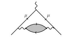
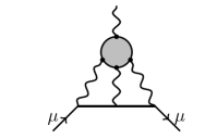
Figure 1: Hadronic contributions to $a_{\mu}$: The hadronic vacuum polarisation (left) and the hadronic light-by-light scattering (right).

A comparison of the Standard Model prediction of $a_{\mu}$ (cf. table 1) and the experimental determination reveals a deviation of about $3.5\sigma$, which could potentially hint to new physics. Further investigation requires both, the experimental as well as the theoretical uncertainties to be reduced. To match the targeted precision of the upcoming experiments ($\approx 1.5\times 10^{-10}$), this requires knowledge of the HVP contribution at the level of $0.2\%$ accuracy and the HLBL contribution at a level of about $10\%$.

In recent years a lot of effort has been undertaken to calculate the hadronic contributions to the anomalous magnetic moment of the muon from first principles using Lattice QCD. In the remainder of this proceedings I will review the current status of such lattice calculations and discuss the prospects and challenges to match the precision of the upcoming experiments.

2 Hadronic Vacuum Polarisation

Currently the most precise determinations of the HVP contribution to $a_{\mu}$ are obtained by using a dispersion relation and experimental data for the cross section $\sigma(e^{+}\,e^{-}\rightarrow\textnormal{hadrons})$ as an input

$$a_{\mu}^{\textnormal{\scriptsize HVP}}=\left(\frac{\alpha m_{\mu}}{3\pi}\right)^{2}\int\limits_{m^{2}_{\pi}}^{\infty}\textnormal{d}s\,\frac{R(s)K(s)}{s^{2}}\hskip 42.67912pt\textnormal{with}\qquad R(s)=\frac{\sigma(e^{+}\,e^{-}\rightarrow\textnormal{hadrons},s)}{\sigma(e^{+}\,e^{-}\rightarrow\mu^{+}\mu^{-},s)}$$ (2)

with an analytically known kernel function $K(s)$. Recent determinations of $a_{\mu}^{\textnormal{\scriptsize HVP}}$ from this method can be found in [6, 7, 8] and have a precision of about $0.5\%$. However, this approach relies on experimental input and an ab initio calculation can be done using lattice QCD.

2.1 The HVP from the Lattice

In the following we will discuss how the HVP contribution to $a_{\mu}$ can be calculated using lattice QCD. The hadronic vacuum polarisation tensor

$$\Pi_{\mu\nu}(Q)\equiv\int\!\textnormal{d}^{4}x\,\,e^{i\,Q\cdot x}\,\left<j^{\gamma}_{\mu}(x)\,\,j^{\gamma}_{\nu}(0)\right>=(Q_{\mu}Q_{\nu}-\delta_{\mu\nu}Q^{2})\,\Pi(Q^{2})\,,$$ (3)

is given by the four-dimensional Fourier transform of the correlation of two electromagnetic currents

$$j^{\gamma}_{\mu}=\frac{2}{3}\overline{u}\gamma_{\mu}u-\frac{1}{3}\overline{d}\gamma_{\mu}d-\frac{1}{3}\overline{s}\gamma_{\mu}s+\frac{2}{3}\overline{c}\gamma_{\mu}c\,,$$ (4)

which receive contributions from the different quark flavours multiplied by the respective charge factors. The contribution to the anomalous magnetic moment can then be determined from the vacuum polarisation function $\Pi(Q^{2})$ as [12]

$$a_{\mu}^{\textnormal{\scriptsize HVP}}=\left(\frac{\alpha}{\pi}\right)^{2}\int\limits_{0}^{\infty}\textnormal{d}Q^{2}\,K(Q^{2})\,\hat{\Pi}(Q^{2})\hskip 25.6073pt\textnormal{with}\hskip 11.38092pt\hat{\Pi}(Q^{2})=4\,\pi^{2}\left[\Pi(Q^{2})-\Pi(0)\right]\,.$$ (5)

with an analytically known electromagnetic kernel function $K(Q^{2})$. In the last few years it has become common to calculate the subtracted vacuum polarisation $\hat{\Pi}(Q^{2})$ required in equation (5) directly from the vector-vector two-point function $C(t)$ projected to zero spatial momentum [13, 14]

$$\hat{\Pi}(Q^{2})=4\pi^{2}\!\!\!\int\limits_{0}^{\infty}\!\!\textnormal{d}t\,C(t)\!\left[\!\frac{\cos(Qt)\!-\!1}{Q^{2}}+\frac{1}{2}t^{2}\right]\hskip 28.45274pt\textnormal{with}\qquad C(t)=\frac{1}{3}\sum\limits_{k=0}^{2}\sum\limits_{\vec{x}}\left<j^{\gamma}_{k}\!(\vec{x},t)j^{\gamma}_{k}\!(0)\right>\,.$$ (6)

Changing the order of integration one can obtain $a_{\mu}$ directly from $C(t)$ by integrating over the Euclidean time using the appropriate kernel function $f(t)$

$$\hskip 17.07182pta_{\mu}^{\textnormal{\scriptsize HVP}}\!=\!\!\!\int\limits_{0}^{\infty}\!\!\textnormal{d}t\,f(t)C(t)\,.$$ (7)

In isospin symmetric QCD the vector two-point function can be written in the following flavour decomposition

$$C(t)=\frac{5}{9}C^{\ell}(t)+\frac{1}{9}C^{s}(t)+\frac{4}{9}C^{c}(t)+C^{\textnormal{\scriptsize disc}}(t)\,,$$ (8)

with connected contributions for the light quark $C^{\ell}$, strange quark $C^{s}$ and charm $C^{c}$ quark as well as a quark-disconnected contribution $C^{\textnormal{\scriptsize disc}}$. The diagrams corresponding to the quark-connected and quark-disconnected Wick contractions are shown in figure 2.

Figure 2: Quark-connected (left) and quark-disconnected (right) Wick contraction for the HVP.

In the following, I will discuss the contributions to $a_{\mu}^{\textnormal{\scriptsize HVP}}$ flavour by flavour, starting with the light-quark connected contribution in section 2.2, followed by the strange- and charm-quark connected contributions in section 2.3, quark-disconnected contributions in section 2.4 and finally isospin breaking corrections in section 2.5. A summary and comparison of the various available results for $a_{\mu}^{\textnormal{\scriptsize HVP}}$ as well as an outlook for this quantity is given in section 2.6.

2.2 Light-Quark Contribution

In this section, I will show results for the light-quark connected contribution to $a_{\mu}^{\textnormal{\scriptsize HVP}}$ and discuss some of the main challenges for achieving a sub-percent precision calculation, namely the long distance noise-to-signal problem, finite volume corrections and accurate scale setting.

2.2.1 Long-Distance tail of the Vector Correlator

Figure 3 shows examples for the light-quark vector-vector two-point function $C(t)$ from the HPQCD/Fermilab/MILC [15] collaboration (left) and the integration kernel $f(t)\cdot C(t)$ for $a_{\mu}^{\textnormal{\scriptsize HVP}}$ from Mainz [16] (right). Both data sets have been obtained at physical pion mass.

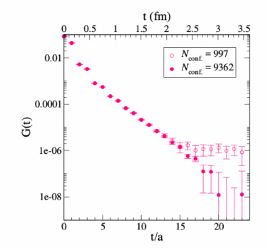
Figure 3: The vector correlator at physical pion mass: The plot on the left is from [15] and shows the two-point function $C(t)$ for two ensembles with the same parameters and different statistics. The plot on the right is from [16] and shows the integration kernel $f(t)\cdot C(t)$ for $a_{\mu}^{\textnormal{\scriptsize HVP}}$ with the light-quark contribution shown in black.

As one can see in both plots, the signal in the vector two-point function deteriorates for large Euclidean times $t$. The statistical error on the raw data can be improved by using noise reduction techniques such as all-mode-averaging [17, 18] or low-mode-averaging, which has been successfully used in [19, 20]. However, the statistical uncertainty for $a_{\mu}^{\textnormal{\scriptsize HVP}}$ after integrating the raw data of $C(t)$ over $t$ will still be dominated by the noise from large times. A possible approach to reduce this uncertainty, is to replace the correlator by a (multi-) exponential fit for $t>t_{c}$ (see, e.g., [22, 15]). A more systematic way to treat the long distance tail of the correlator is the bounding method [23, 19], which will be discussed in the following.

2.2.2 Bounding Method

The vector correlator can be written using the spectral representation as the sum of exponentials with positive prefactors

$$C(t)=\sum_{n}\frac{A^{2}_{n}}{2E_{n}}e^{-E_{n}t}\hskip 34.14322pt\textnormal{with}\qquad A_{n}^{2}>0\,.$$ (9)

The idea of the bounding method is to bound the two-point function $C(t)$ for Euclidean times larger than some value $t_{c}$ from above and below [23, 19]

$$0<C(t_{c})\,e^{-E_{t_{c}}(t-t_{c})}\leq C(t)\leq C(t_{c})\,e^{-E_{0}(t-t_{c})}\hskip 28.45274pt\textrm{for}\qquad t\geq t_{c}\,.$$ (10)

As a trivial lower bound one can use zero, since the correlator (cf. equation (9)) is strictly positive. A more stringent lower bound for $t\geq t_{c}$ can be obtained by using the effective mass $E_{t_{c}}$ at the given $t_{c}$. Since energy states with higher energies decay faster, the true correlator $C(t)$ is guaranteed to fall slower than $C(t_{c})\,e^{-E_{t_{c}}(t-t_{c})}$ for $t\geq t_{c}$. On the other hand, the true correlator is guaranteed to decay faster than the actual ground state energy $E_{0}$, and thus $C(t)\leq C(t_{c})\,e^{-E_{0}(t-t_{c})}$ is an upper bound for the correlator. In the vector channel, the ground state energy $E_{0}$ is given by the finite volume energy of two pions with one unit of momentum. When calculating $a_{\mu}^{\textnormal{\scriptsize HVP}}$ one now replaces the correlator for $t\geq t_{c}$ by the upper and the lower bound and varies $t_{c}$. An example of $a_{\mu}^{\textnormal{\scriptsize HVP}}$ plotted against $t_{c}$ is shown on the left-hand side of figure 4. As one can see, once $t_{c}$ is large enough, the result using the upper and lower bound overlap, and $a_{\mu}^{\textnormal{\scriptsize HVP}}$ can be extracted from this region.

Figure 4: $a_{\mu}^{\textnormal{\scriptsize HVP}}$ from the bounding method (left) and the improved bounding method (right) plotted against $t_{c}$. The plots are taken from [16] and use a pion mass of $M_{\pi}\approx 200$ MeV.

The bounding method can be further improved [16, 24] if a dedicated spectroscopy study for the vector channel is available. This requires to calculate two-point functions using various operators that have overlap with two-pion states. With the Generalised Eigenvalue Problem (GEVP) [25], one can extract the energies $E_{n}$ and overlap factors $A_{n}$ for the lowest $N$ states of the spectrum. Once these energies and overlap factors have been determined, the long-distance tail of the vector correlator can be reconstructed. An example at physical pion mass is shown in figure 5. As one can see, the more states are used in the reconstruction, the closer the reconstructed data are to the original correlator (shown in black in figure 5).

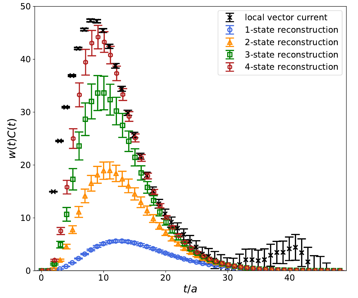
Figure 5: The integration kernel $f(t)\cdot C(t)$ for $a_{\mu}^{\textnormal{\scriptsize HVP}}$ plotted against $t$. The black data show the original correlator, the coloured points are reconstructions of the vector two-point function using one (blue) and up to four (red) states from the GEVP. The figure is taken from [24].

These reconstructed states can now be used to improve the bounding method as follows. Subtract the lowest $N$ states from the correlation function and bound the subtracted correlator $\tilde{C}(t)$

$$\tilde{C}(t)=C(t)-\sum_{n=0}^{N-1}\frac{A^{2}_{n}}{2E_{n}}e^{-E_{n}t}\hskip 54.06006pt0\leq\tilde{C}(t_{c})\,e^{-E_{t_{c}}(t-t_{c})}\leq\tilde{C}(t)\leq\tilde{C}(t_{c})\,e^{-E_{N}(t-t_{c})}\,.$$ (11)

Here, the upper bound is obtained using the energy of the $(N+1)$th state, i.e. the lightest state that was not subtracted from the correlator. The right-hand side of figure 4 shows the improved bounding method from [16] with the two lightest states subtracted. As one can see in comparison with the unimproved bounding method (left on figure 4) the upper and the lower bound now overlap at much smaller $t_{c}$ and $a_{\mu}^{\textnormal{\scriptsize HVP}}$ can be extracted with a smaller error.

2.2.3 Finite Volume Effects

Finite volume (FV) effects in the vector correlator are dominated by the two-pion state and can thus be expected to be important for large time separations $t$. Various studies (see, e.g. [26, 20, 16, 27]) of FV effects for lattice calculations of $a_{\mu}^{\textnormal{\scriptsize HVP}}$ suggest that these are of the order of $\Delta^{\textnormal{\scriptsize FV}}a_{\mu}^{\textnormal{\scriptsize HVP}}\approx 20-30\times 10^{-10}$ for typical sizes of $5-6$ fm of state-of-the-art lattice ensembles used at the physical point. Thus, it is crucial to carefully study and correct for FV effects when aiming at percent level precision for the HVP.

A straightforward way to study finite volume effects is using ensembles that differ only in the volume. Figure 6 shows results from the PACS collaboration [26] for the $a_{\mu}^{\textnormal{\scriptsize HVP}}$ integrand calculated using two different volumes of $5.4$ fm and $10.8$ fm at the physical pion mass. One can clearly see, a significant difference between the data on both ensembles, in particular for larger values of $t$. The authors of [26] found finite volume effects for $a_{\mu}^{\textnormal{\scriptsize HVP}}$ to be about $1.7$ times larger than what was expected from next-to-leading order (NLO) Chiral Perturbation Theory ($\chi$PT).

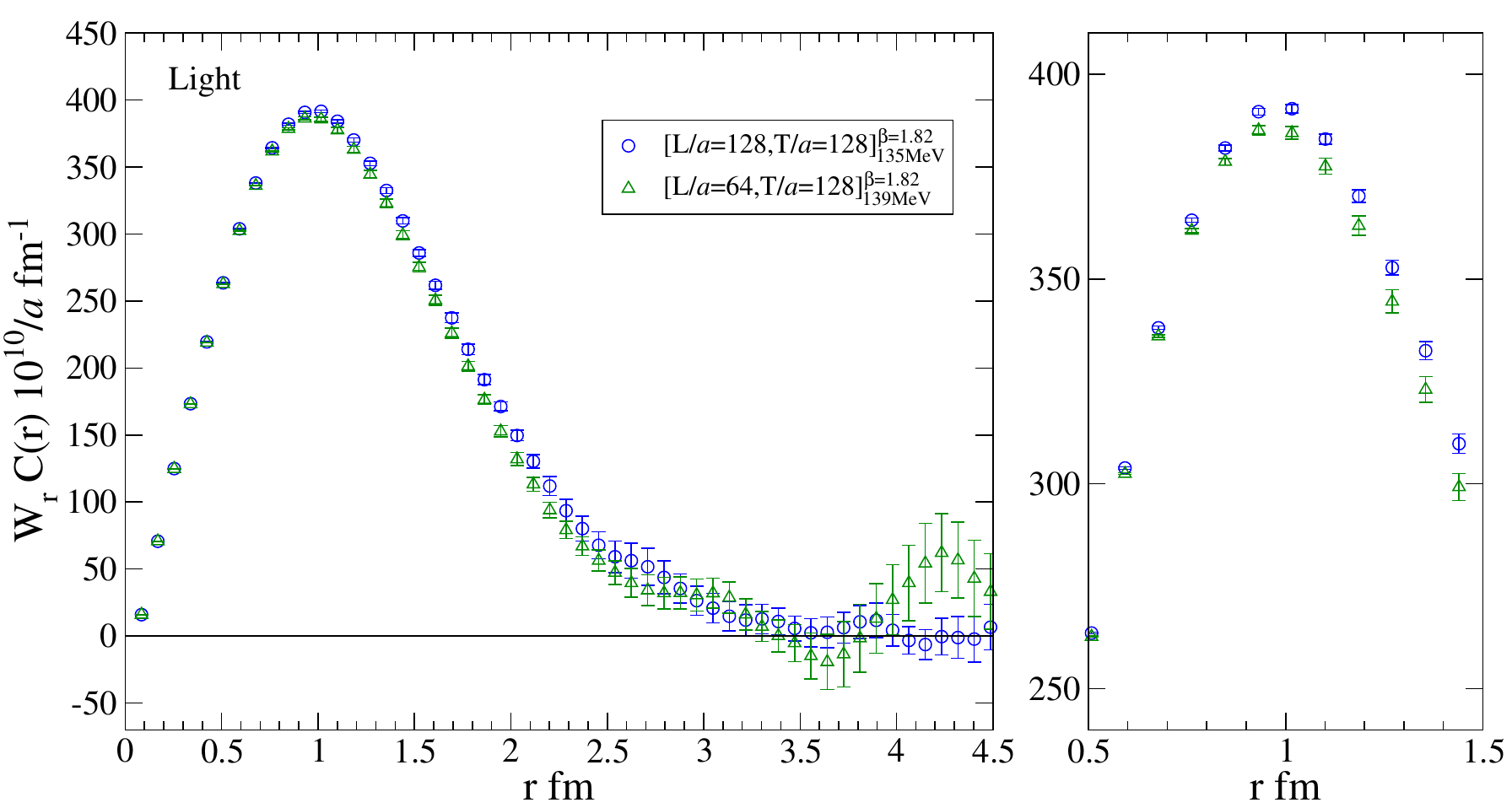
Figure 6: The $a_{\mu}^{\textnormal{\scriptsize HVP}}$ integrand calculated using two different volumes of $5.4$ fm (green triangles) and $10.8$ fm (blue circles) at physical pion mass. The plot on the right shows a zoomed-in version of the data on the left. The plot is taken from [26].

Finite volume corrections to $a_{\mu}^{\textnormal{\scriptsize HVP}}$ have been determined at next-to-next-to-leading order (NNLO) in $\chi$PT recently [28, 20] and the authors of [20] find that additional FV effects from NNLO are about $0.4-0.45$ times the NLO FV corrections.

A systematic way to study and correct for FV effects for the HVP is by writing the long distance contribution of the vector two-point function in terms of the timelike pion form factor. In [29, 30] it was suggested to use the Gounaris-Sakurai parameterization of the timelike pion form factor to calculate the infinite volume long-distance vector two-point function and the finite volume equivalent using the Gounaris-Sakurai parameterization combined with the Lellouch-Lüscher formalism [31, 32]. This approach has been used by Mainz [16], ETMC [33] and RBC/UKQCD [27] to study FV volume corrections and results after correcting for FV effects are found to be consistent when comparing ensembles that only differ by volume [16, 33]. The plot on the left-hand side of figure 7 is from Mainz [16] and shows the $a_{\mu}^{\textnormal{\scriptsize HVP}}$ integrand for two different ensembles at the same pion mass $M_{\pi}=280$ MeV with different volumes. The smaller volume is shown without (black circles) and with (blue squares) FV correction using the timelike pion form factor. After the data on the smaller ensemble has been corrected the results for the two different volumes agree with each other. The plot on the right-hand side of figure 7 is from ETMC [33] and shows $a_{\mu}^{\textnormal{\scriptsize HVP}}$ plotted against the pion mass for various ensembles without (open symbols) and with (closed symbols) FV corrections. In addition to using the timelike pion form factor to estimate FV effects for large times $t$, the authors of [33] use perturbative QCD for small $t$ to correct for FV effects. At a pion mass of around $M_{\pi}=320$ MeV, where several ensembles are available that only differ in volume, results are found to be in agreement once FV effects have been corrected for.

Figure 7: Correcting finite volume effects with the timelike pion form factor. The plot on the left is taken from [16] and shows the $a_{\mu}^{\textnormal{\scriptsize HVP}}$ integrand for two different ensembles at the same pion mass $M_{\pi}=280$ MeV with different volumes. The smaller volume is shown without (black circles) and with FV correction (blue squares). The plot on the right is taken from [33] and shows $a_{\mu}^{\textnormal{\scriptsize HVP}}$ vs the pion mass for various ensembles without (open symbols) and with (closed symbols) FV corrections.

In a recent paper [35], FV corrections to the HVP have been studied using a Hamiltonian approach, currently quoting corrections at $\mathcal{O}(e^{-m_{\pi}L})$, but neglecting effects of $\mathcal{O}(e^{-\sqrt{2}m_{\pi}L})$ and higher orders.

2.2.4 Scale Setting

Although $a_{\mu}$ is a dimensionless quantity, it depends on the scale of a given lattice, since the evaluation of the Kernel function for integrating the HVP requires to input the muon mass in lattice units. Assuming the scale has been set by some quantity $\Lambda$ with statistical error $\Delta\Lambda$, using error propagation one can show [22], that the relative error on $\Lambda$ is going to be enhanced by a factor of $\approx 1.8$ for $a_{\mu}^{\textnormal{\scriptsize HVP}}$

$$\Delta a_{\mu}^{\textnormal{\scriptsize HVP}}=\left|\Lambda\,\,\frac{\textrm{d}a_{\mu}^{\textnormal{\scriptsize HVP}}}{\textrm{d}\Lambda}\right|\cdot\,\frac{\Delta\Lambda}{\Lambda}=\left|M_{\mu}\frac{\textrm{d}a_{\mu}^{\textnormal{\scriptsize HVP}}}{\textrm{d}M_{\mu}}\right|\cdot\frac{\Delta\Lambda}{\Lambda}\hskip 56.9055pt\textnormal{with}\qquad M_{\mu}=\frac{m_{\mu}}{\Lambda}\,.$$ (12)

Thus, achieving $0.2\%$ accuracy on the HVP requires knowledge of the lattice scale to at least $0.1\%$. A suitable quantity for high-precision scale setting might be the mass of the $\Omega$-Baryon. However, whether or not scale setting at $0.1\%$ accuracy is possible in the near future remains to be investigated.

2.2.5 Comparison of Results for the Light-Quark Contribution

Figure 8 shows a comparison of results for the light-quark connected contribution to the HVP from various collaborations. The two different panels $N_{f}=2+1$ and $N_{f}=2+1+1$ denote the number of dynamical fermions used in the calculations.

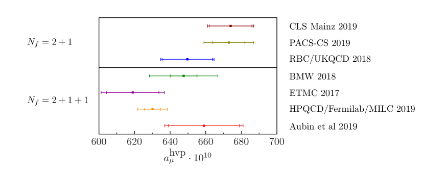
Figure 8: Comparison of lattice results for the light-quark contribution to $a_{\mu}^{\textnormal{\scriptsize HVP}}$. The values are taken from CLS Mainz 2019 [16], PACS-CS 2019 [26], RBC/UKQCD 2018 [19], BMW 2018 [36], ETMC 2018 [33], HPQCD/Fermilab/MILC 2019 [15], Aubin et al 2019 [20].

The relative errors on the light-quark contributions of the different results are about $1.3\%$ to $3.3\%$. For most of the collaborations, the error is dominated by statistics (inner error bar on the points in figure 8). As discussed above, the main challenge in terms of statistical error is the growing noise-to-signal ratio for large Euclidean time separations. Thus, a reduction of this error requires good control of the long-distance tail. A very promising approach for reaching sub-percent precision on the light quark contribution in the future is the improved bounding method discussed above.

As one can see, there is a slight tension between the smallest and the largest results of about $2\sigma$. This tension has to be object of further investigations, and in particular needs to be monitored when the collaborations further reduce the uncertainties in the individual calculations. A possible approach for determining the source of potential differences between different groups would be the comparison of more intermediate results, e.g. time-moments [37] of the vector correlator or $a_{\mu}$ calculated from a time window [19].

2.3 Strange- and Charm-Quark Contribution

The connected strange- and charm-quark contributions to the HVP are significantly smaller than the light-quark contribution and suffer far less from noise-to-signal problems in the long-distance tail or finite volume corrections. For the charm-quark contribution discretization effects can be large and lattice calculations should ideally include at least three different lattice spacings to reliably extrapolate to the continuum.

The results for the connected strange- and charm-quark contribution to $a_{\mu}^{\textnormal{\scriptsize HVP}}$ from various collaborations are shown in figure 9 and are in good agreement with each other. The errors correspond to errors of about $\lesssim 0.4\%$ and $\lesssim 0.3\%$ on the total HVP for the strange and charm, respectively. Thus, these contributions are already in a good shape when aiming at sub-percent precision for $a_{\mu}^{\textnormal{\scriptsize HVP}}$ from a lattice calculation.

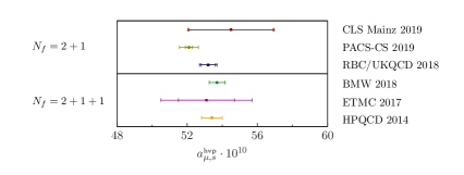
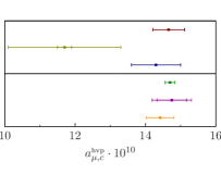
Figure 9: Comparison of lattice results for the strange-quark (left) and charm-quark (right) contributions to $a_{\mu}^{\textnormal{\scriptsize HVP}}$. Results are taken from CLS Mainz 2019 [16], PACS-CS 2019 [26], RBC/UKQCD 2018 [19], BMW 2018 [36], ETMC 2017 [38], HPQCD/Fermilab/MILC 2014 [37].

2.4 Quark-Disconnected Contribution

Besides the quark-connected contributions discussed above, the HVP receives a contribution from a quark-disconnected Wick contraction (cf. right-hand side of figure 2). The calculation of the respective disconnected quark-loops requires knowledge of the propagator from all lattice points to all other lattice points (all-to-all propagator), which has to be determined stochastically and is thus notoriously noisy. The combined light- and strange-quark disconnected contribution is $SU(3)$-flavour suppressed, i.e. it would vanish if $m_{s}=m_{\ell}$. In [39] it was shown that a substantial reduction in the statistical error can be achieved by exactly implementing $SU(3)$ suppression in the lattice calculation

$$C^{\textnormal{disc}}(t)=\frac{1}{9}\left<(\Delta^{\ell}(t)-\Delta^{s}(t))\cdot(\Delta^{\ell}(0)-\Delta^{s}(0))\right>\hskip 28.45274pt\textrm{with}\hskip 14.22636pt\Delta_{\mu}^{f}(t)=\sum_{\vec{x}}\textnormal{Tr}\left[\gamma_{\mu}S^{f}(x,x)\right]$$ (13)

and stochastically estimate the difference $\Delta^{\ell}(t)-\Delta^{s}(t)$ rather than the individual quark loops. Various stochastic estimators for $\Delta^{\ell}(t)-\Delta^{s}(t)$ and further noise reduction techniques have been proposed, e.g. low-mode-averaging and sparsened noise sources [40], hierarchical probing [41, 16] or frequency-splitting estimators [42, 43].

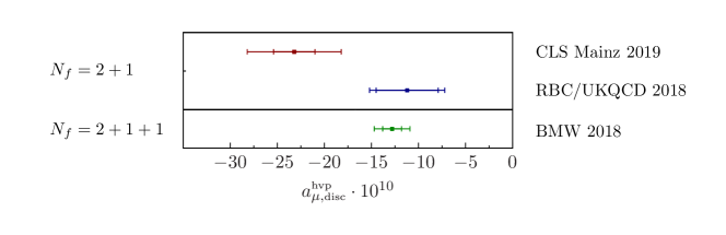
Figure 10: Comparison of lattice results for the quark-disconnected contribution to $a_{\mu}^{\textnormal{\scriptsize HVP}}$. Values are taken from CLS Mainz 2019 [16], RBC/UKQCD 2018 [19], BMW 2018 [36].

Figure 10 shows the published results for the quark-disconnected contribution to $a_{\mu}^{\textnormal{\scriptsize HVP}}$. The results are in reasonable agreement, although the results from Mainz is about $2\sigma$ below the two other values. Whether this is due to the chiral extrapolation done in [16] needs to be investigated by adding data closer or at the physical point in this calculation.

The errors on the available published results for the quark-disconnected contribution correspond to errors of about $0.3-0.7\%$ on the total HVP and thus, are already precise enough for a $1\%$ determination of $a_{\mu}^{\textnormal{\scriptsize HVP}}$, however, still need to be improved if an error of $<0.2\%$ is targeted.

Work in progress on calculating the quark-disconnected contribution to the hadronic vacuum polarisation by the HPQCD/Fermilab/MILC collaboration was presented at this conference [44].

2.5 Isospin Breaking Corrections

All lattice calculations discussed above have been done in the isospin symmetric limit, where the up- and the down-quark are treated as being equal. However, in nature, isospin is broken by the different electromagnetic charges of the up- and the down-quark as well as their different bare quark masses. These effects are expected to be of the order of $\mathcal{O}(\alpha)\approx 1\%$ and $\mathcal{O}((m_{d}-m_{u})/\Lambda_{\textnormal{\scriptsize QCD}})\approx 1\%$, respectively. Clearly, a lattice calculation aiming at such precision will need to include these effects. It is important to stress that the separation of strong isospin breaking and QED effects require to define a renormalisation prescription. At the same time the definition of the “physical” point in a pure QCD simulation becomes scheme dependent. Only in full QCD$+$QED with $m_{u}\neq m_{d}$ the physical point is unambiguously defined, e.g. by matching a set of hadron masses to their experimental value (see e.g. [46]).

2.5.1 Strong Isospin Breaking Correction

The effect from strong isospin breaking can be taken into account in a lattice calculation by simply using different input quark masses for the up and the down quark. This has been done for calculating the strong isospin breaking correction to the HVP by the HPQCD/Fermilab/MILC collaboration [47]. Here, two different gauge ensembles where used, one with $N_{f}=2+1+1$ and $m_{u}\neq m_{d}$ only in the valance sector and one with $N_{f}=1+1+1+1$ taking also strong isospin breaking corrections for the sea quarks into account. The strong isospin breaking correction is then quoted as the difference between calculating $a_{\mu}^{\textnormal{\scriptsize HVP}}$ using the average up- and down-quark mass for the light quarks and using the up-quark mass for the up and the down-quark mass for the down quark. In [47] the authors find $\delta^{sIB}a_{\mu}^{\textnormal{\scriptsize HVP}}=(7.7\pm 3.7)\times 10^{-10}$ and $\delta^{sIB}a_{\mu}^{\textnormal{\scriptsize HVP}}=(9.0\pm 2.3)\times 10^{-10}$ using the ensemble without and with $m_{u}\neq m_{d}$ for the sea quarks, respectively.

A different approach for including strong isospin breaking corrections in a lattice calculation is by expanding [48] the path integral in the difference of the respective quark masses and their isospin symmetric mass $\hat{m}$

$$\left<O\right>_{m_{f}\neq\hat{m}_{f}}=\left<O\right>_{m_{f}=\hat{m}}+\Delta m_{f}\left.\frac{\partial}{\partial m_{f}}\left<O\right>\right|_{m_{f}=\hat{m}}+\mathcal{O}\left(\Delta m_{f}^{2}\right)$$ (14)

with $\Delta m_{f}=m_{f}-\hat{m}$. At $\mathcal{O}(\Delta m_{f})$ one has to calculate contributions with one insertion of a scalar current. The corresponding diagrams for the hadronic vacuum polarisation are shown in figure 11. Diagram $M$ and $O$ are the correction for the valance quarks for the quark-connected and quark-disconnected HVP, respectively, whereas diagrams $R$ and $R_{d}$ correspond to sea-quark effects.

Figure 11: Mass insertion diagrams for the hadronic vacuum polarisation. The insertion of a scalar current is denoted by the diamond-shaped vertex.

The expansion of the path integral was used in [49, 19] to calculate the valance effect for the quark-connected HVP (diagram $M$). The ETMC collaboration finds $\delta^{sIB}a_{\mu}^{\textnormal{\scriptsize HVP}}=(6.0\pm 2.3)\times 10^{-10}$ [49] and RBC/UKQCD obtains $\delta^{sIB}a_{\mu}^{\textnormal{\scriptsize HVP}}=(10.6\pm 4.3\pm 6.6)\times 10^{-10}$ [19].

2.5.2 QED Correction

The determination of electromagnetic corrections requires the inclusion of QED when evaluating the Euclidean path integral. Since QED is a long range interaction, finite volume (FV) effects for lattice calculations can be large. Compared to pure QCD, where FV corrections are exponentially suppressed, in the case of QED finite volume corrections are usually power-law. For QED_L [50], which is a commonly used prescription of QED in a finite volume, all the spatial zero modes of the photon field are subtracted and finite volume effects for the QED corrections to the HVP are of $\mathcal{O}(1/(m_{\pi}L)^{3})$ [52, 53, 38], and thus negligible within the required precision for the HVP when using typical lattice sizes with $m_{\pi}L\gtrsim 4$.

Since the electromagnetic fine structure constant $\alpha$ is small at low energies, QED can be treated in a perturbative way by expanding the QCD$+$QED path integral in $e^{2}$ [54]

$$\left<O\right>_{\textnormal{\scriptsize QCD}+\textnormal{\scriptsize QED}}=\left<O\right>_{\textnormal{\scriptsize QCD}}+\frac{1}{2}\,e^{2}\left.\frac{\partial^{2}}{\partial e^{2}}\left<O\right>\right|_{e=0}+{\cal{O}}(\alpha^{2})\,.$$ (15)

At $\mathcal{O}(\alpha)$ this requires to calculate diagrams that include one photon propagator. The respective diagrams for the HVP are shown in figure 12. Diagrams $S$ and $V$ are QED corrections to the quark-connected HVP and diagrams $F$ and $D3$ are QED corrections to the quark-disconnected HVP. All other diagrams correspond to QED effects for the sea quarks.

Figure 12: QED correction diagrams for the hadronic vacuum polarisation.

The ETMC [49] and RBC/UKQCD collaborations [19, 55] both have calculated QED corrections to the quark-connected HVP in the electro-quenched approximation, where QED corrections for the sea-quarks are not taken into account. Calculating QED corrections at various masses heavier than physical pion mass and extrapolating to the physical point, ETMC finds $\delta^{\textnormal{\scriptsize QED}}a_{\mu}^{\textnormal{\scriptsize HVP}}=1.1(1.0)\times 10^{-10}$ [49]. RBC/UKQCD finds $\delta^{\textnormal{\scriptsize QED}}a_{\mu}^{\textnormal{\scriptsize HVP}}=5.9(5.7)\times 10^{-10}$ [19], consistent with ETMC albeit with larger error bars, working directly at physical masses at a single lattice spacing. Further work in progress for QED corrections to the HVP by other collaborations was presented at this conference [56, 57].

The leading QED correction to the quark-disconnected HVP is given by the diagram $F$ shown in figure 12. Other than the same diagram without the photon connecting the two quark loops (i.e. the pure QCD quark-disconnected diagram), this contribution is not $SU(3)$-flavour suppressed and could thus be important. When calculating this contribution, one is only interested in the case where, besides the photon line, the quark-loops are in addition connected by gluons. If no additional gluons connect the quarks, these contributions are conventionally included in the NLO HVP contribution to $a_{\mu}$ (cf. table 1) and thus, need to be subtracted in a lattice calculation to avoid double counting. RBC/UKQCD calculated this diagram and finds $\delta^{\textnormal{\scriptsize QED, disc}}a_{\mu}^{\textnormal{\scriptsize HVP}}=-6.9(2.1)(1.4)\times 10^{-10}$ [19].

The diagrams in figure 12 corresponding to sea-quark effects are all at least either $SU(3)$-flavour or $1/N_{c}$ suppressed. However, naively, they could still be of the order of $\approx 33\%$ of the connected contribution. Thus, when aiming at sub-percent precision for the total HVP contribution to $a_{\mu}$, these effects will have to be included eventually.

2.6 Summary - HVP Contribution to $a_{\mu}$

Figure 13 shows a comparison of results for the total HVP contribution to $a_{\mu}$. The upper panel shows determinations using the $R$-ratio data. The coloured points in the panel labeled “lattice” shows the published lattice results from various collaboration. The lowest point in the plot (“no new physics”) denotes the result when subtracting all other Standard Model contributions (as in table 1) from the experimental result, i.e. the value that $a_{\mu}^{\textnormal{\scriptsize HVP}}$ would have to take for the Standard Model prediction to be in agreement with experiment. Clearly, at the current state-of-the-art, lattice calculations are not yet precise enough to distinguish between the $R$-ratio results and the “no new physics” scenario.

Furthermore, one can see that the smallest and largest lattice results disagree at a level of about $2\sigma$. Slight tensions between lattice results will have to be subject to further investigation in the future, in particular once the collaborations reduce the errors, to make sure to achieve consensus between the various lattice results. A possible approach is the comparison of more intermediate quantities, e.g. time-moments [37] of the vector correlator or $a_{\mu}^{\textnormal{\scriptsize HVP}}$ calculated from a time window [19].

Finally, the point in the second panel in figure 13 shows a result from RBC/UKQCD [19] combining lattice and $R$-ratio results using a window method, where the vector correlator from small and large distances is taken from the $R$-ratio and intermediate distances from a lattice calculation. The point shown here uses the $R$-ratio data compilation from “Jegerlehner 2017” [59] and clearly shows that it is possible to improve the $R$-ratio results by supplementing it with data from a lattice calculation.

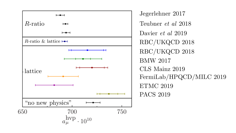
Figure 13: Comparison of various determinations of the HVP contribution to the anomalous magnetic moment of the muon.

The relative contribution of the various quark-flavours to the total HVP contribution from lattice calculations is shown by the pie chart on the left-hand side of figure 14. Clearly, the by far biggest contribution comes for the light-quark connected diagram, followed by the strange-quark contribution.

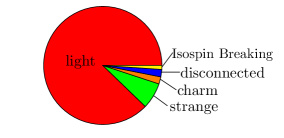
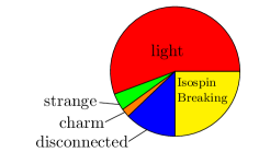
$a^{\textnormal{\scriptsize HVP}}_{\mu}$                                                                   $\delta a^{\textnormal{\scriptsize HVP}}_{\mu}$

Figure 14: The relative size of the various flavour contributions to the HVP is shown on the left. The plot on the right shows the relative size of the average (statistical + systematic) error on the various flavour contributions from the available lattice results.

The total errors on the lattice results for the HVP shown in figure 13 are all of the order of $2-3\%$. This is clearly not yet competitive with the $R$-ratio results, which would require an accuracy of $\lesssim 1\%$, or even the required $0.2\%$ to match the precision of the upcoming experiments. The relative contribution to the error on the average lattice calculation is shown in the pie chart on the right-hand side of figure 14. The error on the lattice results is dominated by the error on the light-quark contribution. The main challenges for reaching sub-percent precision for the light-quark contributions, that were discussed in previous sections, are controlling the statistical noise in the long-distance tail, having careful and reliable estimates of finite volume effects as well as a precise scale setting.

The second biggest contribution to the error on the average lattice calculation (cf. right-hand side of figure 14) comes from isospin breaking corrections (or the systematic error made by not including those effects). Given that the first calculations of isospin breaking corrections have only recently become available, progress and further reduction of statistical error is to be expected in the near future. However, it is also important to study the effects of including QED for the sea quarks, since these contributions could potentially be important at the level of sub-percent precision for the hadronic vacuum polarisation.

For the future, the first goal is to obtain calculations of $a_{\mu}^{\textnormal{\scriptsize HVP}}$ from lattice calculations at a precision of $\lesssim 1\%$, at which the lattice becomes competitive to $R$-ratio determinations. Given the recent progress presented at this conference, first results at $1\%$ precision could be available within the time frame of a year.

Besides the anomalous magnetic moment of the muon, the hadronic vacuum polarisation also enters in other quantities, like the running of the electromagnetic coupling and the running of the electroweak mixing angle. Progress in this direction was presented by Mainz at this conference  [60].

3 Hadronic Light-by-Light Scattering

The hadronic light-by-light scattering contribution (cf. diagram on the right-hand side of figure 1) enters the anomalous magnetic moment at order $\alpha^{3}$. The value that is often used for the Standard Model prediction is the so-called “Glasgow-consensus” [11], which includes model-dependent estimates of various contributions to the light-by-light scattering, with the largest contribution coming from the $\pi^{0}$-pole. Recent work in progress on dispersion relations for the hadronic light-by-light scattering can be found, e.g., in [61, 62, 63] and references therein.

In the following, I will discuss the progress of ab initio calculations of the hadronic light-by-light scattering using lattice QCD.

3.1 Light-by-Light from the Lattice

The hadronic part of the light-by-light scattering amplitude is written in terms of the expectation value of four electromagnetic currents

$$\Pi_{\mu\nu\lambda\rho}(q_{1},q_{2},q_{3})=\int\textnormal{d}^{4}x_{1}\textnormal{d}^{4}x_{2}\textnormal{d}^{4}x_{3}\,e^{-i(q_{1}x_{1}+q_{2}x_{2}+q_{3}x_{3})}\left<j^{\gamma}_{\mu}(x_{1})j^{\gamma}_{\nu}(x_{2})j^{\gamma}_{\lambda}(x_{3})j^{\gamma}_{\rho}(0)\right>\,.$$ (16)

The fully quark-connected as well as the leading quark-disconnected Wick contraction are shown in figure 15. All other possible quark-disconnected contractions are $SU(3)$-flavour suppressed.

Figure 15: Fully quark-connected (left) and leading quark-disconnected (right) contributions to the hadronic light-by-light scattering.

Currently, two collaborations – Mainz and RBC/UKQCD – are actively working on calculating the hadronic light-by-light scattering contribution $a_{\mu}^{\textnormal{\scriptsize HLBL}}$ to the anomalous magnetic moment of the muon from the lattice. Both collaborations use position space approaches and their methods and status are described in sections 3.2 and 3.3, respectively.

3.2 Mainz Status

In the position-space method developed by Mainz [64, 65] the hadronic light-by-light scattering contribution to $a_{\mu}$ is written as

$$a_{\mu}^{\textnormal{\scriptsize HLBL}}=\frac{m_{\mu}e^{6}}{3}\int\!\textnormal{d}x^{4}\textnormal{d}y^{4}\,\overline{\mathcal{L}}_{[\rho,\sigma];\mu\nu\lambda}(x,y)\,\,i\hat{\Pi}_{\rho;\mu\nu\lambda\sigma}(x,y)\,.$$ (17)

The hadronic part is given by the four-point function

$$\hat{\Pi}_{\rho;\mu\nu\lambda\sigma}=\int\!\textnormal{d}z^{4}\,\,iz_{\rho}\left<j^{\gamma}_{\mu}(x)\,j^{\gamma}_{\nu}(y)\,j^{\gamma}_{\lambda}(0)\,j^{\gamma}_{\sigma}(z)\right>$$ (18)

where $z$ is the position of the vertex with the external photon, and $x$, $y$ and $0$ the positions of the quark-photon vertices with the internal photon lines. The QED part of the light-by-light diagram is given by an electromagnetic kernel function $\overline{\mathcal{L}}_{[\rho,\sigma];\mu\nu\lambda}(x,y)$, that can be computed directly in the continuum and infinite volume limit.

Figure 16: The quark-connected contribution to $a_{\mu}^{\textnormal{\scriptsize HLBL}}$ for different pion masses. The data has been integrated up to $|y|_{\textnormal{\scriptsize max}}$. Plot is taken from [66].

The current status of calculating $a_{\mu}^{\textnormal{\scriptsize HLBL}}$ using this method was presented at this conference [66] and some results for the fully quark-connected contribution are shown in figure 16. The plot in figure 16 shows $a_{\mu}^{\textnormal{\scriptsize HLBL}}$ for three different pion masses at fixed lattice spacing. The data has been partially integrated up to $|y|_{\textnormal{\scriptsize max}}$, such that $a_{\mu}^{\textnormal{\scriptsize HLBL}}$ can be extracted from a plateau at large enough values of $|y|_{\textnormal{\scriptsize max}}$.

3.3 RBC/UKQCD Status

In the position space approach proposed by RBC/UKQCD [67] the full hadronic light-by-light scattering diagram including the muon and photon propagators is treated on the lattice. To make this calculation feasible, position space sampling is used, where the sum over the position of two of the quark-photon vertices is sampled stochastically. For the photon propagators RBC/UKQCD uses either the QED_L [50] prescription leading to power-law finite volume corrections or the infinite volume formulation (QED_∞) of the photon propagator as proposed in [68].

Figure 17 shows results from the recent paper [69] using QED_L for the photon propagator. $a_{\mu}^{\textnormal{\scriptsize HLBL}}$ obtained on various different gauge ensembles is plotted against $1/(m_{\mu}L)^{2}$ with the box size $L$ for the fully quark-connected diagram (left) and the leading quark-disconnected diagram (right). The lines in the plots show the infinite volume and continuum extrapolation with the purple point at $1/(m_{\mu}L)^{2}=0$ showing the result extrapolated to the infinite volume and continuum limit.

Figure 17: Infinite volume and continuum extrapolation of $a_{\mu}^{\textnormal{\scriptsize HLBL}}$ using QED_L for the photons for the fully connected diagram (left) and the leading disconnected diagram (right). In both plots the purple point at $1/(m_{\mu}L)^{2}=0$ shows the result extrapolated to infinite volume and continuum. The plots are taken from [69].

The quark-connected and leading quark-disconnected contribution are found to have opposite signs, and the result for the sum of both contribution is [69]

$$a_{\mu}^{\textnormal{\scriptsize HLBL}}=7.20(3.98)(1.65)\times 10^{-10}\,.$$ (19)

extrapolated to the physical point. The result (19) is consistent with the model estimates used in the Glasgow Concensus (cf. table 1), albeit with larger uncertainties.

In addition RBC/UKQCD presented progress [70, 71] on calculating $a_{\mu}^{\textnormal{\scriptsize HLBL}}$ using QED_∞ at this conference. The long-distance tail of the hadronic light-by-light scattering is dominated by the $\pi^{0}$-pole contribution (cf. diagram in figure 18). This can be used to further improve the calculation of $a_{\mu}^{\textnormal{\scriptsize HLBL}}$ by supplementing the long distance by the pion-pole contribution calculated either from a model or directly from the lattice using the pion transition form factor $\pi^{0}\rightarrow\gamma\gamma$ and work in progress in that direction was presented [70, 71].

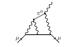
Figure 18: $\pi^{0}$ pole contribution to the hadronic light-by-light scattering

3.4 Summary

Currently two collaborations are actively working on determining the hadronic light-by-light scattering contribution to $a_{\mu}$ from first principles using lattice calculations. RBC/UKQCD has recently published [69] the first result extrapolated to the continuum and infinite volume limit and Mainz has presented [66] promising work in progress using their position space approach [64, 65].

For the hadronic light-by-light scattering contribution to explain the discrepancy between experimental measurement and Standard Model prediction of $a_{\mu}$, one would need a value which is about three times larger than the number quoted in the Glasgow consensus. However, current lattice calculations suggest, that this is very unlikely.

To match the precision of the upcoming experimental results for $g-2$, the hadronic light-by-light scattering amplitude needs to be determined to a precision of about $10\%$. A promising proposal to reduce the statistical noise from the long-distance contribution is to constrain lattice data at long distances by the pion-pole contribution. A lattice calculation of the pion-pole contribution requires the pion transition form factor $\pi^{0}\rightarrow\gamma\gamma$ (see [72, 73] for recent calculations from the Mainz collaboration).

4 Final Remarks

The persistent discrepancy between the Standard Model prediction (table 1) and the experimental result (equation (1)) for the anomalous magnetic moment of the muon has triggered a tremendous effort within the lattice community to calculate the hadronic contributions to $a_{\mu}$ from first principles. The upcoming experiments at Fermilab [2] and JPARC [3] aim to further reduce the uncertainty of the experimental result by a factor of $4$. To match the precision of these upcoming experiments one finally has to determine the hadronic vacuum polarisation contribution $a_{\mu}^{\textnormal{\scriptsize HVP}}$ to a precision of about $0.2\%$ and the hadronic light-by-light scattering $a_{\mu}^{\textnormal{\scriptsize HLBL}}$ to about $10\%$ accuracy.

In terms of the hadronic vacuum polarisation, which is the leading hadronic contribution to $a_{\mu}$, several results from different collaborations with a precision of $2-3\%$ are available and summarised in figure 13. Recent progress presented at this conference suggests, that the first results at around $1\%$ precision could be available within the time frame of a year.

References

- [1] G. W. Bennett et al., Phys.Rev. D73 (2006) 072003, [arXiv:hep-ex/0602035]
- [2] Fermilab E989 Collaboration, Nucl.Part.Phys.Proc. 273-275 (2016) 584-588, [arXiv:1411.2555]
- [3] E34 Collaboration, JPS Conf.Proc. 8 (2015) 025008
- [4] T. Kinoshita et al., Phys.Rev.Lett. 109 (2012) 111808, [arXiv:1205.5370]
- [5] C. Gnendiger, D. Stöckinger, H. Stöckinger-Kim, Phys.Rev. D88 (2013) 053005
- [6] A. Keshavarzi, D. Nomura, T. Teubner, Phys.Rev. D97 (2018) no.11, 114025, [arXiv:1802.02995]
- [7] M. Davier et al., arXiv:1908.00921
- [8] F. Jegerlehner, (2017), arXiv:1705.00263
- [9] K. Hagiwara et al., J.Phys. G38 (2011) 085003, [arXiv:1105.3149]
- [10] A. Kurz et al., Phys.Lett. B734 (2014) 144-147
- [11] J. Prades et al., Adv.Ser.Direct.High Energy Phys. 20 (2009) 303-317, [arXiv:0901.0306]
- [12] T. Blum, Phys.Rev.Lett. 91 (2003) 052001, [arXiv:hep-lat/0212018]
- [13] D. Bernecker and H. B. Meyer, Eur. Phys. J. A47, 148 (2011), [arXiv:1107.4388]
- [14] X. Feng et al., Phys.Rev. D88, 034505 (2013), [arXiv:1305.5878]
- [15] C. Davies et al., arXiv:1902.04223
- [16] A. Gérardin et al., Phys.Rev. D100 (2019) no.1, 014510, [arXiv:1904.03120]
- [17] T. Blum, T. Izubuci and E. Shintani, Phys.Rev. D88 (2013) no.9, 094503, [arXiv:1208.4349]
- [18] G. Bali, S. Collins and A. Schäfer, Comput.Phys.Commun. 181 (2010) 1570-1583, [arXiv:0910.3970]
- [19] T. Blum et al., Phys. Rev. Lett. 121, 022003 (2018), [arXiv:1801.07224]
- [20] C. Aubin et al., Phys.Rev. D101 (2020) no.1, 014503, [arXiv:1905.09307]
- [21] C. Aubin et al., PoS LATTICE2019 (2019), [arXiv:1910.05094]
- [22] M. Della Morte et al., JHEP 1710 (2017) 020, [arXiv:1705.01775]
- [23] Sz. Borsanyi et al., Phys.Rev. D96 (2017) no.7, 074507, [arXiv:1612.02364]
- [24] A. Meyer et al., PoS LATTICE2019 (2019), [arXiv:1910.11745]
- [25] B. Blossier et al., JHEP 0904 (2009) 094, [arXiv:0902.1265]
- [26] E. Shintani and Y. Kuramashi, Phys.Rev. D100 (2019) no.3, 034517, [arXiv:1902.00885]
- [27] C. Lehner, PoS LATTICE2019 (2019)
- [28] J. Bijnens and J. Relefors, JHEP 1712 (2017) 114, [arXiv:1710.04479]
- [29] H. Meyer, Phys.Rev.Lett. 107 (2011) 072002, [arXiv:1105.1892]
- [30] A. Francis et al., Phys.Rev. D88 (2013) 054502, [arXiv:1306.2532]
- [31] M. Lüscher, Nucl.Phys. B364 (1991) 237-251
- [32] L. Lellouch and M. Lüscher, Commun.Math.Phys. 219 (2001) 31-44, [arXiv:hep-lat/0003023]
- [33] D. Giusti et al., Phys.Rev. D98 (2018) no.11, 114504, [arXiv:1808.00887]
- [34] D. Giusti et al., PoS LATTICE2019 (2019), [arXiv:1910.03874]
- [35] M. Hansen and A. Patella, Phys.Rev.Lett. 123 (2019) 172001, [arXiv:1904.10010]
- [36] Sz. Borsanyi et al., Phys.Rev.Lett. 121 (2018) no.2, 022002, [arXiv:1711.04980]
- [37] B. Chakraborty et al., Phys.Rev. D89 (2014) no.11, 114501, [arXiv:1403.1778]
- [38] D. Giusti et al., JHEP 1710 (2017) 157, [arXiv:1707.03019]
- [39] V. Gülpers et al., PoS LATTICE2014 (2014) 128, [arXiv:1411.7592]
- [40] T. Blum et al., Phys.Rev.Lett. 116 (2016) no.23, 232002, [arXiv:1512.09054]
- [41] A. Stathopoulos, J. Laeuchli and K. Orginos, arXiv:1302.4018
- [42] L. Giusti et al., Eur.Phys.J. C79 (2019) no.7, 586, [arXiv:1903.10447]
- [43] T.Harris et al., PoS LATTICE2019 (2019), [arXiv:2001.08783]
- [44] C. E. DeTar et al., PoS LATTICE2019 (2019), [arXiv:1912.04382]
- [45] A. Gérardin et al., PoS LATTICE2019 (2019), [arXiv:1911.04733]
- [46] S. Aoki et al., FLAG Review 2019, [arXiv:1902.08191]
- [47] B. Chakraborty et al., Phys.Rev.Lett. 120 (2018) no.15, 152001, [arXiv:1710.11212]
- [48] G. M. de Divitiis et al., JHEP 04, 124 (2012), [arXiv:1110.6294]
- [49] D. Giusti et al., Phys.Rev. D99 (2019) no.11, 114502, [arXiv:1901.10462]
- [50] M. Hayakawa and S. Uno, Prog. Theor. Phys. 120, 413 (2008), [arXiv:0804.2044]
- [51] X. Feng and L. Jin, arXiv:1812.09817
- [52] J. Bijnens et al., Phys.Rev. D100 (2019) no.1, 014508, [arXiv:1903.10591]
- [53] N. Hermansson-Truedsson et al., PoS LATTICE2019 (2019), [arXiv:1910.03250]
- [54] G. M. de Divitiis et al., Phys.Rev. D87 (2013) no.11, 114505, [arXiv:1303.4896]
- [55] V. Gülpers et al., PoS LATTICE2018 (2018), [arXiv:1812.09562]
- [56] A. Risch and H. Wittig, PoS LATTICE2019 (2019), [arXiv:1911.04230]
- [57] Bálint Tóth, PoS LATTICE2019 (2019)
- [58] B. Chakraborty et al., Phys.Rev. D98 (2018) no.9, 094503, [arXiv:1806.08190]
- [59] F. Jegerlehner. 2017. alphaQEDc17, http://www-com.physik.hu-berlin.de/ fjeger/software.html
- [60] M. Cè et al., PoS LATTICE2019 (2019), [arXiv:1910.09525]
- [61] G. Colangelo et al., JHEP 1902 (2019) 006, [arXiv:1810.00007]
- [62] M. Hoferichter et al., Phys.Rev.Lett. 121 (2018) no.11, 112002, [arXiv:1805.01471]
- [63] V. Pauk and M. Vanderhaeghen, Phys.Rev. D90 (2014) no.11, 113012, [arXiv:1409.0819]
- [64] J. Green et al., PoS LATTICE2015 (2016) 109, [arXiv:1510.08384]
- [65] N. Asmussen et al., PoS LATTICE2016 (2016) 164, [arXiv:1609.08454]
- [66] N. Asmussen et al., PoS LATTICE2019 (2019), [arXiv:1911.05573]
- [67] T. Blum et al., Phys.Rev. D93 (2016) no.1, 014503, [arXiv:1510.07100]
- [68] T. Blum et al., Phys.Rev. D96 (2017) no.3, 034515, [arXiv:1705.01067]
- [69] T. Blum et al., arXiv:1911.08123
- [70] T. Blum et al., PoS LATTICE2019 (2019)
- [71] L. Jin et al., PoS LATTICE2019 (2019)
- [72] A. Gérardin et al., Phys.Rev. D94 (2016) no.7, 074507, [arXiv:1607.08174]
- [73] A. Gérardin et al., Phys.Rev. D100 (2019) no.3, 034520, [arXiv:1903.09471]