Abstract

By supplementing the pressure space for the Taylor–Hood element a triangular element that satisfies continuity over each element is produced. Making a novel extension of the patch argument to prove stability, this element is shown to be globally stable and give optimal rates of convergence on a wide range of triangular grids. This theoretical result is extended in the discussion given in the appendix, showing how optimal convergence rates can be obtained on all grids. Two examples are presented, one illustrating the convergence rates and the other illustrating difficulties with the Taylor–Hood element which are overcome by the element presented here.

Introduction

A popular triangular element for solving two-dimensional flows was introduced by Hood & Taylor [9]. It has the serious physical drawback that continuity is only satisfied over the whole domain of the problem and not over each element. A consequence of this phenomenon and the poor approximation that can result is given by Tidd, Thatcher & Kaye [11] and a further example of poor results is illustrated in section 6. Tidd et al. show that by supplementing the continuous linear pressure by functions constant in each element, not only is continuity satisfied locally but also the quality of the solution is greatly improved, at least for the particular problem that they were considering. This idea of supplementing the pressure space had previously been suggested by Gresho et al. [5] and is also discussed by Griffiths [7]. In this paper a stability analysis is presented which shows that this element is stable on a wide range of triangular grids. Details of the formulation of the continuous and discrete equations for Stokes flow and the implications of the analysis of Stokes flow for Navier–Stokes flow will not be given here. Only sufficient detail to introduce the notation is presented; for further details see Girault & Raviart [4].

The Stokes equations, in weak form, may be written

$$\text{find }(u,q)\in(H^{1}_{0}(\Omega))^{2}\times L^{2}_{0}(\Omega)$$ such that

$$\nu(\nabla u,\nabla v)_{\Omega}-(\operatorname{div}v,q)_{\Omega} =(f,v)_{\Omega}\quad\forall\,v\in(H^{1}_{0}(\Omega))^{2},$$ (1)

$$(\operatorname{div}u,p)_{\Omega} =0\quad\forall\,p\in L^{2}_{0}(\Omega),$$ (2)

where

1. $H^{1}_{0}(\Omega)=\{f\mid f\in H^{1}(\Omega),f=0\hbox{ on }\partial\Omega\}$,

2. $L^{2}_{0}(\Omega)=\{f\mid f\in L^{2}(\Omega),(f,1)_{\Omega}=0\}$,

3. $(f,g)_{\Omega}=\int_{\Omega}fg\,d\Omega$.

The discrete analogue of (1) and (2) in the finite element subspaces $V^{h}\subset(H^{1}_{0}(\Omega))^{2}$ and $P^{h}\subset L^{2}_{0}(\Omega)$ is given by

$$\text{find }(u^{h},q)^{h}\in V^{h}\times P^{h}\text{ such that}$$

$$\nu(\nabla u^{h},\nabla v^{h})_{\Omega}-(\operatorname{div}v^{h},q^{h})_{\Omega} =(f,v^{h})_{\Omega}\quad\forall\,v^{h}\in V^{h},$$ (3)

$$(\hbox{div\,}u^{h},p^{h})_{\Omega} =0\quad\forall\,p^{h}\in P^{h}.$$ (4)

The essential result for stability and convergence is the discrete ‘inf–sup’ condition

$$\inf_{p\in P^{h}}\sup_{v\in V^{h}}\left\{\frac{(\operatorname{div}v,p)_{\Omega}}{|v|_{1,\Omega}\,\|p\|_{L^{2}(\Omega)}}\right\}\geq\beta>0$$ (5)

with $\beta$ independent of $h$. In general, such a condition can only be satisfied if all triangular elements satisfy a regularity condition of the form

$$h_{\triangle}\leq\sigma\rho_{\triangle}$$ (6)

where $\sigma>1$ and the parameters $h_{\triangle}$ and $\rho_{\triangle}$ are respectively the diameter of element $\triangle$ and the diameter of the largest circle inside $\triangle$.

For the Taylor–Hood element on a triangulation $T^{h}$ of $\Omega$, $P^{h}$ and $V^{h}$ are given by

$$P^{h} =\{p\in L^{2}_{0}(\Omega)\cap C(\overline{\Omega})\mid p\in P_{1}(\triangle)\ \forall\,\triangle\in T^{h}\}$$ (7)

$$V^{h} =\{v\in(H^{1}_{0}(\Omega))^{2}\mid v_{i}\in P_{2}(\triangle)\text{ for }i=1,2\text{ and }\forall\,\triangle\in T^{h}\},$$ (8)

where $P_{k}(\triangle)$ is the set of all polynomials of degree less than or equal to $k$ in $\triangle$. The fact that the Taylor–Hood element satisfies the ‘inf–sup’ condition (5) was originally shown by Bercovier & Pironneau [1], although the results can now be proved quite easily using the patch ideas of Boland & Nicolaides [2] or equivalently Stenberg [10].

For the element discussed here, the space $V^{h}$ is the same and given by (8) but $P^{h}$ is defined by

$$P^{h}=\{p\mid p=p_{0}+p_{1},\ p_{0}\in L^{2}_{0}(\Omega),\ p_{0}\in P_{0}(\triangle),\ p_{1}\in L^{2}_{0}(\Omega)\cap C(\overline{\Omega}),\ p_{1}\in P_{1}(\triangle),\forall\,\triangle\in T^{h}\}.$$ (9)

Stability of patches of elements

Proving the discrete ‘inf–sup’ condition became relatively easy only after the ideas of locally stable patches of elements were developed. The continuous linear plus constant pressure element does not fit neatly into the local analysis of Stenberg [10] nor Boland & Nicolaides [2] because on any patch there are always two distinct ways of producing a constant function in the pressure space (i.e., constant at the vertex nodes and zero at the centroids or zero at the vertices and constant at the centroids). The analysis presented here is in the spirit of the approach by Stenberg [10].

The notation $\boldsymbol{\varepsilon}^{\sigma}_{M}$ is used for the class of patches of elements topologically equivalent to the patch of elements $M$. By a patch of elements it is understood that it is a union of elements, each of which has at least one side in common with another element of the patch. For the precise definition, see Stenberg [10]. By way of illustration we note that the patches 1.2, 1.3, 1.4 in figure 1 are topologically equivalent but they are not equivalent to the patch 1.1. Indeed all patches of 3 elements are topologically equivalent to either 1.1 or 1.2. The only constraint on $\boldsymbol{\varepsilon}^{\sigma}_{M}$ is that all elements must satisfy the regularity constraint (6) for some value of $\sigma$.

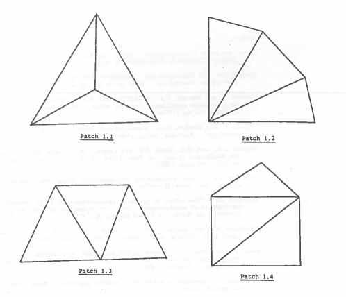
Figure 1: Three-element patches.

To prove patch stability for a class of patches $\boldsymbol{\varepsilon}^{\sigma}_{M}$, we first consider a typical patch $M\in\boldsymbol{\varepsilon}^{\sigma}_{M}$. For this patch we define

(i) $$V^{h}_{M} =\{v\in(H^{1}_{0}(M))^{2}\mid v_{i}\in P_{2}(\triangle)\text{ for }i=1,2\text{ and }\forall\,\triangle\in M\},$$ (10)

(ii) $$P^{h}_{M} =\{p\mid p=p_{0}+p_{1},\ p_{0}\in P_{0}(\triangle)\ \forall\,\triangle\in M,\ p_{1}\in C(\overline{M}),\ p_{1}\in P_{1}(\triangle)\ \forall\,\triangle\in M\}.$$ (11)

The first step in proving patch stability is to find a subspace $R^{h}_{M}$ of $P^{h}_{M}$ that satisfies the condition

$$\inf_{p\in P^{h}_{M}}\sup_{v\in V^{h}_{M}}\left\{\frac{(\operatorname{div}v,p)_{M}}{|v|_{1,M}\,\|p\|_{L^{2}(M)}}\right\}\geq\beta_{M}>0.$$ (12)

The condition (12) is equivalent to the condition

$$p\in R^{h}_{M},\quad(\operatorname{div}v,p)_{M}=0\quad\forall\,v\in V^{h}_{M}\quad\Longrightarrow\quad p=0.$$ (13)

This condition can be established by looking at the null space of the matrix $B$ defined by

$$v\in V^{h}_{M},\quad p\in P^{h}_{M},\quad(\operatorname{div}v,p)_{M}=\underline{v}^{T}B\underline{p},$$ (14)

where $\underline{v}$ is the vector of nodal coordinates determining the finite element function $v\in V^{h}_{M}$ and $\underline{p}$ is the vector of nodal coordinates determining $p\in P^{h}_{M}$. We will then show that the constraints to produce $R^{h}_{M}$ from $P^{h}_{M}$ annihilate this null space. Such a process will establish (12) for the particular patch $M$ and with the particular definition of $R^{h}_{M}$.

Both of the three-element patches 1.1 and 1.2 are important in subsequent sections of this paper and we will define an $R^{h}_{M}$ and show that the constraints annihilate the null space in both cases.

The patch 1.1

A typical patch of this type, type 1, is illustrated in figure 2. For this patch we define

$$R^{h}_{M}=\{p\mid p\in P^{h}_{M},\ p_{0}\in L^{2}_{0}(M),\ p_{1}\in L^{2}_{0}(M)\}.$$ (15)

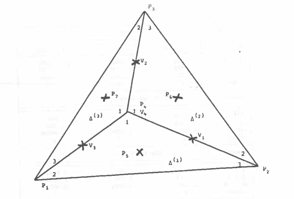
Figure 2: A patch of type 1.

The patch has three elements $(\triangle^{(i)})^{3}_{i=1}$ and we have

$$\underline{v}^{T} =\{(V_{1})_{1},(V_{1})_{2},(V_{2})_{1},(V_{2})_{2},(V_{3})_{1},(V_{3})_{2},(V_{4})_{1},(V_{4})_{2},\},$$

$$\underline{p}^{T} =\{P_{1},P_{2},\dots,P_{7}\},$$

with $B$ an $8\times 7$ matrix. We denote by $|\triangle^{(i)}|$ and $|M|$ the area of $\triangle^{(i)}$ and $M$ respectively and by the two-dimensional vector $b^{(i)}_{j}$ in $\triangle^{(i)}$ the usual values

$$(b^{(i)}_{1})_{1}=y^{(i)}_{2}-y^{(i)}_{3},\quad(b^{(i)}_{1})_{2}=x^{(i)}_{3}-x^{(i)}_{2},\text{ etc.}$$

with the local nodes of each element illustrated in figure 2. The matrix $B$ is given by

$$\frac{1}{6}\begin{bmatrix}-b^{(1)}_{2}&b^{(2)}_{1}+b^{(1)}_{1}&-b^{(2)}_{3}&b^{(2)}_{2}+b^{(1)}_{3}&-4b^{(1)}_{2}&-4b^{(2)}_{3}&0\\[4.0pt] -b^{(3)}_{3}&-b^{(2)}_{2}&b^{(3)}_{1}+b^{(2)}_{1}&b^{(3)}_{2}+b^{(2)}_{3}&0&-4b^{(2)}_{2}&-4b^{(3)}_{3}\\[4.0pt] b^{(1)}_{1}+b^{(3)}_{1}&-b^{(1)}_{3}&-b^{(3)}_{2}&b^{(1)}_{2}+b^{(3)}_{3}&-4b^{(1)}_{3}&0&-4b^{(3)}_{2}\\[4.0pt] 0&0&0&0&-b^{(1)}_{1}&-b^{(2)}_{1}&-b^{(3)}_{1}\end{bmatrix}$$ (16)

and has null space spanned by

$$\begin{split}S^{T}_{1}&=(1,1,1,1,0,0,0),\\ S^{T}_{2}&=(0,0,0,0,1,1,1).\end{split}$$ (17)

We denote by $S$ the $7\times 2$ matrix, the first column of which is $S_{1}$ and the second is $S_{2}$. The constraints that give $R^{h}_{M}$ from $P^{h}_{M}$ are

1. $\int_{M}p_{0}\,d\Omega=0$,

2. $\int_{M}p_{1}\,d\Omega=0$,

which constrain the vector $\underline{p}$ by

1. $P_{5}|\triangle^{(1)}|+P_{6}|\triangle^{(2)}|+P_{7}|\triangle^{(3)}|=0$,

2. $P_{1}(|\triangle^{(1)}|+|\triangle^{(3)}|)+P_{2}(|\triangle^{(2)}|+|\triangle^{(1)}|)+P_{3}(|\triangle^{(3)}|+|\triangle^{(2)}|)+P_{4}|M|=0$,

which we write as

$$H\underline{p}=\underline{0},$$ (18)

where $H$ is a $2\times 7$ matrix. The only vector in the null space of $B$ that satisfies both constraints is the zero vector if the matrix

$$C_{M}=HS$$ (19)

is of full column rank. Here $C_{M}$ is given by

$$\begin{bmatrix}0&|M|\\ 3|M|&0\end{bmatrix}.$$ (20)

Clearly (20) is nonsingular, therefore for any patch $M$ of type 1 with $R^{h}_{M}$ given by (15), the inequality (12) is satisfied provided $R^{h}_{M}$ is nonempty. In section 3 we will construct functions belonging to $R^{h}_{M}$.

The patch 1.2

A typical patch of this type, type 2, is illustrated in figure 3 with $\underline{v}$ a four-dimensional vector and $\underline{p}$ eight dimensional.

Figure 3: A patch of type 2.

The matrix $B$ is the $4\times 8$ matrix

$$\frac{1}{6}\begin{bmatrix}-b^{(1)}_{3}&b^{(2)}_{1}+b^{(1)}_{1}&-b^{(2)}_{2}&0&b^{(2)}_{3}+b^{(1)}_{2}&-4b^{(1)}_{3}&-4b^{(2)}_{2}&0\\[4.0pt] 0&-b^{(2)}_{3}&b^{(3)}_{1}+b^{(2)}_{1}&-b^{(3)}_{2}&b^{(3)}_{3}+b^{(2)}_{2}&0&-4b^{(2)}_{3}&-4b^{(3)}_{2}\end{bmatrix}$$ (21)

which has a null space spanned by

$$\begin{split}S^{T}_{1}&=(1,1,1,1,1,0,0,0),\\ S^{T}_{2}&=(0,0,0,0,0,1,1,1),\\ S^{T}_{3}&=(4,0,0,0,0,-1,0,0),\\ S^{T}_{4}&=(0,0,0,4,0,0,0,-1).\end{split}$$ (22)

Here we note that the matrix $S$ is an $8\times 4$ matrix, the $i$th column of which is $S_{i}$. It is not possible for the two constraints to produce $R^{h}_{M}$ given by (15) to give a matrix $C_{M}$ of full column rank (because with these constraints $C_{M}$ is a $2\times 4$ matrix). Thus we need to apply further constraints on $P^{h}_{M}$ to annihilate the null space. We define $R^{h}_{M}$ by

$$\begin{split}R^{h}_{M}=\{p\mid p\in P^{h}_{M},\ p_{0}\in L^{2}_{0}(M),\ p_{1}\in L^{2}_{0}(M),\\ \qquad\qquad\qquad p\in L^{2}_{0}(\triangle^{(i)})\;\forall\,\triangle^{(i)}\text{ with two sides on the boundary of }&M\}.\end{split}$$ (23)

Thus the constraints are

1. $\int_{M}p_{0}\,d\Omega=0\Longrightarrow P_{6}|\triangle^{(1)}|+P_{7}|\triangle^{(2)}|+P_{8}|\triangle^{(3)}|=0$,

2. $\int_{M}p_{1}\,d\Omega=0\Longrightarrow P_{1}|\triangle^{(1)}|+P_{2}(|\triangle^{(1)}|+|\triangle^{(2)}|)+P_{3}(|\triangle^{(2)}|+|\triangle^{(3)}|)+P_{4}|\triangle^{(3)}|+P_{5}|M|=0$,

3. $\int_{\triangle^{(1)}}p\,d\Omega=0\Longrightarrow P_{1}+P_{2}+P_{5}+3P_{6}=0$,

4. $\int_{\triangle^{(3)}}p\,d\Omega=0\Longrightarrow P_{3}+P_{4}+P_{5}+3P_{8}=0$,

giving us the constraint equation of the form (18). Thus, here,

$$C_{M}=HS=\begin{bmatrix}0&|M|&-|\triangle^{(1)}|&-|\triangle^{(3)}|\\[4.0pt] 3|M|&0&4|\triangle^{(1)}|&4|\triangle^{(3)}|\\[4.0pt] 3&3&1&0\\[4.0pt] 3&3&0&1\end{bmatrix}.$$ (24)

Clearly, (24) is nonsingular, therefore for any patch $M$ of the type 2 with $R^{h}_{M}$ given by (23), the inequality (12) is satisfied provided $R^{h}_{M}$ is nonempty. In section 4 we will construct functions belonging to $R^{h}_{M}$ for this patch.

Stability over classes of topologically equivalent patches

In this section we shall use the important result in Stenberg [10], who observed that, given a class $\boldsymbol{\varepsilon}^{\sigma}_{M}$ of topologically equivalent patches which satisfy (12) for every $M\in\boldsymbol{\varepsilon}^{\sigma}_{M}$, then the value of

$$\beta_{M}=\inf_{p\in R^{h}_{M}}\sup_{v\in V^{h}_{M}}\left\{\frac{(\operatorname{div}v,p)_{M}}{|v|_{1,M}\,\|p\|_{L^{2}(M)}}\right\}$$ (25)

is independent of a transformation of the form

$$\tilde{\underline{x}}=A(\underline{x}-\underline{\alpha}),$$ (26)

where $A$ and $\alpha$ are fixed. This, together with the regularity constraint (6) allows us to represent the whole range of values of $\beta_{M}$ for $M\in\boldsymbol{\varepsilon}^{\sigma}_{M}$ as a function over a compact set $R$, every point of which represents a patch (or indeed many patches) belonging to $\boldsymbol{\varepsilon}^{\sigma}_{M}$. Thus there exists $\beta>0$ such that

$$\beta=\min_{R}(\beta_{M})=\min_{M\in\boldsymbol{\varepsilon}^{\sigma}_{M}}(\beta_{M})$$ (27)

for which

$$\inf_{p\in R^{h}_{M}}\sup_{v\in V^{h}_{M}}\left\{\frac{(\operatorname{div}v,p)_{M}}{|v|_{1,M}\,\|p\|_{L^{2}(M)}}\right\}\geq\beta>0$$ (28)

for every $M\in\boldsymbol{\varepsilon}^{\sigma}_{M}$ with $\beta$ independent of $M$ and $h$ and depending only on the topology of $\boldsymbol{\varepsilon}^{\sigma}_{M}$ and $\sigma$. Thus here, for a given $\sigma$, we have two classes $\boldsymbol{\varepsilon}^{\sigma}_{1}$ and $\boldsymbol{\varepsilon}^{\sigma}_{2}$ of elements topologically equivalent to the patches of type 1, and 2 respectively, and the inequality (28) holds for these two classes with different values of $\beta$. We will actually use an equivalent form of (28), namely for each $p\in R^{h}_{M}$, there exists $v_{M}\in V^{h}_{M}$ such that

$$\begin{split}(\operatorname{div}v_{M},p)_{M}&\geq\beta\|p\|_{L^{2}(M)}^{2},\\[-2.0pt] |v_{M}|_{1,M}&\leq C\|p\|_{L^{2}(M)},\end{split}$$ (29)

or, for $\gamma>0$,

$$\begin{split}(\operatorname{div}(\gamma v_{M}),p)_{M}&\geq\beta\gamma\|p\|_{L^{2}(M)}^{2},\\[-2.0pt] |(\gamma v_{M})|_{1,M}&\leq C\gamma\|p\|_{L^{2}(M)},\end{split}$$ (30)

with $\beta$ and $C$ depending only on the class of patches and on $\sigma$.

Global stability of grids made up of patches of the type 1

In order to use the results of the previous section we construct an operator $\Pi^{(1)}_{M}p$ by

$$\Pi^{(1)}_{M}p =\frac{1}{|M|}\int_{M}p\,d\Omega=k_{0}+k_{1},$$ (31)

$$\text{where}\quad k_{0}=\frac{1}{|M|}\int_{M}{p_{0}}\,d\Omega,\quad k_{1}=\frac{1}{|M|}\int_{M}{p_{1}}\,d\Omega.$$ (32)

Thus, since

$$\int_{M}(p_{0}-k_{0})\,d\Omega=0,\quad\int_{M}(p_{1}-k_{1})\,d\Omega=0$$

then using the argument from Stenberg [10] we can establish the following theorem and corollary.

Theorem 3.1.

For every $p\in P^{h}_{M}$,

1. $p-\Pi^{(1)}_{M}p\in R^{h}_{M}$, $R^{h}_{M}$ defined by (15),

2. $(\operatorname{div}v,\Pi^{(1)}_{M}p)=0\quad\forall\,v\in V^{h}_{M}$.

Corollary (Corollary to Theorem 3.1).

For each $p\in P^{h}_{M}$, there exists $v_{M}\in V^{h}_{M}$ such that

$$\begin{split}\big{(}\operatorname{div}v_{M},p\big{)}_{M}&\geq\beta_{1}\|p-\Pi^{(1)}_{M}p\|_{L^{2}(M)}^{2},\\ |v_{M}|_{1,M}&\leq C_{1}\|p-\Pi^{(1)}_{M}p\|_{L^{2}(M)},\end{split}$$

where $\beta_{1}$ and $C_{1}$ are independent of $p$ and $v_{M}$ but are dependent on $\sigma$.

The proof of global stability on a grid made up of patches of the type 1 now follows that given by Stenberg [10] or Boland & Nicolaides [2]. Moreover, we have the optimal rates of convergence to the solution $(u,q)$ of the Stokes equation, namely

$$|u-u^{h}|_{1,\Omega}+\|q-q^{h}\|_{L^{2}(\Omega)}\leq Ch^{2}(|u|_{3,\Omega}+\|q\|_{2,\Omega})$$ (33)

where $(u^{h},q^{h})$ is the numerical solution in $V^{h}\times P^{h}$.

Further results on the patch of the type 2

Before we establish global stability and optimal rates of convergence, there are further results required for a patch of this type. Let $M$ be a patch of the type 2, we construct an operator $\Pi^{(2)}_{M}$ on the set $P^{h}_{M}$ by

$$\Pi^{(2)}_{M}p=\begin{cases}k^{(2)}\enskip\text{in }\triangle^{(2)},\\ 4k^{(2)}\big{(}1-3L^{(i)}\big{)}-3k^{(i)}\big{(}1-4L^{(i)}\big{)}\enskip\text{in }\triangle^{(1)}\text{ and }\triangle^{(3)},\end{cases}$$ (34)

where

1. $\triangle^{(i)}$ is defined in figure 3,

2. $L^{(i)}$ is the areal coordinate in $\triangle^{(i)}$, $i=1$ and $3$, equal to 1 at the intersection of the two sides on the boundary $\partial M$ of $M$,

3. $$k^{(i)}=\frac{1}{|\triangle^{(i)}|}\int_{\triangle^{(i)}}\!{p\,d\Omega}\quad\text{for }i=1,2,3.$$ (35)

Theorem 4.1.

For every $p\in P^{h}_{M}$ then

1. $$p-\Pi^{(2)}_{M}\mu\in R^{h}_{M},\quad R^{h}_{M}\textup{ defined by \eqref{eq:23}},$$ (36)

2. $$\big{(}\operatorname{div}v,\Pi^{(2)}_{M}p\big{)}_{M}=0\quad\forall\,v\in V^{h}_{M}.$$ (37)

Proof.

(A) Clearly $p=\Pi^{(2)}_{M}p\in P^{h}_{M}$, thus we have to show that $p-\Pi^{(2)}_{M}p$ satisfies the constraints from $P^{h}_{M}$ to $R^{h}_{M}$. We write

$$\left[\Pi^{(2)}_{M}p\right]_{0} =\begin{cases}(1-\alpha)k^{(2)}\enskip\text{in }\triangle^{(2)}\\ (1-\alpha)k^{(2)}+3\big{(}k^{(2)}-k^{(i)}\big{)}\enskip\text{in }\triangle^{(i)},\quad i=1\text{ and }3,\end{cases}$$ (38)

$$\left[\Pi^{(2)}_{M}p\right]_{1} =\begin{cases}\alpha k^{(2)}\enskip\text{in }\triangle^{(2)}\\ \alpha k^{(2)}-12\big{(}k^{(2)}-k^{(i)}\big{)}L^{(i)}\enskip\text{in }\triangle^{(i)},\quad i=1\text{ and }3,\end{cases}$$ (39)

with

$$\alpha=\frac{\int_{M}p_{1}\,d\Omega+4(k^{(2)}-k^{(1)})|\triangle^{(1)}|+4(k^{(2)}-k^{(3)})|\triangle^{(3)}|}{k^{(2)}|M|}$$ (40)

if $k^{(2)}\neq 0$. (If $k^{(2)}=0$ then the definition of $\big{[}\Pi^{(2)}_{M}p\big{]}_{i}$ for $i=0,1$ is independent of $\alpha$.)

We now observe that

$$\int_{M}p_{0}-\left[\Pi^{(2)}_{M}p\right]_{0}\,d\Omega=0, \int_{M}p_{1}-\left[\Pi^{(2)}_{M}p\right]_{1}\,d\Omega=0,$$

$$\int_{\triangle^{(1)}}p-\Pi^{(2)}_{M}p\,d\Omega=0, \int_{\triangle^{(3)}}p-\Pi^{(2)}_{M}p\,d\Omega=0.$$

Thus we have established part (A).

(B) Taking the left-hand side of (37),

$$\begin{split}\big{(}\operatorname{div}v,\Pi^{(2)}_{M}p\big{)}_{M}&=\big{(}\operatorname{div}v,k^{(2)}\big{)}_{M}+3\big{(}k^{(2)}-k^{(1)}\big{)}\big{(}\operatorname{div}v,(1-4L^{(1)})\big{)}_{\triangle^{(1)}}\\ &\quad+3\big{(}k^{(2)}-k^{(3)}\big{)}\big{(}\operatorname{div}v,(1-4L^{(3)})\big{)}_{\triangle^{(3)}}.\end{split}$$ (41)

The first term in (41) is zero because $v\in V^{h}_{M}$. If $L^{(1)}$ is $L^{(1)}_{3}$ in $\triangle^{(1)}$ then $v=V_{1}(4L^{(1)}_{2}L^{(1)}_{1})$, thus we see immediately that the second term in (41) is zero and so therefore is the third. ∎

Corollary (Corollary to Theorem 4.1).

For each $p\in P^{h}_{M}$ there exists $v_{M}\in V^{h}_{M}$ such that

$$(\operatorname{div}v_{M},p)_{M} \geq\beta_{2}\|p-\mu_{M}\|_{L^{2}(\triangle^{(2)})}^{2}\,,$$ (42)

$$|v_{M}|_{1,M} \leq C_{2}\|p-\mu_{M}\|_{L^{2}(\triangle^{(2)})}\,,$$ (43)

with

$$\mu_{M}=\frac{1}{|\triangle^{(2)}|}\int_{\triangle^{(2)}}p\,d\Omega,$$ (44)

where $\beta_{2}$ and $C_{2}$ depend only on the regularity constant $\sigma$.

Proof.

By Theorem 4.1 and inequalities (30), for each $p\in P^{h}_{M}$ there exists $\tilde{v}_{M}$ such that, for $\gamma>0$,

$$(\operatorname{div}(\gamma\tilde{v}_{M}),p)_{M}=\big{(}\operatorname{div}(\gamma\tilde{v}_{M}),p-\Pi^{(2)}_{M}p\big{)}\geq\beta_{2}\gamma\,\big{\|}p-\Pi^{(2)}_{M}p\big{\|}_{L^{2}(M)}^{2},$$

$$|\gamma\tilde{v}_{M}|_{1,M}\leq c_{2}\gamma\big{\|}p-\Pi^{(2)}_{M}p\big{\|}_{L^{2}(M)}.$$

The result follows by choosing

$$\gamma=\big{\|}p-\Pi^{(2)}_{M}p\big{\|}_{L^{2}(\triangle^{(2)})}\bigg{/}\big{\|}p-\Pi^{(2)}_{M}p\big{\|}_{L^{2}(M)},$$ (45)

noting that $\sigma<\gamma<1$, and choosing $v_{M}=\gamma\tilde{v}_{M}$. ∎

Global stability of grids made up of patches of the type 2

We assume that $\Omega$ is a polygonal region which has been triangulated into $N$ triangular elements $(E^{(i)})$. We further assume that each element $E^{(i)}$ sits inside an extended patch $M_{i}$ of the type 2 as element $\triangle^{(2)}$. Firstly we note that these patches overlap. Secondly we note that this assumption does exclude some grids of triangles, namely those which either

1. contain triangular elements with two sides on the boundary, or

2. contain a patch of the form 1.1 with that patch having a side on the boundary.

We can see this by looking at figure 4, elements $E^{(2)}$ to $E^{(12)}$ all sit as element $\triangle^{(2)}$ of a patch of the type 2 but elements $E^{(1)}$ and $E^{(13)}$ do not.

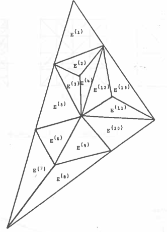
Figure 4: Sample triangulation illustrating the restrictions on the grid.

We consider $\mu\in L^{2}_{0}(\Omega)$ such that $\mu$ is constant in each $E^{(i)}$, Girault & Raviart [3] show that for each $\mu$ there exists $\tilde{v}\in V^{h}$ such that

$$\begin{split}(\operatorname{div}\tilde{v},\mu)_{\Omega}&=\|\mu\|_{L^{2}(\Omega)}^{2},\\ |\tilde{v}|_{1,\Omega}&\leq\tilde{c}\|\mu\|_{L^{2}(\Omega)}.\end{split}$$ (46)

Let $p\in P^{h}$, we define $\mu\in L^{2}_{0}(\Omega)$ such that $\mu$ in the element $E^{(i)}$ is the constant value

$$\mu=\frac{1}{|E^{(i)}|}\,\int_{E^{(i)}}p\,d\Omega\quad\text{in }E^{(i)}\text{ for }i=1,\ldots,N;$$ (47)

thus by the corollary to Theorem 4.1, for each $p\in P^{h}$ there exists $v_{M_{i}}\in V^{h}_{M_{i}}$ such that

$$(\operatorname{div}v_{M_{i}},p)_{M_{i}} \geq\beta_{2}\|p-\mu\|_{L^{2}(E^{(i)})}^{2},$$ (48)

$$|v_{M_{i}}|_{1,M_{i}} \leq C_{2}\|p-\mu\|_{L^{2}(E^{(i)})}.$$ (49)

We note that $\beta_{2}$ and $C_{2}$ do not depend on the particular patch $M$ and depend only on the regularity constant $\sigma$. Thus, for each $p\in P^{h}$ there exists $\tilde{v}\in V^{h}$ such that

$$(\operatorname{div}\tilde{v},p)_{\Omega} \geq\tilde{\beta}\|p-\mu\|_{L^{2}(\Omega)}^{2},$$ (50)

$$|\tilde{v}|_{1,\Omega} \leq\tilde{c}\|p-\mu\|_{L^{2}(\Omega)},$$ (51)

where

(a) $$\tilde{v} =\sum^{N}_{i=1}\tilde{v}_{i},$$

(b) $$\tilde{v}_{i} =\begin{cases}v_{M_{i}}&\text{in }M_{i},\\ 0&\text{elsewhere in }\Omega,\end{cases}$$ (52)

(c) $$\tilde{C} =C_{2},\quad\tilde{\beta}=\beta_{2}.$$

Following Stenberg [10] the inequalities (46) and (50) establish that for each $p\in P^{h}$ then

$$v=\tilde{v}+\left(\frac{2\tilde{\beta}}{1+\tilde{C}^{2}}\right)\tilde{v}$$ (53)

satisfies

$$(\operatorname{div}v,p)_{\Omega} \geq\left(\frac{\tilde{\beta}}{1+\tilde{C}^{2}}\right)\|p\|_{L^{2}(\Omega)}^{2},$$ (54)

$$|v|_{1,\Omega} \leq\left(\tilde{C}+\frac{2\tilde{\beta}\tilde{C}}{1+\tilde{C}^{2}}\right)\|p\|_{L^{2}(\Omega)}.$$ (55)

Thus we have global stability and optimal rates of convergence on all grids that satisfy the regularity constraint (6) and restrictions on the triangles mentioned at the beginning of this section.

It is only the former of these restrictions, namely that we must triangulate ‘into the corners’ that is an essential restriction. By including patches of the form 1.1 in the above argument then the second restriction can be removed but now $\tilde{\beta}=\max(\beta_{1},\beta_{2})$ and $\tilde{C}=\min(C_{1},C_{2})$. Thus we have established optimal convergence rates on all grids of triangles provided the grid has been triangulated into the corners. Further discussion of this topic when the grid has not been triangulated into the corners is given in the appendix.

Numerical examples

In this section we shall consider two numerical examples. The first is a simple test problem to demonstrate that optimal convergence rates are achieved and the second is an example where the Taylor–Hood element gives poor results but the linear plus constant pressure element, which we shall call the LC element, gives relatively good results.

Testing rates of convergence

The first test problem is one proposed by Griffiths & Mitchell [6]. It is an enclosed flow problem (namely a Stokes flow) in the unit square with solution

$$\begin{split}v_{x}&=-20xy^{3},\\ v_{y}&=5y^{4}-5x^{4},\\ p&=-60x^{2}y+20y^{3}+5.\end{split}$$ (56)

Typical grids for this test problem are illustrated in figure 5 and the solutions (i.e. norms

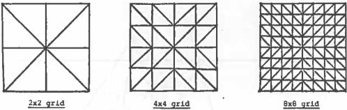
Figure 5: Typical grids for the Griffiths problem.

of the errors) are presented in table 1 with the results for the LC element compared with the Taylor–Hood element and the Raviart bubble element; see Girault & Raviart [4]. It can be seen that the error for the LC and Taylor–Hood elements are comparable and both are much smaller than the Raviart bubble element for this problem. Moreover, for all three elements, the optimal convergence rates are observed.

Table 1: Computed errors for the Griffiths test problem

Grid	$\|p\|_{L^{2}(\Omega)/R}$	$\|\vec{v}\|_{H^{1}(\Omega)}$	$\|\vec{v}\|_{L^{2}(\Omega)}$
	Taylor–Hood element
$4\times 4$	0.4283	0.4802	0.01669
$8\times 8$	0.0975	0.1189	0.00239
$16\times 16$	0.0233	0.0296	0.00029
Order	${\sim}2$	${\sim}2$	${\sim}3$
	LC element
$4\times 4$	0.4878	0.4865	0.01637
$8\times 8$	0.1009	0.1190	0.00237
$16\times 16$	0.0233	0.0296	0.00029
Order	${\sim}2$	${\sim}2$	${\sim}3$
	Raviart bubble element
$4\times 4$	1.5469	0.6834	0.02416
$8\times 8$	0.4314	0.1797	0.00342
$16\times 16$	0.1142	0.0462	0.00043
Order	${\sim}2$	${\sim}2$	${\sim}3$

Illustrating difficulties with the Taylor–Hood element

The solution of a non-Newtonian fluid in the volume of revolution of the region illustrated in figure 6, with the boundary conditions given in the figure, can be reduced to solving the following set of equations

$$\frac{1}{\mathcal{R}}\left(\frac{\partial^{2}V_{r}}{\partial r^{2}}+\frac{\partial^{2}V_{r}}{\partial z^{2}}+\frac{1}{r}\frac{\partial V_{r}}{\partial r}-\frac{V_{r}}{r^{2}}\right)-\frac{\partial p}{\partial r} =-\textup{N}_{\textup{n}}\frac{V^{2}_{\theta}}{r}+\textup{N}_{\textup{e}}\bigg{[}\left(\frac{\partial V_{\theta}}{\partial r}-\frac{V_{\theta}}{r}\right)^{2}+\left(\frac{\partial V_{\theta}}{\partial z}\right)^{2}\bigg{]},$$ (57a)

$$\frac{1}{\mathcal{R}}\left(\frac{\partial^{2}V_{\theta}}{\partial r^{2}}+\frac{\partial^{2}V_{\theta}}{\partial z^{2}}+\frac{1}{r}\frac{\partial V_{\theta}}{\partial r}-\frac{V_{\theta}}{r^{2}}\right) =0,$$ (57b)

$$\frac{1}{\mathcal{R}}\left(\frac{\partial^{2}V_{z}}{\partial r^{2}}+\frac{\partial^{2}V_{z}}{\partial z^{2}}+\frac{1}{r}\frac{\partial V_{z}}{\partial r}\right)-\frac{\partial p}{\partial z} =0,$$ (57c)

$$\frac{\partial V_{r}}{\partial r}+\frac{V_{r}}{r}+\frac{\partial V_{z}}{\partial z} =0,$$ (57d)

after a number of assumptions have been made; further details of which are given by Tidd [12]. For a Newtonian fluid the parameter $\textup{N}_{\textup{e}}=0$ and for a non-Newtonian fluid this parameter gives a measure of the non-Newtonian effects. We note that equation (57b) is independent of $V_{r}$, $V_{z}$, $p$, $\textup{N}_{\textup{e}}$ and decouples from the other three equations whereas equations (57a), (57c), (57d) represent a Stokes flow problem in $(r,z)$ coordinates. This can be solved for the two cases $(\textup{N}_{\textup{n}}=1,\textup{N}_{\textup{e}}=0)$ and $(\textup{N}_{\textup{n}}=0,\textup{N}_{\textup{e}}=1)$ and the particular solution required can be obtained by selecting the required ratio of these two intermediate solutions.

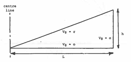
Figure 6: The second test problem $(L=1.0,h=0.1)$.

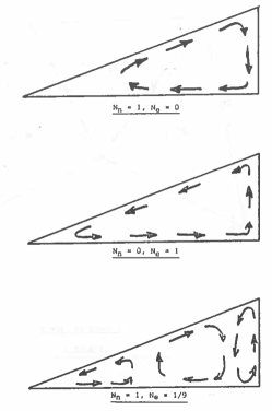
Figure 7: Illustration of the secondary recirculations for the cases of interest $(\mathcal{R}=10)$.

The main flow in this problem is a swirling ($V_{\theta}$) flow with the $V_{r}$ and $V_{z}$ representing secondary flows. An indication of the secondary flows for the three cases

1. $(\textup{N}_{\textup{n}}=1,\textup{N}_{\textup{e}}=0)$,

2. $(\textup{N}_{\textup{n}}=0,\textup{N}_{\textup{e}}=1)$,

3. $(\textup{N}_{\textup{n}}=1,\textup{N}_{\textup{e}}=1/9)$,

is given in figure 7. The three secondary recirculations of (c) have been observed by Hoppmann & Baronet [8] and it is in attempting to model these three recirculations that we find that the Taylor–Hood element gives a very poor solution even on a highly refined grid.

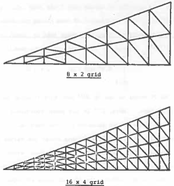
Figure 8: Typical grids for the second test problem.

Typical grids used are illustrated in figure 8. The $V_{\theta}$ problem, namely equation (57b) was solved on each of the grids. On a given grid the relevant $V_{\theta}$ numerical solution was used on the right-hand side of equation (57a).

We find that the Taylor–Hood and LC elements gave essentially the same results for the case $(\textup{N}_{\textup{n}}=1,\textup{N}_{\textup{e}}=0)$ but very different answers for the case $(\textup{N}_{\textup{n}}=0,\textup{N}_{\textup{e}}=1)$ with the LC solutions giving far more consistency from one grid to the next. Moreover, for the case $(\textup{N}_{\textup{n}}=1,\textup{N}_{\textup{e}}=1/9)$, where we are expecting to observe three recirculations, the Taylor–Hood element gives only one complete recirculation with velocities in almost random directions over almost half the region of the problem, namely $0\leq r\leq 0.5$, even on a highly refined $64\times 16$ grid. However, the LC element resolves all three recirculations on a $16\times 4$ grid and gives very good consistency between the $32\times 8$ and $64\times 16$ grids.

We note that the above problem does not fall into the analysis in section 5. Not only is the problem in $(r,z)$ coordinates but also we have not triangulated into all the corners. By modifying the grid so that we do triangulate into all the corners the solutions obtained do not change in any significant way.

In order to obtain a solution with the LC element when we have not triangulated into the corners it is necessary either to fix a pressure in each element with two sides on the boundary or to make the centroid pressure in this element equal to the centroid pressure in the element with a shared side. In fact these two strategies only affect the pressure solution in the element with two sides on the boundary but the analysis of the latter approach is more simple, and is discussed in the appendix.

Conclusion

We have established stability and convergence for the LC element on a wide range of grids. The proof had an interesting feature, namely enclosing the patches under consideration in larger and overlapping extended patches. This idea may prove useful in establishing convergence for other elements for which (div-)stability is difficult to obtain.

When using the element for an enclosed flow problem it is necessary to fix two pressure values, one must be a centroid pressure and the other a vertex pressure.

Finally, the LC element clearly has some interesting features that make it worthy of consideration. In particular the fact that it is locally incompressible has been demonstrated to be useful in practice.

Acknowledgements

We would like to acknowledge the support of the SERC who provided one of us (RWT) with a grant to collaborate with Professor Nicolaides at Pittsburgh, and to Professor Nicolaides for his help in getting the work in this report concluded. We would also like to acknowledge the contribution of David Tidd, an SERC research student, who calculated the numerical results for the second example.

Appendix A Appendix. Restoring stability when the grid is not triangulated into the corners

In this appendix we assume that $\Omega$ has been split up into $N$ elements $(E^{(i)})^{N}_{i=1}$ with the first $n$ of them having two sides on the boundary. A simple numerical experiment shows that we cannot use the element LC for $(E^{(i)})^{N}_{i=1}$ because the continuity equation namely

$$\int_{E^{(i)}}\operatorname{div}v^{h}_{M}\,d\Omega=0,\quad 1\leq i\leq n,$$ (A1)

with $M$ equal to one in $E^{(i)}$ and with $M$ equal to $L^{(i)}$ in $E^{(i)}$ are linearly dependent. (Here, $L^{(i)}$ is the areal coordinate in $E^{(i)}$ equal to $1$ at the vertex between two sides on the boundary $\partial\Omega$ of $\Omega$). We can overcome this difficulty by arbitrarily assigning either the vertex pressure or the centroid pressure (to zero or any other value) without affecting the velocity solution. It is interesting to note that this strategy does not destroy the reason for introducing the element since the equations (A1) with $M$ equal to one or $L^{(i)}$ are merely multiples of each other and keeping either of them in the system of equations ensures continuity over the element $E^{(i)}$. If we make the particular choice of removing the centroid pressure (i.e. setting it to zero), then this is equivalent to using a Taylor–Hood element for $E^{(i)}$, $1\leq i\leq n$. It is surprising that we have not been able to obtain a satisfactory stability result for this strategy.

We could set this centroid pressure to any other value and it only affects the resulting numerical solution by changing the pressure approximation in that element. The particular strategy that we analyse below is choosing the centroid pressure in $E^{(i)}$to be equal to the centroid pressure in $E^{(n+i)}$, where $E^{(n+i)}$ is the element that has a side in common with $E^{(i)}$. This is equivalent to using the pressure space

$$\begin{split}P^{h}=\big{\{}p\mid p&=p_{0}+p_{1};\quad p_{0}\in P_{0}(E^{(i)}\cup E^{(n+i)})\quad\forall\,i=1,\ldots,n,\\ p_{0}&\in P_{0}(E^{(i)})\quad\forall\,i=n+1,\ldots,N;p_{0}\in L^{2}_{0}(\Omega);\\ p_{1}&\in P_{1}(E^{(i)})\quad\forall\,i=1,\ldots,N;\ p_{i}\in L^{2}_{0}(\Omega)\cap C(M)\big{\}}.\end{split}$$ (A2)

Let $M$ be the three-element patch of type 3 illustrated in figure 9 for which

$$\begin{rcases}\triangle^{(1)}=E^{(j)}\\ \triangle^{(2)}=E^{(n+j)}\end{rcases}\quad\text{for }1\leq j\leq n.$$ (A3)

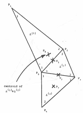
Figure 9: A patch of type 3.

Using the notation of section 2 then $\underline{v}$ is a four-dimensional vector and $\underline{p}$ a seven-dimensional vector and the space $P^{h}_{M}$ for this patch is

$$\begin{split}P^{h}_{M}=\big{\{}p=p_{0}+p_{1}\mid p_{0}\in P^{0}(\triangle^{(1)}\cup\triangle^{(2)}),\ p_{0}\in P_{0}(\triangle^{(3)}),&\\ p_{1}\in C(\overline{M}),\ p_{1}\in P_{1}(\triangle^{(i)})\text{ for }i=1,2,3&\big{\}}.\end{split}$$ (A4)

The matrix $B$ is the $4\times 7$ matrix

$$\begin{bmatrix}-b^{(1)}_{3}&b^{(2)}_{1}+b^{(1)}_{1}&-b^{(2)}_{2}&0&b^{(2)}_{3}+b^{(1)}_{2}&0&0\\[4.0pt] 0&-b^{(2)}_{3}&b^{(3)}_{1}+b^{(2)}_{1}&-b^{(3)}_{2}&b^{(3)}_{3}+b^{(2)}_{2}&-4b^{(2)}_{3}&-4b^{(3)}_{2}\end{bmatrix}$$ (A5)

which has null space spanned by

$$\begin{split}S^{T}_{1}&=(1,1,1,1,1,0,0),\\ S^{T}_{2}&=(0,0,0,0,0,1,1),\\ S^{T}_{3}&=(0,0,0,4,0,0,-1),\end{split}$$ (A6)

and we denote by $S$ the $7\times 3$ matrix the $i$th column of which is $S_{i}$. The space $R^{h}_{M}$ for this patch is defined to be

$$R^{h}_{M}=\big{\{}p\mid p=p_{0}+p_{1}\in P^{h}_{M},\ p_{0}\in L^{2}_{0}(M),\ p_{1}\in L^{2}_{0}(M),\ p\in L^{2}_{0}(\triangle^{(3)})\big{\}}.$$ (A7)

Thus the constraints from $P^{h}_{M}$ to $R^{h}_{M}$ are

1. $\displaystyle\int_{M}p_{0}\,d\Omega=0\Longrightarrow P_{6}\big{(}|\triangle^{(1)}|+|\triangle^{(2)}|\big{)}+P_{7}|\triangle^{(3)}|=0$,

2. $\displaystyle\int_{M}p_{1}\,d\Omega=0\Longrightarrow P_{1}|\triangle^{(1)}|+P_{2}\big{(}|\triangle^{(1)}|+|\triangle^{(2)}|\big{)}+P_{3}\big{(}|\triangle^{(2)}|+|\triangle^{(3)}|\big{)}+P_{4}|\triangle^{(3)}|+P_{5}|M|=0$,

3. $\displaystyle\int_{\triangle^{(3)}}p\,d\Omega=0\Longrightarrow P_{3}+P_{4}+P_{5}+3P_{7}=0$,

giving the constraint equation (23) and the matrix $C_{M}$ is given by

$$C_{M}=HS=\begin{bmatrix}0&|M|&-|\triangle^{(3)}|\\[4.0pt] 3|M|&0&4|\triangle^{(3)}|\\[4.0pt] 3&3&1\end{bmatrix},$$ (A8)

which is clearly nonsingular.

We denote by $\boldsymbol{\varepsilon}^{\sigma}_{3}$ the class of patches of type 3 illustrated in figure 9. Thus, for every $M\in\boldsymbol{\varepsilon}^{\sigma}_{3}$ then for each $p\in R^{h}_{M}$ (defined by (A7)) there exists $v_{M}\in V^{h}_{M}$ (defined by (10)) such that

$$\begin{split}(\operatorname{div}(\alpha v_{M}),p)_{M}&\geq\alpha\beta_{3}\|p\|_{L^{2}(M)}^{2},\\ |\alpha v_{M}|_{1,M}&\leq\alpha C_{3}\|p\|_{L^{2}(M)},\end{split}$$ (A9)

with $\beta_{3}$ and $C_{3}$ independent of the choice of $M\in\boldsymbol{\varepsilon}^{\sigma}_{3}$ but dependent on the regularity constant $\sigma$, where $\alpha$ is any positive constant.

Letting $M\in\boldsymbol{\varepsilon}^{\sigma}_{3}$, we construct an operator $\Pi^{(3)}_{M}$ on the set $P^{h}_{M}$ (defined by (A9)) by

$$\Pi^{(3)}_{M}p=\begin{cases}k=k^{(1)}+k^{(2)}&\text{in }\triangle^{(1)}\text{ and }\triangle^{(2)},\\ 4k\big{(}1-3L^{(3)}\big{)}-3k^{(3)}\big{(}1-4L^{(3)}\big{)}&\text{in }\triangle^{(3)},\end{cases}$$ (A10)

where

1. $\triangle^{(i)}$ are as shown in figure 9,

2. $L^{(3)}$ is the areal coordinate in $\triangle^{(3)}$ that is equal to zero on the side in common with $\triangle^{(2)}$,

3. $k^{(i)}$ is defined as in (35).

Theorem A.1.

For every $p\in P^{h}_{M}$ then

1. $p-\Pi^{(3)}_{M}p\in R^{h}_{M}$,

2. $\big{(}\operatorname{div}v,\Pi^{(3)}_{M}p\big{)}=0\quad\forall\,v\in V^{h}_{M}$

(with $P^{h}_{M}$, $R^{h}_{M}$, $V^{h}_{M}$ defined by (A4), (A7), (10) respectively).

Proof.

To prove (I) we need to show two results. First, that

$$\int_{\triangle^{(3)}}\big{(}p-\Pi^{(3)}_{M}p\big{)}\,d\Omega=0.$$ (A11)

Second, that we can split $\big{(}p-\Pi^{(3)}_{M}p\big{)}$ into

$$\big{(}p-\Pi^{(3)}_{M}p\big{)}=\left[p-\Pi^{(3)}_{M}p\right]_{1}+\left[p-\Pi^{(3)}_{M}p\right]_{0}$$ (A12)

such that

1. $\big{[}p-\Pi^{(3)}_{M}p\big{]}_{0}$ is constant in $\triangle^{(1)}\cup\triangle^{(2)}$, constant in $\triangle^{(3)}$ and satisfies

   $$\int_{M}\left[p-\Pi^{(3)}_{M}p\right]_{0}\,d\Omega=0,$$ (A13)

2. $\big{[}p-\Pi^{(3)}_{M}p\big{]}_{1}$ is linear in each $\triangle^{(i)}$, is continuous over $M$ and satisfies

   $$\int_{M}\left[p-\Pi^{(3)}_{M}p\right]_{1}\,d\Omega=0.$$ (A14)

To do this we write

1. $p=p_{0}+p_{1}$, with $p_{0}$ and $p_{1}$ defined by (A3),

2. $\big{[}p-\Pi^{(3)}_{M}p\big{]}_{1}=\begin{cases}p_{1}-\alpha&\quad\text{in }\triangle^{(1)}\cup\triangle^{(2)}\\ p_{1}-\alpha-12\big{(}k^{(3)}-k\big{)}L^{(3)}&\quad\text{in }\triangle^{(3)},\end{cases}$

3. $\big{[}p-\Pi^{(3)}_{M}p\big{]}_{0}=\begin{cases}p_{0}-k+\alpha&\quad\text{in }\triangle^{(1)}\cup\triangle^{(2)}\\ p_{0}-4k+3k^{(3)}+\alpha&\quad\text{in }\triangle^{(3)},\end{cases}$

with $\alpha$ as yet undefined. Next, choosing $\alpha$ so that

$$\alpha=\frac{k|M|+3\big{(}k-k^{(3)}\big{)}|\triangle^{(3)}|-\int_{M}p_{0}\,d\Omega}{|M|},$$ (A15)

ensures that equation (A13) is satisfied. Moreover, since the definition (A10) of $\Pi^{(3)}_{M}p$ ensures that

$$\int_{M}\big{(}p-\Pi^{(3)}_{M}p\big{)}\,d\Omega=0,$$ (A16)

then, for this value of $\alpha$, we see that equation (A14) is also satisfied. Finally, the definition of $\Pi^{(3)}_{M}p$ ensures that equation (A11) holds. Thus we have established part (I) of the theorem. Part (II) of the theorem follows by the same argument as used in part (B) of theorem 4.1. ∎

Corollary (Corollary to theorem A.1).

For each $p\in P^{h}_{M}$ there exists $v_{M}\in V^{h}_{M}$ such that

$$(\operatorname{div}v_{M},p)_{M} \geq\beta_{3}\|p-\mu_{M}\|_{L^{2}(\triangle^{(1)}\cup\triangle^{(2)})}^{2},$$

$$|v_{M}|_{1,M} \leq c_{3}\|p-\mu_{M}\|_{L^{2}(\triangle^{(1)}\cup\triangle^{(2)})},$$

with

$$\mu_{M}=\frac{\int_{\triangle^{(1)}\cup\triangle^{(2)}}p\,d\Omega}{|\triangle^{(1)}|+|\triangle^{(2)}|}.$$

Proof.

The proof of this corollary is similar to the proof of the corollary to theorem 4.1. ∎

To establish global stability and optimal convergence rates we assume that $\Omega$ is a polygonal region which has been triangulated into $N$ triangular elements $\{E^{(i)}\}^{N}_{i=1}$. We assume that the first $n$ of these elements (with $n\ll N$) have two sides in common with the boundary $\partial\Omega$ of $\Omega$. We denote by $E^{(n+1)}$ that element which has a side in common with $E^{(i)}$, $1\leq i\leq n$, and we denote by $M_{n+1}$ the extended patch of the type 3 which contains $E^{(i)}$ as element $\triangle^{(1)}$ and $E^{(n+i)}$ as element $\triangle^{(2)}$. We further assume that each element $E^{(i)}$, $2n+1\leq i\leq N$, sits inside an extended patch $M_{i}$ of the type 2 as element $\triangle^{(2)}$. These assumptions exclude grids that

1. contain two elements both of which have two sides on the boundary $\partial\Omega$ of $\Omega$ and which have a side in common with a single element of the grid,

2. contain patches of the type 1 with one side in common with boundary $\partial\Omega$ of $\Omega$.

We define the pressure space $P^{h}$ by (A2) and a function $\mu\in L^{2}_{0}(\Omega)$ by

$$\mu=\begin{cases}\int_{E^{(i)}\cup E^{(n+i)}}p\,d\Omega\big{/}{(|E^{(i)}|+|E^{(n+i)}|)}&\quad\text{in }E^{(i)}\cup E^{(n+i)}\quad\text{ for }i=1,2,\dots,n\\[2.0pt] \int_{E^{(i)}}p\,d\Omega\big{/}{|E^{(i)}|}&\quad\text{in }E^{(i)}\quad\text{ for }i=2n+1,\dots,n.\end{cases}$$

The argument now follows that in section 5 recognising that there are two types of patch involved and with

$$\tilde{C}=\max(C_{2},C_{3}),\quad\beta=\min(\beta_{2},\beta_{3}).$$

Thus, we obtain global stability and optimal convergence rates (i.e. inequality (33)) on a wide range of grids even when the grid has not been triangulated into the corners.

To generalise the above argument to include all possible grids in this optimal convergence result we have to reconsider those grids that are excluded. The exclusion (a) above can be overcome by taking a three-element patch that looks like the patch 1.2 or 1.3 in which the term $p_{0}$ is constant throughout the patch. In practice, as one refines the grid to obtain more accurate results the necessity for having such elements as described in (a) is removed.

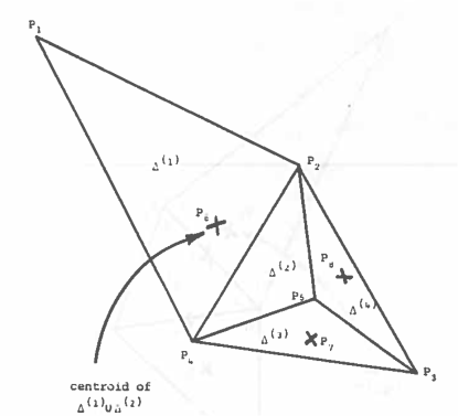
Figure 10: A four-element patch.

The elements excluded by (b) can be included in the argument by using patches of the type 1 as mentioned in section 5. But to fully generalise the argument we need to also include the four-element patch illustrated in figure 10 to cover the hypothetical possibility that for one of the elements $\{E^{(i)}\}^{n}_{i=1}$, the element $E^{(n+i)}$ belongs to a patch of the type 1 which has oneside on the boundary. In this patch the term $p_{0}$ in the pressure space is constant throughout $\triangle^{(1)}\cup\triangle^{(2)}$ (or equivalently $E^{(i)}\cup E^{(n+i)}$).

References

- [1] Bercovier, M. and Pironneau, O. Error estimates for finite element method solution of the Stokes problem in the primitive variables. Numer. Math. 33, 211–224 (1979).
- [2] Boland, J.M. and Nicolaides, R.A. Stability of finite elements under divergence constraints. SIAM J. Numer. Anal. 20, 722–731 (1983).
- [3] Girault, V. and Raviart, P.A. Finite Element Approximation of the Navier–Stokes Equations. Lecture Notes in Mathematics 749, Springer (1979).
- [4] Girault, V. and Raviart, P.A. Finite Element Methods for Navier–Stokes Equations. Springer (1986).
- [5] Gresho, P.M., Lee, R.L., Chan, S.T. and Leone Jr, J.M. A new finite element for incompressible or Boussinesq fluids. In Proc. Third Int. Conf. on Finite Elements in Flow Problems, pp. 204–215 (1981).
- [6] Griffiths, D.F. and Mitchell, A.R. Finite elements for incompressible flow. Math. Meth. Appl. Sci. 1, 16–31 (1979).
- [7] Griffiths, D.F. The effect of pressure approximations on finite element calculations of incompressible flows. In Numerical Methods for Fluid Dynamics (K.W. Morton and M.J. Baines eds) pp. 359–374. Academic Press, San Diego (1982).
- [8] Hoppmann, W.H. and Baronet, C.N. Study of flow induced in viscoelastic liquid by a rotating cone. Trans. Soc. Rheol. 9, 417–423 (1965).
- [9] Hood, P. and Taylor, C. Navier–Stokes equations using mixed interpolation. In Finite Element Methods in Flow Problems, pp. 121–132, Huntsville: UAH Press (1974).
- [10] Stenberg, R. Analysis of mixed finite elements methods for the Stokes problem: a unified approach. Math. Comput. 42, 9–23 (1984).
- [11] Tidd, D.M., Thatcher, R.W. and Kaye, A. The free surface of Newtonian and non-Newtonian fluids trapped by surface tension. NA Report 127 Manchester University/UMIST Joint Series (1986).
- [12] Tidd, D.M. Finite element calculations for flow in rheogoniometers with a free surface. PhD Thesis, UMIST, Manchester, UK (1987).