RENORMALON EFFECTS IN TOP-MASS SENSITIVE OBSERVABLES

Abstract

A precise determination of the top mass is one of the key goals of the LHC and future colliders. Since power corrections are now becoming a source of worry for top-mass measurements, in these proceedings I discuss the impact of linear infrared renormalons, which plague the definition of the top pole-mass $m$, on observables expressed in terms of $m$ and in terms of a short-distance mass.

1 Introduction

The top quark is one of the most peculiar particles predicted by the Standard Model and its phenomenology is entirely driven by the large value of its mass $m_{t}$. The most precise measurements of $m_{t}$ are based on the use of Monte Carlo (MC) event generations and the current errors are of the order of several hundreds of MeV. Thus, linear power corrections arising from the pole mass ambiguity, which is estimated to be of the order of 110-250 MeV[1, 2], are becoming a major worry in top-mass measurements at hadron colliders. Furthermore, even if the perturbative calculations implemented in the MC generators adopt the pole-mass scheme, there is still no consensus in the theoretical community regarding the interpretation of such measurements, due to the complicated interplay of hadronization and parton shower dynamics[3]. The purpose of these proceedings is not to investigate the relation between the pole and the MC mass (see e.g.[4]), but instead to investigate the asymptotic behaviour of quantities calculated in terms of the pole mass and of the $\overline{\rm MS}$ mass (that we can consider as a proxy of all the short-distance mass schemes) in a simplified theoretical frameworks where we understand some aspects concerning the non perturbative corrections to the pole mass. We focus upon the case of single top production and we look at the total cross section, which is known to be free from physical linear renormalons, the reconstructed-top mass, which is highly sensitive to the value of $m_{t}$, and leptonic observables, which are assumed to be independent from non-perturbative QCD effects. More details can be found in Refs.[5, 6].

2 QCD infrared renormalons

In gauge theories in general, and in QCD in particular, there is a certain class of Feynman graphs whose number grows as the factorial of the order of the perturbative expansion in the strong coupling constant. The resulting perturbative series is then divergent and it is typically treated as an asymptotic series. As a consequence, there is an uncertainty in the value of the sum of the series of the order $(\Lambda_{\mathrm{QCD}}/Q)^{p}$, being $Q$ the scale of the process, $\Lambda_{\mathrm{QCD}}$ the infrared scale at which the validity of perturbative QCD breaks down and $p$ a positive integer. This is the so-called renormalon ambiguity[7].

Indeed, when we perform all-orders calculations, some contributions can be thought as NLO corrections where the fixed-scale coupling is replaced with the running one. After the removal of the UV and IR divergencies, the perturbative series will take the form

$$Q^{-p}\int_{0}^{Q}d\ell\,\ell^{p-1}\,\alpha_{s}(\ell)\approx Q^{-p}\sum_{i=0}^{\infty}\alpha_{s}^{n+1}(Q)\int_{0}^{Q}\ell^{p-1}d\ell\left(b_{0}\log\left(\frac{Q^{2}}{\ell^{2}}\right)\right)^{n}=\sum_{i=0}^{\infty}\frac{n!}{p}\left(\frac{2b_{0}}{p}\right)^{n}\alpha_{s}^{n+1}(Q),$$ (1)

where $\ell$ is the (real or virtual) gluon momentum, $p$ is a positive integer and $b_{0}$ is the one-loop QCD $\beta$ function

$$b_{0}=\frac{11C_{A}}{12\pi}-\frac{n_{l}T_{R}}{3\pi},$$ (2)

with $n_{l}$ being the number of light flavours. Since $b_{0}$ is positive, the series in eq. 1 is not even Borel resummable. The terms in the series will first decrease until

$$\frac{n!}{p}\left(\frac{2b_{0}}{p}\right)^{n}\approx\frac{(n+1)!}{p}\left(\frac{2b_{0}}{p}\right)^{n+1}\alpha_{s}(Q)\quad\Rightarrow\quad n\approx\frac{p}{2b_{0}\alpha_{s}(Q)}.$$ (3)

At this point, if we want to interpret the series as an asymptotic one, we need to truncate the expansion and the size of the last term, which is also an indication of the ambiguity in our result, will be of the order $(\Lambda_{\mathrm{QCD}}/Q)^{p}$. The dominant ambiguities are the ones corresponding to $p=1$, i.e. the linear renormalons, and those affect the definition of the pole mass.

Performing all-order calculations is however not possible for any non-trivial gauge theory. To overcome this task, we can imagine that the number of flavours $n_{f}$ is large and the dominant corrections arise from $g\to q\bar{q}$ splittings. Thus, everytime we encounter a gluon line, we replace the free propagator with the dressed one

$$\frac{-ig^{\mu\nu}}{\ell^{2}+i\eta}\to\frac{-ig^{\mu\nu}}{\ell^{2}+i\eta}\times\frac{1}{1+\Pi(\ell^{2}+i\eta,\mu^{2})-\Pi_{\rm ct}},$$ (4)

where $\mu^{2}$ is the renormalization scale, $\Pi$ is the fermionic contribution to the vacuum polarization and $\Pi_{\rm ct}$ is the counterterm we introduce to renormalize the strong coupling. In $D=4-2\epsilon$ dimensions we can write

$$\Pi(\ell^{2}+i\eta,\mu^{2})-\Pi_{\rm ct}=-\alpha_{s}(\mu)\frac{n_{f}T_{R}}{3\pi}\left[\log\frac{|\ell^{2}|}{\mu^{2}}-i\pi\theta(\ell^{2})+C\right]+\mathcal{O(\epsilon)},$$ (5)

where $C$ is a renormalization-scheme dependent constant ($C=-5/3$ in the $\overline{\rm MS}$ scheme). To recover the non-abelian behaviour of QCD, we can imagine that $n_{f}$ is large and negative. At the end of the computation we match the fictitious number of flavours $n_{f}$ with the real number of light flavours $n_{l}$

$$n_{f}\to n_{l}-\frac{11C_{A}}{4}=-\frac{3\pi b_{0}}{T_{R}},$$ (6)

so that the vacuum polarization appearing in the dressed gluon propagator takes the desired form

$$\Pi(\ell^{2}+i\eta,\mu^{2})-\Pi_{\rm ct}=\alpha_{s}(\mu)\,b_{0}\,\left[\log\frac{|\ell^{2}|}{\mu^{2}}-i\pi\theta(\ell^{2})+C\right]+\mathcal{O(\epsilon)}.$$ (7)

This is the so-called large-$b_{0}$ approximation[8, 9].

3 Single-top production at all orders

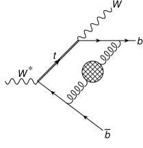
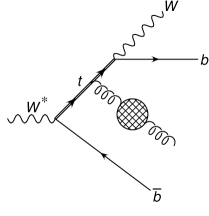
Figure 1: Feynman diagram for Born $W^{*}\to Wb\bar{b}$ process, and samples of Feynman diagrams for the virtual and the real-emission contributions and for the $W^{*}\to Wb\bar{b}q\bar{q}$ production. The bubble denotes the insertion of the vacuum polarization of eq. (7) in the gluon propagator.

We now calculate the process of single-top production and decay, $W^{*}\to t\bar{b}\to Wb\bar{b}$, at all-orders in the large-$b_{0}$ approximation. Explicative examples of the diagrams that must be considered are illustrated in Fig. 1. We stress that together with the virtual and real corrections where the gluon line has been dressed, we also need to include the contribution arising from a real $g\to q\bar{q}$ splitting.

The expression for the total-cross section in presence of selection cuts (that we denote with $\Theta(\Phi)$, being $\Phi$ a phase space point) is given by

$$\sigma=\int d\Phi\frac{d\sigma}{d\Phi}\Theta(\Phi)=\sigma^{(0)}-\frac{1}{\pi b_{0}}\int_{0}^{\infty}d\lambda\frac{d}{d\lambda}\left[\frac{T(\lambda)}{\alpha_{s}(\mu)}\right]\arctan\left[\pi b_{0}\alpha_{s}(\lambda e^{-C/2})\right]$$ (8)

where $\sigma^{(0)}$ is the Born cross section, $C$ is the renormalization-scheme dependent constant that we choose in such a way that

$$\alpha_{s}(\lambda e^{-C/2})=\alpha_{s}(\lambda)+\alpha_{s}^{2}(\lambda)\,b_{0}\,C+\mathcal{O}(\alpha_{s}^{3})\equiv\alpha_{s}(\lambda)+\frac{\alpha_{s}^{2}(\lambda)}{2\pi}\left[\left(\frac{67}{18}-\frac{\pi^{2}}{6}\right)C_{A}-\frac{5}{2}n_{l}\right]=\alpha^{\rm CMW}_{s}(\lambda),$$ (9)

where CMW denotes the Catani-Marchesini-Webber renormalization scheme for the strong coupling[11], also known as the Monte Carlo scheme. The function $T(\lambda)$ is given by

$$T(\lambda)=\sigma^{(1)}(\lambda)+\frac{3\lambda^{2}}{2T_{R}\alpha_{s}(\mu)}\int d\Phi_{g^{*}}d\Phi_{\rm dec}\frac{d\sigma^{(2)}_{q\bar{q}}(\Phi)}{d\Phi}\left[\Theta(\Phi)-\Theta(\Phi_{g^{*}})\right],$$ (10)

where $\sigma^{(1)}(\lambda)$ is the $\mathcal{O}(\alpha_{s})$ cross section calculated with a gluon of mass $\lambda$, $\sigma^{(2)}_{q\bar{q}}$ is the leading-order cross section for the process $W^{*}\to Wb\bar{b}q\bar{q}$, $\Phi_{g^{*}}$ is the phase-space for the production of a heavy gluon of mass $\lambda$, $\Phi_{\rm dec}$ the phase-space for its decay into a $q\bar{q}$ pair (so that the total phase space $\Phi$ can be written as $d\Phi=\frac{d\lambda^{2}}{2\pi}d\Phi_{g^{*}}d\Phi_{\rm dec}$). Thus we see that the factor $T(\lambda)-\sigma^{(1)}(\lambda)$ takes into account the fact that the event in which the $q\bar{q}$ pair has been clustered in a massive gluon $g^{*}$ can lead to different kinematics with respect to the full event. This term is closely related to the Milan factor[10].

It is easy to check that the $\mathcal{O}(\alpha_{s})$ expansion of eq. 8 is given by $\sigma^{(0)}+\sigma^{(1)}(0)$, as expected. From eq. 8 we also see that we have a linear renormalon if

$$\frac{dT(\lambda)}{d\lambda}\Big{|}_{\lambda=0}\neq 0,$$ (11)

so we will focus our attention on the small-$\lambda$ behaviour of the function $T(\lambda)$ to assess the presence of linear renormalons.

4 Results

In this section we present the most relevant phenomenological results of Ref.[5]. The center-of-mass energy is chosen to be $E=300$ GeV, the $W$ mass is set to 80.4 GeV and the bottom mass is set to 0. We choose the complex pole scheme for a consistent treatment of top-offshell effect

$$m^{2}=m^{2}_{0}-im_{0}\Gamma_{t},$$ (12)

where $m_{0}=172.5$ GeV, $\Gamma_{t}=1.3279$ GeV. We choose $m_{0}$ as renormalization scale. We use the $e^{+}e^{-}$ version of the anti-$k_{T}$ algorithm to reconstruct the $b$ and $\bar{b}$ jets. If not specified, we require the $b$ and the $\bar{b}$ jets to be separated and to have a minimum transverse momentum of 25 GeV.

4.1 Cross section

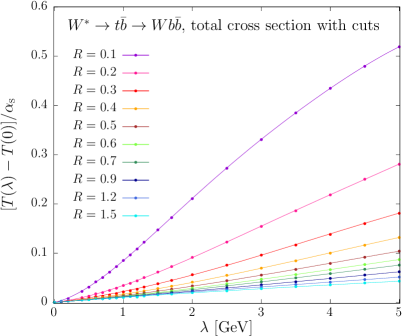
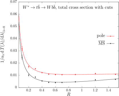
Figure 2: In the left pane the small-$\lambda$ behaviour for $T(\lambda)$ for the total cross section with cuts calculated in the pole scheme for several jet radii. In the right panel the slope of $T(\lambda)$ at $\lambda=0$ for the pole and the $\overline{\rm MS}$ scheme.

For the total cross section without cuts the function $T(\lambda)$ reduces to $\sigma^{(1)}(\lambda)$. For small values of $\lambda$, the linear $\lambda$ term is due to the pole-mass counterterm and is equal to

$$\frac{dT(\lambda)}{d\lambda}\Big{|}_{\lambda=0}=\alpha_{s}(\mu)\frac{C_{F}}{2}\frac{\partial\sigma^{(0)}(m,m^{*})}{\partial{\rm Re}(m)},$$ (13)

where ${\rm Re}(m)$ denotes the real part of the top mass. By expanding eq. (8) in series of $\alpha_{s}(\mu)$, we find that the minimal term is reached at the $8^{\rm th}$ order and leads an ambiguity of relative order $5\times 10^{-4}$.

When the $\overline{\rm MS}$ scheme is employed, such linear renormalon disappears and the behaviour of the perturbative series improves, no visible minimum arises considering the first $10^{\rm th}$ orders and the relative corrections are smaller then $10^{\rm-5}$ already from the $4^{\rm th}$ order.

However, when selections cuts to identify the final state are introduced, the benefit of using the $\overline{\rm MS}$ scheme is reduced. The requirement that the $b$ and the $\bar{b}$ jets are separated and have a minumum transverse momentum of 25 GeV introduces a linear term whose magnitude grows with the inverse of the jet radius, as was found in other contexts as well[12, 13]. This behaviour is illustrated in Fig 2.

4.2 Reconstructed-top mass

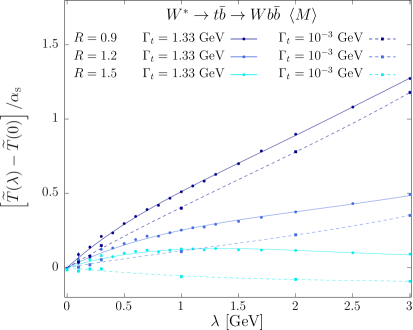
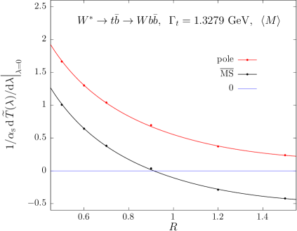
Figure 3: In the left pane the small-$\lambda$ behaviour for $T(\lambda)$ for the reconstructed-top mass calculated in the pole scheme for several jet radii using $\Gamma_{t}=1.3279$ GeV (solid lines) and $\Gamma_{t}=10^{-3}$ GeV (dashed lines). In the right panel the slope of $T(\lambda)$ at $\lambda=0$ for the pole and the $\overline{\rm MS}$ scheme.

We define the reconstructed-top mass $M$ as the mass of the system comprising the final-state $W$ boson and the $b$-jet. As for the case of the cross section, selection cuts introduce a linear-$\lambda$ term in the function $T(\lambda)$, whose magnitude is proportional to the inverse of the jet radius.

For vanishing top width, $M$ approaches the pole mass when a large jet radius is adopted, thus reducing the renormalon ambuiguity. On the other hand, the use of a short distance scheme like the $\overline{\rm MS}$ would introduce a term of the form

$$\frac{1}{\alpha_{s}(\mu)}\frac{dT(\lambda)}{d\lambda}\Big{|}_{\lambda=0}=-\frac{C_{F}}{2}\frac{\partial M(m,m^{*})}{\partial{\rm Re}(m)}\approx-\frac{C_{F}}{2}=-0.667,$$ (14)

and thus have a worse perturbative expansion. This behaviour is due to the fact that this observable contains a physical renormalon that cancels with the pole renormalon if the pole scheme is adopted.

The inclusion of finite-width effects slightly modifies the slope of the function $T(\lambda)$ in the range $\lambda<\Gamma_{t}$, as can be seen from the left panel of Fig. 3. In the right panel of the same figure we see that for large jet radii there is still a large cancellation between the physical renormalon present in the definition of $M$ and the one in the pole mass. In the $\overline{\rm MS}$ scheme we do observe a cancellation between the jet renormalon and the one in $M$ for jet radii of the order of 0.9. However, conversely to the previous case, this cancellation is accidental and cannot be taken as indication of a small overall ambiguity as the two effects should be considered independent source of errors.

4.3 Leptonic observables

The last observable we consider is the average value of the energy of the final-state $W$ boson, $\langle E_{W}\rangle$, which can be considered as a proxy of all leptonic observables. For this analysis we do not impose any selection cuts to avoid to be contaminated by jet renormalons.

We find that in the narrow-width approximation, $\langle E_{W}\rangle$ has a linear renormalon both in the pole and in the ${\rm\overline{MS}}$ scheme. Conversely to the case of the total cross section, if we compute $E_{W}$ in the laboratory frame the calculation cannot be factorized between production and decay, thus spoiling the cancellation of the linear $\lambda$ term in $\langle E_{W}\rangle$. This cancellation takes place only if $E_{W}$ is computed in the top frame.

When a finite width is employed, the top can never be on-shell as $p_{t}^{2}$ is real, thus a linear $\lambda$ term can develop only if the pole mass counterterm is used. However, this is also telling us that we can start appreciating the good convergence of the ${\rm\overline{MS}}$ scheme at orders $n=1+\log(m/\Gamma_{t})\approx 6$, as it can be seen from Tab. 1.

	$\displaystyle\langle E_{W}\rangle$    [GeV]
	—pole scheme —		${\overline{\rm MS}}$ scheme
$\phantom{\Big{|}}i\phantom{\Big{|}}$	$c_{i}$	$c_{i}\,\alpha_{s}^{i}$	$c_{i}$	$c_{i}\,\alpha_{s}^{i}$
1	$-1.435\,(0)\times 10^{1}$	$-1.552\,(0)\times 10^{0}$	$-7.192\,(0)\times 10^{0}$	$-7.779\,(0)\times 10^{-1}$
2	$-4.97\,(4)\times 10^{1}$	$-5.82\,(4)\times 10^{-1}$	$-3.88\,(4)\times 10^{1}$	$-4.54\,(4)\times 10^{-1}$
3	$-1.79\,(5)\times 10^{2}$	$-2.26\,(6)\times 10^{-1}$	$-1.45\,(5)\times 10^{2}$	$-1.84\,(6)\times 10^{-1}$
4	$-6.9\,(4)\times 10^{2}$	$-9.4\,(6)\times 10^{-2}$	$-5.7\,(4)\times 10^{2}$	$-7.8\,(6)\times 10^{-2}$
5	$-2.9\,(3)\times 10^{3}$	$-4.4\,(5)\times 10^{-2}$	$-2.4\,(3)\times 10^{3}$	$-3.5\,(5)\times 10^{-2}$
6	$-1.4\,(3)\times 10^{4}$	$-2.2\,(4)\times 10^{-2}$	$-1.0\,(3)\times 10^{4}$	$-1.7\,(4)\times 10^{-2}$
7	$-8\,(2)\times 10^{4}$	$-1.3\,(4)\times 10^{-2}$	$-5\,(2)\times 10^{4}$	$-8\,(4)\times 10^{-3}$
8	$-5\,(2)\times 10^{5}$	$-9\,(4)\times 10^{-3}$	$-2\,(2)\times 10^{5}$	$-4\,(4)\times 10^{-3}$
9	$-3\,(2)\times 10^{6}$	$-7\,(4)\times 10^{-3}$	$-1\,(2)\times 10^{6}$	$-2\,(4)\times 10^{-3}$
10	$-3\,(2)\times 10^{7}$	$-6\,(5)\times 10^{-3}$	$0\,(2)\times 10^{6}$	$-1\,(5)\times 10^{-4}$

Table 1: Coefficients of the perturbative expansion of the average $W$-boson energy in the pole and $\overline{\rm MS}$-mass schemes.

The last undesirable feature connected to the use of this observable is the reduced sensitivity to the top mass. Indeed, for our choice of the center-of-mass energy $d\langle E_{W}\rangle/dm\approx 0.1$, while in the top frame $d\langle E_{W}\rangle/dm\approx 0.4$.

5 Conclusions

In these proceedings we have summarized the method introduced in Ref.[5] to evaluate all-orders corrections in the large-$b_{0}$ approximation. When the method is applied to processes involving a decaying top quark, we can predict which observables are affected by linear renormalons if the pole or a short-distance mass scheme is adopted. This method is also sensitive to linear corrections associated with jets.

The total cross section does not display linear renormalons related to the top mass if a short distance scheme is adopted. This is the case for leptonic observables only if a finite width $\Gamma_{t}$ is employed, unless such observables are computed in the top frame. This also implies that the good convergence of leptonic-observables predictions will manifest only at high orders ($n\geq 1+\log(m/\Gamma_{t})\approx 6$). The reconstructed-top mass is affected by a physical renormalon that partially cancels with the one contained in the pole mass definition. This cancellation is almost exact for $\Gamma_{t}\to 0$ if the jet radius is large enough.

6 Acknowledgements

The work summarized here has been carried out in collaboration with Paolo Nason and Carlo Oleari. I also want to thank the organisers of LFC19 for the invitation, particularly Gennaro Corcella, Giancarlo Ferrera and Francesco Tramontano, the STRONG-2020 network for the financial support and Tomáš Ježo for useful comments on the manuscript.

References

- 1 . M. Beneke, P. Marquard, P. Nason and M. Steinhauser, Phys. Lett. B 775 (2017) 63 doi:10.1016/j.physletb.2017.10.054 [arXiv:1605.03609 [hep-ph]].
- 2 . A. H. Hoang, C. Lepenik and M. Preisser, JHEP 1709 (2017) 099 doi:10.1007/JHEP09(2017)099 [arXiv:1706.08526 [hep-ph]].
- 3 . M. Butenschoen, B. Dehnadi, A. H. Hoang, V. Mateu, M. Preisser and I. W. Stewart, Phys. Rev. Lett. 117 (2016) no.23, 232001 doi:10.1103/PhysRevLett.117.232001 [arXiv:1608.01318 [hep-ph]].
- 4 . A. H. Hoang, S. Plätzer and D. Samitz, JHEP 1810 (2018) 200 doi:10.1007/JHEP10(2018)200 [arXiv:1807.06617 [hep-ph]].
- 5 . S. Ferrario Ravasio, P. Nason and C. Oleari, JHEP 1901 (2019) 203 doi:10.1007/JHEP01(2019)203 [arXiv:1810.10931 [hep-ph]].
- 6 . S. Ferrario Ravasio, arXiv:1902.05035 [hep-ph].
- 7 . M. Beneke, Phys. Rept. 317 (1999) 1 doi:10.1016/S0370-1573(98)00130-6 [hep-ph/9807443].
- 8 . M. Beneke and V. M. Braun, Phys. Lett. B 348 (1995) 513 doi:10.1016/0370-2693(95)00184-M [hep-ph/9411229].
- 9 . P. Ball, M. Beneke and V. M. Braun, Nucl. Phys. B 452 (1995) 563 doi:10.1016/0550-3213(95)00392-6 [hep-ph/9502300].
- 10 . Y. L. Dokshitzer, A. Lucenti, G. Marchesini and G. P. Salam, Nucl. Phys. B 511 (1998) 396 Erratum: [Nucl. Phys. B 593 (2001) 729] doi:10.1016/S0550-3213(97)00650-0, 10.1016/S0550-3213(00)00646-5 [hep-ph/9707532].
- 11 . S. Catani, B. R. Webber and G. Marchesini, Nucl. Phys. B 349 (1991) 635. doi:10.1016/0550-3213(91)90390-J
- 12 . G. P. Korchemsky and G. F. Sterman, Nucl. Phys. B 437 (1995) 415 doi:10.1016/0550-3213(94)00006-Z [hep-ph/9411211].
- 13 . M. Dasgupta, L. Magnea and G. P. Salam, JHEP 0802 (2008) 055 doi:10.1088/1126-6708/2008/02/055 [arXiv:0712.3014 [hep-ph]].