Complete Solution of the Tight Binding Model on a Cayley Tree: Strongly Localised versus Extended States

Abstract

The complete set of Eigenstates and Eigenvalues of the nearest neighbour tight binding model on a Cayley tree with branching number $b=2$ and $M$ branching generations with open boundary conditions is derived. We find that of the $N=1+3(2^{M}-1)$ total states only $3M+1$ states are extended throughout the Cayley tree. The remaining $N-(3M+1)$ states are found to be strongly localised states with finite amplitudes on only a subset of sites. In particular, there are, for $M>1$, $3\times 2^{M-2}$ surface states which are each antisymmetric combinations of only two sites on the surface of the Cayley tree and have energy eactly at $E=0$, the middle of the band. The ground state and the first two excited states of the Cayley tree are found to be extended states with amplitudes on all sites of the Cayley tree, for all $M$. We use the results on the complete set of Eigenstates and Eigenvalues to derive the total density of states and a local density of states.

I Introduction

Arthur Cayley introduced the Cayley tree graph as a graphical representation of the free groupCayley1878 . The Cayley tree is a tree graph with $N$ nodes, branching number $b$ with degree $k=b+1$, except at surface edge nodes where $k=1$. Since it is loop free, the dynamics on Cayley trees is amenable to exact solutions employing the transfer matrix method. The local density of states at the central site of a tight binding model on a Cayley tree has been derived analytically in Refs. Brinkmann1970 ; Chen1974 ; mahan ; Eckstein2005 ; giacometti . The tight binding model for disordered fermions has been solved analytically by the transfer matrix method on a Cayley tree, revealing the Anderson delocalization transition for $b>1$Beeby1973 ; AbouChacra1973 ; Zirnbauer1986 ; Mirlin1994 . For infinite number of lattice sites the Caylee tree is called Bethe lattice since Bethe’ s approximation for the Ising model becomes exact on this latticeBaxter1982 . The density of states for the Bethe lattice has been derived in Ref. Derrida1993 . Other interacting models, in particular the Hubbard model have been studied on the Bethe lattice. Since in the limit of $k\rightarrow\infty$ mean field theory for any model with interactions becomes exact, the formulation on the Bethe lattice has been used to study this limit in a controlled wayGeorges1996 . The problem of quasiparticle relaxation in an interacting electron system has been mapped on the localization problem in Fock space and solved approximately by mapping it on a Cayley treeAltshuler1997 . Recently, the dynamics of coupled oscillators have been studied on a Cayley tree, as a model for the dynamics in distribution power grids Tamrakar2018 .

Inspite of this wide range of applications of the Cayley tree in physics, the Eigenstates and Energy Eigenvalues of the tight binding model have hardly been studied. In 2001, Mahan obtained the shell symmetric Eigenstates on a Bethe lattice and derived from it the local density of states at the central site. However, the full basis of Eigenstates on a Cayley tree was not obtained there. We therefore intend to fill this gap in this paper by giving the analytical derivation for branching number $b=2$. The numerical analysis of this problem has recently been presented in Ref. Yorikawa2018 .

II The Tight Binding Model on a Cayley Tree

The tight binding model is defined by

$$\hat{H}=\sum_{<i,j>}t_{ij}\ket{i}\bra{j}.$$ (1)

where $t_{ij}$ is the hopping amplitude between sites $i$ and $j$. $<i,j>$ denotes nearest neighbours on the graph. Here $\ket{i}$ denotes the state in which a single particle occupies the site labeled by $i$. We will assume homogenous hopping amplitude $t_{ij}=t,$ in the following (in particular, we set $t=1$ for simplicity). We are interested in obtaining the full set of Eigenstates $\ket{\Psi_{n}}$ with Eigenvalues $E_{n}$ as given by

$$\hat{H}\ket{\Psi_{n}}=E_{n}\ket{\Psi_{n}},$$ (2)

for all $n=1,...,N$, where $N$ is the number of states. Here, we consider the sites to be on a Cayley tree of branching number $b=2$, as shown in Fig. 1 for the example of $M=3$ branching generations, when starting from the central site. The number of sites $N$ is related to the number of branching generations $M$. Noting that each generation $l$ has $3\times 2^{l-1}$ sites, $N=1+3\times\sum_{l=1}^{M}2^{l-1}=1+3(2^{M}-1)$.

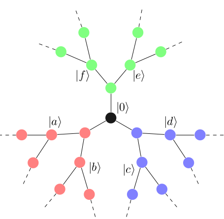
Figure 1: Cayley tree with branching $b=2$ and $M=3$ generations. Its three branches are highlighted by different color.

III Exact Solution

III.1 Choice of basis

Mahan found a subset of $M+1$ Eigenstates of all $N$ Eigenstates on a Cayley tree mahan by using the shell symmetric states as a subbasis for the Eigenstates. These shell symmetric basis states are symmetric with respect to a rotation between different branches of the Cayley tree, which are highlighted by different colors in Fig. 1. The Eigenstates have therefore equal amplitude on all sites of the same generation $l$. Accordingly, we can label these symmetric states with one number that denotes the generation $l$ of the hopping starting from the central site, e.g. $\ket{l=3}$ denotes the symmetric state on all $3^{rd}$ generation sites. Eq. (2) then furnishes recurrence relations. These were solved by Mahan to obtain solutions with equal amplitude on sites of same generation (symmetric solutions)mahan .

In order to obtain all Eigenstates, we need to extend the basis to all states to be able to distinguish between the different branches of the Cayley tree. In a first step, let us split the tree into three main branches starting at the central site as highlighted by different colors in Fig. 1. We denote with $\ket{l}_{m}$ the normalized symmetric combination of local states defined on the nodes of the $l^{th}$ generation in branch $m$, where $l=0$ denotes the central node of the Cayley tree. We enumerate the three branches originating from the $l=0$ site with $m\in\{1,2,3\}$.

For example in Fig. 1

$$\begin{split}\ket{2}_{1}=\frac{1}{\sqrt{2}}(\ket{a}+\ket{b})\\ \ket{2}_{2}=\frac{1}{\sqrt{2}}(\ket{c}+\ket{d})\\ \ket{2}_{3}=\frac{1}{\sqrt{2}}(\ket{e}+\ket{f})\end{split}.$$ (3)

Note that there thus in total $3M+1$ such symmetric basis states $\ket{l}_{m}$, which are orthogonal to each other.

In order to get the remaining basis states, we include successively all antisymmetric superpositions of site states which branch from a node $\alpha$ in the $l^{th}$ generation of the Cayley tree to the right and left as shown in Fig. 2. The basis states are then taken to be the antisymmetric combination of states in the left and right branches evolving from node $\alpha$, as highlighted by red and blue color in Fig. 2 (for each generation). Since there are $3\times 2^{l-1}$ states in each generation $l$, we enumerate these states with $\alpha\in\{1,2,...,3\times 2^{l-1}\}$. Such a state starting in generation $l$ is thus denoted as $\ket{l,r}_{\alpha}$ with $r\in\{1,..,M-l\}$.
For example, for the sites shown in Fig.2 (assuming that $\alpha$ is some node in $l^{th}$ generation of the cayley tree), the state labeled as $\ket{l,r=1}_{\alpha}$, $\ket{l,r=2}_{\alpha}$ and $\ket{l,r=3}_{\alpha}$ are given by

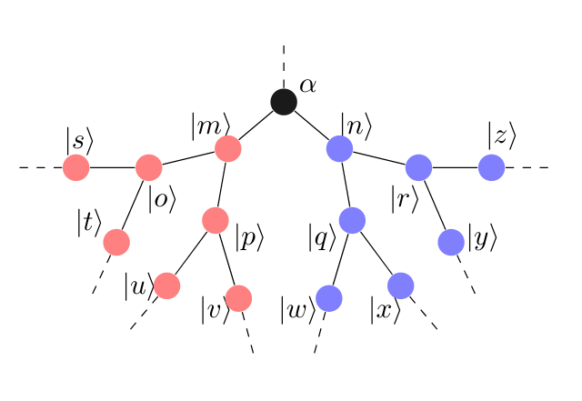
Figure 2: Two branches highlighted by blue and red, arising from node $\alpha$. Forming antisymmetric combinations of all sites on these two branches gives basis states.

$$\ket{l,1}_{\alpha} =\frac{1}{\sqrt{2}}(\ket{m}-\ket{n})$$ (4)

$$\ket{l,2}_{\alpha} =\frac{1}{\sqrt{4}}(\ket{o}+\ket{p}-\ket{q}-\ket{r})$$

$$\ket{l,3}_{\alpha} =\frac{1}{\sqrt{8}}(\ket{s}+\ket{t}+\ket{u}+\ket{v}-\ket{w}-\ket{x}-\ket{y}-\ket{z})$$

and so on for the further generations. Thus, for each node $\alpha$ in the $l^{th}$ generation we get $M-l$ such child states $\ket{l,r}_{\alpha}$, with $r\in\{1,..,M-l\}$. Since there are $3\times 2^{l-1}$ nodes $\alpha$ in the $l^{th}$ generation, the total number of such states is,

$$\begin{split}\sum_{l=1}^{M-1}{3\times 2^{l-1}\left(M-l\right)}=3\left(2^{M}-1\right)-3M=N-1-3M.\end{split}$$ (5)

Together with $3M+1$ symmetric basis states, we get in total $N$ basis states. Note that all antisymmetric states are orthogonal to one another and also to the symmetric states. One way of seeing this is as follows: a symmetric state always has equal amplitude on all nodes of a given branch, whereas an antisymmetric state always has equal number of nodes having positive and negative amplitudes (and can only have non-zero amplitude on nodes of one and the same branch). Thus, this completes the $N$ basis states forming an orthonormal basis for the Hilbert Space of the tight binding model on the Cayley tree with $N$ sites. Using this basis simplifies the solution of the eigenvalue equation Eq. (2), since it can be arranged in blocks, as we will see in the following section.

III.2 Block Recurrence Relations

Any eigenstate $\ket{\Psi}$ can now be written as a superposition of the basis states

$$\begin{split}\ket{\Psi}&=\psi_{0}\ket{0}+\sum_{l=1}^{M}\sum_{m=1}^{3}\psi_{l,m}\ket{l}_{m}\\ &+\sum_{l=1}^{M-1}\sum_{r=1}^{M-l}\sum_{\alpha\in\mathbb{G}_{l}}\phi^{\alpha}_{l,r}\ket{l,r}_{\alpha},\end{split}$$ (6)

where $\psi_{0},\ \phi^{\alpha}_{l,r}\text{ and }\psi_{l,m}$ are complex amplitudes and $\mathbb{G}_{l}$ denotes the set of all $3\times 2^{l-1}$ sites in the $l^{th}$ generation of the Cayley tree.

Insertion of Eq. (6) into the Eigenvalue equation Eq. (2) results then in the following recurrence relations

$$\begin{split}E\psi_{0}&=\psi_{1,1}+\psi_{1,2}+\psi_{1,3},\\ E\psi_{l,m}&=\sqrt{2}(\psi_{l-1,m}+{\psi}_{l+1,m})\\ E{\psi}_{M,m}&=\sqrt{2}{\psi}_{M-1,m},\end{split}$$ (7)

for $l=1,...,M-1$ and $m=1,2,3$, and

$$\begin{split}E{\phi^{\alpha}_{l,1}}&=\sqrt{2}{\phi^{\alpha}_{l,2}},\\ E{\phi^{\alpha}_{l,r}}&=\sqrt{2}({\phi^{\alpha}_{l,r-1}}+{\phi^{\alpha}_{l,r+1}})\\ E{\phi^{\alpha}_{l,M-l}}&=\sqrt{2}{\phi^{\alpha}_{l,M-l-1}}\end{split}$$ (8)

for $l=1,2...,M-1$ and $r=2,...,M-l-1$.

III.3 Solutions of the recurrence relations

Let us start with solutions which satisfy $\psi_{0}=0$, with which Eq. (7) yields,

$$\psi_{1,1}+\psi_{1,2}+\psi_{1,3}=0,$$ (9)

and

$${\psi}_{l,m}=\left(\frac{E^{2}}{2}-1\right){\psi}_{l-2,m}-\frac{E}{\sqrt{2}}{\psi}_{l-3,m},$$ (10)

for $l=1,...,M.$ This gives,

$$\begin{split}{\psi}_{l,m}&=\frac{-2^{\frac{1-3l}{2}}\left(\left(E-\sqrt{E^{2}-8}\right)^{l}-\left(\sqrt{E^{2}-8}+E\right)^{l}\right)}{\sqrt{E^{2}-8}}{\psi}_{1,m}\\ &\equiv k_{l}{\psi}_{1,m},\end{split}$$ (11)

for $l=1,...,M-1$. With the Ansatz for the Energy Eigenvalues $E=2\sqrt{2}\cos\theta$, we get that

$$k_{l}=\frac{1}{(2\sqrt{2})^{l-1}}\frac{\sin{l\theta}}{\sin\theta}.$$ (12)

For now, $\psi_{1,m}$ can be freely choosen provided Eq. 9 is satisfied. This will be fixed later on by requiring that the wavefunction be normalized. The equations in Eq. (7) are closed by the open boundary condition at the surface of the Cayley tree. Open boundary condictions are implemented in the tight binding model by adding another generation of sites $M+1$, where the vanishing of the wave function is imposed

$$\begin{split}{\psi}_{M+1,m}&=0.\\ \end{split}$$ (13)

We note that ${\psi_{1,m}}\neq{0}$ for at least one $m\in\{1,2,3\}$. Eq. (13) requires together with Eq. (11) the quantisation condition

$$\begin{split}k_{M+1}=0~{}\text{or}~{}\frac{\sin\{(M+1)\theta\}}{\sin{\theta}}=0.\end{split}$$ (14)

Thus, we get the following discrete solutions for $\theta$

$$\begin{split}\theta_{i}=\frac{\pi}{M+1}i,\end{split}$$ (15)

with $i\in\{1,2,...,M\}$.
This gives the discrete energy eigenvalues

$$E_{i}=2\sqrt{2}\cos\theta_{i}=2\sqrt{2}\cos\left(\frac{\pi}{M+1}i\right).$$ (16)

Next, we get $\psi_{1,m}$ by imposing the normalization condition

$$\sum_{l=1}^{M}\sum_{m=1}^{3}\absolutevalue{\psi_{l,m}}^{2}=1,$$ (17)

which with Eq. (11) gives,

$$\begin{split}\sum_{l=1}^{N}\sum_{m=1}^{3}k_{l}^{2}\absolutevalue{\psi_{1,m}}^{2}=1\\ \text{or, }\sum_{m=1}^{3}\absolutevalue{\psi_{1,m}}^{2}=\frac{1}{\sum_{l}k_{l}^{2}}.\end{split}$$ (18)

We can eliminate $\psi_{1,3}$ with Eq. (9) to get,

$$\absolutevalue{\psi_{1,1}}^{2}+\absolutevalue{\psi_{1,2}}^{2}+\text{Re}(\psi_{1,1}\psi_{1,2}^{*})=\frac{1}{2\sum_{l}{k_{l}^{2}}}.$$ (19)

Defining $\psi_{1,1}:=r_{1}e^{i\nu_{1}}$ and $\psi_{1,2}:=r_{1}e^{i\nu_{2}}$ we get

$$r_{1}^{2}+r_{2}^{2}+r_{1}r_{2}\cos{(\nu_{1}-\nu_{2})}=\frac{1}{2\sum_{l}{k_{l}^{2}}},$$ (20)

which, for fixed energy $E$, gives a parameter family of ellipses for different $\Delta\nu:=\nu_{1}-\nu_{2}$. For fixed energy $E$ we find the two orthogonal solutions to Eq. 19

$$\begin{split}\psi_{1,1}&=0,\ \psi_{1,2}=\frac{e^{i\mu}}{\sqrt{2}\sqrt{\sum_{l}{k_{l}^{2}}}}\\ \text{and }\psi_{1,1}&=\frac{e^{i\delta}}{\sqrt{2}\sqrt{\sum_{l}{k_{l}^{2}}}},\ \psi_{1,2}=0,\end{split}$$ (21)

for arbitrary phases $\mu$ and $\delta$. Thus, all other solutions of Eq. 19 are linear combinations of these solutions. Next, using Eq. 11 and Eq. 9, we get all remaining complex amplitudes $\psi_{l,m}$.

Thus, for each possible energy eigenvalue $E_{i}$, given by Eq. (16), we get two degenerate orthogonal eigenstates with the following amplitudes on the basis vector components

$$\begin{split}\psi_{1,3}&=-\psi_{1,1}-\psi_{1,2}\\ \text{and }\psi_{l,m}&=k_{l}\psi_{1,m}\\ &=\frac{1}{(2\sqrt{2})^{l-1}}\frac{\sin{(l\theta_{i})}}{\sin\theta_{i}}\psi_{1,m},\end{split}$$ (22)

where the two possible choices of $\psi_{1,1}$ and $\psi_{1,2}$, as given by Eq. (21), give two orthogonal eigenstates with the same energy $E_{i}$. Since there are $M$ possible values of $\theta_{i}$, Eq. (15) and each Eigenspace is two fold degenerate, the total number of states of this kind is $2M$.

The Eigenstates given by Eq. (22) are orthogonal to Mahan’s symmetric solutions, since the basis states in Mahan’s analysis have equal weight in all three branches, and thus $\psi_{l,1}=\psi_{l,2}=\psi_{l,3}$ for all $l$. Since there are $M+1$ Mahan’s solutions and they are orthogonal to the $2M$ solutions obtained above in Eq. (22), we have obtained all the solutions we can get from the subset of $3M+1$ basis states obtained from Eq. 7. We re-do the Mahan’s analysis here. Solving Eq. (7) with the condition that $\psi_{l,1}=\psi_{l,2}=\psi_{l,3}$, we get that

$$\begin{split}\psi_{0,m}&=C\sin\gamma\\ \psi_{l,m}&=C\sin(l\theta+\gamma)\end{split}$$ (23)

where $E=2\sqrt{2}\cos\theta$ and $\gamma$ is related to $\theta$ as:

$$\tan\gamma=3\tan\theta$$ (24)

$C$ is an overall normalization constant. The open boundary condition is imposed by adding another generation of sites and imposing that the wave function vanishes there, $\psi_{M+1,m}=0$. This yields the quantization condition on $0<\theta\leq\pi$ as

$$\sin\{(M+1)\theta+\gamma\}=0,$$ (25)

or

$$\sin\{(M+1)\theta+\tan^{-1}(3\tan\theta)\}=0$$ (26)

This quantization condition, Eq. (26), has $M+1$ solutions with $0<\theta\leq\pi$, which can be found analytically for given $M$.

Having solved the first set of recursion equations Eq. (7), we move on to solve the remaining Eq. (8). For given integer $l$ and $\alpha\in\mathbb{G}_{l}$, the second block of equations in Eq. (8) resembles the set of equations one obtains for the Eigenstates of a tight binding Hamliltonian on an one-dimensional chain with $M-l$ sites. Thereby, we can readily write its solutions as

$$\begin{split}\phi^{\alpha}_{l,r}=&\sqrt{\frac{2}{M-l+1}}\sin{(r\chi)},\end{split}$$ (27)

where $r=1,...,M-l$. The energy eigenvalues are

$$E=2\sqrt{2}\cos{\chi}.$$ (28)

The possible values of $\chi$, for each choice of $l$ and $\alpha$, is obtained from the open boundary conditions $\phi_{M+1,r}^{\alpha}=0$, yielding the quantisation condition

$$\begin{split}\chi_{i}=\frac{\pi}{M-l+1}i\text{~{}for~{} }i={1,2,...,M-l}.\end{split}$$ (29)

In particular, we obtain the surface states for $l=M-1$, where we get

$$\begin{split}\phi^{\alpha}_{M-1,r=1}=\sin{(\chi)}.\end{split}$$ (30)

Eq. (29) dictates that $\chi=\frac{\pi}{2},$ and thus the Eigen energy of the surface states is $E=0$ with eigenstates given by

$$\ket{\Psi}_{\alpha}=\ket{M-1,1}_{\alpha},$$ (31)

which is the antisymmetric combination of the two surface sites branching off from one of the $3\times 2^{M-2}$ sites $\alpha\in\mathbb{G}_{l=M-1}$. Thus, we showed that antisymmetric combination of two surface sites form the surface eigenstates of the Hamiltonian with zero energy, $E=0$. The existence of such zero energy eigenstates can easily be verified directly from the form of the hamiltonian: taking two surface states which are connected to the same site, one verifies that the structure of the Hamiltonian implies that their antisymmetric state is a zero-energy eigenvector of $H$.

One of them is shown in Fig. 3. For a Cayley tree with $M$-generations, there are thus $N_{\rm Surface}=3\times 2^{M-2}$ such surface Eigenstates, which corresponds for $M\gg 1$ to half of the total states, $N_{\rm Surface}|_{M\gg 1}\rightarrow N/4$.

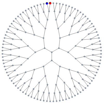
Figure 3: Visualisation of a surface state, strongly localised with non-zero and equal intensity on two sites, only. Red and blue indicate opposite signs of the surface state amplitude.

Having found all Eigenstates of the tight binding Hamiltonian Eq. (1), let us list them in the following.

I. The $M+1$ symmetric states found by Mahan mahan with energy $E^{I}=2\sqrt{2}\cos\theta_{i},$ $i=0,1,...,M$ are given by

$$\ket{\Psi}=\psi_{0}\ket{0}+\sum_{l=1}^{M}\sum_{m=1}^{3}\psi_{l,m}\ket{l}_{m}$$ (32)

$${\rm with~{}}\psi_{0}=C\sin{\gamma_{i}}{\rm~{},~{}}\psi_{l,m}=C\sin({l\theta_{i}+\gamma_{i}}),$$ (33)

where the $M+1$ solutions $0<\theta_{i}\leq\pi$ are obtained from the condition Eq. (26) and the $\gamma_{i}$ is defined by Eq. (24). These states are extended, have equal amplitudes in nodes of the same generation and have finite amplitude $\psi_{0}$ at the centre of the tree. The type I state of lowest energy is obtained by setting the argument of $\sin$ in the condition Eq. (26) equal to $M\pi$, yielding the energy to be $E^{I}_{0}=2\sqrt{2}\cos\theta_{0}$ with $\theta_{0}$ being a solution of the equation

$$\theta_{0}=\frac{M}{M+1}\pi-\frac{1}{M+1}\tan^{-1}(3\tan\theta)).$$ (34)

We find that $\frac{M}{M+1}\pi<\theta_{0}<\pi$, for all $M>1$, since $\tan^{-1}(3\tan\theta)<0$ for $\pi/2<\theta_{0}<\pi$, and the solution $\theta_{0}=\pi$ corresponds to the trivial solution with wavefunction $\psi=0$ which is not an Eigenstate. Thus, we find that the Eigen energy $E^{I}_{0}=2\sqrt{2}\cos\theta_{0}$ is the smallest Eigen energy of all states, including the other type II and type III states and we can conclude that the ground state is for any $M$ the extended symmetric type I state with energy

$$E^{I}_{0}=2\sqrt{2}\cos\theta_{0},$$ (35)

where $\theta_{0}$ is the nontrivial solution of Eq. (34). The ground state for a $M=6$ Cayley tree is shown in Fig. 4.

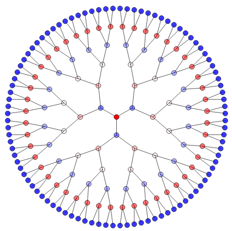
Figure 4: Visualisation of the amplitudes of a type I state for $M=6$ tree. The darkness of the color is proportional to the absolute value of the Eigenstate amplitude. Red denotes positive and blue denotes negative amplitude. Note that the amplitude on sites of the same generation is equal.

II. Next, there are $2M$ states with energies $E^{II}_{i}=2\sqrt{2}\cos\theta_{i}=2\sqrt{2}\cos{\left(\frac{\pi}{M+1}i\right)}$, where $i\in\{1,2..,M\}$, given by

$$\ket{\Psi_{i}}=\sum_{l=1}^{M}\sum_{m=1}^{3}\psi_{l,m}\ket{l}_{m}$$ (36)

with $\psi_{1,3}=-\psi_{1,1}-\psi_{1,2}$, and $\psi_{l,m}=\frac{1}{(2\sqrt{2})^{l-1}}\frac{\sin{l\theta_{i}}}{\sin\theta_{i}}\psi_{1,m}\\$ where each energy $E^{II}_{i}$ is two fold degenerate with two orthogonal states given by $(\psi_{1,1},\psi_{1,2})$ from Eq. (21). These $2M$ states are extended throughout the Cayley tree, except that they have zero amplitude at the centre of the tree. An example is shown in Fig. 5. We note that the type II states with lowest energy are the two states with $i=M$ yielding the energy $E^{II}_{M}=2\sqrt{2}\cos{\left(\frac{\pi}{M+1}M\right)}$.

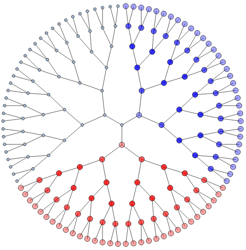
Figure 5: Visualisation of the amplitudes of a Type II state with $\psi_{1,1}=0$. The darkness of the color is proportional to the absolute value of the Eigenstate amplitude. Red denotes positive and blue denotes negative amplitude. Note that the central site has zero amplitude and the amplitude on sites of the same generation on each branch is equal.

III. The remaining states with energeis $E^{III}_{i}=2\sqrt{2}\cos\chi_{i}=2\sqrt{2}\cos{\left(\frac{\pi}{M-l+1}i\right)}$ with $i\in\{1,2,...,M-l\}$ and $l\in\{1,2,...,M-1\}$ are given by

$$\ket{\Psi}_{l,\alpha}=\sum_{r=1}^{M-l}\phi^{\alpha}_{l,r}\ket{l,r}_{\alpha},$$ (37)

with

$$\phi^{\alpha}_{l,r}=\sqrt{\frac{2}{M-l+1}}\sin{(r\chi_{i})},$$ (38)

where $l\in\{1,2,...,M-1\}$ and $\alpha\in\mathbb{G}_{l}$ and $r=1,...,M-l$. For fixed $l$ and $\alpha$, there are thus $M-l$ possible values of $E_{i}=2\sqrt{2}\cos\chi_{i}$ with $\chi_{i}=\frac{\pi}{M-l+1}i$ for $i={1,2,...,M-l}$. Since there are $M$ possible values of $l$ and there are $3\times 2^{l-1}$ nodes $\alpha$ in $\mathbb{G}_{l}$, by similar computation as in Eq. (5), we get that there are $N-(3M+1)$ states of this type. These states are localized to branches of the Caley tree and for increasing $l$ they get more and more localized, with finite amplitude only on $2^{M-l}$ sites. An example of a Type III state for $l=3$ and $M=6$ is shown in Fig. 6. The $3\times 2^{M-2}$ surface states are antisymmetric combinations of two sites with Eigenergy $E=0$, exactly. The type III state with lowest energy is obatined for $l=1$ and $i=M-1$ yielding the energy

$$E^{III}_{l=1,i=M-1}=2\sqrt{2}\cos{\left(\frac{\pi}{M}(M-1)\right)},$$ (39)

which is always larger than energy $E^{I}_{0}$ of the extended ground state and energy $E^{II}_{M}$ of the first excited, extended states.

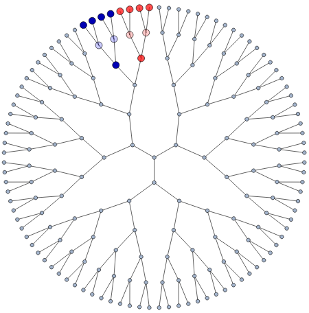
Figure 6: Visualisation of the amplitudes of a Type III state for $l=3$ and $M=6$. The darkness of the color is proportional to the absolute value of the Eigenstate amplitude. Red denotes positive and blue denotes negative amplitude. Note that the amplitude on sites of the same generation is equal.

We note that these results are in complete agreement with the numerical results of Ref. Yorikawa2018 , where numerical results for $M=4$ have been presented. We also note that one can distinguish states with energy $E=2\sqrt{2}\cos\theta$ with $\theta$ being a rational fraction of $\pi$, and others where $\theta$ is an irrational fraction of $\pi$. But we find that this classification is not sufficient to distinguish the different nature of the Eigenstates as we have classified and identified them: The extended type II states and the localised type III states have both an energy $E=2\sqrt{2}\cos\theta$ where $\theta$ is a rational fraction of $\pi$. The type I states can have $\theta$ being an irrational fraction of $\pi$, but may also be a rational fraction of $\pi$. Thus, this irriationality is not a necessary condition for a type I state.

IV Density of States

Mahan had calculated in Ref. mahan, the local density of states at the central site $\rho_{00}(E)$. Since only the $M+1$ shell symmetric states have a finite amplitude $\psi_{0}$ at that site one findsmahan

$$\rho_{00}(E)=\sum_{\theta_{n}}|\psi_{0}(\theta_{n})|^{2}\delta(E-\epsilon_{n}),$$ (40)

where $\epsilon_{n}=2\sqrt{2}\cos{\theta_{n}}$. The summation can be approximated by an integral over $\theta$ in the limit of a Bethe lattice, $M\rightarrow\infty$, where one findsmahan

$$\rho_{00}(E)=\int_{0}^{\pi}d\theta\frac{2}{\pi}{\sin}^{2}(\beta(\theta))\delta(E-\epsilon_{n})=\frac{3}{2\pi}\frac{\sqrt{8-E^{2}}}{9-E^{2}}.$$ (41)

Having obtained all the eigenstates and energies of the Schroedinger equation on the Cayley tree, we can now proceed to calculate the total density of states, given by

$$\rho(E)=\sum_{n}\delta(E-\epsilon_{n})$$ (42)

where the sum is over all Eigen energies $\epsilon_{n}$. It is convenient to write it as a sum of contributions from the threee different different kind of states $I,II,III$, we have derived above,

$$\rho(E)=\rho_{I}(E)+\rho_{II}(E)+\rho_{III}(E)$$ (43)

where $\rho_{I}$ denotes the contribution due to the $M+1$ symmetric Mahan states, $\rho_{II}$ the contribution due to the $2M$ states which have same amplitude in each of the three branches and $\rho_{III}$ the contribution due to the $N-(3M+1)$ states which are localised in different branches of the Cayley tree. In the large $M$ limit, we get

$$\rho_{I}(E)=\frac{M+1}{\pi\sqrt{8-E^{2}}},$$ (44)

see the Appendix for the derivation. Similarly, we find

$$\begin{split}\rho_{II}(E)=\frac{2(M+1)}{\pi\sqrt{8-E^{2}}},\end{split}$$ (45)

and

$$\begin{split}\rho_{III}(E)=\sum_{l=1}^{M-1}\mathbb{D}_{l}\sum_{i=1}^{M-l}\ \delta\left\{E-2\sqrt{2}\cos\left(\frac{\pi}{M-l+1}i\right)\right\},\end{split}$$ (46)

where $\mathbb{D}_{l}=\sum_{\alpha\in\mathbb{G}_{l}}$ = $3\times 2^{l-1}$ is the number of sites in the $l^{th}$ generation. We observe that the degeneracy of the states increases with $M$ as $\sim 2^{M}$ for the $III-$type Eigenstates which are localized near the surface. Thus, in the $M\rightarrow\infty$ limit, those states are highly degenerate.

As an example we show the results for a numerical computation of the density of states for a Cayley tree with $M=3$ generations. We see the distribution of energy eigenvalues and their degeneracies in Fig. 7, in particular that the states at zero energy $E=0$ are highly degenerate. The histogram is symmetric about $E=0$, with same number of states with energy $-E$ as with energy $E$ as is clear from the analytical solution Eqs. 15, 26, 29 for $M=3$.

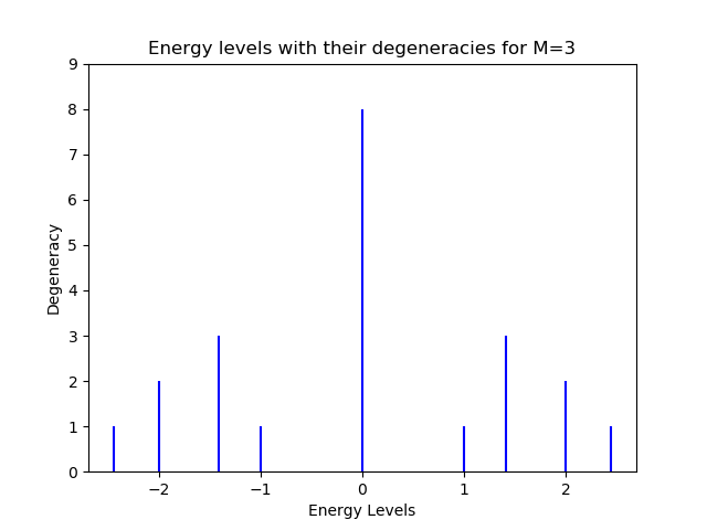
Figure 7: Histogram shows the degeneracy of energy levels computed numerically for $M=3$.

V Conclusion

The complete set of Eigenstates and Eigenvalues of the nearest neighbour tight binding model on a Cayley tree with branching number $b=2$ and $M$ branching generations with open boundary conditions has been derived. Besides the $M+1$ shell symmetric Eigenstates derived already by Mahan in Ref. mahan, , we find $2M$ Eigenstates which have zero amplitude at central site but are otherwise extended throughout the Cayley tree. The remaining $N-(3M+1)$ states are found to be strongly localised states with finite amplitudes on only a subset of sites. In particular, there are $3\times 2^{M-2}$ states which are each antisymmetric combinations of two sites at the surface of the Cayley tree. Thus for $N\gg 1$, there are $N_{\rm surface}\rightarrow N/4$ surface states. We find that the ground state of the Cayley tree is always an extended symmetric state with ground state energy given by Eq. (35). The two first excited states are also extended states. The localised states are spread over the spectrum. The most strongly localised states have energy $E=0$ and are localised on a pair of neighboured surface states, being an antisymmetric superposition of them. The localised states with the largest localisation length of order $M$ sites have the lowest energy of all localised states, given by Eq. (39).

These results are used to derive the total density of states as function of energy $E$. Having all Eigenstates and Eigenfunctions one can now derive the local density of states not only at the central site as in Ref. mahan, but at any site and any one particle observable on the Cayley tree, as well as one particle response functions. Using a similar strategy, choosing a convenient basis, we can derive the Eigenstates for any branching number $b>2,$ a task we leave for a future publication.

After submission of this manuscript, we were made aware of Ref. Yorikawa2018 who studied the same problem, and derived the Eigenstates and Eigenvalues of the Cayley tree numerically, with results which are in agreement with our analytical solutions, as presented here.

Appendix A

Derivation of $\rho_{I}(E).$ With the dispersion relation

$$E_{n}=2\sqrt{2}\cos{\theta_{n}},$$

and the quantization condition

$$\theta_{n}+\frac{\gamma(\theta_{n})}{M+1} =\frac{\pi n}{M+1},$$

we obtain, using $\displaystyle{\sin^{2}{\gamma}=\frac{9\sin^{2}{\theta}}{9-8\cos^{2}{\theta}}}$, the phase differences

$$\theta_{n+1}-\theta_{n}=\frac{\pi}{M+1}-\frac{\gamma(\theta_{n+1})-\gamma(\theta_{n})}{M+1}.$$ (47)

Thus, for $M\rightarrow\infty$ we can approximate the ratio of differences of $\gamma$ and $\theta$ by the first derivative of $\gamma$ with respect to $\theta$,

$$\frac{\gamma(\theta_{n+1})-\gamma(\theta_{n})}{\theta_{n+1}-\theta_{n}}\approx\frac{\partial\gamma(\theta)}{\partial\theta}.$$

Now, writing $x=\sin\theta$ and $y=\sin\gamma$ we obtain $y^{2}=9x^{2}/(1+8x^{2})$ which implies

$$\frac{\partial y}{\partial x}=\frac{3}{(1+8x^{2})^{3/2}}.$$

Thus,

$$\frac{\partial y}{\partial x}=\frac{\partial\sin{\gamma}}{\partial\sin{\theta}}=\frac{\cos{\gamma}}{\cos{\theta}}\ \frac{\partial\gamma}{\partial\theta},$$

and

$$\frac{\partial\gamma}{\partial\theta}=\frac{\cos{\theta}}{\cos{\gamma}}\ \frac{\partial y}{\partial x}=\frac{\cos{\theta}}{\cos{\gamma}}\ \frac{3}{(1+8\sin^{2}{\theta})^{3/2}}.$$

Thereby, Eq. 47 becomes for $M\gg 1$,

$$\theta_{n+1}-\theta_{n} =\frac{\pi}{M+1}-\frac{\gamma(\theta_{n+1})-\gamma(\theta_{n})}{\theta_{n+1}-\theta_{n}}\ \frac{\theta_{n+1}-\theta_{n}}{M+1}$$

$$\approx\frac{\pi}{M+1}\left\{1-\frac{3}{M+1}\frac{\cos{\theta_{n}}}{\cos{\gamma_{n}}}\frac{1}{(1+8\sin^{2}{\theta_{n}})^{3/2}}\right\}$$

$$+\text{o}\left(\frac{1}{(M+1)^{3}}\right).$$

For $M\gg 1$, we thus find with $\theta_{n+1}-\theta_{n}\to\frac{\pi}{M+1}$ that the contribution of the $I-$ states to the density of states is given by

$$\rho_{I}(E) =\frac{M+1}{\pi}\int_{0}^{\pi}d\theta\ \delta(E-2\sqrt{2}\cos\theta)$$

$$=\frac{M+1}{\pi}\int_{\varepsilon(0)}^{\varepsilon(\pi)}d\varepsilon\ \frac{1}{\left|\frac{d\varepsilon}{d\theta}\right|}\delta(E-\varepsilon).$$

With

$$\frac{d\varepsilon}{d\theta}=2\sqrt{2}\sin\theta=2\sqrt{2}\sqrt{1-\cos^{2}\theta}=2\sqrt{2}\sqrt{1-\frac{\varepsilon^{2}}{8}},$$

we finally find

$$\rho_{I}(E)=\frac{M+1}{\pi\sqrt{8-E^{2}}}.$$ (48)

Derivation of $\rho_{II}$. With the dispersion relation $E=2\sqrt{2}\cos(\theta_{i})$ and the quantisation condition $\theta_{i}=\frac{\pi}{M+1}i.$ we find for $M\gg 1$ in the continuum limit and noting that each energy level is 2-fold degenerate,

$$\rho_{II}(E)=\frac{2(M+1)}{\pi\sqrt{8-E^{2}}},$$ (49)

twice the contribution as for the shell symmetric $I-$ states.

Derivation of $\rho_{III}$. With the dispersion relation $E_{i,l}=2\sqrt{2}\cos\left({\frac{\pi}{M-l+1}}i\right)$ for $i=1,2,....,M-l$ and $l=1,2,...,M-1$ we find

$$\rho_{III}(E) =\sum_{l=1}^{M-1}\sum_{\alpha\in\mathbb{G}_{l}}\sum_{i=1}^{M-l}\delta\left\{E-2\sqrt{2}\cos\left(\frac{\pi}{M-l+1}i\right)\right\}$$

$$=\sum_{l=1}^{M-1}\mathbb{D}_{l}\sum_{i=1}^{M-l}\ \delta\left\{E-2\sqrt{2}\cos\left(\frac{\pi}{M-l+1}i\right)\right\}$$

where $\mathbb{D}_{l}=\sum_{\alpha\in\mathbb{G}_{l}}$ is the number of sites in the $l^{th}$ generation, $\mathbb{D}_{l}=3\times 2^{l-1}$.

References

- (1) A. Cayley, ”Desiderata and suggestions: No. 2. The Theory of groups: graphical representation”, American Journal of Mathematics 2, 1 (1878).
- (2) W. F. Brinkman and T. M. Rice, Phys. Rev. B 2, 1324 (1970).
- (3) M. Chen, L. Onsager, J. Bonner, and J. Nagle, J. Chem. Phys. 60, 405 (1974).
- (4) B. Derrida and G. J. Rodgers J. Phys. A: Math. Gen. 26, L457 (1993).
- (5) Mahan, G.D. Energy bands of the Bethe lattice. Phys. Rev. B 63(15), 155110 (2001).
- (6) A. Giacometti, J. Phys. A: Math Gen. 28, L13-L17 (1995).
- (7) M. Eckstein, M. Kollar, K. Byczuk, D. Vollhardt, Phys. Rev. B 71, 235119 (2005).
- (8) J. L. Beeby, J. Phys. C 6, L283 (1973).
- (9) R. Abou-Chacra, D. J. Thouless, and P. W. Anderson, J. Phys. C: Solid State Phys. 6, 1734 (1973); R. Abou- Chacra, and D. J. Thouless, J. Phys. C: Solid State Phys. 7, 65 (1974).
- (10) M. R. Zirnbauer, Phys. Rev. B 34, 6394 (1986).
- (11) A. D. Mirlin and Y. V. Fyodorov, Nucl. Phys B 366, 507 (1991); Phys. Rev. Lett. 72, 526 (1994); J. Phys. (France) 4, 655 (1994).
- (12) R. J. Baxter, Exactly solved models in statistical mechanics, (Academic, London, 1982).
- (13) A. Georges, G. Kotliar, W. Krauth, and M. J. Rozenberg, Rev. Mod. Phys. 68, 13 (1996).
- (14) Boris L. Altshuler, Yuval Gefen, Alex Kamenev, and Leonid S. Levitov, Phys. Rev. Lett. 78, 2803 (1997).
- (15) S. R. Tamrakar, M. Conrath, S. Kettemann, Propagation of Disturbances in AC Electricity Grids, Scientific Reports 8, 6459 (2018).
- (16) H. Yorikawa, J. Phys. Commun. 2, 125009 (2018).