Inverse Filtering for Hidden Markov Models with
Applications to Counter-Adversarial Autonomous Systems

Abstract

Bayesian filtering deals with computing the posterior distribution of the state of a stochastic dynamic system given noisy observations. In this paper, motivated by applications in counter-adversarial systems, we consider the following inverse filtering problem: Given a sequence of posterior distributions from a Bayesian filter, what can be inferred about the transition kernel of the state, the observation likelihoods of the sensor and the measured observations? For finite-state Markov chains observed in noise (hidden Markov models), we show that a least-squares fit for estimating the parameters and observations amounts to a combinatorial optimization problem with non-convex objective. Instead, by exploiting the algebraic structure of the corresponding Bayesian filter, we propose an algorithm based on convex optimization for reconstructing the transition kernel, the observation likelihoods and the observations. We discuss and derive conditions for identifiability. As an application of our results, we illustrate the design of counter-adversarial systems: By observing the actions of an autonomous enemy, we estimate the accuracy of its sensors and the observations it has received. The proposed algorithms are evaluated in numerical examples.

I Introduction

In a partially observed stochastic dynamic system, the state is hidden in the sense that it can only be observed in noise via a sensor. Formally, with $p$ denoting a probability density (or mass) function, such a system is represented by the conditional densities:

$$x_{k} \sim P_{x_{k-1},x}=p(x|x_{k-1}),\quad x_{0}\sim\pi_{0},$$ (1)

$$y_{k} \sim B_{x_{k},y}=p(y|x_{k}),$$ (2)

where by $\sim$ we mean “distributed according to” and $k$ denotes discrete time. In (1), the state $x_{k}$ evolves according to a Markovian transition kernel $P$ on state-space $\mathcal{X}$, and $\pi_{0}$ is its initial distribution. In (2), an observation $y_{k}$ (in observation-space $\mathcal{Y}$) of the state is measured at each time instant according to observation likelihoods $B$. An important example of (1)-(2), where (1) is a finite-state Markov chain, is the so called hidden Markov model (HMM) [1, 2].

In the Bayesian (stochastic) filtering problem [3], one seeks to compute the conditional expectation of the state given noisy observations by evaluating a recursive expression for the posterior distribution of the state:

$$\pi_{k}(x)=p(x_{k}=x|y_{1},\dots,y_{k}),\qquad x\in\mathcal{X}.$$ (3)

The recursion for the posterior is given by the Bayesian filter

$$\pi_{k}=T(\pi_{k-1},y_{k};P,B),$$ (4)

where

$$\{T(\pi,y;P,B)\}(x)=\frac{B_{x,y}\int_{\mathcal{X}}P_{\zeta,x}\pi(\zeta)d\zeta}{\int_{\mathcal{X}}B_{x,y}\int_{\mathcal{X}}P_{\zeta,x}\pi(\zeta)d\zeta dx},\quad x\in\mathcal{X},$$ (5)

– see, e.g., [2, 1] for derivations and details. Two well known finite dimensional cases of (5) are the Kalman filter, where the dynamical system (1)-(2) is a linear Gaussian state-space model, and the HMM filter, where the state is a finite-state Markov chain.

In this paper, we treat and provide solutions to the following inverse filtering problem:

Given a sequence of posteriors $\pi_{1},\dots,\pi_{N}$ from the filter (4), reconstruct (estimate) the filter’s parameters: the system’s transition kernel $P$, the sensor’s observation likelihoods $B$ and the measured observations $y_{1},\dots,y_{N}$.

An important motivating application is the design of counter-adversarial systems[4, 5, 6]: Given measurements of the actions of a sophisticated autonomous adversary, how to remotely calibrate (i.e., estimate) its sensors and predict, so as to guard against, its future actions? We refer the reader to Fig. 1 on the next page for a schematic overview.

This paper extends our recent work [7, 5, 6] in two important ways: First, [7, 5, 6] assumed that both the enemy and us know the transition kernel $P$. In reality, if we generate the signal $x_{k}$, then the enemy estimates $P$ (e.g., maximum likelihood estimate) and we have to estimate the enemy’s estimate of $P$. The first part of this paper constructs algorithms for doing this based on observing (intercepting) posterior distributions. In the second part, we consider the generalized setting where the enemy’s posteriors are observed in noise via some policy. Second, [7, 5, 6] did not deal with identifiability issues in inverse filtering. The current paper gives necessary and sufficient conditions for identifiability of $P$ and $B$ given a sequence of posteriors.

Figure 1: An autonomous adversary measures our state $x_{k}$ as $y_{k}$ via a sensor $B$. A stochastic filter $T$ is used to compute its posterior $\pi_{k}$ of our state. Based on this posterior and a policy, a public action is taken. A counter-adversarial autonomous system aims to devise a system and associated algorithms that can infer information private to the adversary. This information forms a basis for predicting and taking suitable measures against future actions. In this paper, we consider the remote sensor calibration problem (Problem 3), where the goal is to estimate the adversary’s sensor $B$ based on observed actions.

In addition, the filter (5) is a crucial component of many engineering systems; success stories include, for example, early applications in aerospace [8] and, more recently, the global positioning system (GPS; [9]). It can be difficult, or even impossible, to access raw sensor data in integrated smart sensors since they are often tightly encapsulated. The ability to reverse engineer the parameters of a filtering system from only its output suggests novel ways of performing fault detection and diagnosis (see, e.g., [10, 11] for motivating examples) – the most obvious being to compare reconstructed parameters to their nominal values, or perform change-detection on multiple data batches. Moreover, in cyber-physical security [12], the algorithms proposed in this paper could be used to detect malicious attacks by an intruder of a control system.

I-A Main Results and Outline

To construct a tractable analysis, we consider the case where (1)-(2) constitute a hidden Markov model (HMM) on a finite observation-alphabet. The main results of this paper are:

• We analyze the uniqueness of the updates of the stochastic filter (5) for HMMs (Theorems 1 and 2), and derive an alternative characterization (Theorem 3) that highlights important structural properties.

• We introduce the nullspace clustering problem (Problem 2) – which is complementary to the subspace clustering problem [13] – and propose an algorithm based on the group LASSO [14] to solve it. In Theorem 19, we detail a procedure to uniquely factorize unnormalized nullspaces into HMM parameters.

• By leveraging the previous two points we demonstrate how the transition kernel as well as the observation likelihoods of an HMM can be reconstructed from a sequence of posteriors (Algorithm 1); then, the corresponding sequence of observations can trivially be reconstructed (Remark 5).

• We apply our results to the remote sensor calibration problem (Problem 3) for counter-adversarial autonomous systems. Even in a mismatched setting (i.e., where the adversary employs uncertain estimates $\hat{P}$ and $\hat{B}$ in the filter updates), we can estimate the adversary’s sensor, and that too regardless of the quality of its estimates.

• Finally, the performance of our proposed inverse filtering algorithms is demonstrated in numerical examples, where we find that a surprisingly small amount of posteriors is sufficient to reconstruct the sought parameters.

The paper is structured as follows. Section II formulates the problems we consider, discusses identifiability, and shows that a direct approach is computationally infeasible for large data sizes. Our proposed inverse filtering algorithms are given in Section III. In Section IV, we consider the design of counter-adversarial autonomous systems and show how an adversary’s sensors can be estimated from its actions. The proposed algorithms are evaluated in Section V in numerical examples. Detailed proofs and algebraic manipulations are available in the supplementary material.

I-B Related Work

Kalman’s inverse optimal control paper [15] from 1964, aiming to determine for what cost criteria a given control policy is optimal, is an early example of an inverse problem in signal processing and automatic control. More recently, an interest for similar problems has been sparked in the machine learning community with the success of topics such as inverse reinforcement learning, imitation learning and apprenticeship learning [16, 17, 18, 19, 20] in which an agent learns by observing an expert performing a task.

Variations of inverse filtering problems can be found in the microeconomics literature (social learning; [21]) and the fault detection literature (e.g., [22, 23, 24, 25]), where the stochastic filter is a standard tool. For example, the works [10, 11] were motivated by fault detection in mobile robots and aimed to reconstruct sensor data from from state estimates by constructing an extended observer.

To the best of the authors’ knowledge, the specific inverse filtering problem we consider – reconstructing system and sensor parameters directly from posteriors – was first introduced in [7] for HMMs, and later discussed for linear Gaussian state-space models in [26]. In both these papers, strong simplifying assumptions were made. In contrast to the present work, it was assumed that i) the transition kernel $P$ of the system was known, and that ii) the system and the filter were matched in the sense that the update $T(\pi_{k-1},y_{k};P,B)$ was used and not the more realistic mismatched $T(\pi_{k-1},y_{k};\hat{P},\hat{B})$, where $\hat{P}$ and $\hat{B}$ denote estimates. The algorithms we propose in this paper extend [7] to not require knowledge of the transition dynamics, and are agnostic to whether the filter is mismatched or not.

The latter is of crucial importance when applying inverse filtering algorithms in counter-adversarial scenarios [4, 5, 6]. In such, an adversary is trying to estimate our state (via Bayesian filtering) and does not, in general, have access to our transition kernel – recall the setup from Fig. 1. Hence, its filtering system is mismatched (e.g., a maximum likelihood estimate $\hat{P}$ computed by the adversary is used instead of the true $P$). Compared to [5, 6] that aim to estimate information private to the adversary, the present work does not assume knowledge of the adversary’s filter parameters, nor that its filtering system is matched.

II Preliminaries and Problem Formulation

In this section, we first detail our notation and provide necessary background material on hidden Markov models and their corresponding stochastic filter. We then formally state the problem we consider, and discuss the uniqueness of its solution. Finally, we outline a “direct” approach to the problem and point to potential computational concerns.

II-A Notation

All vectors are column vectors unless transposed. The vector of all ones is denoted $\mathds{1}$ and the $i$th Cartesian basis vector $e_{i}$. The element at row $i$ and column $j$ of a matrix is $[\cdot]_{ij}$, and the element at position $i$ of a vector is $[\cdot]_{i}$. The vector operator $\operatorname{diag}(\cdot):\mathbb{R}^{n}\rightarrow\mathbb{R}^{n\times n}$ gives the matrix where the vector has been put on the diagonal, and all other elements are zero. The indicator function $\text{I}\{\cdot\}$ takes the value 1 if the expression $\cdot$ is fulfilled and 0 otherwise. The unit simplex is denoted as $\Delta$. The nullspace of a matrix is $\ker{}$, and ^† denotes pseudo-inverse.

II-B Hidden Markov Models

We refer to a partially observed dynamical model (1)-(2) whose state space $\mathcal{X}=\{1,\dots,X\}$ is discrete as a hidden Markov model (HMM). We limit ourselves to HMMs with observation processes on a finite alphabet $\mathcal{Y}=\{1,\dots,Y\}$.

For such HMMs, the state $x_{k}$ evolves according to the $X\times X$ transition probability matrix $P$ with elements

$$[P]_{ij}=\operatorname{Pr}[x_{k+1}=j|x_{k}=i],\quad i,j\in\mathcal{X}.$$ (6)

The corresponding observation $y_{k}$ is generated according to the $X\times Y$ observation probability matrix $B$ with elements

$$[B]_{ij}=\operatorname{Pr}[y_{k}=j|x_{k}=i],\quad i\in\mathcal{X},j\in\mathcal{Y}.$$ (7)

We denote column $y$ of the observation matrix as $b_{y}\in{\mathbb{R}}^{X}$ – therefore

$$B=\begin{bmatrix}b_{1}&\dots&b_{Y}\end{bmatrix}.$$ (8)

Note that both $P$ and $B$ are row-stochastic matrices; their elements are non-negative and the elements in each row sum to one.

Under this model structure, it can be shown – see [1] or [2] for complete treatments – that the Bayesian filter (5) for updating the posterior takes the form

$$\pi_{k}=T(\pi_{k-1},y_{k};P,B)=\frac{\operatorname{diag}(b_{y_{k}})P^{T}\pi_{k-1}}{\mathds{1}^{T}\operatorname{diag}(b_{y_{k}})P^{T}\pi_{k-1}},$$ (9)

initialized by $\pi_{0}$, which we refer to as the HMM filter. Here, the posterior $\pi_{k}\in{\mathbb{R}}^{X}$ has elements

$$[\pi_{k}]_{i}=\operatorname{Pr}[x_{k}=i|y_{1},\dots,y_{k}],$$ (10)

for $i=1,\dots,X$. Note that $\pi_{k}\in\{\pi\in{\mathbb{R}}^{X}:\pi\geq 0,\mathds{1}^{T}\pi=1\}\overset{\text{def.}}{=}\Delta\subset{\mathbb{R}}^{X}$. That is, the posterior $\pi_{k}$ lies on the $(X-1)$-dimensional unit simplex.

II-C Inverse Filtering for HMMs

Although the problems we consider in this paper can be generalized to partially observed models (1)-(2) on general state and observation spaces, to obtain tractable algorithms and analytical expressions, we limit ourselves to only discrete HMMs as introduced in the previous section:

Problem 1 (Inverse Filtering for HMMs).

Given a sequence of posteriors $\pi_{0},\pi_{1},\dots,\pi_{N}\in{\mathbb{R}}^{X}$ from an HMM filter (9) with known state and observation dimensions $X$ and $Y$, reconstruct the following quantities: i) the transition matrix $P$; ii) the observation matrix $B$; iii) the observations $y_{1},\dots,y_{N}$.

To ensure that the problem is well posed, and to simplify our analysis, we make the following two assumptions:

Assumption 1 (Ergodicity).

The transition matrix $P$ and the observation matrix $B$ are elementwise (strictly) positive.

Assumption 2 (Identifiability).

The transition matrix $P$ and the observation matrix $B$ are full column rank.

Assumption 1 serves as a proxy for ergodicity of the HMM and the HMM filter – it is a common assumption in statistical inference for HMMs [27, 2]. Assumption 2 is related to identifiability and assures that no state or observation distribution is a convex combination of that of another.

Remark 1.

Neither of these two assumptions is strict; we violate Assumption 1 in the numerical experiments in Section V, and Assumption 2 could be relaxed according [7, Sec. 2.4]. However, they simplify our analysis and the presentation.

II-D Identifiability in Inverse Filtering

Under Assumptions 1 and 2, we have the following identifiability result:

Theorem 1.

Suppose that two HMMs $P$, $B$ and $\tilde{P}$, $\tilde{B}$ both satisfy Assumptions 1 and 2. Then the HMM filter is uniquely identifiable in terms of the transition and observation matrices. That is, for each observation $y=1,\dots,Y$,

$$T(\pi,y;P,B)=T(\pi,y;\tilde{P},\tilde{B}),\qquad\forall\pi\in\Delta,$$ (11)

if and only if $P=\tilde{P}$ and $B=\tilde{B}$.

Theorem 1 guarantees that the HMM filter update (9) is unique in the sense that two HMMs with different transition and/or observation matrices cannot generate exactly the same posterior updates. In turn, this leads us to expect that Problem 1 is well-posed; we should be able to reconstruct both $P$ and $B$ uniquely once the conditions of Theorem 1 are fulfilled.

Note, however, that Theorem 1 does not assert that the HMM filter is identifiable from a sample path of posteriors – the sample path could be finite and/or only visit a subset of the probability simplex. In particular, in applying Theorem 1 for Problem 1, we would need to guarantee that updates from every point on the simplex have been observed – this seems unnecessarily strong.

The following theorem is a generalization of Theorem 1 and is the main identifiability result of this paper.

Theorem 2.

Suppose that two HMMs $P$, $B$ and $\tilde{P}$, $\tilde{B}$ both satisfy Assumptions 1 and 2. Let, for each $y=1,\dots,Y$, $\Delta_{y}=\{\pi_{1}^{y},\dots,\pi_{X}^{y},\pi_{X+1}^{y}\}\subset\Delta$ be a set of $X+1$ posteriors such that $\pi_{1}^{y},\dots,\pi_{X}^{y}\in{\mathbb{R}}^{X}$ are linearly independent and the last posterior $\pi_{X+1}^{y}\in{\mathbb{R}}^{X}$ can be written

$$\pi_{X+1}^{y}=[\beta]_{1}\pi_{1}^{y}+\dots+[\beta]_{X}\pi_{X}^{y},$$ (12)

with $\beta\in{\mathbb{R}}^{X}$ and $[\beta]_{i}\neq 0$ for each $i$. Then, for each $y=1,\dots,Y$,

$$T(\pi,y;P,B)=T(\pi,y;\tilde{P},\tilde{B}),\qquad\forall\pi\in\Delta_{y},$$ (13)

if and only if $P=\tilde{P}$ and $B=\tilde{B}$.

Theorem 2 relaxes Theorem 1 in the sense that, for each observation $y=1,\dots,Y$, we only need a sequence of $X+1$ posteriors satisfying the conditions for the set $\Delta_{y}$. To make the theorem more concrete, for $X=3$, the conditions mean that all posteriors we have obtained cannot lie on the lines connecting any two posteriors – see Fig. 2 for an illustration.

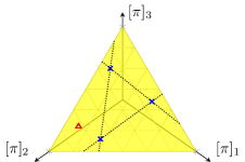
Figure 2: Illustration of the set $\Delta_{y}$ in Theorem 2 (for $X=3$). The blue crosses correspond to $\pi_{1}^{y},\dots,\pi_{X}^{y}$ and the red triangle to $\pi_{X+1}^{y}$. For the conditions of the theorem to be fulfilled, the point $\pi_{X+1}^{y}$ cannot lie on the dashed lines.

II-E Direct Approach to the Inverse Filtering Problem

At a first glance, Problem 1 appears computationally intractable: there are combinatorial elements (due to the unknown sequence of observations) and non-convexity from the products between columns $b_{y}$ of the observation matrix and the transition matrix $P$ in the HMM filter (9).

In order to reconstruct parameters that are consistent with the data (i.e., that satisfy the filter equation (9) and fulfill the non-negativity and sum-to-one constraints imposed by probabilities), a direct approach is to solve the following feasibility problem:

$$\min_{\{y_{k}\}_{k=1}^{N},\,\{b_{y}\}_{y=1}^{Y},\,P} \quad\sum_{k=1}^{N}\left\|\pi_{k}-\frac{\operatorname{diag}(b_{y_{k}})P^{T}\pi_{k-1}}{\mathds{1}^{T}\operatorname{diag}(b_{y_{k}})P^{T}\pi_{k-1}}\right\|$$

s.t. $$\quad y_{k}\in\{1,\dots,Y\},\quad\quad\text{ for }k=1,\dots,N,$$

$$\quad b_{y}\geq 0,\quad\quad\quad\quad\quad\quad\text{ for }y=1,\dots,Y,$$

$$\quad[b_{1}\dots b_{Y}]\mathds{1}=\mathds{1},$$

$$\quad P\mathds{1}=\mathds{1},\quad P\geq 0,$$ (14)

where the choice of norm is arbitrary since the cost is zero for any feasible set of parameters.

The problem (14) is combinatorial (in $\{y_{k}\}_{k=1}^{N}\}$) and non-convex (in $\{b_{y}\}_{y=1}^{Y}$ and $P$) – in other words, it is challenging and computationally costly to obtain a solution. In the next section, we will propose an indirect approach that results in a computationally feasible solution to Problem 1.

III Inverse Filtering by Exploiting
the Structure of the HMM Filter

In this section, we first derive an alternative characterization of the HMM filter (9). The properties of this characterization allow us to formulate an alternative solution to Problem 1. This solution still requires solving a combinatorial problem (a nullspace clustering problem, see Problem 2 below) and is, essentially, equivalent to (14). However, by leveraging insights from its geometrical interpretation, we derive a computationally feasible convex relaxation based on structured sparsity regularization (the fused group LASSO [14]) that permits us to obtain a solution in a computationally feasible manner.

III-A Alternative Characterization of the HMM Filter

Our first result is a variation of the key result derived in [7]. First note that the HMM filter (9) can be rewritten as

$$(\ref{eq:hmm_filter})\iff b_{y_{k}}^{T}P^{T}\pi_{k-1}\pi_{k}=\operatorname{diag}(b_{y_{k}})P^{T}\pi_{k-1},$$ (15)

by simply multiplying by the denominator (which is allowed under Assumption 1). By restructuring (15), we obtain an alternative characterization of the HMM filter (9):

Theorem 3.

Under Assumptions 1 and 2, the HMM filter-update (9) can be equivalently written as

$$(\pi_{k-1}^{T}\otimes[\pi_{k}\mathds{1}^{T}-I])\operatorname{vec}(\operatorname{diag}(b_{y_{k}})P^{T})=0,$$ (16)

for $k=1,\dots,N$.

To see why the reformulation (16) is useful, recall that in Problem 1, we aim to estimate the transition matrix $P$, the observation matrix $B$ and the observations $y_{k}$ given posteriors $\pi_{k}$. Hence, the coefficient matrix $(\pi_{k-1}^{T}\otimes[\pi_{k}\mathds{1}^{T}-I])$ on the left-hand side of (16) is known to us, and all that we aim to estimate is contained in its nullspace.

III-B Reconstructing $P$ and $B$ from Nullspaces

It is apparent from (16) that everything we seek to estimate (i.e., the transition matrix $P$, the observation matrix $B$ and the observations) is accommodated in a vector that lies in the nullspace of a known coefficient matrix. Even so, it is not obvious that the sought quantities can be reconstructed from this. In particular, since a nullspace is only determined up to scalings of its basis vectors, by leveraging (16) we can at most hope to reconstruct the directions of vectors $\operatorname{vec}(\operatorname{diag}(b_{y})P^{T})$:

$$\alpha_{y}\operatorname{vec}(\operatorname{diag}(b_{y})P^{T})\quad\in{\mathbb{R}}^{X^{2}},$$ (17)

for $y=1,\dots,Y$, where $\alpha_{y}\in{\mathbb{R}}_{>0}$ correspond to scale factors.

Can a set of vectors (17) be factorized into $P$ and $B$, and do the undetermined scale factors $\alpha_{y}$ (which, again, are due to the nullspace basis only being determined up to scaling) pose a problem? Our next theorem shows that it can be done. First, however, note that by reshaping (17), we equivalently have access to matrices $a_{y}\operatorname{diag}(b_{y})P^{T}\in{\mathbb{R}}^{X\times X}$ for $y=1,\dots,Y$.

Theorem 4.

Given are matrices $V_{y}\overset{\text{def.}}{=}\alpha_{y}\operatorname{diag}(b_{y})P^{T}$ for $y=1,\dots,Y$, where $P$ and $B=\begin{bmatrix}b_{1}&\dots&b_{Y}\end{bmatrix}$ are HMM parameters satisfying Assumptions 1 and 2, and $\alpha_{y}$ are strictly positive (unknown) scalars. Let $L\overset{\text{def.}}{=}\sum_{y=1}^{Y}V_{y}^{T},$ then the transition matrix $P$ can be reconstructed as

$$P=L\operatorname{diag}(L^{-1}\mathds{1}).$$ (18)

Subsequently, let $\bar{B}\overset{\text{def.}}{=}\begin{bmatrix}V_{1}P^{-T}\mathds{1}&\dots&V_{Y}P^{-T}\mathds{1}\end{bmatrix}$, then the observation matrix can be reconstructed as

$$B=\bar{B}\operatorname{diag}(\bar{B}^{\dagger}\mathds{1}).$$ (19)

The proof of Theorem 19 amounts to algebraically verifying that the relations (18) and (19) hold by employing properties of row-stochastic matrices. The last factor in each equation can be interpreted as a sum-to-one normalization.

III-C How to Compute the Nullspaces?

Theorem 19 gives us a procedure to reconstruct the transition and observation matrices from vectors (17) – i.e., vectors parallel to $\operatorname{vec}(\operatorname{diag}(b_{y})P^{T})$ for $y=1,\dots,Y$. The goal in the remaining part of this section is to compute such vectors from the known coefficient matrices in (16).

If the nullspace of the coefficient matrix of (16) was one-dimensional, we could proceed as in [7]: Since there are only a finite number of values, namely $Y$, that the $y_{k}$:s can take, there are only a finite number of directions in which the nullspaces can point; along the vectors $\operatorname{vec}(\operatorname{diag}(b_{y})P^{T})$ for $y=1,\dots,Y$. Hence, once a coefficient matrix corresponding to each observation $y$ has been obtained, these directions can be reconstructed.

Unfortunately, the nullspace of the coefficient matrix of (16) is not one-dimensional:

Lemma 1.

Under Assumptions 1 and 2, we have that

$$\operatorname{rank}(\pi_{k-1}^{T}\otimes[\pi_{k}\mathds{1}^{T}-I])=X-1.$$ (20)

Since $\operatorname{vec}(\operatorname{diag}(b_{y})P^{T})\in{\mathbb{R}}^{X^{2}}$, the null-space is, in fact, $X^{2}-(X-1)$ dimensional. Below, we demonstrate how, by intersecting multiple nullspaces, we can obtain a one-dimensional subspace (a vector) that is parallel to the vector $\operatorname{vec}(\operatorname{diag}(b_{y})P^{T})$ that we seek.

Remark 2.

The above is not surprising in the light of that every update (9) of the posterior corresponds to $X$ equations. In [7], only the $X$ parameters of $\operatorname{diag}(b_{y})$ had to be reconstructed at each time instant since $P$ was assumed known. Now, instead, we aim to reconstruct the $X^{2}$ parameters of $\operatorname{diag}(b_{y})P^{T}$, which cannot be done with just one update (i.e., with $X$ equations). Hence, we will need to employ the equations from several updates.

III-D Special Case: Known Sequence of Observations

To make the workings of our proposed method more transparent, suppose for the moment that we have access to the sequence of observations $y_{1},\dots,y_{N}$ that were processed by the filter (9). By Theorem 3, we know that the vector $\operatorname{vec}(\operatorname{diag}(b_{y_{k}})P^{T})$ lies in the nullspace of the coefficient matrix $(\pi_{k-1}^{T}\otimes[\pi_{k}\mathds{1}^{T}-I])$ for all $k=1,\dots,N$. If we consider only the time instants when a certain observation, say $y$, was processed, then the vector $\operatorname{vec}(\operatorname{diag}(b_{y})P^{T})$ lies in the nullspace of all the corresponding coefficient matrices:

$$\operatorname{vec}(\operatorname{diag}(b_{y})P^{T})\in\bigcap\limits_{k:\,y_{k}=y}\ker{(\pi_{k-1}^{T}\otimes[\pi_{k}\mathds{1}^{T}-I])},$$ (21)

for $y=1,\dots,Y$. Now, if the intersection on the right-hand side of (21) is one-dimensional, this gives us a way to reconstruct the direction of $\operatorname{vec}(\operatorname{diag}(b_{y})P^{T})$ – in this case,

$$\operatorname{span}(\operatorname{vec}(\operatorname{diag}(b_{y})P^{T}))=\bigcap\limits_{k:\,y_{k}=y}\ker{(\pi_{k-1}^{T}\otimes[\pi_{k}\mathds{1}^{T}-I])},$$ (22)

and we simply compute the one-dimensional intersection. Recall that the next step would then be to factorize these directions into the products $P$ and $B$ via Theorem 19.

The identifiability result of Theorem 2 tells us that this happens when there exists a subsequence $\Delta_{y}\subset\{\pi_{k}\}_{k:y_{k}=y}$, that satisfies the criteria in Theorem 2.

Remark 3.

In practice, roughly $X$ updates, for each $y$, should be enough (see Remark 2). A pessimistic estimate of how many samples will be required for this can be obtain via similar reasoning as in [7, Lemma 3]: if $B\geq\beta>0$ elementwise, then on the order of $\beta^{-1}YX^{2}$ samples are expected to suffice.

III-E Inverse Filtering via Nullspace Clustering

Problem 1 is complicated by the fact that in the inverse filtering problem, we do not have access to the sequence of observations – we only observe a sequence of posteriors. Thus, we do not know at what time instants a certain observation $y$ was processed and, hence, which nullspaces to intersect, as in (22), to obtain a vector parallel to $\operatorname{vec}(\operatorname{diag}(b_{y})P^{T})$.

An abstract version of the problem can be posed as follows:

Problem 2 (Nullspace Clustering).

Given is a set of matrices $\{A_{k}\}_{k=1}^{N}$ that can be divided into $Y$ subsets (clustered) such that the intersection of the nullspaces of the matrices in each subset is one-dimensional. That is, there are numbers $\{y_{k}\}_{k=1}^{N}$ with $y_{k}\in\{1,\dots,Y\}$ such that,

$$\bigcap\limits_{k:\,y_{k}=y}\ker{A_{k}}=\operatorname{span}(v_{y}),$$ (23)

for some vector $v_{y}$ with $y=1,\dots,Y$. Find the vectors $\{v_{y}\}_{y=1}^{Y}$ that span the intersections.

We provide a graphical illustration of the nullspace clustering problem in Fig. 3. Note that, in our instantiation of the problem, $A_{k}=(\pi_{k-1}^{T}\otimes[\pi_{k}\mathds{1}^{T}-I])$ is the coefficient matrix of the HMM filter (16), and each vector $v_{y}=\operatorname{vec}(\operatorname{diag}(b_{y})P^{T})$ is what we aim to reconstruct.

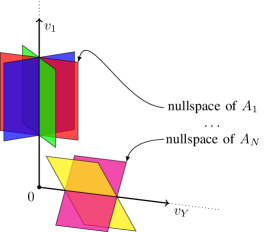
Figure 3: We are given a set of subspaces parametrized by the nullspaces of matrices $A_{1},\dots,A_{N}$. These subspaces have the property that each subspace contains one of the $Y$ vectors $v_{1},\dots,v_{Y}$. In the nullspace clustering problem (Problem 2), the aim is to find the (directions of) vectors $v_{1},\dots,v_{Y}$.

The problem was simplified in the previous section, since by knowing the observations $y_{1},\dots,y_{N}$, we know which vector each subspace is generated about (i.e., the subset assignments) and can simply intersect the subspaces in each subset to obtain the vectors $v_{1},\dots,v_{Y}$. By not having direct access to the sequence of observations, the problem becomes combinatorial; which nullspaces should be intersected? Albeit a solution can be obtained via mixed-integer optimization in much the same fashion as in (14) – since Problem 2 is merely a reformulation of the original problem – such an approach can be highly computationally demanding.

We propose instead the following two-step procedure that consists of, first, a convex relaxation, and second, a refinement step using local heuristics. We emphasize that if the two steps succeed, then there is nothing approximate about the solution we obtain – the directions of the vectors $v_{y}$ are obtained exactly.

Step 1. Convex Relaxation

Compute a solution to the convex problem

$$\min_{\{w_{k}\}_{k=1}^{N}} \quad\sum_{i=1}^{N}\sum_{j=1}^{N}\|w_{i}-w_{j}\|_{\infty}$$

s.t. $$\quad A_{k}w_{k}=0,\quad\text{ for }k=1,\dots,N,$$

$$\quad w_{k}\geq 1,\hskip 22.76228pt\text{ for }k=1,\dots,N,$$ (24)

which aims to find $N$ vectors that each lie in the nullspace of the corresponding matrix $A_{k}$, and that, by the objective function, are promoted to coincide via a fused group LASSO [14]. That is, the set $\{w_{k}\}_{k=1}^{N}$ is sparse in the number of unique vectors. This is a relaxation because we have dropped the hard constraint of there only being exactly $Y$ different vectors. The constraint $w_{k}\geq 1$ assures that we avoid the trivial case $w_{k}=0$ for all $k$. The $\|\cdot\|_{\infty}$-norm is used for convenience since problem (24) can then be reformulated as a linear program.

Step 2. Refinement via Spherical Clustering

The solution of (24) does not completely solve our problem for two reasons: i) it is not guaranteed to return precisely $Y$ unique basis vectors, and ii) it does not tell us to which subset the nullspace of each $A_{k}$ should be assigned (i.e., we still do not know which nullspaces to intersect).

In order to address these two points, we perform a local refinement using spherical k-means clustering [28] on the set of vectors $\{w_{k}\}_{k=1}^{N}$ resulting from (24). This provides us with a set of $Y$ centroid vectors, as well as a cluster assignment of each vector $w_{k}$. We employ the spherical version of k-means since we seek nullspace basis vectors – the appropriate distance measure is angular spread, and not the Euclidean norm employed in standard k-means clustering.

Now, the centroid vectors should provide good approximations of the vectors we seek (since $\{w_{k}\}_{k=1}^{N}$ are expected to be spread around the intersections of the nullspaces by the sparsity promoting objective in (24)). However, they do not necessarily lie in any nullspace since their computation is unconstrained. To obtain an exact solution to the problem, we go through the $w_{k}$:s assigned to each cluster in order of distance to the cluster’s centroid and intersect the corresponding $A_{k}$:s’ nullspaces until we obtain a one-dimensional intersection.

It should be underlined that when an intersection that is one-dimensional has been obtained, the (direction of) the vector $v_{y}$ has been computed exactly. Recall that in our instantiation of the problem, each vector $v_{y}=\operatorname{vec}(\operatorname{diag}(b_{y})P^{T})$, so that once these have been reconstructed, they can be decomposed into the transition matrix $P$ and the observation matrix $B$ according to Theorem 19.

Figure 4: Schematic illustration of the setup in (25)-(28). An autonomous adversary measures our state $x_{k}$ as $y_{k}$ via a sensor $B$. A mismatched (note that estimates $\hat{P}$ and $\hat{B}$ are employed) Bayesian filter is used to compute its posterior $\pi_{k}$ of our state. Based on this posterior and a policy $G$, a public action $u_{k}$ is taken. In the remote sensor calibration problem (Problem 3), the aim is to estimate the adversary’s sensor $B$ (which is, in general, different from $\hat{B}$).

Remark 4.

Theorem 19 assumes that we are given the matrices $V_{y}$ sorted according to the actual labeling of the HMM’s observations. If we use the method described above, the vectors are only obtained up to permutations of the observation labels (this corresponds to the label assigned to each cluster in the spherical k-means algorithm). Hence, in practice, we will obtain $B$ up to permutations of its columns.

III-F Summary of Proposed Algorithm

For convenience, the complete procedure for solving Problem 1 is summarized in Algorithm 1. It should be pointed out that the algorithm will fail to determine a solution to Problem 1 if it can not intersect down to a one-dimensional subspace for some $y$. Then, the direction of the vector $\operatorname{vec}(\operatorname{diag}(b_{y})P^{T})$ cannot be determined uniquely, and the full set of these vectors is required in Theorem 19. This is because this observation has not been measured enough times, or that the convex relaxation has failed. As noted in Remark 2, we expect on the order of $YX^{2}$ posteriors to be needed for the procedure to succeed – we explore this further in the numerical examples in Section V.

Remark 5.

Once $P$ and $B$ have been reconstructed via Algorithm 1, to obtain the sequence of observations, simply check which observation $y\in\mathcal{Y}$ that maps $\pi_{k-1}$ to $\pi_{k}$ via the HMM filter (9) for $k=1,\dots,N$. This can be done in linear time (in $N$).

Algorithm 1 Inverse Filtering (Solution to Problem 1)

0:  Sequence of posteriors $\{\pi_{k}\}_{k=1}^{N}$, dimension $Y$

1:  Compute the coefficient matrices $A_{k}=(\pi_{k-1}^{T}\otimes[\pi_{k}\mathds{1}^{T}-I])$ of (16) for $k=1,\dots,N$.

2:  Compute a solution $\{w_{k}\}_{k=1}^{N}$ to the convex problem (24).

3:  Run spherical k-means clustering for $Y$ clusters on the vectors $\{w_{k}\}_{k=1}^{N}$

4:  for each of the $Y$ clusters do

5:     $k$-set = $\{\}$

6:     for each $w_{k}$ in order of increasing distance to its cluster’s centroid do

7:        Compute intersection of current, and past, corresponding $A_{k}$:s’ nullspaces:     i) Add $k$ to $k$-set,    ii) Compute $\bigcap_{k\in k\text{-set}}\ker{A_{k}}$

8:        if intersection is one-dimensional then

9:           Save as $v_{y}$ and proceed to the next cluster.

10:        end if

11:     end for

12:  end for

13:  Factorize $\{v_{y}\}_{y=1}^{Y}$ into $P$ and $B$ using equations (18) and (19), respectively.

14:  To obtain the corresponding sequence of observations, see Remark 5.

IV Applications of Inverse Filtering to Counter-Adversarial Autonomous Systems

During the last decade, the importance of defense against cyber-adversarial and autonomous treats has been highlighted on numerous occasions – e.g., [4, 29, 30]. In this section, we illustrate how the results in the previous section can be generalized when i) the posteriors from the Bayesian filter are observed in noise, and ii) the filtering system is mismatched. The problem is motived by remotely calibrating (i.e., estimating) the sensors of an autonomous adversary by observing its actions.

IV-A Counter-Adversarial Autonomous Systems

Consider an adversary that employs an autonomous filtering and control system that estimates our state and takes actions based on a control policy. The goal in the design of a counter-adversarial autonomous (CAA) system is to infer information private to the adversary, and to predict and guard against its future actions [4, 5, 6].

Formally, it can be interpreted as a two-player game in the form of a partially observed Markov decision process (POMDP; [1]), where information is partitioned between two players: us and the adversary. The model (1)-(2) is now generalized to:

$$\text{us:}\quad\!x_{k} \sim P_{x_{k-1},x}=p(x|x_{k-1}),\,x_{0}\sim\pi_{0}$$ (25)

$$\text{adversary:}\quad\!y_{k} \sim B_{x_{k},y}=p(y|x_{k}),$$ (26)

$$\text{adversary:}\quad\!\pi_{k} =T(\pi_{k-1},y_{k};\hat{P},\hat{B}),$$ (27)

$$\text{adversary \& us:}\quad\!u_{k} \sim G_{\pi_{k},u}=p(u|\pi_{k}),$$ (28)

which should be interpreted as follows. The state $x_{k}\in\mathcal{X}$, with initial condition $\pi_{0}$, is our state that we use to probe the adversary. The observation $y_{k}\in\mathcal{Y}$ is made by the adversary, who subsequently computes its posterior (in this setting, we refer to it also as a belief) $\pi_{k}$ of our state using the Bayesian filter $T$ from (5). Note that the adversary does not have perfect knowledge of our transition kernel $P$ nor its sensor $B$; it uses estimates $\hat{P}$ and $\hat{B}$ in (27). Finally, the adversary takes an action $u_{k}\in\mathcal{U}$, where $\mathcal{U}$ is an action set, according to a control policy $G$ based on its belief.

A schematic overview is drawn in Fig. 4, where the dashed boxes demarcate information between the players (public means both us and the adversary have access).

IV-B Remote Calibration of an Adversary’s Sensors

Various questions can be asked that are of importance in the design of a CAA system. The specific problem we consider is that of remotely calibrating the adversary’s sensor:

Problem 3 (Remote Calibration of Sensors in CAA Systems).

Consider the CAA system (25)-(28). Given knowledge of our realized state sequence $x_{0},x_{1},x_{2},\dots$, our transition kernel $P$ and the actions taken by the adversary $u_{1},u_{2},\dots$; estimate the observation likelihoods $B$ of the adversary’s sensor.

A few remarks on the above problem: Our final targets are the likelihoods $B$, not the adversary’s own estimate $\hat{B}$. Previous work [7, 5, 6] that considered the above problem, or variations thereof, assumed that the adversary’s filter was perfectly matched (i.e., $\hat{P}=P$ and $\hat{B}=B$) and, hence, that $P$ was known to the adversary. We generalize to the more challenging setup of a mismatched filtering system, and will, hence, have to estimate the adversary’s estimate of our transition kernel. Albeit outside the scope of this paper, with a solution to Problem 3 in place, a natural extension is the input design problem adapted to CAA systems: How to design our transition kernel $P$ so as to i) maximally confuse the adversary, or ii) optimally estimate its sensor?

In order to connect with the results of the previous section, we consider only discrete CAA systems – that is, where the state space $\mathcal{X}=\{1,\dots,X\}$ and observation space $\mathcal{Y}=\{1,\dots,Y\}$ are discrete. Moreover, we assume that the dimensions $X$ and $Y$ are known to both us and the adversary.

IV-C Reconstructing Beliefs from Actions

The feasibility of Problem 3 clearly depends on the adversary’s policy – for example, if the policy is independent of its belief $\pi_{k}$, we can hardly hope to estimate anything regarding its sensors. A natural assumption is that the adversary is rational and that its policy $G$ is based on optimizing its expected cost[31, 32, 33]:

$$\min_{u_{k}}\quad \mathbb{E}_{x_{k}}\left\{c(x_{k},u_{k})\,|\,y_{1},\dots,y_{k}\right\}$$

s.t. $$u_{k}\in\mathcal{C},$$ (29)

where $c(x,u)$ is a cost function that depends on our state and an action $u\in\mathcal{C}\subset\mathcal{U}$, with $\mathcal{C}$ a constraint set. That is, the adversary selects an action by minimizing the cost it is expected to receive in the next time instant.

Recall that the results in Section III reconstruct filter parameters from posteriors. In order to leverage these results for Problem 3, we first need to obtain the adversary’s posterior distributions from its actions. This is discussed to a longer extent in [5, 6], in a Bayesian framework, and in [34] in an analytic setting. We will use, and briefly recap, the main results of [34] below.

However, first of all, even with a structural form such as (29) in place, the set of potential policies is still infinite. Without any prior assumptions on the adversary’s preferences and constraints, it is impossible to conclusively infer specifics regarding its posteriors. In [34], it is assumed that:

Assumption 3.

We know the adversary’s cost function $c(x,u)$ and its constraint set $\mathcal{C}$. Moreover, $c(x,u)$ is convex and differentiable in $u$.

Under this assumption, the full set of posteriors that the adversary could have had at any time instant was characterized in [34] using techniques from inverse optimization [35]. Some regularity conditions are needed to guarantee that a unique posterior can be reconstructed – in general, several posteriors could result in the same action, which would complicate our upcoming treatment of Problem 3. One set of such conditions is the following:

Assumption 4.

The adversary’s decision is unconstrained in Euclidean space, i.e., $\mathcal{C}=\mathcal{U}={\mathbb{R}}^{U}$ for some dimension $U$. The matrix

$$F(u)=\begin{bmatrix}\nabla_{u}c(1,u)&\dots&\nabla_{u}c(X,u)\\ 1&\dots&1\end{bmatrix}$$ (30)

has full column rank when evaluated at the observed actions $u_{1},\dots,u_{N}$.

This assumption says, roughly, that the cost functions defined in (29) are “different enough”, and that no information is truncated via active constraints. The key result is then the following:

Theorem 5.

Under Assumptions 3 and 30, the posteriors of an adversary selecting actions according to (29) can be uniquely reconstructed by us from its actions as

$$\pi_{k}=F(u_{k})^{\dagger}\begin{bmatrix}0&\dots&0&1\end{bmatrix}^{T},$$ (31)

for $k=1,\dots,N$, where the matrix $F(u)$ is defined in (30) and the last vector consists of $X$ zeros and a single one.

The theorem follows directly from [34, Theorem 1] and the linear independence of columns of the matrix $F(u)$ in (30) – details are available in the appendix.

IV-D Solution to the Remote Sensor Calibration Problem

We will now outline a solution to Problem 3 that leverages the inverse filtering algorithms from Section III.

Step 1. Reconstruct Posteriors

Using Theorem 5, reconstruct the adversary’s sequence of posteriors $\pi_{1},\dots,\pi_{N}$ from its observed actions and the structural form of its policy.

Step 2. Reconstruct $\hat{P}$ and $\hat{B}$

Apply Algorithm 1 from Section III on the sequence of posteriors. Note that the posteriors were computed by the adversary using a mismatched filter (27) – i.e., as $T(\pi,y;\hat{P},\hat{B})$ –, so that Algorithm 1 reconstructs the adversary’s estimates $\hat{P}$ and $\hat{B}$ of our transition matrix $P$ and its sensor $B$.

Step 3. Reconstruct the Observations

As mentioned in Remark 5, once the filter’s parameters are known it is trivial to reconstruct the corresponding sequence of observations $y_{1},\dots,y_{N}$.

Step 4. Calibrate the Adversary’s Sensor

We now have access to the observations $y_{1},\dots,y_{N}$ that were realized by the HMM $(P,B)$ and, by the setup of the CAA system (25)-(28), the corresponding state sequence $x_{1},\dots,x_{N}$. With this information, we can compute our maximum likelihood estimate $\check{B}$ of the adversary’s sensor $B$ via

$$[\check{B}]_{ij}=\frac{\sum_{k=1}^{N}\text{I}\{x_{k}=i,y_{k}=j\}}{\sum_{k=1}^{N}\text{I}\{x_{k}=i\}},$$ (32)

which corresponds to the M-step in the expectation-maximization (EM) algorithm for HMMs – see, e.g., [36, Section 6.2.3]. This completes the solution to Problem 3.

Discussion

It is worth making a few remarks at this point. First of all, it should be underlined that $\hat{B}\neq\check{B}$ – that is, our estimate $\check{B}$ is not necessarily equal to that of the adversary $\hat{B}$. In fact, our estimate depends on the number $N$ of observed actions and is, as such, improving over time by the asymptotic consistency of the maximum likelihood estimate. If the adversary does not recalibrate its estimate $\hat{B}$ online, then for large enough $N$, our estimate will eventually be more accurate than the adversary’s own estimate.

Moreover, the steps in Section IV-D are independent of the accuracy of the adversary’s estimates $\hat{P}$ and $\hat{B}$ (as long as they fulfill Assumptions 1 and 2) since we are exploiting the algebraic structure of its filter. This means that, even if the adversary employs a bad estimate of our transition matrix $P$, as long as it is taking actions, we can improve our estimate of its sensor $B$.

Finally, if the setup is modified so that we do not have access to the transition matrix $P$ or the realized state sequence in (25), then the step (32) would be replaced by the full EM algorithm. This would compute our estimates $\check{P}$ and $\check{B}$ of the system’s transition matrix $P$ and the adversary’s sensor $B$ based on the reconstructed observations made by the adversary. Again, by the asymptotic properties of the maximum likelihood estimate, the accuracy of these estimates (that depend on $N$) will eventually surpass those of the adversary.

V Numerical Examples

In this section, we evaluate and illustrate the proposed inverse filtering algorithms in numerical examples. All simulations were run in MATLAB R2018a on a 1.9 GHz CPU.

V-A Reconstructing $P$ and $B$ via Inverse Filtering

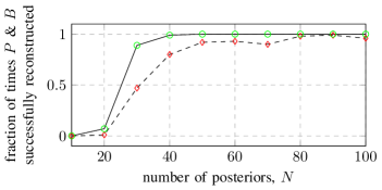
Figure 5: In Problem 1, we obtain a sequence $\{\pi_{k}\}_{k=1}^{N}$ of posteriors from an HMM filter (9). Out of 100 realizations, for each value of $N$, we compute the fraction of times that Algorithm 1 successfully reconstructs the transition matrix $P$ and the observation matrix $B$ of the HMM (red diamonds). We also plot the success rate of an oracle method (green circles) that has access to the observations. With around $N=50$ posteriors, the algorithm succeeds frequently.

Recall that Problem 1 aims to reconstruct HMM parameters given a sequence of posterior distributions. Algorithm 1 is deterministic, but there is randomness in terms of the data (the realization of the HMM) which can cause the algorithm to fail to reconstruct the HMM’s parameters. This can happen for three different reasons: First, if a certain observation has been measured too few times then there is fundamentally too few equations available to reconstruct the parameters – see Remark 2 (in Section III-C). Second, if too few independent equations have been generated, we do not have identifiability and cannot intersect to a one-dimensional subspace in (22) – see Theorem 2. Third, we rely on a convex relaxation to solve the original combinatorial problem. This is a heuristic and it is not guaranteed to converge to a solution of the original problem. Hence, in these simulations, we estimate the probability of the algorithm succeeding (with respect to the realization of the HMM data).

In order to demonstrate that the assumptions we have made in the paper are not strict, we consider the following HMM:

$$P=\begin{bmatrix}0&\nicefrac{{1}}{{2}}&0&0&\nicefrac{{1}}{{2}}\\ \nicefrac{{1}}{{2}}&0&\nicefrac{{1}}{{2}}&0&0\\ 0&\nicefrac{{1}}{{2}}&0&\nicefrac{{1}}{{2}}&0\\ 0&0&\nicefrac{{1}}{{2}}&0&\nicefrac{{1}}{{2}}\\ \nicefrac{{1}}{{2}}&0&0&\nicefrac{{1}}{{2}}&0\\ \end{bmatrix},\;B=\begin{bmatrix}\nicefrac{{2}}{{5}}&\nicefrac{{2}}{{5}}&\nicefrac{{1}}{{5}}\\ \nicefrac{{2}}{{5}}&\nicefrac{{2}}{{5}}&\nicefrac{{1}}{{5}}\\ \nicefrac{{2}}{{5}}&\nicefrac{{1}}{{5}}&\nicefrac{{2}}{{5}}\\ \nicefrac{{1}}{{5}}&\nicefrac{{2}}{{5}}&\nicefrac{{2}}{{5}}\\ \nicefrac{{1}}{{5}}&\nicefrac{{2}}{{5}}&\nicefrac{{2}}{{5}}\\ \end{bmatrix}.$$ (33)

Note that its transition matrix corresponds to a random walk, which violates Assumption 1. We consider a reconstruction successful if the error in norm is smaller than $10^{-3}$ for both $P$ and $B$. We generated 100 independent realizations for a range of values of $N$ (the number of posteriors). The fractions of times the algorithms were successful are plotted in Fig. 5 with red diamonds for Algorithm 1, and with green circles for an oracle method that has access to the corresponding sequence of observations. The oracle method provides an upper bound on the success rate (if it fails, it is not possible to uniquely reconstruct the HMM parameters, as discussed above). The gap between the curves is due to the convex relaxation.

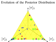
Figure 6: A realization of the set $\{\pi_{k}\}_{k=1}^{50}$, corresponding to HMM (34), illustrated on the simplex. The points are labeled according to what observation was measured: $y=1$ (red triangle), $y=2$ (blue cross), $y=3$ (green circle). To fulfill the conditions of Theorem 2, the points corresponding to each observation cannot all lie on the lines connecting any two points – see Fig. 2.

A few things should be noted from Fig. 5. First, with only around 50 posteriors from the HMM filter, the fraction of times the algorithm succeeds in solving Problem 1 is high. It was noted in Remark 3 (in Section III-D), that since $B\geq\nicefrac{{1}}{{5}}\overset{\text{def.}}{=}\beta$, a rough estimate is that $\beta^{-1}YX^{2}=375$ posteriors should suffice – however, as is clear from Fig. 5, this is a very conservative estimate since the algorithm is very successful already with around 50 posteriors. Second, the gap between the two curves is small – hence, the convex relaxation is successful in achieving a solution to the original combinatorial problem. Finally, it should be mentioned that with 50 posteriors, the run-time is approximately thirty seconds.

V-B Evolution of the Posterior Distribution

Next, to illustrate the conditions of Theorem 2, we plot the set $\{\pi_{k}\}_{k=1}^{50}$ on the simplex. To be able to visualize the data, we now consider an HMM with dimension $X=3$:

$$P=\begin{bmatrix}0.8&0.1&0.1\\ 0.05&0.9&0.05\\ 0.2&0.1&0.7\end{bmatrix},\quad B=\begin{bmatrix}0.7&0.1&0.2\\ 0.1&0.8&0.1\\ 0.05&0.05&0.9\end{bmatrix}.$$ (34)

In Fig. 6, each posterior has been marked according to which observation was subsequently measured. We can clearly find four posteriors, for each observation, that are sufficiently disperse (see the illustration in Fig. 2), and hence fulfill the conditions for Theorem 2 that guarantees a unique solution.

The results of simulations with the same setup as before are shown in Fig. 7, and similar conclusions can be drawn. First, with around 50 posteriors, the algorithm has a high success rate. Second, the bound in Remark 3 (in Section III-D) postulate an expected number of posteriors of 540, which again is conservative.

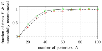
Figure 7: Same setup as in Fig. 5, but for the HMM (34). With access to around 50 posteriors, Algorithm 1 succeeds in reconstructing $P$ and $B$ very frequently.

VI Conclusions and Future work

In this paper, we considered inverse filtering problems for hidden Markov models (HMMs) with finite observation spaces. We proposed algorithms to reconstruct the transition kernel, the observation likelihoods and the measured observations from a sequence of posterior distributions computed by an HMM filter. Our key algorithm is a two-step procedure based on a convex relaxation and a subsequent local refinement. We discussed and derived conditions for identifiability in inverse filtering. As an application of our results, we demonstrated how the proposed algorithms can be employed in the design of counter-adversarial autonomous systems: How to remotely calibrate the sensors of an autonomous adversary based on its actions? Finally, the algorithms were evaluated and verified in numerical simulations.

In the future, we would like to analyze the nullspace clustering problem further and see if it applies to other settings. We would also like to generalize the setup to other policy-structures of the adversary – for example, when its action set is discrete.

Appendix A Proof of Theorem 1

To prove Theorem 1, we will use the following auxiliary lemma:

Lemma 2.

Let $A\in{\mathbb{R}}^{X\times X}$ and $M\in{\mathbb{R}}^{X\times X}$ be two non-singular matrices. If

$$Ax=\kappa(x)Mx,\qquad\forall x\in\Delta,$$ (35)

where $\kappa(x)$ is a non-zero scalar, and $\Delta=\{x\in{\mathbb{R}}^{X}:x\geq 0,\mathds{1}^{T}x=1\}$ is the unit simplex, then

$$A=\kappa M,$$ (36)

where $\kappa$ is a non-zero constant scalar.

Proof.

Consider the $i$th Cartesian basis vector $e_{i}\in\Delta$:

$$Ae_{i}=\kappa(e_{i})Me_{i}.$$ (37)

Concatenate (37) for $i=1,\dots,X$, to get

$$A\begin{bmatrix}e_{1}&\dots&e_{X}\end{bmatrix} =M\begin{bmatrix}\kappa(e_{1})e_{1}&\dots&\kappa(e_{X})e_{X}\end{bmatrix}\implies$$

$$A =M\begin{bmatrix}\kappa(e_{1})&&0\\ &\ddots&\\ 0&&\kappa(e_{X})\end{bmatrix}.$$ (38)

Next, consider any vector on the simplex with non-zero components:

$$x=[x]_{1}e_{1}+\dots+[x]_{X}e_{X}\qquad\in\Delta,$$ (39)

such that $[x]_{i}\neq 0$ for $i=1,\dots,X$. Introducing (38) in (35) for this $x$ yields

$$M \begin{bmatrix}\kappa(e_{1})&&0\\ &\ddots&\\ 0&&\kappa(e_{X})\end{bmatrix}\left([x]_{1}e_{1}+\dots+[x]_{X}e_{X}\right)$$

$$=\kappa(x)M\left([x]_{1}e_{1}+\dots+[x]_{X}e_{X}\right)\implies$$

$$\kappa(e_{1}) [x]_{1}e_{1}+\dots+\kappa(e_{X})[x]_{X}e_{X}$$

$$\hskip 31.2982pt=\kappa(x)[x]_{1}e_{1}+\dots+\kappa(x)[x]_{1}e_{X},$$ (40)

where in the implication we have multiplied by $M^{-1}$ from the left and simplified the expression. Since the $e_{i}$:s are linearly independent, consider any component of (40):

$$\kappa(e_{i})[x]_{i} =\kappa(x)[x]_{i}\implies$$

$$\kappa(e_{i}) =\kappa(x),$$ (41)

for $i=1,\dots,X$, since $[x]_{i}\neq 0$. In other words,

$$\kappa(e_{1})=\dots=\kappa(e_{X})=\kappa(x)\overset{\text{def.}}{=}\kappa$$ (42)

is constant. Introducing this in (38) yields

$$A =M\begin{bmatrix}\kappa&&0\\ &\ddots&\\ 0&&\kappa\end{bmatrix}$$

$$=\kappa M.$$ (43)

∎

To employ Lemma 2, we reformulate (13) as follows:

$$T(\pi,y;P,B) =T(\pi,y;\tilde{P},\tilde{B})\implies$$

$$\frac{\operatorname{diag}(b_{y})P^{T}\pi}{\mathds{1}^{T}\operatorname{diag}(b_{y})P^{T}\pi} =\frac{\operatorname{diag}(\tilde{b}_{y})\tilde{P}^{T}\pi}{\mathds{1}^{T}\operatorname{diag}(\tilde{b}_{y})\tilde{P}^{T}\pi}\implies$$

$$\operatorname{diag}(b_{y})P^{T}\pi =\frac{\mathds{1}^{T}\operatorname{diag}(b_{y})P^{T}\pi}{\mathds{1}^{T}\operatorname{diag}(\tilde{b}_{y})\tilde{P}^{T}\pi}\operatorname{diag}(\tilde{b}_{y})\tilde{P}^{T}\pi,$$ (44)

which holds for all $\pi\in\Delta$ and $y=1,\dots,Y$.

Next, we consider (44) for a fixed $y$, and note that the matrices $\operatorname{diag}(b_{y})P^{T}$ and $\operatorname{diag}(\tilde{b}_{y})\tilde{P}^{T}$ are non-singular (by Assumptions 1 and 2). Lemma 2 then yields that

$$\operatorname{diag}(b_{y})P^{T} =\alpha(y)\operatorname{diag}(\tilde{b}_{y})\tilde{P}^{T}\implies$$

$$P\operatorname{diag}(b_{y}) =\tilde{P}\alpha(y)\operatorname{diag}(\tilde{b}_{y}),$$ (45)

where $\alpha(y)\in{\mathbb{R}}$ is a scalar and which holds for $y=1,\dots,Y$.

If we sum equations (45) over $y$, and use the fact that $B$ is a stochastic matrix,

$$\sum_{y=1}^{Y}P\operatorname{diag}(b_{y}) =\sum_{y=1}^{Y}\tilde{P}\alpha(y)\operatorname{diag}(\tilde{b}_{y}), \implies$$

$$P =\tilde{P}\sum_{y=1}^{Y}\alpha(y)\operatorname{diag}(\tilde{b}_{y}),$$ (46)

and then right-multiply by $\mathds{1}$, and use that $P$ is a stochastic matrix, we obtain

$$P\mathds{1} =\tilde{P}\sum_{y=1}^{Y}\alpha(y)\operatorname{diag}(\tilde{b}_{y})\mathds{1}, \implies$$

$$\mathds{1} =\tilde{P}\sum_{y=1}^{Y}\alpha(y)\tilde{b}_{y}.$$ (47)

Pre-multiplying by $\tilde{P}^{-1}$ yields

$$\tilde{P}^{-1}\mathds{1} =\tilde{P}^{-1}\tilde{P}\sum_{y=1}^{Y}\alpha(y)\tilde{b}_{y} \implies$$

$$\mathds{1} =\sum_{y=1}^{Y}\alpha(y)\tilde{b}_{y},$$ (48)

where we have used the fact that the row-sums of the inverse of a (row) stochastic matrix are all equal to one. By applying the $\operatorname{diag}()$-operation to (48), we see that

$$I=\sum_{y=1}^{Y}\alpha(y)\operatorname{diag}(\tilde{b}_{y}),$$ (49)

which when introduced in (46) yields that

$$\tilde{P}=P.$$ (50)

Next, note that (48) can be rewritten as $\mathds{1}=\tilde{B}\begin{bmatrix}\alpha(1)&\dots&\alpha(Y)\end{bmatrix}^{T}$. We know that $\tilde{B}\mathds{1}=\mathds{1}$, since it is a stochastic matrix, and that $\tilde{B}$ has full column rank by assumption. Hence, $\mathds{1}=\begin{bmatrix}\alpha(1)&\dots&\alpha(Y)\end{bmatrix}^{T}$. This yields

$$b_{y}=\tilde{b}_{y},$$ (51)

for $y=1,\dots,Y$, from (45) by first pre-multiplying by $P^{-1}$.

The other direction is trivial: if $P=\tilde{P}$ and $B=\tilde{B}$, then $T(\pi,y;P,B)=T(\pi,y;\tilde{P},\tilde{B})$ for all $\pi\in\Delta$ and each $y=1,\dots,Y$ by (9):

$$\frac{\operatorname{diag}(b_{y})P^{T}\pi}{\mathds{1}^{T}\operatorname{diag}(b_{y})P^{T}\pi}=\frac{\operatorname{diag}(\tilde{b}_{y})\tilde{P}^{T}\pi}{\mathds{1}^{T}\operatorname{diag}(\tilde{b}_{y})\tilde{P}^{T}\pi}.$$ (52)

Appendix B Proof of Theorem 2

We begin by giving a generalization of Lemma 2:

Lemma 3.

Let $A\in{\mathbb{R}}^{X\times X}$ and $M\in{\mathbb{R}}^{X\times X}$ be two non-singular matrices and $\mathcal{Z}=\{z_{1},\dots,z_{X},z_{X+1}\}$ be a set of vectors where $z_{1},\dots,z_{X}\in{\mathbb{R}}^{X}$ are linearly independent and the last vector when expressed in this basis has non-zero components – that is, $z_{X+1}\in{\mathbb{R}}^{X}$ can be written

$$z_{X+1}=[\beta]_{1}z_{1}+\dots+[\beta]_{X}z_{X},$$ (53)

with $\beta\in{\mathbb{R}}^{X}$ and $[\beta]_{i}\neq 0$ for $i=1,\dots,X$. If

$$Ax=\kappa(x)Mx,\qquad\forall x\in\mathcal{Z},$$ (54)

where $\kappa(x)$ is a non-zero scalar, then

$$A=\kappa M,$$ (55)

where $\kappa$ is a non-zero constant scalar.

Proof.

For the $i$th vector in $\mathcal{Z}$, we have by (54) that

$$Az_{i}=\kappa(z_{i})Mz_{i},$$ (56)

which can be concatenated to

$$A\begin{bmatrix}z_{1}&\dots&z_{X}\end{bmatrix} =M\begin{bmatrix}\kappa(z_{1})z_{1}&\dots&\kappa(z_{X})z_{X}\end{bmatrix}\implies$$

$$AZ =M\begin{bmatrix}z_{1}&\dots&z_{X}\end{bmatrix}\begin{bmatrix}\kappa(z_{1})&&0\\ &\ddots&\\ 0&&\kappa(z_{X})\end{bmatrix}$$

$$=MZ\begin{bmatrix}\kappa(z_{1})&&0\\ &\ddots&\\ 0&&\kappa(z_{X})\end{bmatrix},$$ (57)

where we have denoted $Z=\begin{bmatrix}z_{1}&\dots&z_{X}\end{bmatrix}$.

We can rewrite (53) with this definition of $Z$ as

$$z_{X+1}=Z\beta,$$ (58)

which together with (57) yields

$$Az_{X+1} =AZ\beta$$

$$=MZ\begin{bmatrix}\kappa(z_{1})&&0\\ &\ddots&\\ 0&&\kappa(z_{X})\end{bmatrix}\beta.$$ (59)

Next, by employing (54) for $z_{X+1}$ and using (58), we obtain

$$Az_{X+1} =\kappa(z_{X+1})Mz_{X+1}$$

$$=\kappa(z_{X+1})MZ\beta.$$ (60)

Equating (59) and (60) yields

$$MZ\begin{bmatrix}\kappa(z_{1})&&0\\ &\ddots&\\ 0&&\kappa(z_{X})\end{bmatrix}\beta =\kappa(z_{X+1})MZ\beta\implies$$

$$\begin{bmatrix}\kappa(z_{1})&&0\\ &\ddots&\\ 0&&\kappa(z_{X})\end{bmatrix}\beta =\kappa(z_{X+1})\beta,$$ (61)

by multiplying by the inverse of $MZ$ from the left. The $i$th component of (61) is

$$\kappa(z_{i})[\beta]_{i} =\kappa(z_{X+1})[\beta]_{i}\implies$$

$$\kappa(z_{i}) =\kappa(z_{X+1}),$$ (62)

since $[\beta]_{i}\neq 0$. Hence,

$$\kappa(z_{1})=\dots=\kappa(z_{X})=\kappa(z_{X+1})\overset{\text{def.}}{=}\kappa,$$ (63)

which when introduced in (57) yields

$$AZ =MZ\begin{bmatrix}\kappa&&0\\ &\ddots&\\ 0&&\kappa\end{bmatrix}$$

$$=\kappa MZ,$$ (64)

or, finally, $A=\kappa M$ by multiplying with the inverse of $Z$ from the right.

∎

Remark 6.

Note that Lemma 2 follows from Lemma 3 by considering the vectors $e_{1},\dots,e_{X}\in\Delta$ and any vector in the interior of the simplex.

As in the proof of Theorem 1, to employ Lemma 3, we first reformulate (13) as follows:

$$T(\pi,y;P,B) =T(\pi,y;\tilde{P},\tilde{B})\implies$$

$$\frac{\operatorname{diag}(b_{y})P^{T}\pi}{\mathds{1}^{T}\operatorname{diag}(b_{y})P^{T}\pi} =\frac{\operatorname{diag}(\tilde{b}_{y})\tilde{P}^{T}\pi}{\mathds{1}^{T}\operatorname{diag}(\tilde{b}_{y})\tilde{P}^{T}\pi}\implies$$

$$\operatorname{diag}(b_{y})P^{T}\pi =\frac{\mathds{1}^{T}\operatorname{diag}(b_{y})P^{T}\pi}{\mathds{1}^{T}\operatorname{diag}(\tilde{b}_{y})\tilde{P}^{T}\pi}\operatorname{diag}(\tilde{b}_{y})\tilde{P}^{T}\pi,$$ (65)

which holds for $y=1,\dots,Y$ and $\pi\in\Delta_{y}$.

For a fixed $y$, the conditions of Lemma 3 are fulfilled; identify $\Delta_{y}$ with the set $\mathcal{Z}$ and note that the matrices $\operatorname{diag}(\tilde{b}_{y})\tilde{P}^{T}$ and $\operatorname{diag}(\tilde{b}_{y})\tilde{P}^{T}$ are non-singular. Hence,

$$\operatorname{diag}(b_{y})P^{T}=\alpha(y)\operatorname{diag}(\tilde{b}_{y})\tilde{P}^{T},$$ (66)

or, by taking the transpose,

$$P\operatorname{diag}(b_{y})=\tilde{P}\alpha(y)\operatorname{diag}(\tilde{b}_{y}),$$ (67)

for $y=1,\dots,Y$. The setup is now exactly the same as after (45) in the proof of Theorem 1 – the rest of the proof is identical.

Appendix C Proof of Theorem 3

Multiply expression (9) for the HMM filter by its denominator to obtain (15), and then reshuffle the terms:

$$\mathds{1}^{T}\operatorname{diag}(b_{y_{k}})P^{T}\pi_{k-1}\pi_{k}=\operatorname{diag}(b_{y_{k}})P^{T}\pi_{k-1} \iff$$

$$\pi_{k}\mathds{1}^{T}\operatorname{diag}(b_{y_{k}})P^{T}\pi_{k-1}=\operatorname{diag}(b_{y_{k}})P^{T}\pi_{k-1} \iff$$

$$\left(\pi_{k}\mathds{1}^{T}-I\right)\operatorname{diag}(b_{y_{k}})P^{T}\pi_{k-1}=0.$$ (68)

By vectorizing and applying a well-known result relating the vectorization operator to Kronecker products[37], with an appropriate grouping of the terms, we obtain that

$$\operatorname{vec}(\left[\pi_{k}\mathds{1}^{T}-I\right]\left(\operatorname{diag}(b_{y_{k}})P^{T}\right)\pi_{k-1})=0 \iff$$

$$\left(\pi_{k-1}^{T}\otimes[\pi_{k}\mathds{1}^{T}-I]\right)\operatorname{vec}(\operatorname{diag}(b_{y_{k}})P^{T})=0.$$ (69)

Appendix D Proof of Theorem 19

By definition, we have that

$$L \overset{\text{def.}}{=}\sum_{y=1}^{Y}V_{y}^{T}$$

$$=\sum_{y=1}^{Y}(\alpha_{y}\operatorname{diag}(b_{y})P^{T})^{T}$$

$$=P\sum_{y=1}^{Y}\alpha_{y}\operatorname{diag}(b_{y}).$$ (70)

First, note that $L$ is invertible since $P$ is invertible (by Assumption 2) and the result of the summation is a diagonal matrix with strictly positive entries (by Assumption 1). Next, we evaluate $L\operatorname{diag}(L^{-1}\mathds{1})$ by introducing (70):

$$L \operatorname{diag}(L^{-1}\mathds{1})$$

$$=P\left(\sum_{y=1}^{Y}\alpha_{y}\operatorname{diag}(b_{y})\right)\operatorname{diag}((P\sum_{y=1}^{Y}\alpha_{y}\operatorname{diag}(b_{y}))^{-1}\mathds{1})$$

$$=P\left(\sum_{y=1}^{Y}\alpha_{y}\operatorname{diag}(b_{y})\right)\operatorname{diag}((\sum_{y=1}^{Y}\alpha_{y}\operatorname{diag}(b_{y}))^{-1}P^{-1}\mathds{1})$$

$$=P\left(\sum_{y=1}^{Y}\alpha_{y}\operatorname{diag}(b_{y})\right)\operatorname{diag}((\sum_{y=1}^{Y}\alpha_{y}\operatorname{diag}(b_{y}))^{-1}\mathds{1})$$

$$=P\left(\sum_{y=1}^{Y}\alpha_{y}\operatorname{diag}(b_{y})\right)\left(\sum_{y=1}^{Y}\alpha_{y}\operatorname{diag}(b_{y})\right)^{-1}$$

$$=P,$$ (71)

where in the third equality we used the fact that the inverse of a row-stochastic matrix has elements on each row that sum to one, and in the fourth that the result of the summation is a diagonal matrix and that it has a diagonal inverse that is obtained by inverting each element. This allows us to reconstruct the transition matrix $P$.

To reconstruct the observation matrix, we proceed as follows. First note that by multiplying $V_{y}$ by $P^{-T}\mathds{1}$ from the right, we obtain

$$V_{y}P^{-T}\mathds{1} =\alpha_{y}\operatorname{diag}(b_{y})P^{T}(P^{-T}\mathds{1})$$

$$=\alpha_{y}b_{y},$$ (72)

which is column $y$ of the observation matrix scaled by a factor $\alpha_{y}$. By horizontally stacking such vectors, we build the matrix

$$\bar{B} \overset{\text{def.}}{=}\begin{bmatrix}V_{1}P^{-T}\mathds{1}&\dots&V_{Y}P^{-T}\mathds{1}\end{bmatrix}$$

$$=\begin{bmatrix}\alpha_{1}b_{1}&\cdots&\alpha_{Y}b_{Y}\end{bmatrix}$$

$$=\begin{bmatrix}b_{1}&\cdots&b_{Y}\end{bmatrix}\operatorname{diag}([\alpha_{1}\;\dots\;\alpha_{Y}]^{T})$$

$$=B\operatorname{diag}([\alpha_{1}\;\dots\;\alpha_{Y}]^{T}),$$ (73)

which is the observation matrix $B$ with scaled columns.

From (73), it is clear that each column of $\bar{B}$ is colinear with each corresponding column of $B$. Hence, we seek a diagonal matrix that properly normalizes $\bar{B}$:

$$B=\bar{B}\operatorname{diag}(d),$$ (74)

where $d\in{\mathbb{R}}^{Y}$ is the vector of how much each column should be scaled. By multiplying (74) from the right by $\mathds{1}$ and employing the sum-to-one property of $B$, we obtain that the following should hold

$$B\mathds{1}=\bar{B}\operatorname{diag}(d)\mathds{1} \implies$$

$$\mathds{1}=\bar{B}d.$$ (75)

Note that a solution to this equation exists by (73) and that the $\alpha_{y}$:s are non-zero – each element of $d$ is simply the inverse of each $\alpha_{y}$. Now, since $B$ is full column rank and the $\alpha_{y}$:s are non-zero, relation (73) implies that $\bar{B}$ is also full column rank. Hence, the unique vector of normalization factors $d$ is

$$d=\bar{B}^{\dagger}\mathds{1}.$$ (76)

Appendix E Proof of Lemma 20

Recall the following rank-result for Kronecker products[37]:

$$\operatorname{rank}(A\otimes B)=\operatorname{rank}(A)\operatorname{rank}(B),$$ (77)

which implies that

$$\operatorname{rank}(\pi_{k-1}^{T}\otimes[\pi_{k}\mathds{1}^{T}-I])=1\times\operatorname{rank}(\pi_{k}\mathds{1}^{T}-I).$$ (78)

The last factor $\operatorname{rank}(\pi_{k}\mathds{1}^{T}-I)$ is equal to $X-1$, since it is a rank-1 perturbation to the identity matrix.

Appendix F Proof of Remark 5

To see that a unique observation can be reconstructed at each time $k$, suppose that $\pi_{k}=T(\pi_{k-1},y_{k};P,B)=T(\pi_{k-1},\tilde{y}_{k};P,B)$ and observe that:

$$T(\pi,y;P,B) =T(\pi,\tilde{y};P,B)\implies$$

$$\frac{\operatorname{diag}(b_{y})P^{T}\pi}{\mathds{1}^{T}\operatorname{diag}(b_{y})P^{T}\pi} =\frac{\operatorname{diag}(b_{\tilde{y}})P^{T}\pi}{\mathds{1}^{T}\operatorname{diag}(b_{\tilde{y}})P^{T}\pi}\implies$$

$$\operatorname{diag}(b_{y})P^{T}\pi =\alpha\operatorname{diag}(b_{\tilde{y}})P^{T}\pi,$$ (79)

where $\pi\in\Delta$ is a posterior and $\alpha\in{\mathbb{R}}_{>0}$ a positive scalar. Continuing, we have that equation (79) implies

$$\left(\operatorname{diag}(b_{y})-\alpha\operatorname{diag}(b_{\tilde{y}})\right)P^{T}\pi =0\implies$$

$$\operatorname{diag}(b_{y}-\alpha b_{\tilde{y}})P^{T}\pi =0\implies$$

$$\left[b_{y}-\alpha b_{\tilde{y}}\right]_{i}\left[P^{T}\pi\right]_{i}=0,$$ (80)

for $i=1,\dots,X$. Under Assumption 1, we have that $\left[P^{T}\pi\right]_{i}>0$, so that we must have $\left[b_{y}-\alpha b_{\tilde{y}}\right]_{i}=0$, for $i=1,\dots,X$. Or, equivalently,

$$b_{y}=\alpha b_{\tilde{y}}.$$ (81)

This yields, under Assumption 2, that $\alpha=1$ and $y=\tilde{y}$.

Appendix G Proof of Theorem 5

In essence, [34, Theorem 1] amounts to writing down the Karush-Kuhn-Tucker conditions for (29) and considering the posterior as an unknown variable. It follows directly from this result that the adversary could have held a belief $\pi_{k}$ when making the decision $u_{k}$ if and only if

$$\pi_{k}\in\left\{\pi\in\Delta:\sum_{i=1}^{X}[\pi]_{i}\nabla_{u}c(i,u_{k})=0\right\}.$$ (82)

The set in (82) can be rewritten on matrix-vector form as

$$\left\{\pi\in{\mathbb{R}}_{\geq 0}^{X}:\begin{bmatrix}\nabla_{u}c(1,u_{k})&\dots&\nabla_{u}c(X,u_{k})\\ 1&\dots&1\end{bmatrix}\pi=\begin{bmatrix}0\\ \vdots\\ 0\\ 1\end{bmatrix}\right\},$$ (83)

which is non-empty by the fact that the adversary made a decision. Since, by Assumption 30, the matrix

$$F(u_{k})=\begin{bmatrix}\nabla_{u}c(1,u_{k})&\dots&\nabla_{u}c(X,u_{k})\\ 1&\dots&1\end{bmatrix}$$ (84)

has full column rank, the set (82) – or, equivalently (83) – is singleton and the sole posterior in it is

$$\pi_{k}=F(u_{k})^{\dagger}\begin{bmatrix}0\\ \vdots\\ 0\\ 1\end{bmatrix},$$ (85)

where ^† denotes pseudo-inverse.

References

- [1] V. Krishnamurthy, Partially Observed Markov Decision Processes. Cambridge University Press, 2016.
- [2] O. Cappé, E. Moulines, and T. Rydén, Inference in Hidden Markov Models. Springer, 2005.
- [3] B. D. O. Anderson and J. B. Moore, Optimal Filtering. Prentice-Hall, 1979.
- [4] A. Kuptel, “Counter unmanned autonomous systems (CUAxS): Priorities. Policy. Future Capabilities,” Multinational Capability Development Campaign (MCDC), pp. 15–16, 2017.
- [5] V. Krishnamurthy and M. Rangaswamy, “How to calibrate your adversary’s capabilities? Inverse filtering for counter-autonomous systems,” IEEE Transactions on Signal Processing, vol. 67, pp. 6511–6525, Dec 2019.
- [6] R. Mattila, I. Lourenço, V. Krishnamurthy, C. R. Rojas, and B. Wahlberg, “What did your adversary believe? Optimal filtering and smoothing in counter-adversarial autonomous systems,” in Proceedings of the IEEE International Conference on Acoustics, Speech and Signal Processing (ICASSP’20), 2020.
- [7] R. Mattila, C. R. Rojas, V. Krishnamurthy, and B. Wahlberg, “Inverse filtering for hidden Markov models,” in Advances in Neural Information Processing Systems (NIPS’17), pp. 4207–4216, 2017.
- [8] L. McGee and S. Schmidt, “Discovery of the Kalman filter as a practical tool for aerospace and industry.” National Aeronautics and Space Administration, Technical Report, NASA TM-86847, 1985.
- [9] E. Kaplan and C. Hegarty, Understanding GPS: principles and applications. Artech House, 2005.
- [10] P. Sundvall, P. Jensfelt, and B. Wahlberg, “Fault detection using redundant navigation modules,” in Proceedings of the 6th IFAC Symposium on Fault Detection, Supervision and Safety of Technical Processes (SAFEPROCESS’06), vol. 1, pp. 522–527, 2006.
- [11] B. Wahlberg and A. C. Bittencourt, “Observers data only fault detection,” Proceedings of the 7th IFAC Symposium on Fault Detection, Supervision and Safety of Technical Processes (SAFEPROCESS’09), vol. 42, pp. 959–964, 2009.
- [12] Y. Li, L. Shi, P. Cheng, J. Chen, and D. E. Quevedo, “Jamming attacks on remote state estimation in cyber-physical systems: A game-theoretic approach,” IEEE Transactions on Automatic Control, vol. 60, no. 10, pp. 2831–2836, 2015.
- [13] R. Vidal, “Subspace clustering,” IEEE Signal Processing Magazine, vol. 28, pp. 52–68, Mar. 2011.
- [14] M. Yuan and Y. Lin, “Model selection and estimation in regression with grouped variables,” Journal of the Royal Statistical Society. Series B (Statistical Methodology), vol. 68, no. 1, pp. 49–67, 2006.
- [15] R. E. Kalman, “When is a linear control system optimal,” Journal of Basic Engineering, vol. 86, no. 1, pp. 51–60, 1964.
- [16] D. Hadfield-Menell, S. J. Russell, P. Abbeel, and A. Dragan, “Cooperative inverse reinforcement learning,” in Advances in Neural Information Processing Systems (NIPS’16), 2016.
- [17] J. Choi and K.-E. Kim, “Nonparametric Bayesian inverse reinforcement learning for multiple reward functions,” in Advances in Neural Information Processing Systems (NIPS’12), 2012.
- [18] E. Klein, M. Geist, B. Piot, and O. Pietquin, “Inverse Reinforcement Learning through Structured Classification,” in Advances in Neural Information Processing Systems (NIPS’12), 2012.
- [19] S. Levine, Z. Popovic, and V. Koltun, “Nonlinear inverse reinforcement learning with Gaussian processes,” in Advances in Neural Information Processing Systems (NIPS’11), 2011.
- [20] A. Ng, “Algorithms for inverse reinforcement learning,” in Proceedings of the 17th International Conference on Machine Learning (ICML’00), pp. 663–670, 2000.
- [21] C. Chamley, Rational herds: Economic models of social learning. Cambridge University Press, 2004.
- [22] J. Gertler, Fault Detection and Diagnosis in Engineering Systems. Marcel Dekker, Inc., 1998.
- [23] F. Gustafsson, Adaptive filtering and change detection. Wiley, 2000.
- [24] F. Gustafsson, “Statistical signal processing approaches to fault detection,” Annual Reviews in Control, vol. 31, no. 1, pp. 41–54, 2007.
- [25] J. Chen and R. J. Patton, Robust Model-Based Fault Diagnosis for Dynamic Systems. Springer, 1999.
- [26] R. Mattila, C. R. Rojas, V. Krishnamurthy, and B. Wahlberg, “Inverse filtering for linear Gaussian state-space models,” in Proceedings of the IEEE Conference on Decision and Control, pp. 5556–5561, 2018.
- [27] L. E. Baum and T. Petrie, “Statistical inference for probabilistic functions of finite state Markov chains,” The Annals of Mathematical Statistics, vol. 37, no. 6, pp. 1554–1563, 1966.
- [28] C. Buchta, M. Kober, I. Feinerer, and K. Hornik, “Spherical k-means clustering,” Journal of Statistical Software, vol. 50, no. 10, pp. 1–22, 2012.
- [29] M. Barni and F. Pérez-González, “Coping with the enemy: Advances in adversary-aware signal processing,” in IEEE International Conference on Acoustics, Speech and Signal Processing (ICASSP’13), pp. 8682–8686, IEEE, 2013.
- [30] J. P. Farwell and R. Rohozinski, “Stuxnet and the future of cyber war,” Survival, vol. 53, no. 1, pp. 23–40, 2011.
- [31] M. J. Machina, “Choice under uncertainty: Problems solved and unsolved,” Journal of Economic Perspectives, vol. 1, no. 1, pp. 121–154, 1987.
- [32] A. Mas-Colell, M. D. Whinston, and J. R. Green, Microeconomic theory, vol. 1. Oxford university press New York, 1995.
- [33] D. G. Luenberger, Microeconomic theory. Mcgraw-Hill College, 1995.
- [34] R. Mattila, I. Lourenço, C. R. Rojas, V. Krishnamurthy, and B. Wahlberg, “Estimating private beliefs of Bayesian agents based on observed decisions,” IEEE Control Systems Letters, vol. 3, pp. 523–528, July 2019.
- [35] G. Iyengar and W. Kang, “Inverse conic programming with applications,” Operations Research Letters, vol. 33, pp. 319 – 330, 2005.
- [36] M. Vidyasagar, Hidden Markov Processes: Theory and Applications to Biology. Princeton University Press, 2014.
- [37] R. A. Horn and C. R. Johnson, Topics in matrix analysis. Cambridge University Press, 1991.