Noise2Inverse: Self-supervised deep convolutional denoising for tomography

Abstract

Recovering a high-quality image from noisy indirect measurements is an important problem with many applications. For such inverse problems, supervised deep convolutional neural network (CNN)-based denoising methods have shown strong results, but the success of these supervised methods critically depends on the availability of a high-quality training dataset of similar measurements. For image denoising, methods are available that enable training without a separate training dataset by assuming that the noise in two different pixels is uncorrelated. However, this assumption does not hold for inverse problems, resulting in artifacts in the denoised images produced by existing methods. Here, we propose Noise2Inverse, a deep CNN-based denoising method for linear image reconstruction algorithms that does not require any additional clean or noisy data. Training a CNN-based denoiser is enabled by exploiting the noise model to compute multiple statistically independent reconstructions. We develop a theoretical framework which shows that such training indeed obtains a denoising CNN, assuming the measured noise is element-wise independent and zero-mean. On simulated CT datasets, Noise2Inverse demonstrates an improvement in peak signal-to-noise ratio and structural similarity index compared to state-of-the-art image denoising methods and conventional reconstruction methods, such as Total-Variation Minimization. We also demonstrate that the method is able to significantly reduce noise in challenging real-world experimental datasets.

I Introduction

Reconstruction algorithms compute an image from indirect measurements. For a subclass of these algorithms, the relation between the reconstructed image and the measured data can be described by a linear operator. Such linear reconstruction methods are used in a variety of applications, including X-ray and photo-acoustic tomography, ultrasound imaging, deconvolution microscopy, and X-ray holography [1, 2, 3, 4, 5, 6, 7, 8, 9]. These methods are well-suited for fast, parallel computation [10], but are also generally sensitive to measurement noise, leading to errors in the reconstructed image [11, 1]. Controlling this error, i.e., denoising, is a central problem in inverse problems in imaging [12, 13, 3, 10, 14, 15, 16].

Supervised deep convolutional neural network (CNN)-based methods are able to accurately denoise reconstructed images in several inverse problems [12, 13, 3, 10, 14]. These networks are trained in a supervised setting, which amounts to finding the network parameters that best compute a mapping from noisy to clean reconstructed images on a dataset of example image pairs. However, the success of these supervised deep learning methods critically depends on the availability of such a high-quality training dataset of similar images [12, 17].

For photographic image denoising, recent work has shown that deep learning may be possible without obtaining high quality target images, by instead training on paired noisy images [18]. Nonetheless, such Noise2Noise training still requires additional noisy data. The feasibility of image denoising by self-supervised training, that is, training with single instead of paired noisy images, was demonstrated by [19, 20, 21]. These self-supervised training methods, such as Noise2Self, depend on the assumption that noise in one pixel is statistically independent from noise in another pixel.

In inverse problems, reconstructed images may exhibit coupling of the measured noise [13]. In CT, for instance, back-projection smears out the noise in a detector pixel across a line through the reconstructed image. Naturally, this causes the noise in one pixel to be statistically dependent on noise in other pixels of the reconstructed image.

In this paper, we demonstrate that a straightforward application of Noise2Self to reconstructed CT images delivers substantially inferior results compared to results obtained on photographic images, for which it was developed. We analyze the cause of this apparent mismatch, and propose Noise2Inverse, a new approach that is specifically designed for linear reconstruction methods in imaging to overcome these limitations.

In the proposed Noise2Inverse approach, the training regime explicitly takes into account the structure of the noise in the inverse problem. In its simplest form, our method splits the measured data in two parts, from which two reconstructions are computed. We train a CNN to transform one reconstruction into the other, and vice versa. The properties of the physical forward model cause the noise in the reconstructed images to be statistically independent. This enables the CNN to perform blind image denoising on the reconstructed images. That is, our method does not assume a known noise model. We stress that our method can be applied to existing datasets without acquiring additional data.

In recent years, a range of deep learning approaches have been developed for denoising in imaging with limited training data. Several weight-regularized self-supervised methods exist that require a known Gaussian noise model [22, 23, 24, 25]. While such a model is often available in direct imaging modalities, the noise model for reconstructed images in an inverse problem setting is often more complex and hard to characterize by such a Gaussian model. Unsupervised approaches using the Deep Image Prior [26, 27, 28] have been proposed for image restoration and inverse problems [29, 30]. A key obstacle for the application of such techniques to large-scale 3D image reconstruction problems is their computational cost, as they involve training a new network for every 2D slice of the reconstruction. For inverse problems, approaches that rely on splitting the measurement data have recently been proposed for magnetic resonance imaging (MRI) [17, 31] and Cryo-transmission electron microscopy (Cryo-EM) [16] showing image quality improvement with respect to denoising applied on the reconstructed image. While these results are highly promising, a solid theoretical underpinning that allows analysis and insights into the interplay between the underlying noise model of the inverse problem and the obtained solution is currently lacking.

In this paper — motivated by these promising results — we present a framework for generalizing the self-supervised denoising approach in the setting of linear reconstruction methods. Our framework pinpoints exactly the underlying theoretical properties that explain the differences in observed results of self-supervised approaches. We perform a qualitative and quantitative comparison to conventional iterative reconstruction and state-of-the-art image denoising techniques. We evaluate these methods on several simulated low-dose CT datasets, and include results on an existing experimentally acquired CT dataset, for which no low-noise data is available. In addition, we present a systematic analysis of the hyper-parameters of the proposed method.

This paper is structured as follows. In Section II, we introduce linear inverse problems and deep learning for image denoising, including self-supervised methods. In Section III, we introduce the proposed Noise2Inverse method, and show its theoretical properties, which we use to develop an implementation for computed tomography. In Section IV, we perform experiments to compare the performance of Noise2Inverse, conventional reconstruction techniques, and Noise2Self-based methods on real and simulated CT datasets. In addition, we perform a hyper-parameter study of the proposed method. We discuss these results in Section V, and conclude in Section VI.

II Notation and concepts

As prerequisites for describing our Noise2Inverse approach, we first discuss deep learning methods for image denoising, including strategies for training neural networks when clean images are unavailable. In addition, we review linear inverse problems, where we discuss that denoising reconstructed images introduces additional difficulties.

II-A Deep learning for image denoising

The goal of image denoising is to recover a 2D image $\mathbf{y}\in\mathcal{Y}=\mathbb{R}^{m}$ from a measurement $\mathbf{\tilde{y}}\in\mathcal{Y}$ that is corrupted by random noise $\epsilon$, taking values in $\mathcal{Y}$. This problem is described by the equation

$$\mathbf{\tilde{y}}=\mathbf{y}+\epsilon.$$ (1)

It is common to assume that the entries of the noise vector $\epsilon$ are mutually independent. Many image denoising methods rely on this assumption [32, 33, 19]. In addition, these methods assume that the image exhibits some statistically meaningful structure that can be exploited to remove the noise. The popular BM3D algorithm [33], for example, exploits non-local self-similarity, i.e., the expectation that certain structures of the image are repeated elsewhere in the image. Note that it is also possible to include BM3D as a prior inside iterative algorithms for inverse problems using a plug-and-play framework [34].

Instead of relying on an explicit image prior, prior knowledge can be based on a range of example images, as is done in deep learning. In particular, deep convolutional neural networks (CNNs) have been recognized as a powerful and versatile denoising technique [32]. We briefly introduce three training schemes for denoising with CNNs: supervised[32], Noise2Noise [18], and Noise2Self [20].

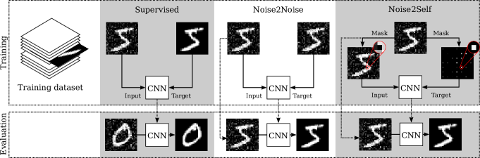
Figure 1: Three training regimes for CNN-based image denoising. Supervised training is performed with noisy and clean images, and the trained CNN is applied to unseen noisy data. Noise2Noise training is performed with pairs of noisy images. Noise2Self training is performed with just noisy images, which are split into input-target pairs. The loss is only computed where target pixels are non-zero. The red inset displays one of these locations. For Noise2Noise and Noise2Self, the trained CNN can be applied to the training data to obtain clean images.

The supervised training scheme has access to a training dataset containing pairs of noisy input and clean target images

$$(\mathrm{\tilde{y}}_{i},\mathrm{y}_{i})\sim(\mathsf{y}+\epsilon,\mathsf{y}),\quad i=1,\ldots,N,$$ (2)

where $\mathsf{y}$ is a random variable taking values in $\mathcal{Y}$ that represents the clean images. The supervised training objective is to find the regression function

$$h^{*}=\operatorname*{arg\,min}_{h}\mathbb{E}_{\mathsf{y},\epsilon}\left[\left\lVert h(\mathsf{y}+\epsilon)-\mathsf{y}\right\rVert_{2}^{2}\right],$$ (3)

that minimizes the expected prediction error [35]. The most common loss function is the pixel-wise mean square error, which we use here. Alternative training losses are also used, such as the L1 loss and perceptual losses [18]. Solving Equation (3) is usually intractable. Therefore, the expectation is estimated by the sample mean over the training dataset, which is minimized over neural networks $f_{\varphi}:\mathcal{Y}\to\mathcal{Y}$ with parameters $\varphi$. The training task is then to find the optimal parameters

$$\hat{\varphi}=\operatorname*{arg\,min}_{\varphi}\sum_{i=1}^{N}\left\lVert f_{\varphi}(\mathrm{\tilde{y}}_{i})-\mathrm{y}_{i}\right\rVert_{2}^{2},$$ (4)

which minimize the loss on the sampled image pairs. The trained network $f_{\hat{\varphi}}$ is applied to unseen noisy images to obtain denoised images, as displayed in Figure 1.

The regression function that minimizes the expected prediction error in Equation (3) is the conditional expectation

$$h^{*}(\mathit{\tilde{y}})=\mathbb{E}\left[\mathsf{y}\mid\mathsf{y}+\epsilon=\mathit{\tilde{y}}\right].$$ (5)

In practice, the trained neural network $f_{\hat{\varphi}}$ does not equal $h^{*}$ and an approximation is obtained.

Noise2Noise training may be applied if no clean images are available, but one can measure independent instances of the noise for each image. The training dataset contains pairs of independent noisy images

$$(\mathrm{y}_{i}+\epsilon_{i},\mathrm{y}_{i}+\delta_{i})\sim(\mathsf{y}+\epsilon,\mathsf{y}+\delta),\quad i=1,\ldots,N,$$ (6)

where the noise $\delta$ is a random variable that is statistically independent of $\epsilon$. The training task is to determine

$$\hat{\varphi}=\operatorname*{arg\,min}_{\varphi}\sum_{i=1}^{N}\left\lVert f_{\varphi}(\mathrm{y}_{i}+\epsilon_{i})-(\mathrm{y}_{i}+\delta_{i})\right\rVert_{2}^{2},$$ (7)

and the trained neural network $f_{\hat{\varphi}}$ approximates

$$h^{*}=\operatorname*{arg\,min}_{h}\mathbb{E}_{\mathsf{y},\epsilon,\delta}\left[\left\lVert h(\mathsf{y}+\epsilon)-(\mathsf{y}+\delta)\right\rVert_{2}^{2}\right].$$ (8)

If the noise $\delta$ is mean-zero, i.e., $\mathbb{E}\left[\delta\right]=0$, the expected prediction error in Equation (8) is minimized by the same regression function $h^{*}$ as in the supervised regime (Equation (5)). In practice, Noise2Noise and supervised training indeed yield trained networks with similar denoising performance.

Noise2Self enables training a neural network denoiser without any additional images. The training dataset contains only noisy images

$$\mathrm{\tilde{y}}_{i}\sim\mathsf{y}+\epsilon,\quad i=1,\ldots,N.$$ (9)

The method depends on the assumption that the noise is element-wise statistically independent and mean-zero, and that the clean images exhibit some spatial correlation.

Noise2Self training uses a masking scheme that ensures that the loss compares two statistically independent images. For simplicity, we describe a simplified version of Noise2Self training, and refer to [20] for a more in-depth explanation. In each training step, the noisy image is split into two sub-images: one sub-image — the target — contains non-adjacent pixels and the other sub-image — the input — contains the remaining surrounding pixels. The network is trained to predict the value of a noisy pixel from its surrounding noisy pixels, as is shown in Figure 1.

The division of pixels between the input and target image is determined by a partition $\mathcal{J}$ of the pixels such that adjacent pixels are in different subsets. We denote by $J\in\mathcal{J}$ the target section, and by $J^{C}$ the input section, where $J^{C}$ denotes the set complement of $J$, containing all pixel locations not contained in $J$. The input and target images $\mathbbm{1}_{J^{C}}\mathrm{\tilde{y}}_{i}$ and $\mathbbm{1}_{J}\mathrm{\tilde{y}}_{i}$ have non-zero pixels only in the input and target section, respectively. Here, $\mathbbm{1}_{J}$ denotes the indicator function such that element-wise multiplication of $\mathbbm{1}_{J}$ with an image retains pixel values in $J$ and sets pixels to zero elsewhere. The training task is to determine the set of network parameters minimizing the training loss

$$\hat{\varphi}=\operatorname*{arg\,min}_{\varphi}\sum_{i=1}^{N}\sum_{J\in\mathcal{J}}\lVert\mathbbm{1}_{J}f_{\varphi}(\mathbbm{1}_{J^{C}}\mathrm{\tilde{y}}_{i})-\mathbbm{1}_{J}\mathrm{\tilde{y}}_{i}\rVert_{2}^{2},$$ (10)

where the loss is only computed on the target sections.

The inference step is performed by the section-wise combined network $g_{\hat{\varphi}}:\mathcal{Y}\to\mathcal{Y}$,

$$g_{\hat{\varphi}}(\mathit{\tilde{y}}):=\sum_{J\in\mathcal{J}}\mathbbm{1}_{J}f_{\hat{\varphi}}(\mathbbm{1}_{J^{C}}\mathit{\tilde{y}}),$$ (11)

that computes the output in each target section by applying the trained network to the input section.

The piecewise-combined network is an approximation of the regression function

$$g^{*}(\mathit{\tilde{y}})=\sum_{J\in\mathcal{J}}\mathbbm{1}_{J}\mathbb{E}[\mathbbm{1}_{J}\mathsf{y}\mid\mathbbm{1}_{J^{C}}\left(\mathsf{y}+\epsilon\right)=\mathbbm{1}_{J^{C}}\mathit{\tilde{y}}].$$ (12)

This regression function computes the conditional expectation of the clean image in each target section using the surrounding noisy pixels.

Although aforementioned methods can produce accurately denoised photographic images in many cases [32, 18, 20], a subclass of these algorithms — Noise2Self in particular — has strong requirements on the element-wise independence of the noise. These requirements do not generally hold for solutions of linear inverse problems, as we discuss next.

II-B Linear inverse problems

We are concerned with inverse problems that are described by the equation

$$\mathbf{A}\mathbf{x}=\mathbf{y},$$ (13)

where $\mathbf{x}\in\mathcal{X}=\mathbb{R}^{n}$ denotes an unknown image that we wish to recover, and $\mathbf{y}\in\mathcal{Y}=\mathbb{R}^{m}$ denotes the indirect measurement. The linear forward operator $\mathbf{A}:\mathbb{R}^{n}\to\mathbb{R}^{m}$ describes the physical model by which the measurement arises from the image $\mathbf{x}$. As in the image denoising setting, these measurements are corrupted by element-wise independent noise $\epsilon$, and we write

$$\mathbf{\tilde{y}} =\mathbf{A}\mathbf{x}+\epsilon.$$ (14)

Although noise in Equation (14) is modeled as an additive term, we note that this model also covers non-additive noise, such as Poisson noise, where the noise term typically depends on the signal intensity.

Reconstruction algorithms approximate the image $\mathbf{x}$ from measured data $\mathbf{y}$. A subclass of these reconstruction algorithms computes a linear operator $\mathbf{R}:\mathcal{Y}\to\mathcal{X}$. Examples of linear reconstruction algorithms include the filtered backprojection algorithm for tomography and Wiener filtering for deconvolution microscopy [11, 1]. We denote the reconstruction from a noisy measurement by

$$\tilde{\mathbf{x}}=\mathbf{R}\mathbf{\tilde{y}}=\mathbf{R}\mathbf{y}+\mathbf{R}\epsilon,$$ (15)

which can contain artifacts unrelated to the measurement noise, e.g., under-sampling artifacts and/or reconstruction artifacts. The reconstruction operator $\mathbf{R}$ may cause elements of the reconstructed noise $\mathbf{R}\epsilon$ to be statistically coupled, even if $\epsilon$ is element-wise independent [13]. That $\mathbf{R}\epsilon$ does not satisfy the element-wise independence property is unavoidable for all but the most trivial cases, since inverse problems are essentially defined by the intricate coupling of the unknown image with its indirect measurement.

This coupling of the noise seriously degrades the effectiveness of the Noise2Self approach, as we will see in Section IV-D. In the next section, we propose a self-supervised method that does take into account the properties of noise in inverse problems.

III Noise2Inverse

In this section, we present the proposed Noise2Inverse method. First, we describe the assumed noise model, and give a general description of the method. In Section III-A, we provide a theoretical explanation how and why the convolutional neural network learns to denoise. Here, we also discuss how these results can guide implementation in practice. In Section III-B, we give a more practical description of the implementation for tomography, and discuss implementation choices with regard to the obtained theoretical results.

Suppose that we wish to examine several unknown images $\mathrm{x}_{1},\ldots,\mathrm{x}_{N}\sim\mathsf{x}$, sampled from some random variable $\mathsf{x}$. We obtain noisy indirect measurements

$$\mathrm{\tilde{y}}_{i}\sim\mathbf{A}\mathrm{x}_{i}+\epsilon,\quad i=1,\ldots,N,$$ (16)

where we assume that the noise $\epsilon$ is element-wise independent and mean-zero conditional on the data, i.e.,

$$\mathbb{E}_{\mathsf{x},\epsilon}\left[\mathbf{A}\mathsf{x}+\epsilon\mid\mathbf{A}\mathsf{x}=\mathrm{y}\right]=\mathrm{y}.$$ (17)

As in Equation (14), we assume the noisy may be non-additive. Our goal is to recover the clean reconstructions that would have been obtained in the absence of noise, i.e., $\mathrm{x}^{*}_{i}=\mathbf{R}\mathrm{y}_{i}$ with $\mathrm{y}_{i}=\mathbf{A}\mathrm{x}_{i},i=1,\ldots,N$.

One approach is to compute noisy reconstructions, and use Noise2Self to remove the noise in the reconstructed images. Given the noisy reconstructions $\mathrm{\tilde{{x}}}_{i}~{}=~{}\mathbf{R}\mathrm{\tilde{y}}_{i},i=1,\ldots,N$, the training task is to determine the network parameters minimizing the training loss

$$\hat{\varphi}=\operatorname*{arg\,min}_{\varphi}\sum_{J\in\mathcal{J}_{x}}\sum_{i=1}^{N}\left\lVert\mathbbm{1}_{J}f_{\varphi}(\mathbbm{1}_{J^{C}}\mathrm{\tilde{{x}}}_{i})-\mathbbm{1}_{J}\mathrm{\tilde{{x}}}_{i}\right\rVert_{2}^{2},$$ (18)

where the target sections are contained in $\mathcal{J}_{x}$, a partition of the pixels of the reconstructed images. As discussed before, however, the noise in the input and target pixels of the reconstructed images are unlikely to be statistically independent.

The key idea of the proposed Noise2Inverse method is that it partitions the data in the measurement domain — where the noise is element-wise independent — but trains the CNN in the reconstruction domain. In each training step, the measured data is partitioned into an input and target component, and a neural network is trained to predict the reconstruction of one from the reconstruction of the other. After training, the neural network is applied to denoise the reconstructions.

The division of measured data between input and target is determined by the collection $\mathcal{J}$ of target sections $J\subset\{1,2,\ldots,m\}$ that represent subsets of the measurement domain $\mathcal{Y}=\mathbb{R}^{m}$. We note that $\mathcal{J}$ can be chosen such that it contains structured subsets of the measurement domain, rather than all subsets. For each target section $J\in\mathcal{J}$, the measurement is split into input and target sub-measurements $\mathrm{\tilde{y}}_{i,J^{C}}$ and $\mathrm{\tilde{y}}_{i,J}$, where $J^{C}$ denotes the set complement of $J$ with respect to $\{1,2,\ldots,m\}$. The input and target sub-reconstructions are computed by linear reconstruction operators $\mathbf{R}_{J}:\mathcal{Y}_{J}\to\mathcal{X}$ that take into account only the measurements in section $J\in\mathcal{J}$. We define

$$\mathrm{\tilde{{x}}}_{i,J^{C}}=\mathbf{R}_{J^{C}}\mathrm{\tilde{y}}_{i,J^{C}}\text{ and }\mathrm{\tilde{{x}}}_{i,J}=\mathbf{R}_{J}\mathrm{\tilde{y}}_{i,J}$$

to be the input and target sub-reconstructions of $\mathrm{\tilde{y}}_{i}$, respectively.

The training task is to determine the parameters

$$\hat{\varphi}=\operatorname*{arg\,min}_{\varphi}\frac{1}{\absolutevalue{\mathcal{J}}}\sum_{J\in\mathcal{J}}\sum_{i=1}^{N}\left\lVert f_{\varphi}(\mathrm{\tilde{{x}}}_{i,J^{C}})-\mathrm{\tilde{{x}}}_{i,J}\right\rVert_{2}^{2},$$ (19)

that best enable the network $f_{\hat{\varphi}}$ to predict the target sub-reconstruction from the complementary input sub-reconstruction.

The final output is computed by the section-wise averaged network, which applies the trained network to each input sub-reconstruction, and computes the average, yielding

$$\mathrm{x}^{*}_{i,\text{out}} =\frac{1}{\absolutevalue{\mathcal{J}}}\sum_{J\in\mathcal{J}}f_{\hat{\varphi}}\left(\mathrm{\tilde{{x}}}_{i,J^{C}}\right).$$ (20)

In the next section, we show why the final result approximates the clean reconstruction.

III-A Theoretical framework

In this section, we embed Noise2Inverse in a theoretical framework that explains why it is an accurate denoising method. In addition, we describe design considerations that enable it to operate successfully.

Below, we show that Noise2Inverse recovers an average clean reconstruction in theory. This result is founded upon Proposition 1, which shows that the expected prediction error is the sum of the variance of the reconstructed noise and the supervised prediction error, which is the expected prediction error that would have obtained if the target reconstructions were noise-free. Hence, the regression function that minimizes the expected prediction error also minimizes the loss with respect to the unknown clean reconstruction. Therefore, it predicts a clean sub-reconstruction when given a noisy sub-reconstruction.

As before, we represent the clean and noisy measurements by the random variables $\mathsf{y}=\mathbf{A}\mathsf{x}$ and $\mathsf{\tilde{y}}=\mathsf{y}+\epsilon$. The input and target sub-reconstructions are represented by random variables $\mathsf{\tilde{x}}_{J^{C}}=\mathbf{R}_{J^{C}}\mathsf{\tilde{y}}_{J^{C}}$ and $\mathsf{\tilde{x}}_{J}=\mathbf{R}_{J}\mathsf{\tilde{y}}_{J}$ for $J\in\mathcal{J}$. In this case, the trained network $f_{\hat{\varphi}}$ obtained in Equation (19) approximates the regression function

$$h^{*} =\operatorname*{arg\,min}_{h}\frac{1}{\absolutevalue{\mathcal{J}}}\sum_{J\in\mathcal{J}}\mathbb{E}_{\mathsf{x},\epsilon}\left\lVert h(\mathsf{\tilde{x}}_{J^{C}})-\mathsf{\tilde{x}}_{J}\right\rVert^{2},$$ (21)

which minimizes the expected prediction error. We randomize the section $J$ as well, representing it by $\mathsf{J}$ taking values uniformly at random in $\mathcal{J}$. The input and target sub-reconstructions become random in $\mathsf{J}$ as well, which is denoted by $\mathsf{\tilde{x}}_{\mathsf{J}^{C}}=\mathbf{R}_{\mathsf{J}^{C}}\mathsf{\tilde{y}}_{\mathsf{J}^{C}}$ and $\mathsf{\tilde{x}}_{\mathsf{J}}=\mathbf{R}_{\mathsf{J}}\mathsf{\tilde{y}}_{\mathsf{J}}$. The expected prediction error then becomes

$$\frac{1}{\absolutevalue{\mathcal{J}}}\sum_{J\in\mathcal{J}}\mathbb{E}_{\mathsf{x},\epsilon}\left\lVert h(\mathsf{\tilde{x}}_{J^{C}})-\mathsf{\tilde{x}}_{J}\right\rVert^{2} =\mathbb{E}_{\mu}\left\lVert h(\mathsf{\tilde{x}}_{\mathsf{J}^{C}})-\mathsf{\tilde{x}}_{\mathsf{J}}\right\rVert^{2},$$

where we replace the average over $J\in\mathcal{J}$ by the expectation with respect to $\mathsf{J}$. We denote with $\mu$ the joint measure of $\mathsf{x},\epsilon$, and $\mathsf{J}$. Define the sub-reconstruction of the clean measurement

$$\mathsf{x^{*}}_{\mathsf{J}} =\mathbf{R}_{\mathsf{J}}\mathsf{y}_{\mathsf{J}},$$ (22)

which describes the clean target reconstruction. Now the expected prediction error can be decomposed into two parts.

Proposition 1 (Expected prediction error decomposition).

Let $\mathsf{\tilde{x}}_{\mathsf{J}},\mathsf{\tilde{x}}_{\mathsf{J}^{C}},\mathsf{x^{*}}_{\mathsf{J}}$, and $\mu$ be as above. Let $\epsilon$ be element-wise independent and satisfy (17). Let $\mathbf{R}_{J}$ be linear for all $J\in\mathcal{J}$. Then, for any measurable function $h:\mathcal{X}\to\mathcal{X}$, we have

$$\mathbb{E}_{\mu}\left\lVert h(\mathsf{\tilde{x}}_{\mathsf{J}^{C}})-\mathsf{\tilde{x}}_{\mathsf{J}}\right\rVert_{2}^{2}=\mathbb{E}_{\mu}\left\lVert h(\mathsf{\tilde{x}}_{\mathsf{J}^{C}})-\mathsf{x^{*}}_{\mathsf{J}}\right\rVert_{2}^{2}\\ +\mathbb{E}_{\mu}\left\lVert\mathsf{x^{*}}_{\mathsf{J}}-\mathsf{\tilde{x}}_{\mathsf{J}}\right\rVert_{2}^{2}.$$ (23)

Proposition 1 states that the expected prediction error can be decomposed into the supervised prediction error, which depends on the choice of $h$, and the variance of the reconstruction noise, which does not depend on $h$. Therefore, when minimizing (23), the function $h$ minimizes the difference between its output and the unknown clean target sub-reconstruction $\mathsf{x^{*}}_{\mathsf{J}}$. Note that the minimization of $h$ occurs with respect to $\mathsf{x^{*}}_{\mathsf{J}}$ instead of the fully sampled reconstruction $\mathbf{x}^{*}$. When the target sections have been chosen such that $\mathbb{E}_{\mathsf{J}}\left[\mathsf{x^{*}}_{\mathsf{J}}\right]=\mathbf{x}^{*}$ holds, however, the difference is minimized.

The supervised prediction error, $\mathbb{E}_{\mu}\lVert h(\mathsf{\tilde{x}}_{\mathsf{J}^{C}})-\mathsf{x^{*}}_{\mathsf{J}}\rVert_{2}^{2}$, is minimized [36] by the regression function

$$h^{*}(\mathit{\tilde{x}}) =\mathbb{E}_{\mu}\left[\mathsf{x^{*}}_{\mathsf{J}}\mid\mathsf{\tilde{x}}_{\mathsf{J}^{C}}=\mathit{\tilde{x}}\right].$$ (24)

The section-wise averaged network, defined in Equation (20), therefore approximates the section-wise average of the regression function, defined by

$$g^{*}(\mathit{\tilde{y}}) =\frac{1}{\absolutevalue{\mathcal{J}}}\sum_{J\in\mathcal{J}}\mathbb{E}_{\mu}\left[\mathsf{x^{*}}_{\mathsf{J}}\mid\mathsf{\tilde{x}}_{\mathsf{J}^{C}}=\mathit{\tilde{x}}_{J^{C}}\right],$$ (25)

where we write $\mathit{\tilde{x}}_{J^{C}}=\mathbf{R}_{J^{C}}\mathit{\tilde{y}}_{J^{C}}$ for $\mathit{\tilde{y}}\in\mathcal{Y}$ and $J\in\mathcal{J}$.

Using these results, we can explain why the section-wise average obtains a denoised output. A noisy sub-reconstruction can be explained by different values of the clean reconstruction $\mathsf{x^{*}}$. The expectation $\mathbb{E}_{\mu}\left[\mathsf{x^{*}}_{\mathsf{J}}\mid\mathsf{\tilde{x}}_{\mathsf{J}^{C}}=\mathit{\tilde{x}}_{J^{C}}\right]$ is the mean of noiseless reconstructed images consistent with the observed noisy reconstruction $\mathit{\tilde{x}}_{J^{C}}$. Equation (24) therefore predicts that our method produces denoised images. In fact, our method computes the mean over all clean sub-reconstructions indicated by $J\in\mathcal{J}$.

The obtained results may be used to guide implementation in practice. Equation (25) explains how to choose subsets $\mathcal{J}$. First of all, the mean of the clean sub-reconstructions $\nicefrac{{1}}{{\absolutevalue{\mathcal{J}}}}\sum_{J\in\mathcal{J}}\mathsf{x^{*}}_{J}$ must resemble the desired clean image. This can be achieved by choosing $\mathcal{J}$ to be a partition of $\{1,\ldots,m\}$, or, by choosing $\mathcal{J}$ such that each measured data point is contained in the same number of overlapping subsets $J\in\mathcal{J}$. Not doing so introduces a systematic bias into the reconstruction.

Second, the sub-reconstructions should be homogeneously informative throughout the image. If the sub-reconstructions are very different, or contain limited information about large parts of the image, then many dissimilar clean images are consistent with the observed noisy reconstruction, and the average over all these images will become blurred.

We note that $\mathsf{x^{*}}$ denotes the clean reconstruction, rather than the unknown image. This has two consequences. First, the theory predicts that artifacts that are unrelated to the measurement noise, e.g. under-sampling artifacts and reconstruction artifacts, will not be removed by the proposed network. Second, if the reconstruction method also performs denoising operations, for instance by blurring, then the result of our method might become blurred. The same effect might occur when a non-linear reconstruction method is used, for which Proposition 1 does not generally hold. In this case, the regression function averages the bias introduced by the non-linear reconstruction of the noise. In the next section, we use the considerations discussed above to devise an approach for computed tomography.

III-B Noise2Inverse for computed tomography

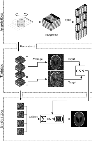
Figure 2: Noise2Inverse for computed tomography. First, 3D parallel-beam tomography obtains a stack of noisy sinograms by integrating over parallel lines at several angles. Next, the stack of sinograms is split along the angular axis. Then, the split sinograms are reconstructed to act as training dataset. During training, a dynamic subset of slices is averaged to form the input; the target is the average of the remaining slices. To obtain a low-noise result, the trained CNN is applied to all arrangements of input slices and averaged.

In this section, we describe our implementation of Noise2Inverse for 3D parallel-beam tomography, and discuss how the implementation relates to the theoretical considerations discussed before.

The 3D parallel-beam tomography problem may be considered as a stack of 2D parallel-beam problems. In 2D parallel-beam tomography, a parallel X-ray beam penetrates an object, after which it is measured on a line detector. The line detector rotates around the object while capturing the intensity of the attenuated X-ray beam, as illustrated in the top panel of Figure 2.

In practice, a finite number of $N_{\theta}$ projections are acquired on a line grid of $N_{p}$ detector elements at fixed angular intervals. Hence, the projection data can be described by a vector $\mathbf{\tilde{y}}\in\mathcal{Y}=\mathbb{R}^{m},m=N_{\theta}\times N_{p}$, which is known as the sinogram. Likewise, the two-dimensional imaged object is represented by a vector $\mathbf{x}\in\mathcal{X}=\mathbb{R}^{n},n=N_{x}^{2}$. We can formulate 2D parallel-beam tomography as a discrete linear inverse problem, where $\mathbf{A}=(a_{ij})$ is an $m\times n$ matrix such that $a_{ij}$ represents the contribution of object pixel $j$ to detector pixel $i$. In 3D tomography, a sequence of 2D projection images of the 3D structure is acquired, which may be converted to a stack of 2D sinograms.

The imaged object can be recovered from the sinogram by a reconstruction algorithm, such as the filtered back-projection algorithm (FBP) [11]. FBP is an example of a linear operator that couples the measured noise in the reconstruction, as described in Equation (15). In addition, it is typically fast to compute, although its reconstructions tend to be noisy [15].

The Noise2Inverse method is well-suited to denoise this kind of problem. Suppose we have obtained a stack of 2D noisy sinograms $\mathrm{\tilde{y}}_{1},\mathrm{\tilde{y}}_{2},\ldots,\mathrm{\tilde{y}}_{N}$, acquired from a range of $N_{\theta}$ equally-spaced angles $\theta_{1},\theta_{2},\ldots,\theta_{N_{\theta}}$. Our approach follows the following steps.

First, we split each sinogram $\mathrm{\tilde{y}}_{i}$ into $K$ sub-sinograms $\mathrm{\tilde{y}}_{i,1},\ldots,\mathrm{\tilde{y}}_{i,K}$ such that each sub-sinogram $\mathrm{\tilde{y}}_{i,j}$ contains pixels from every $K$th angle $\theta_{j},\theta_{j+K},\theta_{j+2K},\ldots,\theta_{j+N_{\theta}-K}$. The number of splits $K$ is a hyper-parameter of the method.

Using the FBP algorithm, we compute sub-reconstructions

$$\mathrm{\tilde{{x}}}_{i,j}=\mathbf{R}_{j}(\mathrm{\tilde{y}}_{i,j}),\quad j=1,\ldots,K.$$ (26)

For training, the division of the sub-reconstructions over the input and target is determined by a collection $\mathcal{J}$, which contains subsets $J\subset\{1,\ldots,K\}$. For $J\subset\{1,\ldots,K\}$, we define the mean sub-reconstruction as

$$\mathrm{\tilde{{x}}}_{i,J}=\frac{1}{\absolutevalue{J}}\sum_{j\in J}\mathrm{\tilde{{x}}}_{i,j}.$$ (27)

As before, training of the neural network $f_{\varphi}$ aims to find

$$\hat{\varphi}=\operatorname*{arg\,min}_{\varphi}\sum_{i=1}^{N}\sum_{J\in\mathcal{J}}\lVert f_{\varphi}\left(\mathrm{\tilde{{x}}}_{i,J^{C}}\right)-\mathrm{\tilde{{x}}}_{i,j}\rVert_{2}^{2}.$$ (28)

The final output, $\mathrm{x}^{*}_{i,\text{out}}$, is computed slice by slice by section-wise averaging of the output of the trained network

$$\mathrm{x}^{*}_{i,\text{out}} =\frac{1}{\absolutevalue{\mathcal{J}}}\sum_{J\in\mathcal{J}}f_{\hat{\varphi}}\left(\mathrm{\tilde{{x}}}_{i,J^{C}}\right).$$

In this paper, we identify two training strategies specifying $\mathcal{J}$:

X:1

Using this strategy, the input is the mean of $K-1$ sub-reconstructions, and the target is the remaining sub-reconstruction, i.e.,

$$\mathcal{J}_{X:1}=\{\{1\},\{2\},\ldots,\{K\}\}.$$ (29)

1:X

This is the reverse of the previous strategy: the input is a single sub-reconstruction, and the target is the mean of the remaining sub-reconstructions, i.e.,

$$\mathcal{J}_{1:X} =\{J^{C}\mid J\in\mathcal{J}_{X:1}\}.$$ (30)

In the 1:X strategy, the input is noisier than the target image, which corresponds to supervised training, where the quality of the target images is usually higher than the input images. The opposite is the case for the X:1 strategy, which corresponds more closely to Noise2Self denoising in its distribution of data between input and target, where more pixels are used to compute the input than to compute the target images. Note that other splits are possible, but we focus on these two strategies because they represent two extremes in the trade-off between input quality and target quality.

Our implementation of Noise2Inverse for tomography is consistent with the theoretical considerations discussed in the previous section. In both strategies, we prevent biasing the reconstructions, by ensuring that each projection angle occurs in reconstructions at the same rate. In fact, a property of FBP is that the full reconstruction is the mean of the sub-reconstructions. In theory, this means that training converges to the conditional expectation of the full clean FBP reconstruction. Furthermore, we use every $K$th projection angle to compute the reconstructions. This ensures that the reconstructions are homogeneously informative throughout the image, and we prevent missing wedge artifacts, which occur when adjacent projection angles are used [37]. In addition, we use the FBP algorithm with the Ram-Lak filter[11], which does not blur the reconstructions to remove noise. Finally, we remark that our method is not geometry-specific, and can also be applied to non-parallel geometries, as is demonstrated in Section IV-C. In the next section, we describe the performance of this implementation in practice.

IV Results

We performed several experiments on tomographic reconstruction problems. These experiments were performed with the aim of assessing the performance of the proposed Noise2Inverse method, determining the suitability of Noise2Self denoising for tomographic images, and analyzing the impact of hyper-parameters on the performance of Noise2Inverse.

Comparison to denoising techniques Noise2Inverse is compared to tomographic reconstruction algorithms, an image denoising method, and an unsupervised deep learning method in Sections IV-A, IV-B, and IV-C. These sections describe a quantitative evaluation on simulated tomographic data, medical CT data with simulated noise, and a qualitative evaluation on an existing experimental dataset.

Noise2Self on tomographic images The experiments in Section IV-D investigate a transfer of Noise2Self denoising to inverse problems. The Noise2Self method was evaluated on two datasets: one dataset with noise common to tomographic reconstructions and one with similar but element-wise independent noise. In addition, Noise2Inverse was compared to several variations of Noise2Self.

Hyper-parameters In Section IV-F, the impact on the reconstruction quality of several variables was investigated, specifically, the number of projection angles $N_{\theta}$, the number of splits $K$, the training strategy $\mathcal{J}$, and the neural network architecture. In addition, we analyze the generalization performance of the Noise2Inverse approach by training on progressively smaller subsets of the training dataset.

We first describe the simulated tomographic dataset and our implementation of Noise2Inverse. Both are used throughout the experiments.

Simulated data A cylindrical foam phantom was generated containing 100,000 randomly-placed non-overlapping bubbles. Analytical projection images of the phantom were computed using the open-source foam_ct_phantom package [10]. The value of each detector pixel was calculated by taking the average projection value of four equally-spaced rays through the pixel. Projection images were acquired from $1024$ equally spaced angles.

The projection images of the foam dataset were corrupted with various levels of Poisson noise. The noise was varied by altering the average absorption of the sample $\alpha$ and the incident photon count per pixel $I_{0}$. The average absorption of the sample was calculated as the mean of the vector $1-e^{-\mathbf{y}_{i}}$ for positions $i$ where $\mathbf{y}_{i}$ was non-zero, and it was adjusted by modifying the intensity of the sinogram. The pixels in the noisy projections where sampled from $\mathsf{\tilde{p}}$, which for clean pixel value $\mathrm{p}$ was distributed as

$$I_{0}e^{-\mathsf{\tilde{p}}}\sim\text{Poisson}\left(I_{0}e^{-\mathrm{p}}\right).$$

i.e., a Poisson distribution on the pre-log raw data. Depending on the photon count and attenuation of the object, this type of noise is mean-zero conditional on the clean projections, as described in Equation (17).

FBP reconstructions were computed on a $512^{3}$ voxel grid with the Ram-Lak filter using the ASTRA toolbox [38]. On this grid, the radius of the random spheres ranged between $1.5$ and $51$ voxels. A reconstruction of the central slice of the foam phantom can be found in Figure 3, along with reconstructions of the noisy projection datasets.

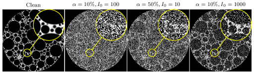
Figure 3: Displays of the clean reconstruction (left) and low-dose reconstructions of the central slice of the foam phantom. Both $\alpha$, the absorption of the phantom and $I_{0}$, the initial photon count per pixel, were varied. The yellow insets show an enlarged view of the reconstructions.

Noise2Inverse We describe the Noise2Inverse implementation in terms of neural network architecture and training procedure.

The principal network architecture used throughout the experiments was the mixed-scale dense (MS-D) network [39], of which we used the open-source msd_pytorch implementation [40]. The MS-D network has 100 single-channel intermediate layers, and the convolutions in layer $i$ are dilated by $d_{i}=1+(i\mod 10)$. With 45,652 trainable network parameters, the MS-D architecture has considerably fewer parameters than comparable network architectures, reducing the risk of overfitting to the noise. The MS-D architecture is compared with other architectures in Section IV-F.

The networks were trained for $100$ epochs using the ADAM algorithm [41] with a mini-batch size of $12$ and a learning rate of $10^{-3}$.

IV-A Simulation study

In this section, Noise2Inverse is compared to two conventional iterative reconstruction techniques: the simultaneous iterative reconstruction technique (SIRT) [42] and Total-Variation Minimization (TV-MIN) [43]. In addition, we compare to the BM3D image denoising algorithm [33], the Deep Image Prior[26], and to supervised training. The reconstruction quality of these methods is assessed on a simulated foam phantom dataset with various noise profiles.

For Noise2Inverse, we used the X:1 training strategy with $K=4$ splits. We show that this is a robust choice in Section IV-F.

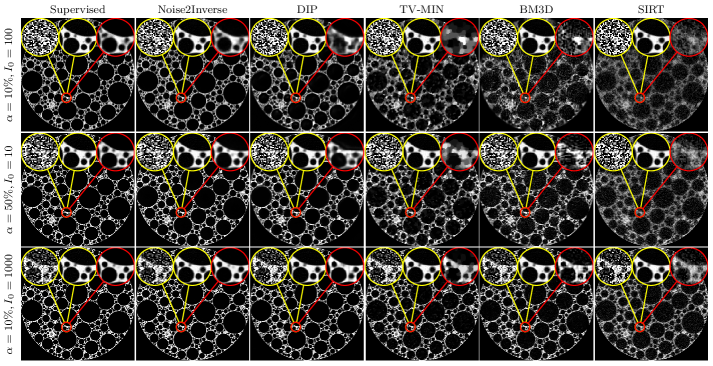
Figure 4: Results of supervised training, Noise2Inverse, Deep Image Prior (DIP), TV-MIN, BM3D, and SIRT on simulated foam phantoms with varying absorption $\alpha$ and photon count $I_{0}$. Results are shown on the central slice. The insets display the noisy and clean reconstructions (yellow) and the algorithm output (red).

Iterative reconstruction The hyper-parameters of SIRT and TV-MIN were tuned using the usually unavailable clean reconstructions. Therefore, the results of SIRT and TV-MIN might be better than what is achievable in practice, but they serve as a useful reference for comparison to Noise2Inverse. SIRT has no explicit hyper-parameters, but its iterative nature can be exploited for regularization: early stopping of the algorithm can attenuate high-frequency noise in the reconstructed image [42]. We selected the number of iterations (with a maximum of 1000) with the lowest Peak Signal to Noise Ratio (PSNR) on the central slice with respect to the clean reconstruction.

The FISTA algorithm [43] was used to calculate the TV-MIN reconstruction. TV-MIN has a regularization parameter $\lambda$ that effectively penalizes steps in the gray value of the reconstructed image. As with SIRT, we selected the optimal number of iterations (with a maximum of 500) based on the PSNR of the central slice with respect to the clean reconstruction, and the value of the $\lambda$ parameter maximizing the PSNR was determined using the Nelder-Mead method [44].

BM3D We used the BM3D implementation described in [45]. The BM3D algorithm was applied to the noisy FBP reconstructions and provided with the standard deviation of the noise, which was calculated from the difference image between the noisy and clean FBP reconstruction. The addition of a prewhitening step can improve denoising performance [46], but was not included as its computation becomes infeasible for large image sizes.

Supervised A separate training dataset was created to train MS-D networks with a supervised training approach. Here, the input and target images were noisy and clean reconstructions, respectively. The training parameters for supervised training — learning rate, batch size, network architecture — were exactly the same as for the Noise2Inverse network.

Deep Image Prior We used the Deep Image Prior implementation from [26]. The quality of the result can be improved by adding noise to the input and by employing an exponentially decaying average of recent iterations [27]. We used both techniques. To maximize the PSNR with respect to the ground truth, the training is stopped early with a maximum of $10000$ iterations, and the $\sigma$ parameter of the input noise is optimized using a line search.

TABLE I: On the full volume and on the central slice: comparison of PSNR and SSIM metrics for SIRT, TV-MIN, BM3D, Deep Image Prior, Noise2Inverse, and a supervised CNN at several noise profiles. Bold font is used to emphasize the best metrics, excluding supervised training, which serves as an oracle case for comparison.

			Full Volume		Central slice
			PSNR	SSIM	PSNR	SSIM
$\alpha$	$I_{0}$	Method
10%	100	Supervised	20.01	0.83	20.02	0.80
		Noise2Inverse	19.71	0.78	19.63	0.74
		Deep Image Prior			17.98	0.59
		TV-MIN	16.89	0.46	16.78	0.40
		BM3D	14.79	0.38	14.81	0.33
		SIRT	15.56	0.36	15.54	0.32
50%	10	Supervised	21.77	0.86	21.71	0.83
		Noise2Inverse	21.66	0.79	21.62	0.75
		Deep Image Prior			19.75	0.67
		TV-MIN	18.08	0.53	17.99	0.48
		BM3D	16.65	0.49	16.74	0.45
		SIRT	16.53	0.42	16.50	0.37
10%	1000	Supervised	26.55	0.91	26.50	0.88
		Noise2Inverse	26.25	0.89	26.24	0.87
		Deep Image Prior			24.03	0.86
		TV-MIN	21.24	0.68	21.24	0.61
		BM3D	21.14	0.69	21.11	0.65
		SIRT	18.84	0.53	18.82	0.48

Metrics and evaluation The output of each method was compared to the clean FBP reconstruction using two metrics: the structural similarity index (SSIM) [47] and the Peak Signal to Noise Ratio (PSNR). Because the reconstructed images did not fall in the $[0,1]$ range, these metrics were computed with a data range that was determined by the minimum and maximum intensity of the clean reconstructed images. The metrics were calculated on the convex hull surrounding the object, which diminishes the importance of the background image quality. Due to the computational demands of deep image prior, we compute metrics on a single slice of the reconstruction rather than on the whole volume.

The top row of Figure 4 displays the output of Noise2Inverse for the central slice of the three simulated datasets. Denoising these datasets is challenging, as can be seen when comparing with SIRT and TV-MIN: these algorithms fail to recover several fine details. In contrast, our method achieves a much improved visual impression on all three datasets. As can be seen in Table I, the PSNR and SSIM metrics of the Noise2Inverse method are considerably higher. The supervised network attains the best metrics, although by a slight margin compared to the Noise2Inverse method.

IV-B Medical CT

To assess the quality of reconstruction on medical data, we evaluate our method on simulated data from human abdomen CT scans from the low-dose CT Grand Challenge dataset [3]. This dataset contains full-dose reconstructions of 10 patients, consisting of a total of $2378$ slices of $512\times 512$ pixels. Following [48], sinograms were computed from these reconstructions by projecting onto a fan-beam geometry. Noise was applied, corresponding to a photon count of $10,000$ incident photons per pixel. Reconstructions are shown in Figure 5.

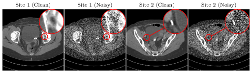
Figure 5: Original high-dose reconstructions of low-dose CT grand challenge (clean) and reconstructions with simulated noise (noisy).

We compare the same methods as before. The dataset was split into a training dataset, consisting of nine patients, and a test set, containing the remaining patient. Both Noise2Inverse and the supervised CNN were trained on the training set. The optimal hyperparameters for SIRT, TV-MIN, and BM3D were determined on the training set. The Deep Image Prior, including its hyperparameters, was directly optimized with respect to the slices displayed in Figure 6. Metrics were calculated on the full volume of the test patient, and on the top displayed slice in Figure 6.

Results are shown in Figure 6 and Table II. The Noise2Inverse method achieves similar results to TV-MIN, but without the staircasing artifacts. The difference between the methods is smaller in this experiment. For the SSIM metric, this is likely due to the low contrast of structures of interest compared to the full intensity range of the reconstructions. In general, compared to previous experiments, the noise has significantly lower intensity, and many different objects structures are present, each of which must be learned by the neural network.

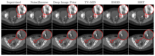
Figure 6: Results of supervised training, Noise2Inverse, Deep Image Prior, TV-MIN, BM3D, and SIRT on Low-dose CT grand challenge data with simulated noise. The red insets display the algorithm output.

TABLE II: Medical data: comparison of PSNR and SSIM metrics for SIRT, TV-MIN, BM3D, Deep Image Prior, a supervised CNN, and Noise2Inverse. Bold font is used to emphasize the best metrics, excluding supervised training, which serves as an oracle case for comparison.

	Full volume		Single slice
	PSNR	SSIM	PSNR	SSIM
Method
Supervised	46.34	0.99	46.29	0.99
Noise2Inverse	45.06	0.99	45.46	0.99
TV-MIN	44.91	0.99	45.65	0.98
Deep Image Prior			44.57	0.98
BM3D	43.84	0.99	43.97	0.98
SIRT	39.87	0.97	40.61	0.95

IV-C Experimental data

The Noise2Inverse method was compared to SIRT and TV-MIN on an existing real-world experimental dataset from TomoBank [49]. The dataset, Dorthe_F_002, was acquired at the Advanced Photon Source at Argonne National Laboratory, and contained $900$ noisy projection images of $960\times 600$ pixels depicting a cylinder of glass beads that was scanned at experimental conditions designed to capture the dynamics of fast evolving samples. At $6$ milliseconds per projection image, the exposure time was therefore much shorter than what is required for low-noise data acquisition [49]. The data was pre-processed with the TomoPy software package [50] and reconstructed with FBP[38], resulting in $900$ 2D slices of $960\times 960$ pixels. We stress that no low-noise projection images were available.

For Noise2Inverse, an MS-D network was trained with the X:1 strategy and $4$ splits for $100$ epochs. The best parameter settings for SIRT and TV-MIN were determined by visual inspection. For SIRT, the best reconstruction was chosen from $1000$ iterations on the central slice. For TV-MIN, the number of iterations was fixed at $500$, and the optimal value of the regularization parameter was chosen from several values regularly spaced on an exponential grid. For BM3D, the best image was chosen from various values of the standard deviation parameter. We have omitted the Deep Image Prior since there was no ground truth with respect to which to perform early stopping.

After initial reconstructions, we found that the reported value of the center of rotation offset — $4.5$ pixels from center — yielded unsatisfactory results. The reconstructions in Figure 7 were computed with a center of rotation that was shifted by $8.9$ pixels. Results are shown for the central slice of the reconstructed volume. The FBP and SIRT reconstructions exhibit severe noise. The TV-MIN reconstruction improves on the level of noise, but contains stepping artifacts that reduce the effective resolution. Our method is able to remove the noise while retaining the finer structure of the image.

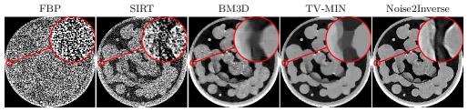
Figure 7: Reconstructions of cylinder containing glass beads [49] using: FBP, SIRT, BM3D, TV-MIN, and the proposed Noise2Inverse method. The red insets show an enlarged view of the algorithm output.

IV-D Self-supervised image denoising for tomography

The performance of Noise2Self on tomographic images was evaluated in two experiments. The first experiment tested the element-wise independence requirement, by evaluating Noise2Self on images corrupted by element-wise independent noise and on images reconstructed from noisy projection data. The second experiment was a comparison of Noise2Inverse to Noise2Self, including variations of Noise2Self applied to projection and sinogram images. We first describe the Noise2Self implementation.

Noise2Self The original implementation of Noise2Self [20] was used, which obtains better performance than the simplified scheme discussed in Section II-A. The training procedure was the same as for Noise2Inverse: an MS-D network was trained for 100 epochs as described at the beginning of Section IV.

Tomographic versus photographic noise Noise2Self was applied to images with coupled reconstructed noise and to similar but element-wise independent noise. In these experiments, the same foam phantom was used as before, and Gaussian noise was used throughout the comparison to strictly compare the independence properties of the noise. First, we confirmed that Noise2Self obtained denoised images when the noise satisfied the element-wise independence property. In this first case, a clean reconstruction was computed on a $512^{3}$ voxel grid, and independent and identically distributed (i.i.d.) Gaussian noise was added to the reconstructed images. The PSNR of the noisy volume with respect to the clean reconstruction was $11.06$. Then, Noise2Self was applied to obtain a denoised volume with significantly improved PSNR of $25.23$. This process is displayed in the top row of Figure 8.

Next, we investigated how Noise2Self performed on coupled reconstructed noise. In this case, i.i.d. Gaussian noise was added to the projection images, and a reconstruction was computed afterwards. The PSNR of this noisy reconstruction with respect to the clean reconstruction was $11.59$. When Noise2Self was applied to the noisy reconstructed volume, it obtained a PSNR of $16.14$, which is only half of the improvement that it obtained in the first case. This process is displayed in the bottom row of Figure 8.

The results displayed in Figure 8 demonstrate that the performance of Noise2Self is substantially degraded when the noise is not element-wise independent. Even though the starting PSNR in the bottom row is slightly higher, the PSNR improvement is only half of the top row. In the top row, the validation error continued to improve for 100 epochs, whereas in the bottom row, training started to overfit to the noise within the first 10 epochs of training, which could be caused by the statistical dependence between the input and target images.

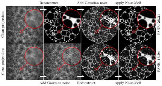
Figure 8: The effect of element-wise independence of the noise on the Noise2Self method. In the top row, Gaussian noise is added to a reconstruction, and Noise2Self is applied to remove it. In the bottom row, Gaussian noise is added to the projections before reconstruction, resulting in a reconstructed image with similar but coupled noise. Noise2Self achieves lower PSNR in the bottom row than in the top row.

Noise2Self on sinogram and projections To mitigate the effect of coupled noise, Noise2Self was also applied to images that do satisfy the pixel-wise independence property: the projection images and sinograms. In these cases, Noise2Self was first applied to denoise the raw images, and reconstructions were computed from the denoised projection images or sinograms.

As can be seen in Figure 9, the variations of Noise2Self did improve results, but not beyond Noise2Inverse. Although applying Noise2Self on the projection and sinogram images did accurately denoise the raw images, the resulting reconstructions of these denoised images exhibited some blurring (projections) and streaks (sinograms). As displayed in Table III, the Noise2Self-based method with the best metrics, Noise2Self on sinograms, obtains PSNR on par with TV-MIN and SSIM worse than TV-MIN, see Table I.

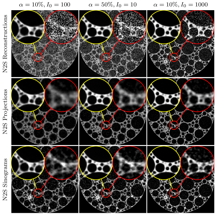
Figure 9: From top to bottom, results on the central slice of the foam phantom of Noise2Self applied to reconstructed, projection, and sinogram images. For comparison, the insets show the output of Noise2Inverse (yellow) and Noise2Self (red).

TABLE III: Comparison of PSNR and SSIM metrics for Noise2Self on reconstruction, projection, and sinogram images.

Absorption	$I_{0}$	Method	PSNR	SSIM
10%	100	N2S Reconstructions	6.37	0.27
		N2S Projections	16.43	0.44
		N2S Sinograms	16.98	0.45
		Noise2Inverse	19.71	0.78
50%	10	N2S Reconstructions	9.12	0.20
		N2S Projections	17.49	0.49
		N2S Sinograms	18.06	0.51
		Noise2Inverse	21.66	0.79
10%	1000	N2S Reconstructions	15.39	0.50
		N2S Projections	19.57	0.62
		N2S Sinograms	20.62	0.60
		Noise2Inverse	26.25	0.89

IV-E Noise2Inverse and missing wedge artifacts

The quality of tomographic reconstructions may be degraded due to artifacts other than measurements noise, such as missing wedge artifacts. These artifacts arise when projection data is acquired along an arc spanning less than 180°. The theoretical results in Section III-A predict that Noise2Inverse preserves these artifacts.

To test this prediction, we apply Noise2Inverse to a foam dataset where the reconstructions are computed from 400 projection images along an arc of approximately 60°. Noise is applied consistent with an absorption of $10\%$ and an incident photon count of $1000$ photons per pixel. As can be seen in Figure 10, Noise2Inverse accurately denoises the reconstructed image, but leaves the missing wedge artifacts intact.

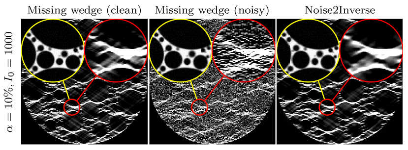
Figure 10: Noise2Inverse applied to a noisy dataset with missing wedge artifacts. The red and yellow insets show an enlarged view of the output and ground-truth, respectively.

IV-F Hyper-parameters

We analyzed the influence of the number of splits, training strategy, number of projection angles, and neural network architecture on the effectiveness of Noise2Inverse. In addition, we tested the generalization by training on subsets of the data.

The same foam phantom was used, and noisy projection data were acquired from $512$, $1024$, and $2048$ angles, of which the first and last acquisitions were under-sampling and over-sampling the projection angles, respectively. For each dataset, the total number of incident photons remained constant: we used $I_{0}=400,200,100$ for $N_{\theta}=512,1024,2048$, respectively. The average absorption was $23\%$, which is the default value of the foam_ct_phantom package.

Splits and strategy The performance of the Noise2Inverse method was evaluated with a number of splits $K=2,4,8,16,32$, and with strategies X:1 and 1:X, see Equations (29) and (30). These experiments were performed with MS-D networks, which were trained for 100 epochs, and used the same training procedure as before.

The PSNR metrics are displayed in Figure 11. The figure shows that the X:1 strategy yields considerably better results than the 1:X strategy, except for $K=2$, where they are equivalent. Setting the number of splits to $K=2$ yields good results across the board, but the PSNR can be improved by setting $K$ to $4$ or $8$, if the projection angles are not under-sampled. In general, the figure shows that increasing the number of acquired projection images can improve reconstruction quality without increasing the photon count. On the other hand, we note that reducing the number of projection images further can reduce the reconstruction quality as the artifacts arising from undersampling are not removed by the neural network.

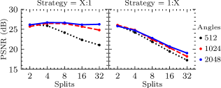
Figure 11: The PSNR metric for the Noise2Inverse method with the MS-D network applied on the foam phantom with varying number of splits, angles, and varying input-target splitting strategies. The X:1 strategy attains higher PSNR than the 1:X strategy.

Neural network architectures We compared three neural network architectures: the U-Net [51], DnCNN [32], and the previously described MS-D [39] network architectures, all of which were implemented in PyTorch [52].

The U-net is based on a widely available open source implementation, which is a mix of the architectures described in [53, 51]. Like [51], the images are down-sampled four times using $2\times 2$ max-pooling, the “up-convolutions” have trainable parameters, and the convolutions have $3\times 3$ kernels. Like [53], this implementation uses batch normalization before each ReLU, the smallest image layers are 512 channels instead of 1024 channels, and zero-padding is used instead of reflection-padding. The resulting network has 14,787,777 trainable network parameters.

We used the DnCNN implementation from [20] with a depth of 20 layers, which is advised for non-Gaussian denoising [32]. The resulting network has 667,008 trainable network parameters.

The previous experiment was repeated on the dataset containing 1024 projection images. The networks were trained for 100 epochs, and used the same training procedure as before. The results are displayed in Figure 12. The figure shows that the U-net achieved overall highest performance using the X:1 strategy with $4$ splits. In addition, the effect of the number of splits $K$ is roughly the same across strategies and network architectures, except for U-net. In fact, the PSNR metric of the U-Net with the 1:X strategy initially increases when $K$ is increased, which might be due to the large network architecture and number of parameters compared to the other two neural network architectures. Nonetheless, the X:1 strategy consistently attains higher PSNR than the 1:X for the U-net as well. We note that the U-Nets performed worse than the other networks with 2 splits, which suggests that training might have overfit the noise.

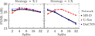
Figure 12: Comparison of the PSNR metric. The MS-D, U-Net, and DnCNN networks were trained for 100 epochs on the foam phantom with 1024 projection angles.

Overfitting We tested if the networks overfit the noise when trained for a long time. All three networks were trained for $1000$ epochs using the X:1 strategy and $K=4$ on the same foam dataset with 1024 projection angles. The resulting PSNR on the central slice as training progressed is displayed in Figure 13. The figure shows that U-Net and DnCNN started to fit the noise, whereas the PSNR of the MS-D network continued to increase. This matches earlier results on overfitting [10, 39, 54]. If the training dataset had been larger, these effects could have been less pronounced.

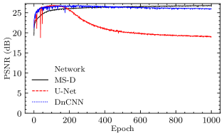
Figure 13: The PSNR on the central slice as training progressed. A U-Net, DnCNN, and MS-D network were trained with the X:1 strategy and number of splits $K=4$ for 1000 epochs on the foam phantom reconstructed from 1024 projection angles.

Generalization We tested whether the network could be trained on fewer data samples and generalize to unseen data. We used the 1024-angle foam dataset, the MS-D network, 4 splits, and the X:1 strategy. The network was trained on the first 4, 8, 16, 32, 64, 128, and 256 slices of the data. We report PSNR metrics on this training set and on the remaining slices, which we refer to as the test set. The number of epochs was corrected for the smaller dataset size, such that all networks were trained for the same number of iterations. When the training set exceeds 32 slices, the PSNR on the training and test set is comparable, as can be seen in Figure 14.

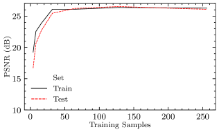
Figure 14: An MS-D network was trained on subsets of the data. The PSNR on the training set (black) and test set (remaining data; red) are displayed.

V Discussion

The results show that the proposed Noise2Inverse method outperforms conventional reconstruction algorithms SIRT and TV-MIN by a large margin as measured in PSNR and SSIM. This improvement is accomplished despite optimizing the hyper-parameters of SIRT and TV-MIN on the clean reconstruction and without likewise optimizing the Noise2Inverse hyper-parameters. In addition, Noise2Inverse is able to significantly reduce noise in challenging real-world experimental data, improving on the visual impression obtained by SIRT and TV-MIN.

Extending the Noise2Self framework[20], we describe a general framework for denoising linear image reconstructions that provides a theoretical rationale for the success of our method. The framework shows that clean reconstructions may be recovered from noisy measurements without observing clean measurements, under the common assumption that the measured noise is element-wise independent and mean-zero. We remark that in low-noise situations, the trained network does not introduce additional artifacts in its output, as predicted by the theory.

We now focus on the comparison between the proposed Noise2Inverse approach and the existing Noise2Noise and Noise2Self approaches. As in Noise2Noise, the network is presented with two noisy images during training. In Noise2Inverse, however, these images are sub-sampled reconstructions, and since the artifacts arising from sub-sampling the data are correlated, the input and target images are not statistically independent — although the reconstructed noise in these images is statistically independent. Therefore, our results fall outside of the Noise2Noise framework. As in Noise2Self, Noise2Inverse trains a denoiser from unpaired measurements. The key difference is that the noise is element-wise independent in the measurement domain, rather than in the reconstruction domain, where denoising takes place. Therefore, the results from [20] do not carry over to the inverse problems setting. However, we are able to prove Proposition 1 using essentially similar arguments to those in [20].

The framework points the way to new applications of Noise2Inverse to linear image reconstruction methods. The implementation of Noise2Inverse for tomography shows that several aspects are worth considering. If reconstruction artifacts arise in the absence of noise, they will be preserved. In addition, if the reconstruction algorithm filters the noise at the expense of resolution, this will cause blurring in the output of our method. Moreover, splitting the measurement uniformly can avoid biasing the output of the method towards a particular subset of the measured data. Finally, the performance of the neural network can be improved by ensuring that the sub-reconstructions are homogeneously informative throughout the image.

Noise2Inverse is well-suited to imaging modalities that permit trading acquisition speed for measurement noise, as it aims to remove measurement noise but does not remove artifacts resulting from under-sampling, Whether this trade-off is possible, depends on the specifics of the imaging modality. Tomographic acquisition, for instance, permits acquiring the same number of projection images by lowering the exposure time at the cost of increased noise [3]. Magnetic Resonance Imaging (MRI), on the other hand, is usually accelerated by reducing the number of measurements, rather than by acquiring noisier measurements [55]. Examples of imaging modalities that permit trading speed for noise include ultrasound imaging [4], deconvolution microscopy [1], and X-ray holography [7].

The comparison of Noise2Inverse with Noise2Self demonstrates that the success of our method depends not only on considerations of statistical independence, but also on taking account of the physical forward model. Regarding statistical independence, we have demonstrated that a straightforward application of Noise2Self fails on noisy tomographic reconstructions due to coupling of the noise. Regarding the forward model, we have investigated a two-step approach, where Noise2Self is applied to projection or sinogram images — which do satisfy the element-wise independence requirement — before reconstructing. This approach performs worse than TV-MIN and Noise2Inverse in terms of visual impression and quality metrics. This matches earlier results [16], and could result from the fact that the consistency of the projection and sinogram images with respect to the forward operator is not necessarily preserved. These results suggest that taking into account the properties of the inverse problem — as Noise2Inverse does — significantly improves the quality of the reconstruction.

Several variables affect the performance of Noise2Inverse. Most importantly, the training strategy that reconstructs the input images from at least as many projection angles as the target images — the X:1 strategy — yields better results than vice versa. This conclusion holds regardless of network architecture, number of splits, or number of projection angles. This suggests that noise in the gradient is less problematic than noise in the input for neural network training, as was observed before [18]. Another variable that consistently predicts performance is the number of angles; acquiring more projections yields a small but consistent performance boost. The number of parts in which the measured data is split, however, deserves more nuance: when the projection angles are under-sampled, the results indicate that two parts yield the best results; otherwise, splitting into more parts yields better results. Finally, maximal performance can be obtained by tuning the neural network architecture and number of training iterations. When tuning is not an option, an MS-D network can be trained with limited risk of overfitting the noise. Finally, the object under study influences the comparative advantage of our method to conventional reconstruction techniques. When the aim is to retrieve low-contrast details from low-noise reconstructions, the difference may be minimal. When the object is self-similar and the noise has high intensity, on the other hand, our method can significantly outperform other methods.

VI Conclusion

We have proposed Noise2Inverse, a CNN-based method for denoising linear image reconstructions that does not require any additional clean or noisy data beyond the acquired noisy dataset. On tomographic reconstruction problems, it strongly outperforms both standard reconstruction techniques such as Total-Variation Minimization, and self-supervised image denoising-based techniques, such as Noise2Self. We also demonstrate that the method is able to significantly reduce noise in challenging real-world experimental datasets.

Proof.

[of Proposition 1] First, expand the squared norm [56, Lemma 3.12]

$$\left\lVert h(\mathsf{\tilde{x}}_{\mathsf{J}^{C}})-\mathsf{\tilde{x}}_{\mathsf{J}}\right\rVert^{2}= \left\lVert h(\mathsf{\tilde{x}}_{\mathsf{J}^{C}})-\mathsf{x^{*}}_{\mathsf{J}}+\mathsf{x^{*}}_{\mathsf{J}}-\mathsf{\tilde{x}}_{\mathsf{J}}\right\rVert^{2}$$

$$= \left\lVert h(\mathsf{\tilde{x}}_{\mathsf{J}^{C}})-\mathsf{x^{*}}_{\mathsf{J}}\right\rVert^{2}+\left\lVert\mathsf{x^{*}}_{\mathsf{J}}-\mathsf{\tilde{x}}_{\mathsf{J}}\right\rVert^{2}$$

$$+2\langle h(\mathsf{\tilde{x}}_{\mathsf{J}^{C}})-\mathsf{x^{*}}_{\mathsf{J}},\mathsf{x^{*}}_{\mathsf{J}}-\mathsf{\tilde{x}}_{\mathsf{J}}\rangle.$$

Let $\mathit{x}\in\mathcal{X}$, $\mathit{y}=\mathbf{A}\mathit{x}$, and $\mathit{J}\in\mathcal{J}$. Then, from Equation (17), we obtain

$$\mathbb{E}_{\mu}\left[\mathsf{\tilde{x}}_{\mathsf{J}}\mid\mathit{x},\mathit{J}\right] =\mathbb{E}_{\mu}\left[\mathbf{R}_{\mathit{J}}\mathsf{\tilde{y}}_{\mathit{J}}\mid\mathit{x},\mathit{J}\right]$$

$$=\mathbf{R}_{\mathit{J}}\,\mathbb{E}_{\mathsf{x},\epsilon}\left[\mathit{y}_{\mathit{J}}+\epsilon_{\mathit{J}}\mid\mathit{x}\right]$$

$$=\mathbf{R}_{\mathit{J}}\,\mathit{y}_{\mathit{J}}$$

$$=\mathbf{x}^{*}_{\mathit{J}},$$ (31)

where we use that $\mathbf{R}_{\mathit{J}}$ is linear.

The noisy random variables $\mathsf{\tilde{x}}_{\mathsf{J}^{C}}$ and $\mathsf{\tilde{x}}_{\mathsf{J}}$ are independent conditioned on $\mathit{x}$ and $\mathit{J}$, since domains of $\mathbf{R}_{\mathit{J}}$ and $\mathbf{R}_{\mathit{J}^{C}}$ do not overlap, and the noise $\epsilon$ is element-wise statistically independent. This independence condition allows us to interchange the order of the expectation and inner product [57, Proposition 2.3], which yields, using Equation (31),

$$\mathbb{E} \left[\langle h(\mathsf{\tilde{x}}_{\mathsf{J}^{C}})-\mathsf{x^{*}}_{\mathsf{J}},\mathsf{x^{*}}_{\mathsf{J}}-\mathsf{\tilde{x}}_{\mathsf{J}}\rangle\mid\mathit{x},\mathit{J}\right]$$

$$=\langle\mathbb{E}\left[h(\mathsf{\tilde{x}}_{\mathsf{J}^{C}})-\mathsf{x^{*}}_{\mathsf{J}}\mid\mathit{x},\mathit{J}\right],\mathbb{E}\left[\mathsf{x^{*}}_{\mathsf{J}}-\mathsf{\tilde{x}}_{\mathsf{J}}\mid\mathit{x},\mathit{J}\right]\rangle$$

$$=\langle\mathbb{E}\left[h(\mathsf{\tilde{x}}_{\mathsf{J}^{C}})-\mathsf{x^{*}}_{\mathsf{J}}\mid\mathit{x},\mathit{J}\right],0\rangle$$

$$=0.$$

Using the tower property of expectation, we obtain

$$\mathbb{E}_{\mu} \left\lVert h(\mathsf{\tilde{x}}_{\mathsf{J}^{C}})-\mathsf{\tilde{x}}_{\mathsf{J}}\right\rVert^{2}$$

$$=\mathbb{E}\left[\mathbb{E}\left[\left\lVert h(\mathsf{\tilde{x}}_{\mathsf{J}^{C}})-\mathsf{\tilde{x}}_{\mathsf{J}}\right\rVert^{2}\mid\mathsf{x},\mathsf{J}\right]\right]$$

$$=\mathbb{E}\left[\mathbb{E}\left[\left\lVert h(\mathsf{\tilde{x}}_{\mathsf{J}^{C}})-\mathsf{x^{*}}_{\mathsf{J}}\right\rVert^{2}+\left\lVert\mathsf{x^{*}}_{\mathsf{J}}-\mathsf{\tilde{x}}_{\mathsf{J}}\right\rVert^{2}\mid\mathsf{x},\mathsf{J}\right]\right]$$

$$=\mathbb{E}_{\mu}\left\lVert h(\mathsf{\tilde{x}}_{\mathsf{J}^{C}})-\mathsf{x^{*}}_{\mathsf{J}}\right\rVert^{2}+\mathbb{E}_{\mu}\left\lVert\mathsf{x^{*}}_{\mathsf{J}}-\mathsf{\tilde{x}}_{\mathsf{J}}\right\rVert^{2}.$$

∎

Similar proofs can be found in [20, 36].

Allard A. Hendriksen received the M.Sc. degree in mathematics from the University of Leiden, Leiden, The Netherlands, in 2017. He is currently pursuing a Ph.D. degree with the Computational Imaging group at CWI, the national research institute for mathematics and computer science in Amsterdam, The Netherlands, focusing on combining deep learning and tomographic reconstruction algorithms.

Daniël M. Pelt received the M.Sc. degree in mathematics from the University of Utrecht, Utrecht, The Netherlands in 2010, and the Ph.D. degree at Leiden University, Leiden, The Netherlands, in 2016. As a Postdoctoral Researcher, he was at the Lawrence Berkeley National Laboratory (2016–2017), focusing on developing machine learning algorithms for imaging problems. He is currently a Postdoctoral Researcher with the CWI. His main research interest is developing machine learning algorithms for imaging problems, including tomographic imaging.

K. Joost Batenburg received the M.Sc. degree in mathematics and the M.Sc. degree in computer science from the University of Leiden, Leiden, The Netherlands, in 2002 and 2003, respectively, and the Ph.D. degree in mathematics in 2006. He currently leads the Computational Imaging group at Centrum Wiskunde & Informatica, Amsterdam, The Netherlands. He is also professor of Imaging and Visualization at the University of Leiden.

References

- [1] J.-B. Sibarita, “Deconvolution microscopy,” Advances in Biochemical Engineering/Biotechnology, pp. 201–243, 2005. [Online]. Available: https://doi.org/10.1007/b102215
- [2] F. Marone and M. Stampanoni, “Regridding reconstruction algorithm for real-time tomographic imaging,” Journal of Synchrotron Radiation, vol. 19, no. 6, pp. 1029–1037, 2012.
- [3] C. H. McCollough, A. C. Bartley, R. E. Carter, B. Chen, T. A. Drees, P. Edwards, D. R. Holmes, A. E. Huang, F. Khan, S. Leng, and et al., “Low-dose CT for the detection and classification of metastatic liver lesions: Results of the 2016 low dose CT grand challenge,” Medical Physics, vol. 44, no. 10, p. e339–e352, 2017.
- [4] G. Matrone, A. S. Savoia, G. Caliano, and G. Magenes, “The delay multiply and sum beamforming algorithm in ultrasound B-mode medical imaging,” IEEE Transactions on Medical Imaging, vol. 34, no. 4, pp. 940–949, 2015.
- [5] P. Kuchment and L. Kunyansky, Mathematics of Photoacoustic and Thermoacoustic Tomography. New York, NY: Springer New York, 2011, pp. 817–865. [Online]. Available: https://doi.org/10.1007/978-0-387-92920-0_19
- [6] J. Poudel, Y. Lou, and M. A. Anastasio, “A survey of computational frameworks for solving the acoustic inverse problem in three-dimensional photoacoustic computed tomography,” Physics in Medicine & Biology, vol. 64, no. 14, p. 14TR01, 2019. [Online]. Available: https://doi.org/10.1088/1361-6560/ab2017
- [7] S. Zabler, P. Cloetens, J.-P. Guigay, J. Baruchel, and M. Schlenker, “Optimization of phase contrast imaging using hard X rays,” Review of Scientific Instruments, vol. 76, no. 7, p. 073705, 2005. [Online]. Available: https://doi.org/10.1063/1.1960797
- [8] G. Artioli, T. Cerulli, G. Cruciani, M. C. Dalconi, G. Ferrari, M. Parisatto, A. Rack, and R. Tucoulou, “X-ray diffraction microtomography (XRD-CT), a novel tool for non-invasive mapping of phase development in cement materials,” Analytical and Bioanalytical Chemistry, vol. 397, no. 6, pp. 2131–2136, 2010. [Online]. Available: https://doi.org/10.1007/s00216-010-3649-0
- [9] G. L. Zeng, Y. Li, and Q. Huang, “Analytic time-of-flight positron emission tomography reconstruction: Two-dimensional case,” Visual Computing for Industry, Biomedicine, and Art, vol. 2, no. 1, 2019. [Online]. Available: https://doi.org/10.1186/s42492-019-0035-4
- [10] D. M. Pelt, K. J. Batenburg, and J. A. Sethian, “Improving tomographic reconstruction from limited data using mixed-scale dense convolutional neural networks,” Journal of Imaging, vol. 4, no. 11, p. 128, 2018.
- [11] T. M. Buzug, Computed Tomography : from Photon Statistics to Modern Cone-Beam CT. Springer, 2008.
- [12] C. Belthangady and L. A. Royer, “Applications, promises, and pitfalls of deep learning for fluorescence image reconstruction,” Nature Methods, vol. 16, no. 12, pp. 1215–1225, 2019.
- [13] E. Kang, J. Min, and J. C. Ye, “A deep convolutional neural network using directional wavelets for low-dose X-ray CT reconstruction,” Medical Physics, vol. 44, no. 10, pp. e360–e375, 2017.
- [14] Y. Sun, Z. Xia, and U. S. Kamilov, “Efficient and accurate inversion of multiple scattering with deep learning,” Optics Express, vol. 26, no. 11, p. 14678, 2018.
- [15] W. Chang, J. M. Lee, K. Lee, J. H. Yoon, M. H. Yu, J. K. Han, and B. I. Choi, “Assessment of a model-based, iterative reconstruction algorithm (MBIR) regarding image quality and dose reduction in liver computed tomography,” Investigative Radiology, vol. 48, no. 8, pp. 598–606, 2013.
- [16] T.-O. Buchholz, M. Jordan, G. Pigino, and F. Jug, “Cryo-care: Content-aware image restoration for cryo-transmission electron microscopy data,” 2019 IEEE 16th International Symposium on Biomedical Imaging (ISBI 2019), 2019.
- [17] J. Liu, Y. Sun, C. Eldeniz, W. Gan, H. An, and U. S. Kamilov, “RARE: Image reconstruction using deep priors learned without ground truth,” IEEE Journal of Selected Topics in Signal Processing, p. 1–1, 2020.
- [18] J. Lehtinen, J. Munkberg, J. Hasselgren, S. Laine, T. Karras, M. Aittala, and T. Aila, “Noise2Noise: Learning image restoration without clean data,” in Proceedings of the 35th International Conference on Machine Learning, vol. 80. PMLR, 2018, pp. 2965–2974.
- [19] A. Krull, T.-O. Buchholz, and F. Jug, “Noise2Void - learning denoising from single noisy images,” in The IEEE Conference on Computer Vision and Pattern Recognition (CVPR), 2019.
- [20] J. Batson and L. Royer, “Noise2Self: Blind denoising by self-supervision,” in Proceedings of the 36th International Conference on Machine Learning, vol. 97. PMLR, 2019, pp. 524–533.
- [21] S. Laine, T. Karras, J. Lehtinen, and T. Aila, “High-quality self-supervised deep image denoising,” in Advances in Neural Information Processing Systems 32. Curran Associates, Inc., 2019, pp. 6970–6980.
- [22] S. Soltanayev and S. Y. Chun, “Training deep learning based denoisers without ground truth data,” in Advances in Neural Information Processing Systems 31. Curran Associates, Inc., 2018, pp. 3261–3271.
- [23] M. Zhussip, S. Soltanayev, and S. Y. Chun, “Extending stein's unbiased risk estimator to train deep denoisers with correlated pairs of noisy images,” in Advances in Neural Information Processing Systems 32. Curran Associates, Inc., 2019, pp. 1465–1475.
- [24] C. A. Metzler, A. Mousavi, R. Heckel, and R. G. Baraniuk, “Unsupervised learning with Stein’s unbiased risk estimator,” CoRR, 2018.
- [25] E. Cha, J. Jang, J. Lee, E. Lee, and J. C. Ye, “Boosting CNN beyond label in inverse problems,” CoRR, 2019.
- [26] D. Ulyanov, A. Vedaldi, and V. S. Lempitsky, “Deep image prior,” Int. J. Comput. Vis., vol. 128, no. 7, pp. 1867–1888, 2020.
- [27] Z. Cheng, M. Gadelha, S. Maji, and D. Sheldon, “A Bayesian perspective on the deep image prior,” in The IEEE Conference on Computer Vision and Pattern Recognition (CVPR), 2019.
- [28] G. Mataev, P. Milanfar, and M. Elad, “DeepRED: Deep image prior powered by RED,” in The IEEE International Conference on Computer Vision (ICCV) Workshops, 2019.
- [29] K. H. Jin, H. Gupta, J. Yerly, M. Stuber, and M. Unser, “Time-dependent deep image prior for dynamic MRI,” CoRR, 2019.
- [30] S. Dittmer, T. Kluth, P. Maass, and D. Otero Baguer, “Regularization by architecture: a deep prior approach for inverse problems,” Journal of Mathematical Imaging and Vision, vol. 62, no. 3, pp. 456–470, 2019.
- [31] B. Yaman, S. A. H. Hosseini, S. Moeller, J. Ellermann, K. Uğurbil, and M. Akçakaya, “Self-supervised learning of physics-guided reconstruction neural networks without fully sampled reference data,” Magnetic Resonance in Medicine, 2020.
- [32] K. Zhang, W. Zuo, Y. Chen, D. Meng, and L. Zhang, “Beyond a gaussian denoiser: Residual learning of deep CNN for image denoising,” IEEE Transactions on Image Processing, vol. 26, no. 7, pp. 3142–3155, 2017.
- [33] K. Dabov, A. Foi, V. Katkovnik, and K. Egiazarian, “Image denoising by sparse 3-D transform-domain collaborative filtering,” IEEE Transactions on Image Processing, vol. 16, no. 8, pp. 2080–2095, 2007.
- [34] S. V. Venkatakrishnan, C. A. Bouman, and B. Wohlberg, “Plug-and-play priors for model based reconstruction,” 2013 IEEE Global Conference on Signal and Information Processing, 2013.
- [35] T. Hastie, R. Tibshirani, and J. Friedman, “The elements of statistical learning,” Springer Series in Statistics, 2009.
- [36] J. Adler and O. Öktem, “Deep bayesian inversion,” CoRR, 2018.
- [37] P. Midgley and M. Weyland, “3D electron microscopy in the physical sciences: the development of Z-contrast and EFTEM tomography,” Ultramicroscopy, vol. 96, no. 3-4, pp. 413–431, 2003.
- [38] W. van Aarle, W. J. Palenstijn, J. De Beenhouwer, T. Altantzis, S. Bals, K. J. Batenburg, and J. Sijbers, “The ASTRA toolbox: a platform for advanced algorithm development in electron tomography,” Ultramicroscopy, vol. 157, pp. 35–47, 2015.
- [39] D. M. Pelt and J. A. Sethian, “A mixed-scale dense convolutional neural network for image analysis,” Proceedings of the National Academy of Sciences, vol. 115, no. 2, pp. 254–259, 2017.
- [40] A. A. Hendriksen, “ahendriksenh/msd_pytorch: v0.7.2,” 2019.
- [41] D. P. Kingma and J. Ba, “ADAM: A method for stochastic optimization,” in Proceedings of the 3rd International Conference on Learning Representations, 2014.
- [42] J. Gregor and T. Benson, “Computational analysis and improvement of SIRT,” IEEE Transactions on Medical Imaging, vol. 27, no. 7, pp. 918–924, 2008.
- [43] A. Beck and M. Teboulle, “Fast gradient-based algorithms for constrained total variation image denoising and deblurring problems,” IEEE Transactions on Image Processing, vol. 18, no. 11, pp. 2419–2434, 2009.
- [44] P. Virtanen, R. Gommers, T. E. Oliphant, M. Haberland, T. Reddy, D. Cournapeau, E. Burovski, P. Peterson, W. Weckesser, J. Bright, S. J. van der Walt, M. Brett, J. Wilson, K. Jarrod Millman, N. Mayorov, A. R. J. Nelson, E. Jones, R. Kern, E. Larson, C. Carey, İ. Polat, Y. Feng, E. W. Moore, J. Vand erPlas, D. Laxalde, J. Perktold, R. Cimrman, I. Henriksen, E. A. Quintero, C. R. Harris, A. M. Archibald, A. H. Ribeiro, F. Pedregosa, P. van Mulbregt, and S. . . Contributors, “SciPy 1.0–fundamental Algorithms for Scientific Computing in Python,” arXiv e-prints, p. arXiv:1907.10121, 2019.
- [45] Y. Makinen, L. Azzari, and A. Foi, “Exact transform-domain noise variance for collaborative filtering of stationary correlated noise,” 2019 IEEE International Conference on Image Processing (ICIP), 2019.
- [46] A.-K. Seghouane and Y. Saad, “Prewhitening high-dimensional fMRI data sets without eigendecomposition,” Neural Computation, vol. 26, no. 5, pp. 907–919, 2014.
- [47] Z. Wang, A. Bovik, H. Sheikh, and E. Simoncelli, “Image quality assessment: From error visibility to structural similarity,” IEEE Transactions on Image Processing, vol. 13, no. 4, pp. 600–612, 2004.
- [48] J. Adler and O. Öktem, “Learned primal-dual reconstruction,” IEEE Transactions on Medical Imaging, pp. 1–1, 2018.
- [49] F. De Carlo, D. Gürsoy, D. J. Ching, K. J. Batenburg, W. Ludwig, L. Mancini, F. Marone, R. Mokso, D. M. Pelt, J. Sijbers, and et al., “TomoBank: a tomographic data repository for computational X-ray science,” Measurement Science and Technology, vol. 29, no. 3, p. 034004, 2018.
- [50] D. Gürsoy, F. De Carlo, X. Xiao, and C. Jacobsen, “Tomopy: a framework for the analysis of synchrotron tomographic data,” Journal of Synchrotron Radiation, vol. 21, no. 5, pp. 1188–1193, 2014.
- [51] O. Ronneberger, P. Fischer, and T. Brox, “U-Net: Convolutional networks for biomedical image segmentation,” Medical Image Computing and Computer-Assisted Intervention - MICCAI 2015, pp. 234–241, 2015.
- [52] A. Paszke, S. Gross, S. Chintala, G. Chanan, E. Yang, Z. DeVito, Z. Lin, A. Desmaison, L. Antiga, and A. Lerer, “Automatic differentiation in PyTorch,” in NIPS-W, 2017.
- [53] Ö. Çiçek, A. Abdulkadir, S. S. Lienkamp, T. Brox, and O. Ronneberger, “3D U-Net: Learning dense volumetric segmentation from sparse annotation,” Lecture Notes in Computer Science, pp. 424–432, 2016.
- [54] A. A. Hendriksen, D. M. Pelt, W. J. Palenstijn, S. B. Coban, and K. J. Batenburg, “On-the-fly machine learning for improving image resolution in tomography,” Applied Sciences, vol. 9, no. 12, 2019.
- [55] F. Knoll, J. Zbontar, A. Sriram, M. J. Muckley, M. Bruno, A. Defazio, M. Parente, K. J. Geras, J. Katsnelson, H. Chandarana, and et al., “fastMRI: a publicly available raw k-space and DICOM dataset of knee images for accelerated MR image reconstruction using machine learning,” Radiology: Artificial Intelligence, vol. 2, no. 1, 2020.
- [56] B. P. Rynne and M. A. Youngson, “Linear functional analysis,” Springer Undergraduate Mathematics Series, 2008.
- [57] M. L. Eaton, Chapter 2, Random Vectors, ser. Lecture Notes–Monograph Series. Institute of Mathematical Statistics, 2007, vol. Volume 53, pp. 70–102.
- [58] J. Koster and S. Rahmann, “Snakemake–a scalable bioinformatics workflow engine,” Bioinformatics, vol. 28, no. 19, pp. 2520–2522, 2012.
- [59] K. Greff, A. Klein, M. Chovanec, F. Hutter, and J. Schmidhuber, “The Sacred infrastructure for computational research,” Proceedings of the 16th Python in Science Conference, 2017.
- [60] W. McKinney, “Pandas: a foundational Python library for data analysis and statistics,” Python for High Performance and Scientific Computing, vol. 14, 2011.
- [61] J. D. Hunter, “Matplotlib: a 2D graphics environment,” Computing in Science & Engineering, vol. 9, no. 3, pp. 90–95, 2007.
- [62] S. van der Walt, J. L. Schönberger, J. Nunez-Iglesias, F. Boulogne, J. D. Warner, N. Yager, E. Gouillart, and T. Yu, “Scikit-image: Image processing in Python,” PeerJ, vol. 2, p. e453, 2014.