Momentum and its affiliated transport coefficients for a hot QCD matter in a strong magnetic field

Abstract

We have studied the effects of anisotropies on the momentum transport in a strongly interacting matter by the transport coefficients, viz. shear ($\eta$) and bulk ($\zeta$) viscosities. The anisotropies could arise either by the strong magnetic field or by the preferential expansion, both of which are created in the very early stages of ultrarelativistic heavy ion collisions at RHIC or LHC. This study is thereby aimed to understand (i) the fluidity and location of transition point of the matter through $\eta/s$ and $\zeta/s$ ($s$ is the entropy density), respectively, (ii) the sound attenuation through the Prandtl number (Pl), (iii) the nature of the flow by the Reynolds number (Rl), and (iv) the competition between momentum and charge diffusions through the ratio $({\eta}/{s})/({\sigma_{\rm el}}/{T})$. For this purpose, we have first calculated the viscosities in the relaxation-time approximation of kinetic theory approach and the interactions among partons are embodied by assigning masses to quarks and gluons at finite temperature and strong magnetic field, known as quasiparticle model. Compared to the isotropic medium, both $\eta$ and $\zeta$ get increased in the magnetic field-driven ($B$-driven) anisotropy, contrary to the decrease in the expansion-driven anisotropy. Zooming in, $\eta$ increases with temperature faster in the former case than in the latter case, whereas $\zeta$ in the former case monotonically decreases with the temperature and in the latter case, it is meagre and ultimately diminishes at a specific temperature. Thus, the behaviors of shear and bulk viscosities could in principle distinguish the aforesaid anisotropies. As a result, $\eta/s$ gets enhanced in the former case but decreases with temperature and in the latter case, it becomes even smaller than the isotropic one. Similarly, $\zeta/s$ gets amplified but decreases faster with the temperature in the presence of strong magnetic field. The Prandtl number gets increased in $B$-induced anisotropy and gets decreased in expansion-induced anisotropy, compared to the isotropic case. However, Pl is always found larger than 1, so the sound attenuation is mostly governed by the momentum diffusion. The momentum anisotropy due to the magnetic field makes the Reynolds number smaller than 1, whereas the expansion-driven anisotropy makes it larger. Finally the ratio $({\eta}/{s})/({\sigma_{\rm el}}/{T})$ is amplified much in the presence of magnetic field-driven anisotropy, whereas the amplification is less pronounced in isotropic medium as well as in expansion-driven anisotropic medium. However, the ratio is always more than 1, so the momentum diffusion always prevails over the charge diffusion.

Keywords: Shear viscosity; Bulk viscosity; Prandtl number; Reynolds number; Strong magnetic field; Quasiparticle model.

1 Introduction

Ultrarelativistic heavy-ion collisions (URHICs) at RHIC and LHC provide an enticing opportunity to investigate the strongly interacting matter in the form of deconfined quarks and gluons, dubbed as quark-gluon plasma (QGP). One of the amazing findings at RHIC and LHC is the substantial collective flow and the data are well-reproduced by perfect fluid dynamics [1]. In a parallel theoretical discovery, a lower bound ($1/4\pi$) in the ratio of shear viscosity ($\eta$) to entropy density ($s$) is found for some physical systems, such as quarks and gluons, helium, nitrogen and water at and near their phase transitions [2, 3]. Conversely, there are indications that the ratio of bulk viscosity ($\zeta$) to entropy density may have a maximum in the vicinity of the phase transition. Thus, the location of the transition or rapid crossover in QCD via the ratios $\eta/s$ and $\zeta/s$ can be pinpointed, in addition to and independent of the equation of state. The abovementioned predictions were made for the simplest possible phenomenological setting, i.e. fully central collisions. However, an intensely strong magnetic field is expected to be produced at very early stages of URHICs, when the events are off-central [4]. Depending on the centrality, the strength of the magnetic field may reach between $m_{\pi}^{2}$ (${10}^{18}$ Gauss) at RHIC to 15 $m_{\pi}^{2}$ at LHC [5] and at extreme cases it may reach 50 $m_{\pi}^{2}$. Naive classical estimates predict that the magnetic field may be very strong for very short duration [6]. However, the realistic calculations on the charge transport properties of the produced medium, mainly the electrical conductivity suggest that the magnetic field may remain substantially strong for significantly longer time [7, 8]. Since the abovementioned collective flow has been interpreted as strong indicator of early thermalization, the strong magnetic field created at the early stages of URHICs might affect the momentum transport of the produced matter.

A wide range of theoretical and phenomenological observations have been made on how the strong magnetic field influences the properties of hot QCD matter, such as thermodynamic and magnetic properties [9, 10, 11, 12], chiral magnetic effect [13, 4], dilepton production [14, 15], (inverse) magnetic catalysis due to the (restoration) breaking of the chiral symmetry [16, 17, 18] etc. As an artifact of the strong magnetic field, the dynamics of quarks along the longitudinal direction ($p_{L}$) dominates over the motion along the transverse direction ($p_{T}$) ($p_{L}\gg p_{T}$). This is further evidenced in the quantum-mechanical dispersion relation for a flavor ($i$) of mass, $m_{i}$ and electric charge, $q_{i}$: $\omega_{i,n}=\sqrt{p_{L}^{2}+2n|q_{i}B|+m_{i}^{2}}$, where only the lowest Landau level ($n=0$) is populated in the strong magnetic field limit ($|q_{i}B|\gg T^{2}$ as well as $|q_{i}B|\gg m_{i}^{2}$, abbreviated as SMF limit), i.e. the case of vanishingly small $p_{T}$ ($\approx 0$), thus it results in an anisotropy in the momentum space. For weak-momentum anisotropic limit ($\xi=\frac{\langle{\bf p}_{T}^{2}\rangle}{2\langle p_{L}^{2}\rangle}-1<1$), the anisotropic distribution function for quark could be conceived by stretching the isotropic distribution in the direction of anisotropy. Another kind of momentum anisotropy could also emerge at the similar time scale of magnetic field production due to the asymptotic free expansion of the matter along the beam direction compared to its transverse direction ($p_{T}\gg p_{L}$)  [19]. So, unlike the aforesaid anisotropy, the (weak) anisotropic distribution functions for both quarks and gluons could be approximated by contracting the respective distribution functions in the direction of anisotropy due to the positive value of $\xi$.

In order to take into account the dissipative processes, namely thermal conduction and viscosity etc., one usually goes to the next approximation beyond the initial local equilibrium distribution function ($f_{0}$), i.e. $f=f_{0}+\delta f$. The correction, $\delta f$ is determined by solving the transport equation, after linearizing the collision integral (which also involves the initial local equilibrium distribution function) with respect to the correction. Thus, if the initial distribution is anisotropic then the initial anisotropy is going to affect the solution of transport equation, which in turn affects the transport coefficients. If the medium exhibits weak anisotropy then the transport coefficients are decomposable into isotropic and anisotropic terms. For an example, due to the asymptotic expansion at very high energy in the early stages of the collisions, the expansion rate along the longitudinal direction becomes much higher than that along the transverse direction. As a result, the system becomes much colder in the longitudinal direction than in the transverse direction, which gets translated into an anisotropy in the particle momentum distribution [20, 21]. Thus, the anisotropy initially present in the spatial distribution is translated into the anisotropy in the momentum distribution of particles [22, 23, 24]. It is seen in the hydrodynamics study [25], how a spatial anisotropy gets converted into a flow anisotropy in the momentum space for an expanding matter with finite shear and bulk viscosities. One might thus expect that, the anisotropies discussed hereinabove could affect the transport properties of the medium. Recently we had explored the effects of aforesaid momentum anisotropies on the transports of charge and heat by electrical ($\sigma_{\rm el}$) and thermal ($\kappa$) conductivities, respectively, where not only their magnitudes have undergone a drastic change, but their behaviors are also seen a marked difference in abovementioned anisotropies [8]. Moreover we had also studied the affiliated coefficients related to $\sigma_{\rm el}$ and $\kappa$ by the Lorenz number in Wiedemann-Franz law and the Knudsen number, whose magnitudes as well as behaviors distinguish the anisotropies. As a corollary, the electrical conductivity thus obtained enhances the duration for which the magnetic field remains strong. In the present work, we intend to explore the effects of aforesaid anisotropies on the momentum transports across and along the layer by shear and bulk viscosities, respectively. This exploration will further facilitate to understand the effects of strong magnetic field on the affiliated coefficients: (i) to check the fluidity and the transition point of the hot QCD matter by the ratios $\eta/s$ and $\zeta/s$, (ii) to observe the sound attenuation in the medium by the Prandtl number (Pl=$\frac{\eta C_{p}}{\rho\kappa}$, $C_{p}$: specific heat at constant pressure, $\rho$: mass density, $\kappa$: thermal conductivity), (iii) to characterize the nature of flow by the Reynolds number (Rl=$\frac{Lv\rho}{\eta}$, $L$ and $v$: characteristic length and velocity of the flow), and finally (iv) the competition between the momentum and charge diffusions by the ratio $(\eta/s)/(\sigma_{\rm el}/T)$. The studies on the abovementioned transport coefficients are helpful to understand the transport phenomena in other areas where strong magnetic fields might exist, such as the core of the magnetar and the beginning of the universe, in addition to URHICs.

A variety of calculations on shear and bulk viscosities have been done by applying the perturbation theory [26, 27, 28], the kinetic theory [29, 30, 31] etc. for a thermal medium of quarks and gluons in the absence of magnetic field. In the presence of magnetic field the rotational invariance is broken, which in turn induces an azimuthal anisotropy of produced particles. As a result, the viscous stress tensor is characterized by seven viscous coefficients, out of which five are shear viscosities and the remaining two are bulk viscosities [32, 33, 34, 35, 36, 37, 38]. Since the components of fluid velocity transverse to the magnetic field direction tend to zero [34], i.e. they decay with a finite relaxation-time even in a zero spatial gradient limit, so, they are no longer long-lived hydrodynamic variables [39]. Specifically, in SMF limit, only the longitudinal components of shear and bulk viscosities along the direction of magnetic field survive, which are contributed only by the lowest Landau level (LLL) quarks/antiquarks, and other components become negligible [32, 34, 37]. The influence of magnetic field on the viscosities has also been investigated previously in various approaches and models, such as, correlator technique using Kubo formula [40, 37], perturbative QCD in weak magnetic field [39], Chapman-Enskog method with effective fugacity approach [41] and holographic model [42, 43, 44]. In our present work, we are going to calculate both the viscosities in both magnetic field- and expansion-driven anisotropies within the kinetic theory approach in the relaxation-time approximation. We will further examine the influence of anisotropies on the relative behavior between them by the abovementioned derived transport coefficients: $\eta/s$ and $\zeta/s$; the Prandtl number; the Reynolds number, and the ratio of momentum diffusion to charge diffusion, which are worthy of investigation for different perspectives. The ratio, $\eta/s$ is studied in holographic model by Kovtun, Son and Starinets [2] and reports a lower bound $\frac{1}{4\pi}$, irrespective of physical systems. The above ratio is also studied in parton transport model to reproduce the collective behavior [45, 46, 47, 48] at URHICs and is found to be very small ($\approx\frac{1}{4\pi}$) and hydrodynamic model [49] also reports the value of $\eta/s$ between $\frac{1}{4\pi}$ to $\frac{2}{4\pi}$ compatible with the experiments [50, 51] as well as with the lattice calculations [52, 53]. The ratio, $\zeta/s$ is found to be very small ($<0.15$) in lattice calculations [54, 55] except for small region around the QCD deconfinement transition temperature $T_{c}$ and even becomes extremely small away from $T_{c}$. The Prandtl number is calculated for a strongly coupled liquid helium using kinetic theory [56], which is found to be around 2.5, and for a nonrelativistic conformal holographic fluid, Pl is 1.0 [56, 57]. For dilute atomic Fermi gas at high temperatures, Pl is calculated in the framework of kinetic theory, where it turns out to be $\frac{2}{3}$ [58]. The magnitude of the Reynolds number indicates the type of flow, whether it is laminar (${\rm Rl}\leq 1$) or turbulent (${\rm Rl}\gg 1$) [59]. The (3+1)-dimensional fluid dynamical model reports the value of the Rl for QGP in the range 3-10 [60], whereas the holographic setup estimates the higher value as approximately 20 [59]. Thus, the QGP is thought to be a viscous medium and the flow remains laminar. Similarly in the calculations using the relativistic kinetic theory [31] and the Chapman-Enskog method with effective fugacity approach [61], the ratio, $\gamma=(\eta/s)/(\sigma_{el}/T)$ is reported between 1 to 20 or even higher for QGP system near transition temperature and gets saturated at higher temperatures.

Recently we have noticed that the noninteracting description of particles yields the unusually large values of thermal and electrical conductivities. So we have circumvented the problem by the quasiparticle description of particles, commonly known as quasiparticle model (QPM), where the interactions among the constituents are embodied in terms of the medium generated masses in the distribution functions of particles in the phase space. The QPM has been proposed previously in different approaches, such as the Nambu-Jona-Lasinio (NJL) and Polyakov NJL-based quasiparticle models [62, 63, 64], quasiparticle model with Gribov-Zwanziger quantization [65, 66], thermodynamically consistent quasiparticle model [67] etc. In this work, we have used the resummed propagators for quarks and gluons immersed in a thermal medium in the absence and in the presence of strong magnetic field by the respective self-energies and finally the poles of respective propagators yield the medium generated (quasiparticle) masses for quarks and gluons. With this quasiparticle description, the thermal and electrical conductivities were found finite [8], but larger in the anisotropy induced by the strong magnetic field than by the expansion. Here also, in the magnetic field-driven ($B$-driven) anisotropy, not only the magnitude of shear viscosity becomes larger than that in the expansion-driven anisotropy, but its increase with temperature also becomes faster. Similarly the bulk viscosity is also larger in $B$-driven anisotropy but decreases slowly with the temperature, whereas in expansion-driven anisotropy, $\zeta$ is very small and abruptly approaches zero at a higher temperature ($>T_{c}$). Although the magnitude of the entropy density and its variation with the temperature get decreased in $B$-induced anisotropy compared to isotropic and expansion-induced anisotropic cases, but the increase of $\eta$ with temperature ($T$) is smaller than the increase of $s$ with $T$. As a result, unlike $\eta$ and $s$, $\eta/s$ decreases with temperature, but its magnitude is always larger than those in isotropic medium as well as in expansion-induced anisotropy. On the other hand, $\zeta/s$ gets enhanced in $B$-driven anisotropy, but it now decreases faster with temperature. The Prandtl number becomes higher in the $B$-driven anisotropy than that in the isotropic medium, whereas the expansion-driven anisotropy reduces this number to the value lower than that in the isotropic medium, thus showing opposite behavior in two anisotropies. However, in all cases the Prandtl number remains greater than 1, so the sound attenuation in an interacting system is mostly governed by the momentum diffusion. The Reynolds number becomes less than 1 in $B$-driven anisotropy, so the kinematic viscosity ($\eta/\rho$) dominates over the size and velocity of the flow and it describes the hot QCD matter as a viscous fluid, whereas in expansion-driven anisotropy Rl becomes greater than 1. Finally, we have observed that, the ratio $(\eta/s)/(\sigma_{el}/T)$ in $B$-driven anisotropy gets increased as compared to the isotropic one, but in the presence of expansion-driven anisotropy this ratio becomes smaller than the isotropic one. However, $(\eta/s)/(\sigma_{el}/T)$ is always larger than 1, therefore the momentum diffusion dominates over the charge diffusion.

Our work is organized as follows. In section 2, we have reviewed the quasiparticle description of hot quarks and gluons in an ambience of strong magnetic field. Section 3 overall deals with the momentum transports by shear and bulk viscosities and their ratios with the entropy density. To be specific, in subsection 3.1, we have first revisited the shear and bulk viscosities in isotropic thermal medium and the same in the presence of the expansion- and strong magnetic field-induced anisotropies are computed in subsection 3.2. After computing the viscosities, we have calculated the ratios $\eta/s$ and $\zeta/s$ in subsection 3.3. In section 4, we have studied the coefficients affiliated to momentum, heat and charge transports through the Prandtl number, the Reynolds number and the ratio of momentum diffusion to charge diffusion. Finally, in section 5, we have concluded.

2 Quasiparticle description of partons at finite $T$ and strong $B$

Quasiparticle description of quarks and gluons at finite temperature in the presence of magnetic field embodies the interactions among themselves in the form of thermal masses. Especially, different flavors acquire masses differently due to their different electric charges, in addition to their current masses. The masses are generated due to the interaction of a given parton in a given environment with other particles of the medium, therefore quasiparticle description in turn describes the collective properties of the medium. Different versions of quasiparticle description exist in the literature based on different effective theories, such as Nambu-Jona-Lasinio (NJL) model and its extension PNJL model [62, 63, 64], Gribov-Zwanziger quantization [65, 66], thermodynamically consistent quasiparticle model [67] etc. However, our description relies on perturbative thermal QCD, where the medium generated masses for quarks and gluons are obtained from the poles of dressed propagators calculated by the respective self-energies at finite temperature and/or strong magnetic field [8].

Let us start with the quasiparticle description of quarks and gluons in a thermal medium alone, where gluon acquires a thermal mass [69, 68],

$$m_{gT}^{2}(T)=\frac{g^{\prime 2}T^{2}}{6}\left(N_{c}+\frac{N_{i}}{2}\right)$$ (1)

and the quark also acquires a thermal mass,

$$m_{qT}^{2}(T)=\frac{g^{\prime 2}T^{2}}{6},$$ (2)

where $g^{\prime}$ is the running coupling taken up to one-loop, which runs only with the temperature with the renormalization scale fixed at $2\pi T$ and has the following [70] form,

$$g^{\prime 2}=\frac{48\pi^{2}}{\left(11N_{c}-2N_{i}\right)\ln\left({\Lambda^{2}}/{\Lambda_{\rm\overline{MS}}^{2}}\right)}~{},$$ (3)

where $\Lambda=2\pi T$ and $\Lambda_{\rm\overline{MS}}=0.176$ GeV.

In the presence of strong magnetic field, the gluons are not affected directly by the magnetic field. However, the quark-loop of the gluon self-energy will be affected by the magnetic field, which in turn could affect the aforesaid mass (1) [11, 71, 72] as

$$m_{gT,B}^{2}(T,B)=\frac{g^{\prime 2}T^{2}N_{c}}{6}+\frac{g^{2}}{8\pi^{2}}\sum_{i}|q_{i}B|.$$ (4)

We are now going to discuss the thermal quark mass in the presence of strong magnetic field, which will be given from the pole ($p_{0}=0,\mathbf{p}\rightarrow 0$ limit) of the effective quark propagator. The effective propagator can be obtained self-consistently from the Schwinger-Dyson equation, which is given by

$$S^{-1}(p_{\parallel})=\gamma^{\mu}p_{\parallel\mu}-\Sigma(p_{\parallel})~{},$$ (5)

where $\Sigma(p_{\parallel})$ is the quark self-energy at finite temperature in the presence of strong magnetic field. We can evaluate it up to one-loop from the following expression:

$$\Sigma(p)=-\frac{4}{3}g^{2}i\int{\frac{d^{4}k}{(2\pi)^{4}}}\left[\gamma_{\mu}{S(k)}\gamma_{\nu}{D^{\mu\nu}(p-k)}\right],$$ (6)

where $4/3$ denotes the Casimir factor and $g$ represents the running coupling in the presence of a strong magnetic field [73],

$$g^{2} = \frac{4\pi}{{\alpha_{s}^{0}(\mu_{0})}^{-1}+\frac{11N_{c}}{12\pi}\ln\left(\frac{\Lambda_{QCD}^{2}+M^{2}_{B}}{\mu_{0}^{2}}\right)+\frac{1}{3\pi}\sum_{i}\frac{|q_{i}B|}{\tau}}~{},$$ (7)

where

$$\alpha_{s}^{0}(\mu_{0}) = \frac{12\pi}{11N_{c}\ln\left(\frac{\mu_{0}^{2}+M^{2}_{B}}{\Lambda_{V}^{2}}\right)},$$ (8)

where $M_{B}$ ($\sim 1$ GeV) represents an infrared mass which is interpreted as the ground state mass of two gluons connected by a fundamental string, with the string tension, $\tau=0.18~{}{\rm{GeV}}^{2}$, and $\Lambda_{V}$ and $\mu_{0}$ have values $0.385$ GeV and $1.1$ GeV, respectively [73, 74, 75].

$S(k)$ is the quark propagator, which in the strong magnetic field limit is given [76] by the Schwinger proper-time method in the momentum space,

$$S(k)=ie^{-\frac{k^{2}_{\perp}}{|q_{i}B|}}\frac{\left(\gamma^{0}k_{0}-\gamma^{3}k_{z}+m_{i}\right)}{k^{2}_{\parallel}-m^{2}_{i}}\left(1-\gamma^{0}\gamma^{3}\gamma^{5}\right),$$ (9)

where the four vectors are defined with the metric tensors: $g^{\mu\nu}_{\perp}={\rm{diag}}(0,-1,-1,0)$ and $g^{\mu\nu}_{\parallel}={\rm{diag}}(1,0,0,-1)$,

$$k_{\perp\mu}\equiv(0,k_{x},k_{y},0),~{}~{}k_{\parallel\mu}\equiv(k_{0},0,0,k_{z})~{}.$$

$D^{\mu\nu}(p-k)$ is the gluon propagator, which is not affected by the magnetic field, i.e.,

$$D^{\mu\nu}(p-k)=\frac{ig^{\mu\nu}}{(p-k)^{2}}~{}.$$ (10)

In imaginary-time formalism, the quark self-energy (6) in strong magnetic field can be simplified [8] into

$$\Sigma(p_{\parallel})=\frac{g^{2}|q_{i}B|}{3\pi^{2}}\left[\frac{\pi T}{2m_{i}}-\ln(2)\right]\left[\frac{\gamma^{0}p_{0}}{p_{\parallel}^{2}}+\frac{\gamma^{3}p_{z}}{p_{\parallel}^{2}}+\frac{\gamma^{0}\gamma^{5}p_{z}}{p_{\parallel}^{2}}+\frac{\gamma^{3}\gamma^{5}p_{0}}{p_{\parallel}^{2}}\right].$$ (11)

To solve the Schwinger-Dyson equation self-consistently, the quark self-energy at finite temperature in the presence of magnetic field should be written first in a covariant form [77, 12],

$$\Sigma(p_{\parallel})=A\gamma^{\mu}u_{\mu}+B\gamma^{\mu}b_{\mu}+C\gamma^{5}\gamma^{\mu}u_{\mu}+D\gamma^{5}\gamma^{\mu}b_{\mu}~{},$$ (12)

where the form factors, $A$, $B$, $C$ and $D$ are computed in LLL approximation as

$$A=\frac{g^{2}|q_{i}B|}{3\pi^{2}}\left[\frac{\pi T}{2m_{i}}-\ln(2)\right]\frac{p_{0}}{p_{\parallel}^{2}}~{},$$ (13)

$$B=\frac{g^{2}|q_{i}B|}{3\pi^{2}}\left[\frac{\pi T}{2m_{i}}-\ln(2)\right]\frac{p_{z}}{p_{\parallel}^{2}}~{},$$ (14)

$$C=-\frac{g^{2}|q_{i}B|}{3\pi^{2}}\left[\frac{\pi T}{2m_{i}}-\ln(2)\right]\frac{p_{z}}{p_{\parallel}^{2}}~{},$$ (15)

$$D=-\frac{g^{2}|q_{i}B|}{3\pi^{2}}\left[\frac{\pi T}{2m_{i}}-\ln(2)\right]\frac{p_{0}}{p_{\parallel}^{2}}~{},$$ (16)

with $u^{\mu}$ (1,0,0,0) and $b^{\mu}$ (0,0,0,-1), the preferred directions of heat bath and magnetic field, respectively.

The quark self-energy (12) can be expressed in terms of chiral projection operators ($P_{R}$ and $P_{L}$) as

$$\Sigma(p_{\parallel})=P_{R}\left[(A-B)\gamma^{\mu}u_{\mu}+(B-A)\gamma^{\mu}b_{\mu}\right]P_{L}+P_{L}\left[(A+B)\gamma^{\mu}u_{\mu}+(B+A)\gamma^{\mu}b_{\mu}\right]P_{R}~{},$$ (17)

after substituting $C=-B$ and $D=-A$. Hence, the Schwinger-Dyson equation (5) finally (in appendix A) gives the thermal mass for $i$-th flavor (through the $p_{0}=0,p_{z}\rightarrow 0$ limit) in a strong magnetic field as

$$m_{iT,B}^{2}(T,B)=\frac{g^{2}|q_{i}B|}{3\pi^{2}}\left[\frac{\pi T}{2m_{i}}-\ln(2)\right],$$ (18)

which depends on both temperature and magnetic field. Thus the gluon and quark distribution functions with medium generated masses (1,4) and (2,18) for gluons and quarks, respectively manifest the interactions present in the medium in terms of modified occupation probabilities in the phase space, which in turn affect the transport coefficients related to the momentum transport in kinetic theory approach in next section.

3 Momentum transport in a thermal QCD medium

In this section, we will study the transport coefficients for a strongly interacting matter through the shear and bulk viscosities in the presence of momentum anisotropies. The shear and bulk viscosities can be determined using different models and approaches, namely the relativistic Boltzmann transport equation in the relaxation-time approximation [29, 78, 79], the correlator technique using Green-Kubo formula [80, 81, 82, 83], the lattice simulations [84, 85], the molecular dynamics simulation [86] etc. In the present analysis, we use the relativistic Boltzmann transport equation to calculate the shear and bulk viscosities in the relaxation-time approximation for both isotropic and anisotropic hot QCD mediums in subsections 3.1 and 3.2, respectively.

3.1 Shear and bulk viscosities for an isotropic thermal medium

To proceed for the calculations of shear and bulk viscosities, we assume a local temperature $T(x)$ and flow velocity $u^{\mu}(x)$ which is also called as the velocity of energy transport in the Landau-Lifshitz approach and the velocity of baryon number flow in the Eckart approach. In this work, we assume the baryon chemical potential to be very small or zero.

Allowing the system to be slightly out of equilibrium, the energy-momentum tensor gets shifted by a small amount, i.e.,

$$\Delta T^{\mu\nu}=T^{\mu\nu}-T_{(0)}^{\mu\nu}~{},$$ (19)

where $T_{(0)}^{\mu\nu}$ represents the energy-momentum tensor in local equilibrium and $T^{\mu\nu}$ for the partonic system is given by

$$T^{\mu\nu}=\int\frac{d^{3}{\rm p}}{(2\pi)^{3}}p^{\mu}p^{\nu}\left[2\sum_{i}g_{i}\frac{f_{i}}{\omega_{i}}+g_{g}\frac{f_{g}}{\omega_{g}}\right],$$ (20)

where the factor “2” represents the equal contributions from quark and antiquark. The nonequilibrium part of the energy-momentum tensor is proportional to the velocity gradient. The traceless part and the trace part of the velocity gradient are known as the shear viscous force and the bulk viscous force, respectively.

$$\Delta T^{\mu\nu}=\int\frac{d^{3}{\rm p}}{(2\pi)^{3}}p^{\mu}p^{\nu}\left[2\sum_{i}g_{i}\frac{\delta f_{i}}{\omega_{i}}+g_{g}\frac{\delta f_{g}}{\omega_{g}}\right],$$ (21)

where the summation is over three light flavors ($u$, $d$ and $s$) and $g_{i}$ and $g_{g}$ are the degeneracy factors for quarks and gluons, respectively. The infinitesimal change in quark distribution function due to the action of an external force is defined as $\delta f_{i}=f_{i}-f_{i}^{\rm iso}$, where $f_{i}^{\rm iso}$ is the equilibrium distribution function in the isotropic medium for $i$th flavor,

$$f_{i}^{\rm iso}=\frac{1}{e^{\beta u^{\alpha}p_{\alpha}}+1}~{},$$ (22)

where $p_{\alpha}\equiv\left(\omega_{i},\mathbf{p}\right)$ with $\omega_{i}=\sqrt{\mathbf{p}^{2}+m_{i}^{2}}$ and $u^{\alpha}$ is the four-velocity of fluid. Similarly, the infinitesimal change in gluon distribution function is defined as $\delta f_{g}=f_{g}-f_{g}^{\rm iso}$, where $f_{g}^{\rm iso}$ is the equilibrium distribution function in the isotropic medium,

$$f_{g}^{\rm iso}=\frac{1}{e^{\beta u^{\alpha}p_{\alpha}}-1}~{},$$ (23)

with $p_{\alpha}\equiv\left(\omega_{g},\mathbf{p}\right)$. The infinitesimal changes in the distribution functions for gluons and quarks can be obtained from the solutions of their respective relativistic Boltzmann transport equations. It will be easier to solve in the relaxation-time approximation:

$$p^{\mu}\partial_{\mu}f_{g}(x,p)=-\frac{p_{\nu}u^{\nu}}{\tau_{g}}\delta f_{g}(x,p),$$ (24)

$$p^{\mu}\partial_{\mu}f_{i}(x,p)=-\frac{p_{\nu}u^{\nu}}{\tau_{i}}\delta f_{i}(x,p),$$ (25)

where the forms of the relaxation times for gluons ($\tau_{g}$) and quarks ($\tau_{i}$) can be understood heuristically in terms of the quasiparticle description in section 2, where they acquire masses due to the interactions among themselves in a thermal QCD medium. Let us start with the relaxation time in the case of pure SU(3) gauge theory and then extend to the case where the quarks are included:
The gluon-gluon interaction exhibits the infrared singularities when the momentum of an exchanged gluon becomes soft, at least, in the naive perturbation theory, because the gluons are massless. This is circumvented by using a resummed (dressed) gluon propagator in a thermal medium, which is decomposed into the longitudinal, $\Delta_{L}$ and transverse, $\Delta_{T}$ components. The longitudinal one in the static limit manifests the gluon to acquire an effective mass, namely

$$\Delta_{L}(0,{\bf q})=\frac{1}{{\bf q}^{2}+2m_{gT}^{2}},$$ (26)

where the effective (thermal) mass (given in eq. (1)), in turn, screens the infrared singularities, known as familiar Debye screening. Whereas the transverse one, $\Delta_{T}(0,\bf q)$ (=$\frac{1}{\bf q^{2}}$), at first sight, implies that the magnetostatic fields are not screened. However, if the leading term in $q_{0}/{\bf q}$ is retained, then it yields for $q_{0}/{\bf q}\rightarrow 0$,

$$\Delta_{T}(0,{\bf q})\simeq\frac{1}{{\bf q}^{2}+\frac{i}{2}\pi m^{2}_{gT}(q_{0}/{\bf q})},$$ (27)

showing a frequency-dependent (dynamical) screening with a cut-off, which is able to screen the infrared singularities to make the cross-sections finite, otherwise those cross-sections would diverge in the bare perturbation theory. So, the gluon-gluon cross-section is being computed with dressed gluon propagator, thus the cross-section consists of $|\Delta_{L}|^{2}$, $|\Delta_{T}|^{2}$ and their interference term, where the first one is made finite by the Debye screening. Both the second and the interference terms are made finite in HTL approximation and one recovers, as in the case of Debye screening, a $\ln(T/m_{\rm gT})$ screening factor. This factor is not affected by the possible existence of a magnetic mass, demonstrating that despite the absence of the screening of magnetostatic fields, transverse gluon exchange is effectively cut off in the infrared by the thermal mass. Thus, the (quasiparticle) interactions also play the role in deriving the relaxation time for gluons, which is of the order of $\tau_{g}\sim\left[\alpha_{s}^{2}\ln(1/\alpha_{s})\right]^{-1}$ [87, 88].

The preceding discussion can easily be generalized to include the quarks, where the infrared singularities in the relevant processes ($gg\rightarrow gg,qg\rightarrow qg,qq\rightarrow qq$) responsible to bring back the system into local equilibrium are similarly removed by the masses generated by a thermal medium. The thermal masses for light quarks, $m^{2}_{qT}$ (given in eq. (2)) in hard thermal loop calculation are independent of their masses and are of the same order of $m^{2}_{gT}$, apart from a flavor factor. One then finds that the gluon and quark contributions are simply added to yield the final form of the relaxation time. Indeed, the explicit expressions for the relaxation times of gluons ($\tau_{g}$) and quarks ($\tau_{i}$) are calculated in ref. [87],

$$\tau_{g}=\frac{1}{22.5T\alpha_{s}^{2}\log\left(1/\alpha_{s}\right)\left[1+0.06N_{i}\right]}~{},$$ (28)

$$\tau_{i}=\frac{1}{5.1T\alpha_{s}^{2}\log\left(1/\alpha_{s}\right)\left[1+0.12(2N_{i}+1)\right]}~{},$$ (29)

respectively. However, in the heavy quark transport phenomena, if the heavy quarks are assumed to be equilibrated in the medium, one can define the relaxation time for heavy quark, which carries the mass dependence.

Substituting the values of $\delta f_{i}$ and $\delta f_{g}$ in eq. (21), we obtain

$$\Delta T^{\mu\nu}=-\int\frac{d^{3}{\rm p}}{(2\pi)^{3}}\frac{p^{\mu}p^{\nu}}{p_{\nu}u^{\nu}}\left[2\sum_{i}g_{i}\frac{\tau_{i}p^{\mu}\partial_{\mu}f_{i}}{\omega_{i}}+g_{g}\frac{\tau_{g}p^{\mu}\partial_{\mu}f_{g}}{\omega_{g}}\right].$$ (30)

The derivative is written covariantly as the sum of the time and space parts: $\partial_{\mu}=u_{\mu}D+\nabla_{\mu}$, with $D=u^{\mu}\partial_{\mu}$. In the local rest frame, the flow velocity and the temperature are the functions of spatial and temporal coordinates, so the distribution function can be expanded in terms of the gradients of flow velocity and temperature. The partial derivatives of the isotropic quark and gluon distribution functions are calculated as

$$\partial_{\mu}f_{i}^{\rm iso}=\frac{f_{i}^{\rm iso}(1-f_{i}^{\rm iso})}{T}\left[u_{\alpha}p^{\alpha}u_{\mu}\frac{DT}{T}+u_{\alpha}p^{\alpha}\frac{\nabla_{\mu}T}{T}-u_{\mu}p^{\alpha}Du_{\alpha}-p^{\alpha}\nabla_{\mu}u_{\alpha}\right],$$ (31)

$$\partial_{\mu}f_{g}^{\rm iso}=\frac{f_{g}^{\rm iso}(1+f_{g}^{\rm iso})}{T}\left[u_{\alpha}p^{\alpha}u_{\mu}\frac{DT}{T}+u_{\alpha}p^{\alpha}\frac{\nabla_{\mu}T}{T}-u_{\mu}p^{\alpha}Du_{\alpha}-p^{\alpha}\nabla_{\mu}u_{\alpha}\right],$$ (32)

respectively. Substituting the above values of $\partial_{\mu}f_{i}^{\rm iso}$ and $\partial_{\mu}f_{g}^{\rm iso}$ in eq. (30), then using $\frac{DT}{T}=-\left(\frac{\partial P}{\partial\varepsilon}\right)\nabla_{\alpha}u^{\alpha}$ and $Du_{\alpha}=\frac{\nabla_{\alpha}P}{\varepsilon+P}$ from the energy-momentum conservation, we get

$$\Delta T^{\mu\nu} = 2\sum_{i}g_{i}\int\frac{d^{3}{\rm p}}{(2\pi)^{3}}\frac{p^{\mu}p^{\nu}}{\omega_{i}T}~{}\tau_{i}~{}f_{i}^{\rm iso}(1-f_{i}^{\rm iso})\left[\omega_{i}\left(\frac{\partial P}{\partial\varepsilon}\right)\nabla_{\alpha}u^{\alpha}+p^{\alpha}\left\{\frac{\nabla_{\alpha}P}{\varepsilon+P}-\frac{\nabla_{\alpha}T}{T}\right\}\right.$$ (33)

$$\left.+\frac{p^{\alpha}p^{\beta}}{\omega_{i}}\nabla_{\alpha}u_{\beta}\right]+g_{g}\int\frac{d^{3}{\rm p}}{(2\pi)^{3}}\frac{p^{\mu}p^{\nu}}{\omega_{g}T}~{}\tau_{g}~{}f_{g}^{\rm iso}(1+f_{g}^{\rm iso})\left[\omega_{g}\left(\frac{\partial P}{\partial\varepsilon}\right)\nabla_{\alpha}u^{\alpha}\right.$$

$$\left.+p^{\alpha}\left\{\frac{\nabla_{\alpha}P}{\varepsilon+P}-\frac{\nabla_{\alpha}T}{T}\right\}+\frac{p^{\alpha}p^{\beta}}{\omega_{g}}\nabla_{\alpha}u_{\beta}\right].$$

The pressure and the energy density are related to the energy-momentum tensor as $P=-\Delta_{\mu\nu}T^{\mu\nu}/3$ and $\varepsilon=u_{\mu}T^{\mu\nu}u_{\nu}$, where the projection tensor is defined as $\Delta_{\mu\nu}=g_{\mu\nu}-u_{\mu}u_{\nu}$. The definitions of viscosities require the velocity gradient to be nonzero. The freedom to define velocity $u^{\mu}$ or, equivalently, the local rest frame creates arbitrariness, because in the Eckart frame $u^{\mu}$ represents the velocity of baryon number flow, whereas in the Landau-Lifshitz frame it represents the velocity of energy flow. However, the arbitrariness can be avoided by choosing a specific frame through the imposition of the “condition of fit”. To choose the Landau-Lifshitz frame, the condition of fit in the local rest frame requires the $``00"$ component of the dissipative part of the energy-momentum tensor to be zero, i.e., $\Delta T^{00}=0$ [89]. Since our motivation is to calculate shear and bulk viscosities, we write only the space-space component of $\Delta T^{\mu\nu}$ which is proportional to the velocity gradient,

$$\Delta T^{ij} = 2\sum_{i}g_{i}\int\frac{d^{3}{\rm p}}{(2\pi)^{3}}\frac{p^{i}p^{j}}{\omega_{i}T}~{}\tau_{i}~{}f_{i}^{\rm iso}(1-f_{i}^{\rm iso})\left[-\frac{p^{k}p^{l}}{2\omega_{i}}W_{kl}+\left\{\omega_{i}\left(\frac{\partial P}{\partial\varepsilon}\right)-\frac{\rm p^{2}}{3\omega_{i}}\right\}\partial_{l}u^{l}\right.$$ (34)

$$\left.+p^{k}\left\{\frac{\partial_{k}P}{\varepsilon+P}-\frac{\partial_{k}T}{T}\right\}\right]+g_{g}\int\frac{d^{3}{\rm p}}{(2\pi)^{3}}\frac{p^{i}p^{j}}{\omega_{g}T}~{}\tau_{g}~{}f_{g}^{\rm iso}(1+f_{g}^{\rm iso})\left[-\frac{p^{k}p^{l}}{2\omega_{g}}W_{kl}\right.$$

$$\left.+\left\{\omega_{g}\left(\frac{\partial P}{\partial\varepsilon}\right)-\frac{\rm p^{2}}{3\omega_{g}}\right\}\partial_{l}u^{l}+p^{k}\left\{\frac{\partial_{k}P}{\varepsilon+P}-\frac{\partial_{k}T}{T}\right\}\right],$$

where the following expressions have been used :

$$\partial_{k}u_{l} = -\frac{1}{2}W_{kl}-\frac{1}{3}\delta_{kl}\partial_{j}u^{j},$$ (35)

$$W_{kl} = \partial_{k}u_{l}+\partial_{l}u_{k}-\frac{2}{3}\delta_{kl}\partial_{j}u^{j}.$$ (36)

In a fluid, fluctuations in the momentum and energy densities represent two of the hydrodynamic modes whose responses are characterized by the shear viscosity ($\eta$) and the bulk viscosity ($\zeta$), respectively. For the system which is slightly shifted from the equilibrium, the shear and bulk viscosities are defined as the coefficients of the space-space component of the dissipative part of the energy-momentum tensor in a first order theory [32, 87, 90],

$$\Delta T^{ij}=-\eta W^{ij}-\zeta\delta^{ij}\partial_{l}u^{l}.$$ (37)

This relation is valid for small fluctuations of the energy-momentum tensor from its equilibrium. We get the shear viscosity and the bulk viscosity by comparing equations (34) and (37) for an isotropic medium as

$$\eta^{\rm iso}=\frac{\beta}{15\pi^{2}}\sum_{i}g_{i}\int d{\rm p}~{}\frac{{\rm p}^{6}}{\omega_{i}^{2}}~{}\tau_{i}~{}f_{i}^{\rm iso}(1-f_{i}^{\rm iso})+\frac{\beta}{30\pi^{2}}g_{g}\int d{\rm p}~{}\frac{{\rm p}^{6}}{\omega_{g}^{2}}~{}\tau_{g}~{}f_{g}^{\rm iso}(1+f_{g}^{\rm iso})~{},$$ (38)

$$\zeta^{\rm iso}=\frac{2}{3}\sum_{i}g_{i}\int\frac{d^{3}{\rm p}}{(2\pi)^{3}}~{}\frac{{\rm p}^{2}}{\omega_{i}}~{}f_{i}^{\rm iso}(1-f_{i}^{\rm iso})A_{i}+\frac{1}{3}g_{g}\int\frac{d^{3}{\rm p}}{(2\pi)^{3}}~{}\frac{{\rm p}^{2}}{\omega_{g}}~{}f_{g}^{\rm iso}(1+f_{g}^{\rm iso})A_{g}~{}.$$ (39)

The factors $A_{i}$ and $A_{g}$ in the $\zeta^{\rm iso}$ expression are given by

$$A_{i}=\frac{\tau_{i}}{3T}\left[\frac{{\rm p}^{2}}{\omega_{i}}-3\left(\frac{\partial P}{\partial\varepsilon}\right)\omega_{i}\right],$$ (40)

$$A_{g}=\frac{\tau_{g}}{3T}\left[\frac{{\rm p}^{2}}{\omega_{g}}-3\left(\frac{\partial P}{\partial\varepsilon}\right)\omega_{g}\right].$$ (41)

For the calculation of bulk viscosity, the forms of $A_{i}$ and $A_{g}$ should be such that, the Landau-Lifshitz condition, i.e. $u_{\mu}\Delta T^{\mu\nu}u_{\nu}=0$ is satisfied. In the local rest frame, to make the Landau-Lifshitz condition ($\Delta T^{00}=0$) satisfied, we have to replace $A_{i}\rightarrow A_{i}^{\prime}=A_{i}-b_{i}\omega_{i}$ and $A_{g}\rightarrow A_{g}^{\prime}=A_{g}-b_{g}\omega_{g}$, where $b_{i}$ and $b_{g}$ are associated with the energy conservation [91]. From eq. (33), the Landau-Lifshitz conditions for terms $A_{i}$ and $A_{g}$ are written as

$$2\sum_{i}g_{i}\int\frac{d^{3}{\rm p}}{(2\pi)^{3}}~{}\omega_{i}f_{i}^{\rm iso}(1-f_{i}^{\rm iso})\left(A_{i}-b_{i}\omega_{i}\right)=0~{},~{}$$ (42)

$$g_{g}\int\frac{d^{3}{\rm p}}{(2\pi)^{3}}~{}\omega_{g}f_{g}^{\rm iso}(1+f_{g}^{\rm iso})\left(A_{g}-b_{g}\omega_{g}\right)=0~{},$$ (43)

respectively, and the quantities $b_{i}$ and $b_{g}$ are obtained by solving equations (42) and (43). Now replacing $A_{i}\rightarrow A_{i}^{\prime}$ and $A_{g}\rightarrow A_{g}^{\prime}$ in eq. (39) and then simplifying, we get the bulk viscosity for an isotropic medium as

$$\zeta^{\rm iso} = \frac{\beta}{9\pi^{2}}\sum_{i}g_{i}\int d{\rm p}~{}{\rm p}^{2}\left[\frac{{\rm p}^{2}}{\omega_{i}}-3\left(\frac{\partial P}{\partial\varepsilon}\right)\omega_{i}\right]^{2}\tau_{i}~{}f_{i}^{\rm iso}(1-f_{i}^{\rm iso})$$ (44)

$$+\frac{\beta}{18\pi^{2}}g_{g}\int d{\rm p}~{}{\rm p}^{2}\left[\frac{{\rm p}^{2}}{\omega_{g}}-3\left(\frac{\partial P}{\partial\varepsilon}\right)\omega_{g}\right]^{2}\tau_{g}~{}f_{g}^{\rm iso}(1+f_{g}^{\rm iso})~{}.$$

3.2 Shear and bulk viscosities for an anisotropic thermal medium

Here we are going to study the shear and bulk viscosities in two different types of momentum anisotropies, which may be produced at very early stages of ultrarelativistic heavy ion collisions. The first one is due to the initial asymptotic expansion and the second one is due to the strong magnetic field.

3.2.1 Expansion-induced anisotropy

The QGP created in the early stages of heavy ion collisions experiences larger longitudinal expansion than the radial expansion which develops a local momentum anisotropy. If the momentum anisotropy is weak ($\xi<1$) with direction $\mathbf{n}$, the distribution function in anisotropic medium can be approximated as the isotropic one with the tail of distribution being curtailed [19]. The distribution function is thus rescaled as $f_{{\rm ex},i}^{\rm aniso}(\mathbf{p})=f_{i}^{\rm iso}(\sqrt{\mathbf{p}^{2}+\xi(\mathbf{p}\cdot\mathbf{n})^{2}})$, i.e.,

$$f_{{\rm ex},i}^{\rm aniso}(\mathbf{p};T)=\frac{1}{e^{\beta\sqrt{\rm{p}^{2}+\xi(\mathbf{p}\cdot\mathbf{n})^{2}+m_{i}^{2}}}+1}~{},$$ (45)

which after Taylor series expansion up to $\mathcal{O}(\xi)$, takes the following form,

$$f_{{\rm ex},i}^{\rm aniso}=f_{i}^{\rm iso}-\frac{\xi\beta(\mathbf{p}\cdot\mathbf{n})^{2}}{2\omega_{i}}f_{i}^{\rm iso}(1-f_{i}^{\rm iso})~{}.$$ (46)

Similarly the anisotropic distribution function for gluon is written as

$$f_{{\rm ex},g}^{\rm aniso}=f_{g}^{\rm iso}-\frac{\xi\beta(\mathbf{p}\cdot\mathbf{n})^{2}}{2\omega_{g}}f_{g}^{\rm iso}(1+f_{g}^{\rm iso})~{}.$$ (47)

The general form of the anisotropic parameter ($\xi$) is written as

$$\xi=\frac{\left\langle\mathbf{p}_{T}^{2}\right\rangle}{2\left\langle p_{L}^{2}\right\rangle}-1~{},$$ (48)

where $p_{L}=\mathbf{p}\cdot\mathbf{n}$, $\mathbf{p}_{T}=\mathbf{p}-\mathbf{n}\cdot(\mathbf{p}\cdot\mathbf{n})$, $\mathbf{p}\equiv(\rm{p}\sin\theta\cos\phi,\rm{p}\sin\theta\sin\phi,\rm{p}\cos\theta)$, $\mathbf{n}=(\sin\alpha,0,\cos\alpha)$, $\alpha$ is the angle between z-axis and direction of anisotropy, and $(\mathbf{p}\cdot\mathbf{n})^{2}=\rm{p}^{2}c(\alpha,\theta,\phi)=\rm{p}^{2}(\sin^{2}\alpha\sin^{2}\theta\cos^{2}\phi+\cos^{2}\alpha\cos^{2}\theta+\sin(2\alpha)\sin\theta\cos\theta\cos\phi)$. For $p_{T}\gg p_{L}$, $\xi$ is positive.

In the presence of weak-momentum anisotropy, the partial derivatives of the anisotropic quark and gluon distribution functions are calculated as

$$\partial_{\mu}f_{{\rm ex},i}^{\rm aniso} = \partial_{\mu}f_{i}^{\rm iso}-\frac{\xi{\rm p}^{2}c(\theta,\phi)}{2}\left[-\frac{f_{i}^{\rm iso}(1-f_{i}^{\rm iso})}{\omega_{i}T^{2}}\left(u_{\mu}DT+\nabla_{\mu}T\right)\right.$$ (49)

$$\left.-\frac{f_{i}^{\rm iso}(1-f_{i}^{\rm iso})}{\omega_{i}^{2}T}\left(u_{\mu}p_{\alpha}Du^{\alpha}+p_{\alpha}\nabla_{\mu}u^{\alpha}\right)+\frac{1-2f_{i}^{\rm iso}}{\omega_{i}T}\partial_{\mu}f_{i}^{\rm iso}\right],$$

$$\partial_{\mu}f_{{\rm ex},g}^{\rm aniso} = \partial_{\mu}f_{g}^{\rm iso}-\frac{\xi{\rm p}^{2}c(\theta,\phi)}{2}\left[-\frac{f_{g}^{\rm iso}(1+f_{g}^{\rm iso})}{\omega_{g}T^{2}}\left(u_{\mu}DT+\nabla_{\mu}T\right)\right.$$ (50)

$$\left.-\frac{f_{g}^{\rm iso}(1+f_{g}^{\rm iso})}{\omega_{g}^{2}T}\left(u_{\mu}p_{\alpha}Du^{\alpha}+p_{\alpha}\nabla_{\mu}u^{\alpha}\right)+\frac{1+2f_{g}^{\rm iso}}{\omega_{g}T}\partial_{\mu}f_{g}^{\rm iso}\right],$$

respectively. Now substituting $\partial_{\mu}f_{{\rm ex},i}^{\rm aniso}$ and $\partial_{\mu}f_{{\rm ex},g}^{\rm aniso}$ in eq. (30) for the expansion-driven anisotropy and then proceeding like the isotropic case, we obtain the shear and bulk viscosities as follows,

$$\eta_{\rm ex}^{\rm aniso} = \frac{\beta}{15\pi^{2}}\sum_{i}g_{i}\int d{\rm p}~{}\frac{{\rm p}^{6}}{\omega_{i}^{2}}~{}\tau_{i}~{}f_{i}^{\rm iso}(1-f_{i}^{\rm iso})-\frac{\xi\beta}{90\pi^{2}}\sum_{i}g_{i}\int d{\rm p}\frac{{\rm p}^{8}}{\omega_{i}^{4}}~{}\tau_{i}~{}f_{i}^{\rm iso}(1-f_{i}^{\rm iso})$$ (51)

$$-\frac{\xi\beta^{2}}{90\pi^{2}}\sum_{i}g_{i}\int d{\rm p}\frac{{\rm p}^{8}}{\omega_{i}^{3}}~{}\tau_{i}~{}f_{i}^{\rm iso}(1-f_{i}^{\rm iso})(1-2f_{i}^{\rm iso})$$

$$+\frac{\beta}{30\pi^{2}}g_{g}\int d{\rm p}~{}\frac{{\rm p}^{6}}{\omega_{g}^{2}}~{}\tau_{g}~{}f_{g}^{\rm iso}(1+f_{g}^{\rm iso})-\frac{\xi\beta}{180\pi^{2}}g_{g}\int d{\rm p}\frac{{\rm p}^{8}}{\omega_{g}^{4}}~{}\tau_{g}~{}f_{g}^{\rm iso}(1+f_{g}^{\rm iso})$$

$$-\frac{\xi\beta^{2}}{180\pi^{2}}g_{g}\int d{\rm p}\frac{{\rm p}^{8}}{\omega_{g}^{3}}~{}\tau_{g}~{}f_{g}^{\rm iso}(1+f_{g}^{\rm iso})(1+2f_{g}^{\rm iso})~{},$$

where the $\xi$-independent terms in right hand side constitute the shear viscosity for an isotropic medium. So in terms of $\eta^{\rm iso}$, $\eta_{\rm ex}^{\rm aniso}$ is written as

$$\eta_{\rm ex}^{\rm aniso} = \eta^{\rm iso}-\xi\left[\frac{\beta^{2}}{90\pi^{2}}\sum_{i}g_{i}\int d{\rm p}\frac{{\rm p}^{8}}{\omega_{i}^{3}}~{}\tau_{i}~{}f_{i}^{\rm iso}(1-f_{i}^{\rm iso})\left\{\frac{1}{\beta\omega_{i}}+1-2f_{i}^{\rm iso}\right\}\right.$$ (52)

$$\left.+\frac{\beta^{2}}{180\pi^{2}}g_{g}\int d{\rm p}\frac{{\rm p}^{8}}{\omega_{g}^{3}}~{}\tau_{g}~{}f_{g}^{\rm iso}(1+f_{g}^{\rm iso})\left\{\frac{1}{\beta\omega_{g}}+1+2f_{g}^{\rm iso}\right\}\right].$$

The bulk viscosity is calculated as

$$\zeta_{\rm ex}^{\rm aniso} = \frac{\beta}{9\pi^{2}}\sum_{i}g_{i}\int d{\rm p}~{}{\rm p}^{2}\left[\frac{{\rm p}^{2}}{\omega_{i}}-3\left(\frac{\partial P}{\partial\varepsilon}\right)\omega_{i}\right]^{2}\tau_{i}~{}f_{i}^{\rm iso}(1-f_{i}^{\rm iso})$$ (53)

$$-\frac{\xi\beta}{54\pi^{2}}\sum_{i}g_{i}\int d{\rm p}\frac{{\rm p}^{4}}{\omega_{i}^{2}}\left[\frac{{\rm p}^{4}}{\omega_{i}^{2}}-9\left(\frac{\partial P}{\partial\varepsilon}\right)^{2}\omega_{i}^{2}\right]\tau_{i}~{}f_{i}^{\rm iso}(1-f_{i}^{\rm iso})$$

$$-\frac{\xi\beta^{2}}{54\pi^{2}}\sum_{i}g_{i}\int d{\rm p}\frac{{\rm p}^{4}}{\omega_{i}}\left[\frac{{\rm p}^{2}}{\omega_{i}}-3\left(\frac{\partial P}{\partial\varepsilon}\right)\omega_{i}\right]^{2}\tau_{i}~{}f_{i}^{\rm iso}(1-f_{i}^{\rm iso})(1-2f_{i}^{\rm iso})$$

$$+\frac{\beta}{18\pi^{2}}g_{g}\int d{\rm p}~{}{\rm p}^{2}\left[\frac{{\rm p}^{2}}{\omega_{g}}-3\left(\frac{\partial P}{\partial\varepsilon}\right)\omega_{g}\right]^{2}\tau_{g}~{}f_{g}^{\rm iso}(1+f_{g}^{\rm iso})$$

$$-\frac{\xi\beta}{108\pi^{2}}g_{g}\int d{\rm p}\frac{{\rm p}^{4}}{\omega_{g}^{2}}\left[\frac{{\rm p}^{4}}{\omega_{g}^{2}}-9\left(\frac{\partial P}{\partial\varepsilon}\right)^{2}\omega_{g}^{2}\right]\tau_{g}~{}f_{g}^{\rm iso}(1+f_{g}^{\rm iso})$$

$$-\frac{\xi\beta^{2}}{108\pi^{2}}g_{g}\int d{\rm p}\frac{{\rm p}^{4}}{\omega_{g}}\left[\frac{{\rm p}^{2}}{\omega_{g}}-3\left(\frac{\partial P}{\partial\varepsilon}\right)\omega_{g}\right]^{2}\tau_{g}~{}f_{g}^{\rm iso}(1+f_{g}^{\rm iso})(1+2f_{g}^{\rm iso})~{},$$

which can be decomposed into $\xi$-independent (isotropic) and $\xi$-dependent parts as

$$\zeta_{\rm ex}^{\rm aniso} = \zeta_{\rm ex}^{\rm iso}-\xi\left[\frac{\beta^{2}}{54\pi^{2}}\sum_{i}g_{i}\int d{\rm p}\frac{{\rm p}^{4}}{\omega_{i}}~{}\tau_{i}~{}f_{i}^{\rm iso}(1-f_{i}^{\rm iso})\left\{\frac{1}{\beta\omega_{i}}\left[\frac{{\rm p}^{4}}{\omega_{i}^{2}}-9\left(\frac{\partial P}{\partial\varepsilon}\right)^{2}\omega_{i}^{2}\right]\right.\right.$$ (54)

$$\left.\left.+(1-2f_{i}^{\rm iso})\left[\frac{{\rm p}^{2}}{\omega_{i}}-3\left(\frac{\partial P}{\partial\varepsilon}\right)\omega_{i}\right]^{2}\right\}+\frac{\beta^{2}}{108\pi^{2}}g_{g}\int d{\rm p}\frac{{\rm p}^{4}}{\omega_{g}}~{}\tau_{g}~{}f_{g}^{\rm iso}(1+f_{g}^{\rm iso})\right.$$

$$\left.\times\left\{\frac{1}{\beta\omega_{g}}\left[\frac{{\rm p}^{4}}{\omega_{g}^{2}}-9\left(\frac{\partial P}{\partial\varepsilon}\right)^{2}\omega_{g}^{2}\right]+(1+2f_{g}^{\rm iso})\left[\frac{{\rm p}^{2}}{\omega_{g}}-3\left(\frac{\partial P}{\partial\varepsilon}\right)\omega_{g}\right]^{2}\right\}\right].$$

3.2.2 Strong magnetic field-induced anisotropy

The presence of magnetic field makes the quark momentum $\mathbf{p}$ to decompose into the transverse and longitudinal components with respect to its direction (say, $3$-direction). Thus the dispersion relation for the quark of $i$th flavor is modified as

$$\omega_{i,n}(p_{L})=\sqrt{p_{L}^{2}+2n\left|q_{i}B\right|+m_{i}^{2}}~{},$$ (55)

where $n=0$, $1$, $2$, $\cdots$ specify different Landau levels. In the strong magnetic field limit, the strength of the magnetic field is much larger than the temperature of the system and the mass of the quark. So, even in a thermal medium the quarks can not get excited to higher Landau levels due to very high energy gap $\sim\mathcal{O}(\sqrt{eB})$ and they occupy only the lowest Landau level. Therefore, $p_{T}$ is much smaller than $p_{L}$ and this develops a momentum anisotropy with the value of the anisotropic parameter ($\xi$) becomes negative. The distribution function in this case has the following form,

$$f_{{\rm B},i}^{\rm aniso}(\mathbf{p^{\prime}};T)=\frac{1}{e^{\beta\sqrt{{{\rm p}^{\prime}}^{2}+\xi(\mathbf{p^{\prime}}\cdot\mathbf{n})^{2}+m_{i}^{2}}}+1}~{},$$ (56)

where we have denoted the momentum vector in strong magnetic field limit ($p_{T}=0$) by $\mathbf{p^{\prime}}=(0,0,p_{3})$. For very small $\xi$, the above distribution function can be expanded as

$$f_{{\rm B},i}^{\rm aniso}=f_{i}^{\xi=0}-\frac{\xi\beta p_{3}^{2}}{2\omega_{i}}f_{i}^{\xi=0}(1-f_{i}^{\xi=0})~{}.$$ (57)

The $\xi$-independent part of the quark distribution function in the presence of a strong magnetic field in general frame is written as

$$f_{i}^{\xi=0}=\frac{1}{e^{\beta u^{\alpha}\tilde{p}_{\alpha}}+1}~{},$$ (58)

where $\tilde{p}_{\alpha}\equiv\left(\omega_{i},p_{3}\right)$ with $\omega_{i}$ in the strong magnetic field limit ($n=0$) is given by $\omega_{i}=\sqrt{p_{3}^{2}+m_{i}^{2}}$.

The gluons which are electrically uncharged particles are no longer affected by the $B$-driven anisotropy. Thus the gluon distribution function retains its form as in the isotropic case. The quark contributions to the shear and bulk viscosities become modified due to the presence of anisotropy created by the strong magnetic field. In the SMF limit, only longitudinal (along the direction of magnetic field) shear and bulk viscosities have contributions from the lowest Landau level (LLL) quarks, so we are now going to calculate the longitudinal components of the viscosities.

In the presence of strong magnetic field, effective (1+1)-dimensional kinetic theory helps to determine transport coefficients. Due to dimensional reduction, the (integration) phase factor is written [92, 93] as

$$\int\frac{d^{3}{\rm p}}{(2\pi)^{3}}=\frac{|q_{i}B|}{2\pi}\int\frac{dp_{3}}{2\pi}~{}.$$ (59)

The energy-momentum tensor ($\tilde{T}^{\mu\nu}=\tilde{T}_{(0)}^{\mu\nu}+\Delta\tilde{T}^{\mu\nu}$) in this regime has the following form,

$$\tilde{T}^{\mu\nu}=\sum_{i}\frac{g_{i}|q_{i}B|}{2\pi^{2}}\int dp_{3}~{}\frac{\tilde{p}^{\mu}\tilde{p}^{\nu}}{\omega_{i}}f_{i}~{}.$$ (60)

Similarly, the nonequilibrium part of the energy-momentum tensor is written as

$$\Delta\tilde{T}^{\mu\nu}=\sum_{i}\frac{g_{i}|q_{i}B|}{2\pi^{2}}\int dp_{3}~{}\frac{\tilde{p}^{\mu}\tilde{p}^{\nu}}{\omega_{i}}\delta f_{i}~{},$$ (61)

where the new notation for momentum $\tilde{p}^{\mu}$ in SMF limit is defined as $\tilde{p}^{\mu}=(p^{0},0,0,p^{3})$. The relativistic Boltzmann transport equation for quark distribution function in the relaxation-time approximation in conjunction with the strong magnetic field limit is written as

$$\tilde{p}^{\mu}\partial_{\mu}f_{i}(x,p)=-\frac{\tilde{p}_{\nu}u^{\nu}}{\tau^{B}_{i}}\delta f_{i}~{}.$$ (62)

Here $\tau^{B}_{i}$ denotes the relaxation-time for quark in the presence of strong magnetic field and is given [94] by

$$\tau^{B}_{i}=\frac{\omega_{i}\left(e^{\beta\omega_{i}}-1\right)}{\alpha_{s}C_{2}m_{i}^{2}\left(e^{\beta\omega_{i}}+1\right)}\left[1\Bigg{/}\left\{\int dp^{\prime}_{3}\frac{1}{\omega^{\prime}_{i}\left(e^{\beta\omega^{\prime}_{i}}+1\right)}\right\}\right],$$ (63)

where $C_{2}$ is the Casimir factor. After substituting the value of $\delta f_{i}$ in eq. (61), we get

$$\Delta\tilde{T}^{\mu\nu}=-\sum_{i}\frac{g_{i}|q_{i}B|}{2\pi^{2}}\int dp_{3}~{}\frac{\tilde{p}^{\mu}\tilde{p}^{\nu}}{\tilde{p}_{\nu}u^{\nu}}\frac{\tau^{B}_{i}\tilde{p}^{\mu}\partial_{\mu}f_{i}}{\omega_{i}}~{}.$$ (64)

In the presence of weak-momentum anisotropy due to the strong magnetic field, the partial derivative of the anisotropic quark distribution function is calculated as

$$\partial_{\mu}f_{{\rm B},i}^{\rm aniso} = \frac{f_{i}^{\xi=0}(1-f_{i}^{\xi=0})}{T}\left[u_{\alpha}\tilde{p}^{\alpha}u_{\mu}\frac{DT}{T}+u_{\alpha}\tilde{p}^{\alpha}\frac{\nabla_{\mu}T}{T}-u_{\mu}\tilde{p}^{\alpha}Du_{\alpha}-\tilde{p}^{\alpha}\nabla_{\mu}u_{\alpha}\right]$$ (65)

$$-\frac{\xi p_{3}^{2}}{2}\left[-\frac{f_{i}^{\xi=0}(1-f_{i}^{\xi=0})}{\omega_{i}T^{2}}\left(u_{\mu}DT+\nabla_{\mu}T\right)\right.$$

$$\left.-\frac{f_{i}^{\xi=0}(1-f_{i}^{\xi=0})}{\omega_{i}^{2}T}\left(u_{\mu}\tilde{p}_{\alpha}Du^{\alpha}+\tilde{p}_{\alpha}\nabla_{\mu}u^{\alpha}\right)+\frac{1-2f_{i}^{\xi=0}}{\omega_{i}T}\partial_{\mu}f_{i}^{\xi=0}\right].$$

Substituting the above expression in eq. (64) for the case of $B$-driven anisotropy and then calculating the space-space or longitudinal component of $\Delta\tilde{T}^{\mu\nu}$, we get

$$\Delta\tilde{T}^{ij} = \sum_{i}\frac{g_{i}|q_{i}B|}{2\pi^{2}}\int dp_{3}~{}\frac{\tilde{p}^{i}\tilde{p}^{j}}{\omega_{i}T}~{}\tau^{B}_{i}~{}f_{i}^{\xi=0}(1-f_{i}^{\xi=0})\left[\left\{\omega_{i}\left(\frac{\partial P}{\partial\varepsilon}\right)-\frac{p_{3}^{2}}{3\omega_{i}}\right\}{\partial}_{l}u^{l}-\frac{\tilde{p}^{k}\tilde{p}^{l}}{2\omega_{i}}W_{kl}\right.$$ (66)

$$\left.+\tilde{p}^{k}\left(\frac{{\partial}_{k}P}{\varepsilon+P}-\frac{{\partial}_{k}T}{T}\right)\right]-\xi\sum_{i}\frac{g_{i}|q_{i}B|}{2\pi^{2}}\int dp_{3}~{}\frac{\tilde{p}^{i}\tilde{p}^{j}p_{3}^{2}}{2\omega_{i}^{3}T}~{}\tau^{B}_{i}~{}f_{i}^{\xi=0}(1-f_{i}^{\xi=0})$$

$$\times\left[-\left\{\omega_{i}\left(\frac{\partial P}{\partial\varepsilon}\right)+\frac{p_{3}^{2}}{3\omega_{i}}\right\}{\partial}_{l}u^{l}-\frac{\tilde{p}^{k}\tilde{p}^{l}}{2\omega_{i}}W_{kl}+\tilde{p}^{k}\left(\frac{{\partial}_{k}P}{\varepsilon+P}+\frac{{\partial}_{k}T}{T}\right)\right]$$

$$-\xi\sum_{i}\frac{g_{i}|q_{i}B|}{2\pi^{2}}\int dp_{3}~{}\frac{\tilde{p}^{i}\tilde{p}^{j}p_{3}^{2}}{2\omega_{i}^{2}T^{2}}~{}\tau^{B}_{i}~{}f_{i}^{\xi=0}(1-f_{i}^{\xi=0})(1-2f_{i}^{\xi=0})$$

$$\times\left[\left\{\omega_{i}\left(\frac{\partial P}{\partial\varepsilon}\right)-\frac{p_{3}^{2}}{3\omega_{i}}\right\}{\partial}_{l}u^{l}-\frac{\tilde{p}^{k}\tilde{p}^{l}}{2\omega_{i}}W_{kl}+\tilde{p}^{k}\left(\frac{{\partial}_{k}P}{\varepsilon+P}-\frac{{\partial}_{k}T}{T}\right)\right].$$

The pressure and the energy density in a strong magnetic field can be written in terms of the energy-momentum tensor as $P=-\Delta^{\parallel}_{\mu\nu}\tilde{T}^{\mu\nu}$ and $\varepsilon=u_{\mu}\tilde{T}^{\mu\nu}u_{\nu}$, respectively, where the longitudinal projection tensor is denoted by $\Delta^{\parallel}_{\mu\nu}=g^{\parallel}_{\mu\nu}-u_{\mu}u_{\nu}$ with $g^{\parallel}_{\mu\nu}$ (${\rm{diag}}(1,0,0,-1)$) as the suitable metric tensor.

It is known that, instead of only two ordinary viscosity coefficients, $\eta$ and $\zeta$ (in eq. (37)) in the absence of magnetic field, the eight coefficients suffice to describe the viscous behavior in the presence of magnetic field, wherein the Onsager relation, however, reduces the numbers from eight to seven. The seven independent coefficients can be further grouped into the five shear viscosity coefficients - $\eta$, $\eta_{1}$, $\eta_{2}$, $\eta_{3}$ and $\eta_{4}$, one volume or bulk viscosity coefficient - $\zeta$ and a cross-effect between the ordinary and volume viscosities - $\zeta_{1}$. Thus, the linear combination of seven independent tensors yields the viscous tensor for an arbitrary magnetic field, ${\bf B}$ (with a direction, $\bf b=\frac{\bf B}{\rm B}$) [32],

$$\pi_{ij} = 2\eta\left(V_{ij}-\frac{1}{3}\delta_{ij}\nabla\cdot\mathbf{V}\right)+\zeta\delta_{ij}\nabla\cdot\mathbf{V}$$ (67)

$$+\eta_{1}\left(2V_{ij}-\delta_{ij}\nabla\cdot\mathbf{V}+\delta_{ij}V_{kl}b_{k}b_{l}-2V_{ik}b_{k}b_{j}-2V_{jk}b_{k}b_{i}+b_{i}b_{j}\nabla\cdot\mathbf{V}+b_{i}b_{j}V_{kl}b_{k}b_{l}\right)$$

$$+2\eta_{2}\left(V_{ik}b_{k}b_{j}+V_{jk}b_{k}b_{i}-2b_{i}b_{j}V_{kl}b_{k}b_{l}\right)$$

$$+\eta_{3}\left(V_{ik}b_{jk}+V_{jk}b_{ik}-V_{kl}b_{ik}b_{j}b_{l}-V_{kl}b_{jk}b_{i}b_{l}\right)$$

$$+2\eta_{4}\left(V_{kl}b_{ik}b_{j}b_{l}+V_{kl}b_{jk}b_{i}b_{l}\right)$$

$$+\zeta_{1}\left(\delta_{ij}V_{kl}b_{k}b_{l}+b_{i}b_{j}\nabla\cdot\mathbf{V}\right),$$

which is broadly decomposed into the traceless components (which are the coefficients of $\eta$, $\eta_{1}$, $\eta_{2}$, $\eta_{3}$, $\eta_{4}$) and the nonzero traces (the coefficients of $\zeta$ and $\zeta_{1}$). The usual symbols used in the above equation are

$$b_{ij}=\epsilon_{ijk}b_{k},$$

$$V_{ij}=\frac{1}{2}\left(\frac{\partial V_{i}}{\partial x_{j}}+\frac{\partial V_{j}}{\partial x_{i}}\right).$$

The first two terms in eq. (67) are the usual terms at B=0, so $\eta$ and $\zeta$ are the ordinary viscosity coefficients.

When applied to plasma, the above tensor (67) is simplified by the vanishing of the cross effect between ordinary viscosity and volume viscosity ($\zeta_{1}$). The tensor could be further reduced in a much simpler form in the strong magnetic field by the vanishing of $\eta_{1},\eta_{2},\eta_{3}$ and $\eta_{4}$ coefficients. This can be easily seen by first replacing the $\eta$-term in the tensor,

$$\eta_{0}\left(3b_{i}b_{j}-\delta_{ij}\right)\left(b_{k}b_{l}V_{kl}-\frac{1}{3}\nabla\cdot V\right),$$

and then rearranging the terms in the tensor. Thus, the components of the tensor (67) in a magnetic field along a specific direction ($z$-direction) are written in Cartesian coordinates as

$$\pi_{xx}=-\eta_{0}\left(V_{zz}-\frac{1}{3}\nabla\cdot\mathbf{V}\right)+\eta_{1}\left(V_{xx}-V_{yy}\right)+2\eta_{3}V_{xy}+\zeta_{0}\nabla\cdot\mathbf{V},$$ (68)

$$\pi_{yy}=-\eta_{0}\left(V_{zz}-\frac{1}{3}\nabla\cdot\mathbf{V}\right)+\eta_{1}\left(V_{yy}-V_{xx}\right)-2\eta_{3}V_{xy}+\zeta_{0}\nabla\cdot\mathbf{V},$$ (69)

$$\pi_{zz}=2\eta_{0}\left(V_{zz}-\frac{1}{3}\nabla\cdot\mathbf{V}\right)+\zeta_{0}\nabla\cdot\mathbf{V},$$ (70)

$$\pi_{xy}=2\eta_{1}V_{xy}-\eta_{3}\left(V_{xx}-V_{yy}\right),$$ (71)

$$\pi_{xz}=2\eta_{2}V_{xz}+2\eta_{4}V_{yz},$$ (72)

$$\pi_{yz}=2\eta_{2}V_{yz}-2\eta_{4}V_{xz}.$$ (73)

When the magnetic field becomes strong, the motion is restricted to one-dimension in the direction of the magnetic field. As a result, the transverse components of the velocity gradient - $V_{xx},V_{yy},V_{xy}$ vanish, which in turn make the non-diagonal terms of the tensor - $\pi_{xy}$, $\pi_{xz}$ and $\pi_{yz}$ zero. Thus, the nonvanishing (longitudinal) components in the viscous tensor are written as

$$\pi_{xx}=-\eta_{0}\left(V_{zz}-\frac{1}{3}\nabla\cdot\mathbf{V}\right)+\zeta_{0}\nabla\cdot\mathbf{V},$$ (74)

$$\pi_{yy}=-\eta_{0}\left(V_{zz}-\frac{1}{3}\nabla\cdot\mathbf{V}\right)+\zeta_{0}\nabla\cdot\mathbf{V},$$ (75)

$$\pi_{zz}=2\eta_{0}\left(V_{zz}-\frac{1}{3}\nabla\cdot\mathbf{V}\right)+\zeta_{0}\nabla\cdot\mathbf{V},$$ (76)

where $\eta_{0}$ and $\zeta_{0}$ are known as the longitudinal viscosities.

The above components consist of traceless and nonzero trace terms and the coefficients of them are the shear and bulk viscosities, respectively, like the case in the absence of magnetic field in eq. (37). Hence, separating the traceless and nonzero trace parts, the above components are grouped into forms,

$$\pi_{xx}=\pi_{yy}=-\frac{1}{2}\pi_{zz}=-\eta_{0}\left(V_{zz}-\frac{1}{3}{\nabla\cdot\mathbf{V}|}_{z}\right),$$ (77)

$$\pi_{xx}=\pi_{yy}=\pi_{zz}=\zeta_{0}{\nabla\cdot\mathbf{V}|}_{z},$$ (78)

respectively. The coefficients of those traceless and nonzero trace terms are the (longitudinal) shear and bulk viscosities, respectively. Therefore, generalizing the viscous tensor into the relativistic energy-momentum tensor, ${\tilde{T}}^{\mu\nu}$ [32, 95] in the strong magnetic field regime, the spatial component of the dissipative part of the relativistic energy-momentum tensor can be defined (appendix B) as (by relabeling $\eta_{0}\equiv\eta^{B}$ and $\zeta_{0}\equiv\zeta^{B}$ as an artifact of the strong magnetic field limit),

$$\Delta\tilde{T}^{ij}=-\eta^{B}W^{ij}-\zeta^{B}\delta^{ij}{\partial}_{l}u^{l}.$$ (79)

From equations (66) and (79), we get the quark contribution to the shear viscosity for the $B$-driven anisotropic medium as

$$\eta_{\rm B,q}^{\rm aniso} = \frac{\beta}{4\pi^{2}}\sum_{i}g_{i}~{}|q_{i}B|\int dp_{3}~{}\frac{p_{3}^{4}}{\omega_{i}^{2}}~{}\tau_{i}^{B}~{}f_{i}^{\xi=0}(1-f_{i}^{\xi=0})$$ (80)

$$-\frac{\xi\beta^{2}}{8\pi^{2}}\sum_{i}g_{i}~{}|q_{i}B|\int d{p_{3}}~{}\frac{p_{3}^{6}}{\omega_{i}^{3}}~{}\tau_{i}^{B}~{}f_{i}^{\xi=0}(1-f_{i}^{\xi=0})\left\{\frac{1}{\beta\omega_{i}}+1-2f_{i}^{\xi=0}\right\}.$$

Since gluons are not influenced by the presence of magnetic field, the gluon part of the shear viscosity remains unaffected by the $B$-driven anisotropy. So we can add the isotropic gluon contribution to obtain the total shear viscosity,

$$\eta_{\rm B}^{\rm aniso} = \frac{\beta}{4\pi^{2}}\sum_{i}g_{i}~{}|q_{i}B|\int dp_{3}~{}\frac{p_{3}^{4}}{\omega_{i}^{2}}~{}\tau_{i}^{B}~{}f_{i}^{\xi=0}(1-f_{i}^{\xi=0})$$ (81)

$$-\frac{\xi\beta^{2}}{8\pi^{2}}\sum_{i}g_{i}~{}|q_{i}B|\int d{p_{3}}~{}\frac{p_{3}^{6}}{\omega_{i}^{3}}~{}\tau_{i}^{B}~{}f_{i}^{\xi=0}(1-f_{i}^{\xi=0})\left\{\frac{1}{\beta\omega_{i}}+1-2f_{i}^{\xi=0}\right\}$$

$$+\frac{\beta}{30\pi^{2}}g_{g}\int d{\rm p}~{}\frac{{\rm p}^{6}}{\omega_{g}^{2}}~{}\tau_{g}~{}f_{g}^{\rm iso}(1+f_{g}^{\rm iso})~{},$$

which can further be decomposed as

$$\eta_{\rm B}^{\rm aniso} = \eta^{\xi=0}+\eta^{\xi\neq 0}$$ (82)

$$= \eta^{\xi=0}-\frac{\xi\beta^{2}}{8\pi^{2}}\sum_{i}g_{i}~{}|q_{i}B|\int d{p_{3}}~{}\frac{p_{3}^{6}}{\omega_{i}^{3}}~{}\tau_{i}^{B}~{}f_{i}^{\xi=0}(1-f_{i}^{\xi=0})\left\{\frac{1}{\beta\omega_{i}}+1-2f_{i}^{\xi=0}\right\}.$$

The bulk viscosity due to quark contribution can also be obtained by comparing equations (66) and (79),

$$\zeta_{\rm B,q}^{\rm aniso} = \sum_{i}\frac{g_{i}|q_{i}B|}{2\pi^{2}}\int dp_{3}~{}\frac{p_{3}^{2}}{\omega_{i}}~{}f_{i}^{\xi=0}(1-f_{i}^{\xi=0})A_{1,i}$$ (83)

$$-\xi\sum_{i}\frac{g_{i}|q_{i}B|}{2\pi^{2}}\int dp_{3}~{}\frac{p_{3}^{4}}{2\omega_{i}^{3}}~{}f_{i}^{\xi=0}(1-f_{i}^{\xi=0})A_{2,i}$$

$$-\xi\sum_{i}\frac{g_{i}|q_{i}B|}{2\pi^{2}}\int dp_{3}~{}\frac{p_{3}^{4}}{2\omega_{i}^{2}T}~{}f_{i}^{\xi=0}(1-f_{i}^{\xi=0})(1-2f_{i}^{\xi=0})A_{1,i}~{},$$

where $A_{1,i}$ and $A_{2,i}$ have the following forms,

$$A_{1,i}=\frac{\tau_{i}^{B}}{3T}\left[\frac{p_{3}^{2}}{\omega_{i}}-3\left(\frac{\partial P}{\partial\varepsilon}\right)\omega_{i}\right],$$ (84)

$$A_{2,i}=\frac{\tau_{i}^{B}}{3T}\left[\frac{p_{3}^{2}}{\omega_{i}}+3\left(\frac{\partial P}{\partial\varepsilon}\right)\omega_{i}\right].$$ (85)

Applying the Landau-Lifshitz condition for the calculation of the bulk viscosity and then simplifying, we get

$$\zeta_{\rm B,q}^{\rm aniso} = \frac{\beta}{6\pi^{2}}\sum_{i}g_{i}|q_{i}B|\int dp_{3}~{}\left[\frac{p_{3}^{2}}{\omega_{i}}-3\left(\frac{\partial P}{\partial\varepsilon}\right)\omega_{i}\right]^{2}\tau_{i}^{B}f_{i}^{\xi=0}(1-f_{i}^{\xi=0})$$ (86)

$$-\frac{\xi\beta}{12\pi^{2}}\sum_{i}g_{i}|q_{i}B|\int dp_{3}~{}\frac{p_{3}^{2}}{\omega_{i}^{2}}\left[\frac{p_{3}^{4}}{\omega_{i}^{2}}-9\left(\frac{\partial P}{\partial\varepsilon}\right)^{2}\omega_{i}^{2}\right]\tau_{i}^{B}f_{i}^{\xi=0}(1-f_{i}^{\xi=0})$$

$$-\frac{\xi\beta^{2}}{12\pi^{2}}\sum_{i}g_{i}|q_{i}B|\int dp_{3}~{}\frac{p_{3}^{2}}{\omega_{i}}\left[\frac{p_{3}^{2}}{\omega_{i}}-3\left(\frac{\partial P}{\partial\varepsilon}\right)\omega_{i}\right]^{2}\tau_{i}^{B}f_{i}^{\xi=0}(1-f_{i}^{\xi=0})$$

$$\hskip 264.6107pt\times(1-2f_{i}^{\xi=0})~{}.$$

As has been mentioned earlier that the $B$-driven anisotropy has no influence on gluons, so the total bulk viscosity can be obtained by adding the isotropic gluon contribution to the modified quark contribution as follows,

$$\zeta_{\rm B}^{\rm aniso} = \frac{\beta}{6\pi^{2}}\sum_{i}g_{i}|q_{i}B|\int dp_{3}~{}\left[\frac{p_{3}^{2}}{\omega_{i}}-3\left(\frac{\partial P}{\partial\varepsilon}\right)\omega_{i}\right]^{2}\tau_{i}^{B}f_{i}^{\xi=0}(1-f_{i}^{\xi=0})$$ (87)

$$-\frac{\xi\beta}{12\pi^{2}}\sum_{i}g_{i}|q_{i}B|\int dp_{3}~{}\frac{p_{3}^{2}}{\omega_{i}^{2}}\left[\frac{p_{3}^{4}}{\omega_{i}^{2}}-9\left(\frac{\partial P}{\partial\varepsilon}\right)^{2}\omega_{i}^{2}\right]\tau_{i}^{B}f_{i}^{\xi=0}(1-f_{i}^{\xi=0})$$

$$-\frac{\xi\beta^{2}}{12\pi^{2}}\sum_{i}g_{i}|q_{i}B|\int dp_{3}~{}\frac{p_{3}^{2}}{\omega_{i}}\left[\frac{p_{3}^{2}}{\omega_{i}}-3\left(\frac{\partial P}{\partial\varepsilon}\right)\omega_{i}\right]^{2}\tau_{i}^{B}f_{i}^{\xi=0}(1-f_{i}^{\xi=0})(1-2f_{i}^{\xi=0})$$

$$+\frac{\beta}{18\pi^{2}}g_{g}\int d{\rm p}~{}{\rm p}^{2}\left[\frac{{\rm p}^{2}}{\omega_{g}}-3\left(\frac{\partial P}{\partial\varepsilon}\right)\omega_{g}\right]^{2}\tau_{g}~{}f_{g}^{\rm iso}(1+f_{g}^{\rm iso})~{},$$

which can be written in terms of $\xi$-independent and $\xi$-dependent parts as

$$\zeta_{\rm B}^{\rm aniso} = \zeta^{\xi=0}+\zeta^{\xi\neq 0}$$ (88)

$$= \zeta^{\xi=0}-\xi\left[\frac{\beta^{2}}{12\pi^{2}}\sum_{i}g_{i}|q_{i}B|\int dp_{3}~{}\frac{p_{3}^{2}}{\omega_{i}}~{}\tau_{i}^{B}f_{i}^{\xi=0}(1-f_{i}^{\xi=0})\right.$$

$$\left.\times\left\{\frac{1}{\beta\omega_{i}}\left[\frac{p_{3}^{4}}{\omega_{i}^{2}}-9\left(\frac{\partial P}{\partial\varepsilon}\right)^{2}\omega_{i}^{2}\right]+(1-2f_{i}^{\xi=0})\left[\frac{p_{3}^{2}}{\omega_{i}}-3\left(\frac{\partial P}{\partial\varepsilon}\right)\omega_{i}\right]^{2}\right\}\right].$$

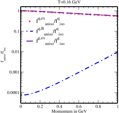
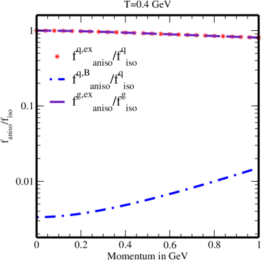
a	b

Figure 1: Variation of the ratio $f_{\rm aniso}/f_{\rm iso}$ with momentum in the presence of momentum anisotropies both due to asymptotic expansion and strong magnetic field ($15$ $m_{\pi}^{2}$) at (a) low temperature and (b) high temperature with the quasiparticle masses for quarks and gluons.

Before discussing the results on the shear viscosity and bulk viscosity in the presence of magnetic field-induced and expansion-induced anisotropies, it is utmost important to understand the behaviors of the isotropic and anisotropic distribution functions, because the behaviors of transport coefficients mainly depend on the phase-space factor, relaxation-time and the distribution function which in general embraces all the information on the influence of anisotropy. Thus, it becomes essential to explore the effects of anisotropies on quark and gluon distribution functions through their ratios with respect to their isotropic counterparts, viz. $f^{\rm q,\rm ex}_{\rm aniso}/f^{\rm q}_{\rm iso}$, $f^{\rm q,\rm B}_{\rm aniso}/f^{\rm q}_{\rm iso}$, $f^{\rm g,\rm ex}_{\rm aniso}/f^{\rm g}_{\rm iso}$ in figure 1 at two temperatures. We have employed the quasiparticle description in the distribution functions for the isotropic and expansion-driven anisotropic mediums by the $T$-dependent masses for gluons (1) and quarks (2), whereas the $T$ and $B$-dependent mass (18) has been used in the distribution function for the $B$-driven anisotropic medium. It is found that the effects of anisotropy caused by the expansion on quark and gluon distributions are almost identical (seen in figure 1), at least for the weak-anisotropic limit. However, the ratios get decreased in the high momentum regime. In the presence of strong magnetic field the distribution function for quark gets affected severely and the ratio in low momenta is tiny and increases at higher momenta. With the aforesaid findings on the distribution functions in the presence of anisotropies, we have computed the shear viscosity in isotropic (38), expansion- (52) and $B$-driven anisotropic (82) mediums and the bulk viscosity in isotropic (44), expansion- (54) and $B$-driven anisotropic (88) mediums. From figure 2a we have observed that, at low temperatures, the difference between the values of $\eta$ in isotropic medium and in the presence of weak-momentum anisotropy ($\xi=0.6$) due to asymptotic expansion is almost negligible, however, with the increase of temperature, this difference gradually increases, i.e. $\eta$ becomes smaller than its isotropic counterpart. If the origin of weak-momentum anisotropy is strong magnetic field, then the magnitude of $\eta$ becomes higher than that in isotropic medium and with temperature, this difference increases. Thus the above anisotropies leave different imprints on the shear viscosity, which are attributed mainly by the modified distribution function, phase space factor and relaxation-time in the absence and presence of strong magnetic field. Similarly, $\zeta$ gets amplified in $B$-driven anisotropy compared to both isotropic and expansion-driven anisotropic cases (in figure 2b). However with the increase of temperature, $\zeta$ decreases very slowly, opposite to a slow increase in isotropic medium. Interestingly, if the anisotropy is originated from the initial asymptotic expansion, then $\zeta$ becomes meagre and approaches zero at a higher temperature.

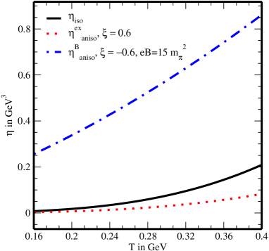
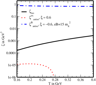
a	b

Figure 2: Variations of (a) the shear viscosity and (b) the bulk viscosity with temperature in the presence of momentum anisotropies both due to asymptotic expansion and strong magnetic field.

3.3 Ratios of the shear ($\eta/s$) and bulk ($\zeta/s$) viscosities to the entropy density

We are now going to study the effects of momentum anisotropies generated at the early stages of collisions in URHICs on the dimensionless ratios, $\eta/s$ and $\zeta/s$, because they are useful in characterizing how close the matter produced at URHICs is to being perfect and conformal fluid, respectively. The phenomenological studies by parton transport of the collective behavior [45, 46, 47, 48] have reported that the QGP has a very small value of $\eta/s\approx\frac{1}{4\pi}$, suggesting that the matter produced at RHIC is a strongly-coupled fluid of quarks and gluons, contrary to the belief of weakly interacting gas of quarks and gluons on the basis of asymptotic freedom. Similarly, the study of AdS/CFT correspondence [2] constrains the value of $\eta/s$ by a lower bound of $\frac{1}{4\pi}$. The hydrodynamic model [49] also with small value of $\eta/s$ ranging from $\frac{1}{4\pi}$ to $\frac{2}{4\pi}$ consistently reproduces the experimental data [50, 51] and lattice calculations [52, 53]. The bulk viscosity is yet to be developed at the early times of the hydrodynamic evolution, so some early viscous hydrodynamic simulations have usually ignored it in the dissipative part of energy-momentum tensor for simplicity [96, 97]. Although $\zeta$ vanishes for a thermal QCD medium of massless flavors on the classical level due to the conformal symmetry, but the nonabelian interactions break the conformal symmetry of QCD and generate a nonzero bulk viscosity, which is found in the lattice calculation of SU(3) gauge theory [54]. Near the critical or crossover temperature of hadron to QGP phase transition, the value of $\zeta/s$ becomes a maximum whereas that of $\eta/s$ becomes a minimum. Thus, it becomes worthwhile to observe the behaviors of both $\eta/s$ and $\zeta/s$ in the presence of $B$- and expansion-induced anisotropies, which in turn gives the effect of strong magnetic field through the anisotropy it generated. In order to do this, one thus requires the expression of the entropy density ($s$) in the presence of anisotropies, which could be best derived in the abovementioned kinetic theory approach. For the chemical potential of quarks, $\mu_{q}=0$, the entropy density is obtained from the energy density and pressure by the relation,

$$S=\frac{\varepsilon+P}{T}~{}.$$ (89)

Therefore we have first calculated the energy density and pressure in isotropic as well as in anisotropic mediums in appendix C, using the kinetic theory. Hence the above relation (89) has been used to obtain the entropy densities for isotropic, expansion-driven anisotropic and $B$-driven anisotropic mediums as

$$S^{\rm iso} = \frac{\beta}{3\pi^{2}}\sum_{i}g_{i}\int d{\rm p}~{}{\rm p}^{2}\left(\frac{{\rm p}^{2}}{\omega_{i}}+3\omega_{i}\right)f_{i}^{\rm iso}+\frac{\beta}{6\pi^{2}}g_{g}\int d{\rm p}~{}{\rm p}^{2}\left(\frac{{\rm p}^{2}}{\omega_{g}}+3\omega_{g}\right)f_{g}^{\rm iso},$$ (90)

$$S_{\rm ex}^{\rm aniso} = S^{\rm iso}-\frac{\xi\beta^{2}}{18\pi^{2}}\sum_{i}g_{i}\int d{\rm p}~{}\frac{{\rm p}^{4}}{\omega_{i}}\left(\frac{{\rm p}^{2}}{\omega_{i}}+3\omega_{i}\right)f_{i}^{\rm iso}(1-f_{i}^{\rm iso})$$ (91)

$$-\frac{\xi\beta^{2}}{36\pi^{2}}g_{g}\int d{\rm p}~{}\frac{{\rm p}^{4}}{\omega_{g}}\left(\frac{{\rm p}^{2}}{\omega_{g}}+3\omega_{g}\right)f_{g}^{\rm iso}(1+f_{g}^{\rm iso})$$

$$= S^{\rm iso}-\xi\left[\frac{\beta^{2}}{18\pi^{2}}\sum_{i}g_{i}\int d{\rm p}~{}\frac{{\rm p}^{4}}{\omega_{i}}\left(\frac{{\rm p}^{2}}{\omega_{i}}+3\omega_{i}\right)f_{i}^{\rm iso}(1-f_{i}^{\rm iso})\right.$$

$$\left.+\frac{\beta^{2}}{36\pi^{2}}g_{g}\int d{\rm p}~{}\frac{{\rm p}^{4}}{\omega_{g}}\left(\frac{{\rm p}^{2}}{\omega_{g}}+3\omega_{g}\right)f_{g}^{\rm iso}(1+f_{g}^{\rm iso})\right],$$

$$S_{\rm B}^{\rm aniso} = \frac{\beta}{2\pi^{2}}\sum_{i}g_{i}|q_{i}B|\int dp_{3}\left(\frac{p_{3}^{2}}{\omega_{i}}+\omega_{i}\right)f_{i}^{\xi=0}$$ (92)

$$-\frac{\xi\beta^{2}}{4\pi^{2}}\sum_{i}g_{i}|q_{i}B|\int dp_{3}~{}\frac{p_{3}^{2}}{\omega_{i}}\left(\frac{p_{3}^{2}}{\omega_{i}}+\omega_{i}\right)f_{i}^{\xi=0}(1-f_{i}^{\xi=0})$$

$$+\frac{\beta}{6\pi^{2}}g_{g}\int d{\rm p}~{}{\rm p}^{2}\left(\frac{{\rm p}^{2}}{\omega_{g}}+3\omega_{g}\right)f_{g}^{\rm iso}$$

$$= S^{\xi=0}-\frac{\xi\beta^{2}}{4\pi^{2}}\sum_{i}g_{i}|q_{i}B|\int dp_{3}~{}\frac{p_{3}^{2}}{\omega_{i}}\left(\frac{p_{3}^{2}}{\omega_{i}}+\omega_{i}\right)f_{i}^{\xi=0}(1-f_{i}^{\xi=0}),$$

respectively. The immediate observation is that the entropy density gets decreased in the presence of momentum anisotropy (seen in figure 3), especially it is lowest in $B$-driven anisotropy due to the severe reduction of phase-space in the presence of strong magnetic field.

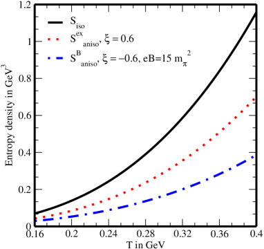
Figure 3: Variation of the entropy density with temperature in the presence of momentum anisotropies both due to asymptotic expansion and strong magnetic field.

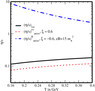
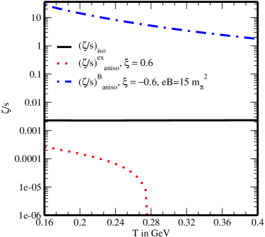
a	b

Figure 4: Variations of (a) ${\eta}/{s}$ and (b) ${\zeta}/{s}$ with temperature in the presence of momentum anisotropies both due to asymptotic expansion and strong magnetic field.

Thus, having the knowledge of entropy density in the presence of anisotropies, we have visualized the effects of anisotropies on the variations of $\eta/s$ and $\zeta/s$ with temperature in figures 4a and 4b, respectively. Since $s$ is always smaller than $\eta$ in $B$-driven anisotropy, $\eta/s$ is always larger than one, but unlike $\eta$ (as well as $s$), $\eta/s$ decreases with temperature (dashed-dotted line in figure 4a) because entropy density increases faster with $T$ than $\eta$. On the other hand, $\eta/s$ becomes much smaller ($<1$) in isotropic medium as well as in expansion-driven anisotropic medium (denoted by solid and dotted lines, respectively in figure 4a) than that in $B$-driven anisotropy, but $\eta/s$ increases with temperature monotonically, resulting finally the inequality: $\frac{\eta}{s}\big{|}_{\rm B-driven~{}aniso}>\frac{\eta}{s}\big{|}_{\rm iso}>\frac{\eta}{s}\big{|}_{\rm ex-driven~{}aniso}$. Shear viscosity in the isotropic case is known as collisional viscosity and the same arising due to weak-momentum anisotropy is called anomalous viscosity. In the theory of particle transport in turbulent plasma [98], it has been argued that, due to anomalous viscosity, even a weakly-coupled but expanding quark-gluon plasma may gain the character of a nearly perfect fluid, thus a large anisotropy describes a small value of anomalous viscosity. In our finding, the collisional viscosity comes out higher than the anomalous viscosity in expansion-driven anisotropy, thus the ratio $\eta/s$ indicates the character of nearly perfect fluid. On the other hand, the collisional viscosity is smaller than the anomalous viscosity in $B$-driven anisotropy, so $\eta/s$ takes the medium slightly away from the fluid character. Last but not the least, $\zeta/s$ is very small compared to $\eta/s$ except that in $B$-driven anisotropy, where it becomes comparable to $\eta/s$ and decreases with temperature (in figure 4b). However, like the variation of $\zeta$ with temperature, $\zeta/s$ in expansion-driven anisotropy vanishes at some higher temperature, which could have a resemblance with the temperature where the chiral symmetry is restored.

4 The coefficients affiliated to momentum, heat and charge transports

In this section, we are going to study the effects of anisotropies on the relative behaviors among momentum, heat and charge transports through the Prandtl number, the Reynolds number and the ratio between momentum diffusion and charge diffusion. To be specific, the $B$-driven anisotropy in a way reveals the effect of strong magnetic field on the abovementioned transport coefficients.

4.1 Prandtl number

The heat transfer and the momentum transfer in a medium are diffusive processes. The relative behavior between the momentum diffusion and the thermal diffusion can be described in terms of the Prandtl number,

$${\rm Pl}=\frac{\eta/\rho}{\kappa/C_{p}}~{},$$ (93)

where $C_{p}$ is the specific heat at constant pressure, $\rho$ denotes the mass density and $\kappa$ represents the thermal conductivity. Thus, Pl describes the roles of thermal conductivity and shear viscosity on the sound attenuation in the system and has been calculated in a varieties of systems, such as, strongly coupled liquid helium [56], nonrelativistic conformal holographic fluid [56, 57] and a dilute atomic Fermi gas [58] etc. The Prandtl number sheds light on the sound attenuation in the system, which in turn tells about the energy loss while sound propagates in a medium. The Prandtl number of magnitude less than one implies the dominance of thermal diffusion over momentum diffusion in the sound attenuation, whereas the opposite happens for Pl greater than one. In this work, we wish to find out how the presence of momentum anisotropies in a medium could affect the competition between momentum and heat diffusions, resulting in the energy dissipation of sound propagation. In this way the effect of magnetic field on the sound attenuation could be explored.

While calculating the Prandtl number, the expressions for the thermal conductivity and the specific heat at constant pressure in the similar environment are necessary. We have recently studied $\kappa$ [8], so we closely follow our results in appendix D. Next we have obtained $C_{p}$ from the following thermodynamic relation,

$$C_{p}=\frac{\partial(\varepsilon+P)}{\partial T}~{},$$ (94)

which has been calculated from the energy density and pressure in the similar environment. Thus we get the expressions of $C_{p}$ for isotropic, expansion-driven anisotropic and $B$-driven anisotropic mediums as

$$C_{p}^{\rm iso} = \frac{\beta^{2}}{3\pi^{2}}\sum_{i}g_{i}\int d{\rm p}~{}{\rm p}^{2}\left({\rm p}^{2}+3\omega_{i}^{2}\right)f_{i}^{\rm iso}(1-f_{i}^{\rm iso})$$ (95)

$$+\frac{\beta^{2}}{6\pi^{2}}g_{g}\int d{\rm p}~{}{\rm p}^{2}\left({\rm p}^{2}+3\omega_{g}^{2}\right)f_{g}^{\rm iso}(1+f_{g}^{\rm iso}),$$

$$C_{p,\rm ex}^{\rm aniso} = C_{p}^{\rm iso}+\frac{\xi\beta^{2}}{18\pi^{2}}\sum_{i}g_{i}\int d{\rm p}~{}\frac{{\rm p}^{4}}{\omega_{i}^{2}}\left({\rm p}^{2}+3\omega_{i}^{2}\right)f_{i}^{\rm iso}(1-f_{i}^{\rm iso})$$ (96)

$$-\frac{\xi\beta^{3}}{18\pi^{2}}\sum_{i}g_{i}\int d{\rm p}~{}\frac{{\rm p}^{4}}{\omega_{i}}\left({\rm p}^{2}+3\omega_{i}^{2}\right)f_{i}^{\rm iso}(1-f_{i}^{\rm iso})(1-2f_{i}^{\rm iso})$$

$$+\frac{\xi\beta^{2}}{36\pi^{2}}g_{g}\int d{\rm p}~{}\frac{{\rm p}^{4}}{\omega_{g}^{2}}\left({\rm p}^{2}+3\omega_{g}^{2}\right)f_{g}^{\rm iso}(1+f_{g}^{\rm iso})$$

$$-\frac{\xi\beta^{3}}{36\pi^{2}}g_{g}\int d{\rm p}~{}\frac{{\rm p}^{4}}{\omega_{g}}\left({\rm p}^{2}+3\omega_{g}^{2}\right)f_{g}^{\rm iso}(1+f_{g}^{\rm iso})(1+2f_{g}^{\rm iso})$$

$$= C_{p}^{\rm iso}+\xi\left[\frac{\beta^{3}}{18\pi^{2}}\sum_{i}g_{i}\int d{\rm p}~{}\frac{{\rm p}^{4}}{\omega_{i}}\left({\rm p}^{2}+3\omega_{i}^{2}\right)f_{i}^{\rm iso}(1-f_{i}^{\rm iso})\left\{\frac{1}{\beta\omega_{i}}-1+2f_{i}^{\rm iso}\right\}\right.$$

$$\left.+\frac{\beta^{3}}{36\pi^{2}}g_{g}\int d{\rm p}~{}\frac{{\rm p}^{4}}{\omega_{g}}\left({\rm p}^{2}+3\omega_{g}^{2}\right)f_{g}^{\rm iso}(1+f_{g}^{\rm iso})\left\{\frac{1}{\beta\omega_{g}}-1-2f_{g}^{\rm iso}\right\}\right],$$

$$C_{p,\rm B}^{\rm aniso} = \frac{\beta^{2}}{2\pi^{2}}\sum_{i}g_{i}|q_{i}B|\int dp_{3}\left(p_{3}^{2}+\omega_{i}^{2}\right)f_{i}^{\xi=0}(1-f_{i}^{\xi=0})$$ (97)

$$+\frac{\xi\beta^{2}}{4\pi^{2}}\sum_{i}g_{i}|q_{i}B|\int dp_{3}~{}\frac{p_{3}^{2}}{\omega_{i}^{2}}\left(p_{3}^{2}+\omega_{i}^{2}\right)f_{i}^{\xi=0}(1-f_{i}^{\xi=0})$$

$$-\frac{\xi\beta^{3}}{4\pi^{2}}\sum_{i}g_{i}|q_{i}B|\int dp_{3}~{}\frac{p_{3}^{2}}{\omega_{i}}\left(p_{3}^{2}+\omega_{i}^{2}\right)f_{i}^{\xi=0}(1-f_{i}^{\xi=0})(1-2f_{i}^{\xi=0})$$

$$+\frac{\beta^{2}}{6\pi^{2}}g_{g}\int d{\rm p}~{}{\rm p}^{2}\left({\rm p}^{2}+3\omega_{g}^{2}\right)f_{g}^{\rm iso}(1+f_{g}^{\rm iso})$$

$$= C_{p}^{\xi=0}+\xi\left[\frac{\beta^{3}}{4\pi^{2}}\sum_{i}g_{i}|q_{i}B|\int dp_{3}~{}\frac{p_{3}^{2}}{\omega_{i}}\left(p_{3}^{2}+\omega_{i}^{2}\right)f_{i}^{\xi=0}(1-f_{i}^{\xi=0})\right.$$

$$\left.\hskip 207.7052pt\times\left\{\frac{1}{\beta\omega_{i}}-1+2f_{i}^{\xi=0}\right\}\right],$$

respectively.

Finally the mass density ($\rho$) has been obtained from the product of the number densities of quarks and gluons with the respective quasiparticle masses as

$$\rho=2\sum_{i}m_{i}n_{i}+m_{g}n_{g}~{}.$$ (98)

The factor “2” represents the equal contributions from quark and antiquark due to $\mu_{q}=0$. Therefore, we get the expressions of $\rho$ for isotropic, expansion-driven anisotropic and $B$-driven anisotropic mediums as

$$\rho^{\rm iso} = \frac{1}{\pi^{2}}\sum_{i}m_{i}g_{i}\int d{\rm p}~{}{\rm p}^{2}f_{i}^{\rm iso}+\frac{1}{2\pi^{2}}m_{g}g_{g}\int d{\rm p}~{}{\rm p}^{2}f_{g}^{\rm iso},$$ (99)

$$\rho_{\rm ex}^{\rm aniso} = \rho^{\rm iso}-\frac{\xi\beta}{6\pi^{2}}\sum_{i}m_{i}g_{i}\int d{\rm p}~{}\frac{{\rm p}^{4}}{\omega_{i}}f_{i}^{\rm iso}(1-f_{i}^{\rm iso})-\frac{\xi\beta}{12\pi^{2}}m_{g}g_{g}\int d{\rm p}~{}\frac{{\rm p}^{4}}{\omega_{g}}f_{g}^{\rm iso}(1+f_{g}^{\rm iso})$$ (100)

$$= \rho^{\rm iso}-\xi\left[\frac{\beta}{6\pi^{2}}\sum_{i}m_{i}g_{i}\int d{\rm p}~{}\frac{{\rm p}^{4}}{\omega_{i}}f_{i}^{\rm iso}(1-f_{i}^{\rm iso})\right.$$

$$\left.+\frac{\beta}{12\pi^{2}}m_{g}g_{g}\int d{\rm p}~{}\frac{{\rm p}^{4}}{\omega_{g}}f_{g}^{\rm iso}(1+f_{g}^{\rm iso})\right],$$

$$\rho_{\rm B}^{\rm aniso} = \frac{1}{2\pi^{2}}\sum_{i}m_{i}g_{i}|q_{i}B|\int dp_{3}f_{i}^{\xi=0}-\frac{\xi\beta}{4\pi^{2}}\sum_{i}m_{i}g_{i}|q_{i}B|\int dp_{3}~{}\frac{p_{3}^{2}}{\omega_{i}}f_{i}^{\xi=0}(1-f_{i}^{\xi=0})$$ (101)

$$+\frac{1}{2\pi^{2}}m_{g}g_{g}\int d{\rm p}~{}{\rm p}^{2}f_{g}^{\rm iso}$$

$$= \rho^{\xi=0}-\frac{\xi\beta}{4\pi^{2}}\sum_{i}m_{i}g_{i}|q_{i}B|\int dp_{3}~{}\frac{p_{3}^{2}}{\omega_{i}}f_{i}^{\xi=0}(1-f_{i}^{\xi=0}),$$

respectively. We have therefore computed the Prandtl number as a function of temperature (seen in figure 5) and this is found to increase very slowly with the temperature. It maintains higher magnitude in $B$-driven anisotropy than in isotropic medium and expansion-driven anisotropic medium as well. In all cases Prandtl number remains greater than 1, implying that the sound attenuation is mostly governed by the momentum diffusion.

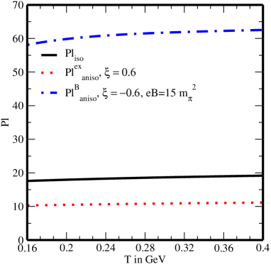
Figure 5: Variation of the Prandtl number with temperature in the presence of momentum anisotropies both due to asymptotic expansion and strong magnetic field.

4.2 Reynolds number

The Reynolds number plays a fundamental role in determining the magnitude of the kinematic viscosity (${\eta}/{\rho}$) as compared to the length and velocity of the flow of a liquid and is defined by

$${\rm Rl}=\frac{Lv}{\eta/\rho}~{},$$ (102)

where $L$ and $v$ are the characteristic length and velocity of the flow, respectively. From hydrodynamic point of view, the Reynolds number describes the motion of the fluid and when the nature of the flow gets converted from laminar into turbulent. This conversion happens when ${\rm Rl}$ is much larger than 1 or kinematic viscosity is very small in comparison to the product of characteristic length and velocity ($Lv$) [59]. In (3+1)-dimensional fluid dynamical model with globally symmetric, peripheral initial conditions, the value of the Rl is estimated in the range 3-10 for initial QGP with minimal viscosity to entropy density ratio, i.e., for $\eta/s=0.1$ [60], whereas the holographic model reports its upper bound as approximately 20 [59]. In this work, we have estimated the Reynolds number for (isotropic) thermal medium of quarks and gluons in kinetic theory approach in figure 6, which ranges 5.5 - 7 in the temperature range, 160 - 400 MeV (denoted by solid line). In addition, we have also estimated Rl for the same but it now exhibits momentum anisotropies, where the expansion-driven anisotropy enhances the number and the $B$-driven anisotropy does the opposite and that too makes it less than one (labelled as dotted and dashed-dotted lines, respectively), compared to the isotropic case.

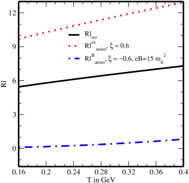
Figure 6: Variation of the Reynolds number with temperature in the presence of momentum anisotropies both due to asymptotic expansion and strong magnetic field for $L=3$ fm.

4.3 Relative behavior between momentum diffusion and charge diffusion

To understand the dominance of the momentum diffusion over the charge diffusion, one needs to estimate the ratio of the two dimensionless ratios: the first one is $\eta/s$ and the second one is $\sigma_{\rm el}/T$, representing the momentum and charge diffusions, respectively. Thus, the ratio is given by

$$\mathcal{\gamma}=\frac{\eta/s}{\sigma_{el}/T}~{},$$ (103)

where $\sigma_{\rm el}$ is the electrical conductivity. Unlike gluons, only quarks carry electric charge, hence they only contribute to the charge transport and thus contribute to the electrical conductivity. On the other hand, both quarks and gluons participate in the momentum transport, thus contribute to the shear viscosity. Therefore, for a QGP medium, $\sigma_{\rm el}/T$ is always smaller than $\eta/s$, resulting the ratio, $\gamma$ larger than 1. This understanding is evidenced in ref. [99], where it is found that the large scattering rates due to abundance of gluons in high temperature QGP (compared to quarks) can damp the electrical conductivity and it results in the enhancement of the ratio, $\gamma$. We now wish to compute $\gamma$ for the hot QCD matter in the presence of anisotropies and also to observe the effect of strong magnetic field, using the kinetic theory approach. Therefore, we need to have the ratio, $\sigma_{\rm el}/T$ in the identical environment, which has been recently calculated by us [8]. So, we closely follow our earlier calculation in appendix E.

In figure 7, we have plotted $\gamma$ (i.e., $(\eta/s)/(\sigma_{el}/T)$) as a function of temperature for isotropic medium as well as for expansion-driven and $B$-driven anisotropic mediums. The ratio $\eta/s$ is influenced by both gluon-gluon and quark-quark scatterings, while $\sigma_{el}/T$ is influenced only by the quark-quark scattering as only charged particles contribute to the electrical conductivity. Thus, the variation of $\gamma$ with temperature can explain the contest between gluon and quark contributions to the total scattering cross section. We have found that for an isotropic medium, $\gamma$ (denoted by the solid line) is maximum around $T_{c}$ ($T_{c}=0.16$ GeV) and decreases very slowly with temperature. This is due to the fact that although the magnitude of $\eta/s$ is higher than $\sigma_{\rm el}/T$ but the latter increases relatively faster than the former. In the presence of expansion-driven anisotropy (denoted by dotted line), $\gamma$ becomes smaller than the isotropic case which is due to the relative decrease of $\eta/s$ than $\sigma_{\rm el}/T$ caused by the anisotropy. On the contrary, in the presence of strong magnetic field, the ratio becomes much larger than the isotropic case, which could be understood as follows: Although the gluon phase-space remains unaltered, but the quark phase-space gets reduced severely in a strong magnetic field, resulting an overall decrease in total entropy density. Hence $\eta/s$ gets enhanced by two orders of magnitude. On the other hand, the large increase of collisional relaxation time in strong magnetic field compensates the reduction in quark phase-space, resulting an increase in $\sigma_{\rm el}/T$ ratio, but it is now increased by one order of magnitude. Therefore the ratio, $\gamma$ gets increased by one order of magnitude. In brief, $\gamma$ remains larger than unity, so the momentum diffusion prevails over the charge diffusion.

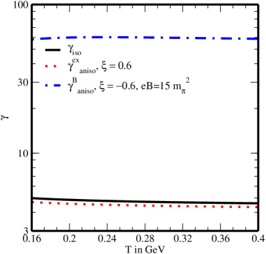
Figure 7: Variation of $\gamma=(\eta/s)/(\sigma_{el}/T)$ with temperature in the presence of momentum anisotropies both due to asymptotic expansion and strong magnetic field.

5 Conclusions

In the present work, we have first studied the momentum transports through the shear and bulk viscosities of a hot QCD matter and then the interplays among momentum, charge and heat transports are delved by the Prandtl number, the Reynold number and the relative behavior between momentum diffusion and charge diffusion. Most importantly, the abovementioned studies have been extended to the medium with weak momentum anisotropies, which in turn explore the effects of strong magnetic field and asymptotic expansion which thought to be present at the initial stages of ultrarelativistic heavy ion collisions. We have calculated the aforesaid coefficients in the kinetic theory approach via the relativistic Boltzmann transport equation in the relaxation-time approximation and the interactions among partons are subsumed through the quasiparticle masses at finite temperature and strong magnetic field.

For that purpose, we have started with computing the shear and bulk viscosities in the absence and presence of expansion- and $B$-driven anisotropies of a thermal QCD medium. Overall observation is that the presence of anisotropy due to strong magnetic field enhances both $\eta$ and $\zeta$ substantially, facilitating the transports of momentum across and along the layer, compared to either isotropic scenario or expansion-driven anisotropic scenario. Moreover, the aforesaid anisotropies affect $\eta$ and $\zeta$ differently with respect to the isotropic medium as a reference, therefore the viscosities can in principle distinguish the abovementioned anisotropies. Next we have computed the $\eta/s$ and $\zeta/s$ ratios to see how the fluidity and the location of the transition point (related to the chiral symmetry) get affected by the anisotropies, respectively. This enriches a competition between the enhancement of momentum transport and the reduction of phase-space (entropy density) in the presence of $B$-induced anisotropy, resulting the ratios, $\eta/s$ and $\zeta/s$ much greater than one, but unlike $\eta$ and $\zeta$, the ratios now decrease with the temperature. On the other hand, in the presence of expansion-driven anisotropy, both ratios become much smaller and specifically $\zeta/s$ vanishes around $T=0.28$ GeV.

In the next part, we have looked into the interplay of transports between momentum and heat by the Prandtl number (Pl), between momentum and size of the medium by the Reynolds number (Rl) and between momentum and charge by the ratio, $\gamma$ in the presence of anisotropies. The presence of strong magnetic field makes Pl much larger than its values in the absence of magnetic field (isotropic) as well as expansion-driven anisotropy. Thus, in the strong magnetic field regime, the sound attenuation is mostly governed by the momentum diffusion. However, the magnetic field drops the Reynolds number to the value less than unity, i.e., the kinematic viscosity dominates over the characteristic length and velocity of the system, which is just opposite to the effect caused by the expansion-driven anisotropy. Our final observation is that the dominance of momentum diffusion over charge diffusion is more pronounced in strong magnetic field than in other scenarios. However, the former one always prevails over the latter one.

6 Acknowledgment

One of us (B. K. P.) is thankful to Council of Scientific and Industrial Research (Grant No. 03(1407)/17/EMR-II) for the financial support of this work.

Appendix A Thermal quark mass at finite magnetic field

To compute the self-energy (6) at finite temperature, we have obtained the forms of quark and gluon propagators at finite temperature in the imaginary time formalism, where the continuous energy integral ($\int\frac{dp_{0}}{2\pi}$) is replaced by the discrete Matsubara frequency sum. Due the presence of strong magnetic field (along $z$-direction), the transverse component of momentum $k_{\perp}\approx 0$, so, $e^{-k^{2}_{\perp}/|q_{i}B|}$ in eq. (9) becomes unity and the integration over the transverse component of the momentum gives the factor $|q_{i}B|$. So the quark self-energy (6) in the SMF limit takes the following form,

$$\Sigma(p_{\parallel}) = \frac{2g^{2}}{3\pi^{2}}|q_{i}B|T\sum_{n}\int dk_{z}\frac{\left[\left(1+\gamma^{0}\gamma^{3}\gamma^{5}\right)\left(\gamma^{0}k_{0}-\gamma^{3}k_{z}\right)-2m_{i}\right]}{\left[k_{0}^{2}-\omega^{2}_{k}\right]\left[(p_{0}-k_{0})^{2}-\omega_{pk}^{2}\right]}$$ (A.104)

$$= \frac{2g^{2}|q_{i}B|}{3\pi^{2}}\int dk_{z}\left[(\gamma^{0}+\gamma^{3}\gamma^{5})L^{1}-(\gamma^{3}+\gamma^{0}\gamma^{5})k_{z}L^{2}\right],$$

where $\omega^{2}_{k}=k_{z}^{2}+m_{i}^{2}$, $\omega_{pk}^{2}=(p_{z}-k_{z})^{2}$, and $L^{1}$ and $L^{2}$ represent two frequency sums, whose forms are given by

$$L^{1}=T\sum_{n}~{}\frac{k_{0}}{\left[k_{0}^{2}-\omega_{k}^{2}\right]\left[(p_{0}-k_{0})^{2}-\omega_{pk}^{2}\right]}~{},$$ (A.105)

$$L^{2}=T\sum_{n}\frac{1}{\left[k_{0}^{2}-\omega_{k}^{2}\right]\left[(p_{0}-k_{0})^{2}-\omega_{pk}^{2}\right]}~{}.$$ (A.106)

After using the values of the above frequency sums, the form of the self-energy (A.104) turns out to be

$$\Sigma(p_{\parallel})=\frac{g^{2}|q_{i}B|}{3\pi^{2}}\int\frac{dk_{z}}{\omega_{k}}\left[\frac{1}{e^{\beta\omega_{k}}-1}+\frac{1}{e^{\beta\omega_{k}}+1}\right]\left[\frac{\gamma^{0}p_{0}+\gamma^{3}p_{z}}{p_{\parallel}^{2}}+\frac{\gamma^{0}\gamma^{5}p_{z}+\gamma^{3}\gamma^{5}p_{0}}{p_{\parallel}^{2}}\right],$$ (A.107)

which after the integration over $k_{z}$, becomes

$$\Sigma(p_{\parallel})=\frac{g^{2}|q_{i}B|}{3\pi^{2}}\left[\frac{\pi T}{2m_{i}}-\ln(2)\right]\left[\frac{\gamma^{0}p_{0}}{p_{\parallel}^{2}}+\frac{\gamma^{3}p_{z}}{p_{\parallel}^{2}}+\frac{\gamma^{0}\gamma^{5}p_{z}}{p_{\parallel}^{2}}+\frac{\gamma^{3}\gamma^{5}p_{0}}{p_{\parallel}^{2}}\right].$$ (A.108)

The covariant structure of the quark self-energy at finite temperature and finite magnetic field is written as

$$\Sigma(p_{\parallel})=A\gamma^{\mu}u_{\mu}+B\gamma^{\mu}b_{\mu}+C\gamma^{5}\gamma^{\mu}u_{\mu}+D\gamma^{5}\gamma^{\mu}b_{\mu}~{},$$ (A.109)

where $A$, $B$, $C$ and $D$ denote the form factors, and $u^{\mu}$ (1,0,0,0) and $b^{\mu}$ (0,0,0,-1) represent the preferred directions of the heat bath and the magnetic field, respectively. Due to the introduction of these vectors the Lorentz and rotational symmetries are broken. In LLL approximation, the form factors are obtained as

$$A=\frac{1}{4}{\rm Tr}\left[\Sigma\gamma^{\mu}u_{\mu}\right]=\frac{g^{2}|q_{i}B|}{3\pi^{2}}\left[\frac{\pi T}{2m_{i}}-\ln(2)\right]\frac{p_{0}}{p_{\parallel}^{2}}~{},$$ (A.110)

$$B=-\frac{1}{4}{\rm Tr}\left[\Sigma\gamma^{\mu}b_{\mu}\right]=\frac{g^{2}|q_{i}B|}{3\pi^{2}}\left[\frac{\pi T}{2m_{i}}-\ln(2)\right]\frac{p_{z}}{p_{\parallel}^{2}}~{},$$ (A.111)

$$C=\frac{1}{4}{\rm Tr}\left[\gamma^{5}\Sigma\gamma^{\mu}u_{\mu}\right]=-\frac{g^{2}|q_{i}B|}{3\pi^{2}}\left[\frac{\pi T}{2m_{i}}-\ln(2)\right]\frac{p_{z}}{p_{\parallel}^{2}}~{},$$ (A.112)

$$D=-\frac{1}{4}{\rm Tr}\left[\gamma^{5}\Sigma\gamma^{\mu}b_{\mu}\right]=-\frac{g^{2}|q_{i}B|}{3\pi^{2}}\left[\frac{\pi T}{2m_{i}}-\ln(2)\right]\frac{p_{0}}{p_{\parallel}^{2}}~{},$$ (A.113)

where we found that $C=-B$ and $D=-A$.

In terms of the right-handed ($P_{R}=(1+\gamma^{5})/2$) and left-handed ($P_{L}=(1-\gamma^{5})/2$) chiral projection operators, the quark self-energy (A.109) is written as

$$\Sigma(p_{\parallel})=P_{R}\left[(A+C)\gamma^{\mu}u_{\mu}+(B+D)\gamma^{\mu}b_{\mu}\right]P_{L}+P_{L}\left[(A-C)\gamma^{\mu}u_{\mu}+(B-D)\gamma^{\mu}b_{\mu}\right]P_{R}~{},$$ (A.114)

which for $C=-B$ and $D=-A$, turns out to be

$$\Sigma(p_{\parallel})=P_{R}\left[(A-B)\gamma^{\mu}u_{\mu}+(B-A)\gamma^{\mu}b_{\mu}\right]P_{L}+P_{L}\left[(A+B)\gamma^{\mu}u_{\mu}+(B+A)\gamma^{\mu}b_{\mu}\right]P_{R}~{}.$$ (A.115)

In the strong magnetic field regime, the effective quark propagator can be derived from the following self-consistent Schwinger-Dyson equation,

$$S^{-1}(p_{\parallel})=\gamma^{\mu}p_{\parallel\mu}-\Sigma(p_{\parallel})~{},$$ (A.116)

which, in terms of projection operators, is rewritten as

$$S^{-1}(p_{\parallel})=P_{R}\gamma^{\mu}X_{\mu}P_{L}+P_{L}\gamma^{\mu}Y_{\mu}P_{R}~{},$$ (A.117)

where

$$\gamma^{\mu}X_{\mu}=\gamma^{\mu}p_{\parallel\mu}-(A-B)\gamma^{\mu}u_{\mu}-(B-A)\gamma^{\mu}b_{\mu}~{},$$ (A.118)

$$\gamma^{\mu}Y_{\mu}=\gamma^{\mu}p_{\parallel\mu}-(A+B)\gamma^{\mu}u_{\mu}-(B+A)\gamma^{\mu}b_{\mu}~{}.$$ (A.119)

Now the effective propagator takes the following form,

$$S(p_{\parallel})=\frac{1}{2}\left[P_{R}\frac{\gamma^{\mu}Y_{\mu}}{Y^{2}/2}P_{L}+P_{L}\frac{\gamma^{\mu}X_{\mu}}{X^{2}/2}P_{R}\right],$$ (A.120)

where

$$\frac{X^{2}}{2}=X_{1}^{2}=\frac{1}{2}\left[p_{0}-(A-B)\right]^{2}-\frac{1}{2}\left[p_{z}+(B-A)\right]^{2}~{},$$ (A.121)

$$\frac{Y^{2}}{2}=Y_{1}^{2}=\frac{1}{2}\left[p_{0}-(A+B)\right]^{2}-\frac{1}{2}\left[p_{z}+(B+A)\right]^{2}~{}.$$ (A.122)

After taking $p_{0}=0,p_{z}\rightarrow 0$ limit of either $X_{1}^{2}$ or $Y_{1}^{2}$ (which are equal in this limit), we get the thermal mass (squared) at finite temperature and strong magnetic field as

$$m_{iT,B}^{2}=X_{1}^{2}\Big{|}_{p_{0}=0,p_{z}\rightarrow 0}=Y_{1}^{2}\Big{|}_{p_{0}=0,p_{z}\rightarrow 0}=\frac{g^{2}|q_{i}B|}{3\pi^{2}}\left[\frac{\pi T}{2m_{i}}-\ln(2)\right].$$ (A.123)

Appendix B Form of $\Delta\tilde{T}^{ij}$ in the presence of strong magnetic field

In the presence of strong magnetic field, $\tilde{T}^{\mu\nu}$ and $\tilde{n}^{\mu}$ are defined as

$$\tilde{T}^{\mu\nu} = (\epsilon+P){u}^{\mu}{u}^{\nu}-Pg_{\parallel}^{\mu\nu}+\Delta\tilde{T}^{\mu\nu}$$ (B.124)

$$= \omega{u}^{\mu}{u}^{\nu}-Pg_{\parallel}^{\mu\nu}+\Delta\tilde{T}^{\mu\nu},$$

$$\tilde{n}^{\mu} = n{u}^{\mu}+\tilde{\gamma}^{\mu},$$ (B.125)

where $\Delta\tilde{T}^{\mu\nu}$, $\omega$, $n$ and $\tilde{\gamma}^{\mu}$ are the viscous stress tensor, the enthalpy, the particle number density and the dissipative correction to $\tilde{n}^{\mu}$, respectively in the presence of strong magnetic field. In addition, $g_{\parallel}^{\mu\nu}$ is defined as $g_{\parallel}^{\mu\nu}=(1,0,0,-1)$. Equations of motion are written as

$$\frac{\partial\tilde{T}_{\mu}^{\nu}}{\partial\tilde{x}^{\nu}} = 0,$$ (B.126)

$$\frac{\partial\tilde{n}^{\mu}}{\partial\tilde{x}^{\mu}} = 0,$$ (B.127)

where $\tilde{x}^{\mu}=(x^{0},0,0,x^{3})$ is redefined for the calculation in strong magnetic field.

From equations (B.124) and (B.126), we obtain

$${u}_{\mu}\frac{\partial}{\partial\tilde{x}^{\nu}}\left(\omega{u}^{\nu}\right)+\omega{u}^{\nu}\frac{\partial\tilde{u_{\mu}}}{\partial\tilde{x}^{\nu}}-\frac{\partial}{\partial\tilde{x}^{\nu}}\left(Pg_{\parallel\mu}^{\nu}\right)+\frac{\partial\Delta\tilde{T}_{\mu}^{\nu}}{\partial\tilde{x}^{\nu}} = 0.$$ (B.128)

Now multiplying ${u}^{\mu}$ on both sides of the above equation and simplifying, we get

$$\frac{\partial}{\partial\tilde{x}^{\nu}}\left(\omega{u}^{\nu}\right)-{u}^{\nu}\frac{\partial P}{\partial\tilde{x}^{\nu}}+{u}^{\mu}\frac{\partial\Delta\tilde{T}_{\mu}^{\nu}}{\partial\tilde{x}^{\nu}} = 0.$$ (B.129)

From equations (B.125) and (B.127), we get

$$\frac{\partial}{\partial\tilde{x}^{\mu}}\left(n{u}^{\mu}\right) = -\frac{\partial\tilde{\gamma}^{\mu}}{\partial\tilde{x}^{\mu}}.$$ (B.130)

Equation (B.130) is known as the “equation of continuity”. Using the identity $\omega{u}^{\nu}=n{u}^{\nu}\frac{\omega}{n}$ in eq. (B.129), we have

$$\frac{\omega}{n}\frac{\partial}{\partial\tilde{x}^{\nu}}\left(n{u}^{\nu}\right)+n{u}^{\nu}\frac{\partial}{\partial\tilde{x}^{\nu}}\left(\frac{\omega}{n}\right)-{u}^{\nu}\frac{\partial P}{\partial\tilde{x}^{\nu}}+{u}^{\mu}\frac{\partial\Delta\tilde{T}_{\mu}^{\nu}}{\partial\tilde{x}^{\nu}} = 0,$$ (B.131)

which with the help of the equation of continuity (B.130) becomes

$$-\frac{\omega}{n}\frac{\partial\tilde{\gamma}^{\nu}}{\partial\tilde{x}^{\nu}}+n{u}^{\nu}\frac{\partial}{\partial\tilde{x}^{\nu}}\left(\frac{\omega}{n}\right)-{u}^{\nu}\frac{\partial P}{\partial\tilde{x}^{\nu}}+{u}^{\mu}\frac{\partial\Delta\tilde{T}_{\mu}^{\nu}}{\partial\tilde{x}^{\nu}} = 0.$$ (B.132)

With the thermodynamic relation : $d\left(\frac{\omega}{n}\right)=Td\left(\frac{s}{n}\right)+\frac{1}{n}dP$, we have $\frac{\partial}{\partial\tilde{x}^{\nu}}\left(\frac{\omega}{n}\right)=T\frac{\partial}{\partial\tilde{x}^{\nu}}\left(\frac{s}{n}\right)+\frac{1}{n}\frac{\partial P}{\partial\tilde{x}^{\nu}}$, where $s$ is the entropy per unit proper volume. Now, eq. (B.132) takes the following form,

$$-\frac{\omega}{n}\frac{\partial\tilde{\gamma}^{\nu}}{\partial\tilde{x}^{\nu}}+n{u}^{\nu}\left[T\frac{\partial}{\partial\tilde{x}^{\nu}}\left(\frac{s}{n}\right)+\frac{1}{n}\frac{\partial P}{\partial\tilde{x}^{\nu}}\right]-{u}^{\nu}\frac{\partial P}{\partial\tilde{x}^{\nu}}+{u}^{\mu}\frac{\partial\Delta\tilde{T}_{\mu}^{\nu}}{\partial\tilde{x}^{\nu}} = 0,$$ (B.133)

which after simplification becomes

$$-\frac{\omega}{n}\frac{\partial\tilde{\gamma}^{\nu}}{\partial\tilde{x}^{\nu}}+n{u}^{\nu}T\frac{\partial}{\partial\tilde{x}^{\nu}}\left(\frac{s}{n}\right)+{u}^{\mu}\frac{\partial\Delta\tilde{T}_{\mu}^{\nu}}{\partial\tilde{x}^{\nu}} = 0.$$ (B.134)

The second term in l.h.s. of the above eq. (B.134) can be written as

$$n{u}^{\nu}T\frac{\partial}{\partial\tilde{x}^{\nu}}\left(\frac{s}{n}\right) = T\frac{\partial}{\partial\tilde{x}^{\nu}}\left(\frac{s}{n}n{u}^{\nu}\right)-T\frac{s}{n}\frac{\partial}{\partial\tilde{x}^{\nu}}\left(n{u}^{\nu}\right)$$ (B.135)

$$= T\frac{\partial}{\partial\tilde{x}^{\nu}}\left(s{u}^{\nu}\right)+T\frac{s}{n}\frac{\partial\tilde{\gamma}^{\nu}}{\partial\tilde{x}^{\nu}}.$$

Using eq. (B.135) in eq. (B.134), we get

$$-\frac{\omega}{n}\frac{\partial\tilde{\gamma}^{\nu}}{\partial\tilde{x}^{\nu}}+T\frac{\partial}{\partial\tilde{x}^{\nu}}\left(s{u}^{\nu}\right)+T\frac{s}{n}\frac{\partial\tilde{\gamma}^{\nu}}{\partial\tilde{x}^{\nu}}+{u}^{\mu}\frac{\partial\Delta\tilde{T}_{\mu}^{\nu}}{\partial\tilde{x}^{\nu}} = 0.$$ (B.136)

After rearranging the terms, the above equation tuns out to be

$$\left(\frac{\omega-Ts}{n}\right)\frac{\partial\tilde{\gamma}^{\nu}}{\partial\tilde{x}^{\nu}}-T\frac{\partial}{\partial\tilde{x}^{\nu}}\left(s{u}^{\nu}\right)-{u}^{\mu}\frac{\partial\Delta\tilde{T}_{\mu}^{\nu}}{\partial\tilde{x}^{\nu}} = 0,$$ (B.137)

where $\frac{\omega-Ts}{n}=\mu=$relativistic chemical potential. So, in terms of $\mu$, eq. (B.137) is rewritten as

$$\frac{\partial}{\partial\tilde{x}^{\nu}}\left(s{u}^{\nu}\right)-\frac{\mu}{T}\frac{\partial\tilde{\gamma}^{\nu}}{\partial\tilde{x}^{\nu}}+\frac{{u}^{\mu}}{T}\frac{\partial\Delta\tilde{T}_{\mu}^{\nu}}{\partial\tilde{x}^{\nu}} = 0,$$ (B.138)

which can be further simplified into

$$\frac{\partial}{\partial\tilde{x}^{\nu}}\left(s{u}^{\nu}\right)-\frac{\partial}{\partial\tilde{x}^{\nu}}\left(\frac{\mu}{T}\tilde{\gamma}^{\nu}\right)+\tilde{\gamma}^{\nu}\frac{\partial}{\partial\tilde{x}^{\nu}}\left(\frac{\mu}{T}\right)+\frac{1}{T}\frac{\partial}{\partial\tilde{x}^{\nu}}\left({u}^{\mu}\Delta\tilde{T}_{\mu}^{\nu}\right)-\frac{\Delta\tilde{T}_{\mu}^{\nu}}{T}\frac{\partial{u}^{\mu}}{\partial\tilde{x}^{\nu}}=0.$$ (B.139)

Using ${u}^{\mu}\Delta\tilde{T}_{\mu}^{\nu}=0$ in the above eq. (B.139), we get

$$\frac{\partial}{\partial\tilde{x}^{\nu}}\left(s{u}^{\nu}\right)-\frac{\partial}{\partial\tilde{x}^{\nu}}\left(\frac{\mu}{T}\tilde{\gamma}^{\nu}\right)+\tilde{\gamma}^{\nu}\frac{\partial}{\partial\tilde{x}^{\nu}}\left(\frac{\mu}{T}\right)-\frac{\Delta\tilde{T}_{\mu}^{\nu}}{T}\frac{\partial{u}^{\mu}}{\partial\tilde{x}^{\nu}} = 0,$$ (B.140)

which after simplification becomes

$$\frac{\partial}{\partial\tilde{x}^{\nu}}\left(s{u}^{\nu}-\frac{\mu}{T}\tilde{\gamma}^{\nu}\right) = -\tilde{\gamma}^{\nu}\frac{\partial}{\partial\tilde{x}^{\nu}}\left(\frac{\mu}{T}\right)+\frac{\Delta\tilde{T}_{\mu}^{\nu}}{T}\frac{\partial{u}^{\mu}}{\partial\tilde{x}^{\nu}}.$$ (B.141)

In eq. (B.141), $s{u}^{\nu}-\frac{\mu}{T}\tilde{\gamma}^{\nu}=\tilde{s}^{\nu}=$entropy flux density 4-vector in the presence of strong magnetic field. So, in terms of $\tilde{s}^{\nu}$, eq. (B.141) is rewritten as

$$\frac{\partial\tilde{s}^{\nu}}{\partial\tilde{x}^{\nu}} = -\tilde{\gamma}^{\nu}\frac{\partial}{\partial\tilde{x}^{\nu}}\left(\frac{\mu}{T}\right)+\frac{\Delta\tilde{T}_{\mu}^{\nu}}{T}\frac{\partial{u}^{\mu}}{\partial\tilde{x}^{\nu}}.$$ (B.142)

Here $\frac{\partial\tilde{s}^{\nu}}{\partial\tilde{x}^{\nu}}$ is the 4-divergence of the entropy flux density in a strong magnetic field. According to the law of increase of entropy, the r.h.s. of eq. (B.142) must be positive. Thus, a most general form of $\Delta\tilde{T}^{\mu\nu}$ that satisfies $\Delta\tilde{T}^{\mu\nu}{u}_{\nu}=0$ and the law of increase of entropy is written as

$$\Delta\tilde{T}^{\mu\nu}=-\eta^{B}\left(\frac{\partial{u}^{\mu}}{\partial\tilde{x}_{\nu}}+\frac{\partial{u}^{\nu}}{\partial\tilde{x}_{\mu}}-{u}^{\nu}{u}_{\lambda}\frac{\partial{u}^{\mu}}{\partial\tilde{x}_{\lambda}}-{u}^{\mu}{u}_{\lambda}\frac{\partial{u}^{\nu}}{\partial\tilde{x}_{\lambda}}-\frac{2}{3}\Delta_{\parallel}^{\mu\nu}\frac{\partial{u}^{\lambda}}{\partial\tilde{x}^{\lambda}}\right)-\zeta^{B}\Delta_{\parallel}^{\mu\nu}\frac{\partial{u}^{\lambda}}{\partial\tilde{x}^{\lambda}},$$ (B.143)

where $\Delta_{\parallel}^{\mu\nu}=g_{\parallel}^{\mu\nu}-{u}^{\mu}{u}^{\nu}$, $\eta^{B}$ and $\zeta^{B}$ are the shear viscosity and the bulk viscosity, respectively in the presence of strong magnetic field. In the local rest frame, the spatial component of velocity is zero, but its spatial derivative remains finite. Therefore, the spatial component of eq. (B.143) is written as

$$\Delta\tilde{T}^{ij} = -\eta^{B}\left(\frac{\partial{u}^{i}}{\partial\tilde{x}_{j}}+\frac{\partial{u}^{j}}{\partial\tilde{x}_{i}}-\frac{2}{3}\delta^{ij}\frac{\partial{u}^{l}}{\partial\tilde{x}^{l}}\right)-\zeta^{B}\delta^{ij}\frac{\partial{u}^{l}}{\partial\tilde{x}^{l}}$$ (B.144)

$$= -\eta^{B}\left(\partial^{i}{u}^{j}+\partial^{j}{u}^{i}-\frac{2}{3}\delta^{ij}\partial_{l}{u}^{l}\right)-\zeta^{B}\delta^{ij}\partial_{l}{u}^{l}$$

$$= -\eta^{B}{W}^{ij}-\zeta^{B}\delta^{ij}\partial_{l}{u}^{l}.$$

Appendix C Energy density and pressure

The thermodynamic quantities, such as, the energy density ($\varepsilon$) and the pressure ($P$) can be obtained from the energy momentum tensor ($T^{\mu\nu}$). In the absence of magnetic field, we have

$$\varepsilon = u_{\mu}T^{\mu\nu}u_{\nu},$$ (C.145)

$$P = -\frac{1}{3}\left(g_{\mu\nu}-u_{\mu}u_{\nu}\right)T^{\mu\nu},$$ (C.146)

whereas in the presence of strong magnetic field, the definitions of the energy density and the pressure get modified as

$$\varepsilon = u_{\mu}\tilde{T}^{\mu\nu}u_{\nu},$$ (C.147)

$$P = -\left(g^{\parallel}_{\mu\nu}-u_{\mu}u_{\nu}\right)\tilde{T}^{\mu\nu}.$$ (C.148)

Expressions of energy density for isotropic, expansion-driven anisotropic and $B$-driven anisotropic mediums are calculated as

$$\varepsilon^{\rm iso} = \frac{1}{\pi^{2}}\sum_{i}g_{i}\int d{\rm p}~{}{\rm p}^{2}\omega_{i}f_{i}^{\rm iso}+\frac{1}{2\pi^{2}}g_{g}\int d{\rm p}~{}{\rm p}^{2}\omega_{g}f_{g}^{\rm iso},$$ (C.149)

$$\varepsilon_{\rm ex}^{\rm aniso} = \varepsilon^{\rm iso}-\frac{\xi\beta}{6\pi^{2}}\sum_{i}g_{i}\int d{\rm p}~{}{{\rm p}^{4}}f_{i}^{\rm iso}(1-f_{i}^{\rm iso})$$ (C.150)

$$-\frac{\xi\beta}{12\pi^{2}}g_{g}\int d{\rm p}~{}{{\rm p}^{4}}f_{g}^{\rm iso}(1+f_{g}^{\rm iso})$$

$$= \varepsilon^{\rm iso}-\xi\left[\frac{\beta}{6\pi^{2}}\sum_{i}g_{i}\int d{\rm p}~{}{{\rm p}^{4}}f_{i}^{\rm iso}(1-f_{i}^{\rm iso})\right.$$

$$\left.+\frac{\beta}{12\pi^{2}}g_{g}\int d{\rm p}~{}{{\rm p}^{4}}f_{g}^{\rm iso}(1+f_{g}^{\rm iso})\right],$$

$$\varepsilon_{\rm B}^{\rm aniso} = \frac{1}{2\pi^{2}}\sum_{i}g_{i}|q_{i}B|\int dp_{3}\omega_{i}f_{i}^{\xi=0}$$ (C.151)

$$-\frac{\xi\beta}{4\pi^{2}}\sum_{i}g_{i}|q_{i}B|\int dp_{3}~{}{p_{3}^{2}}f_{i}^{\xi=0}(1-f_{i}^{\xi=0})$$

$$+\frac{1}{2\pi^{2}}g_{g}\int d{\rm p}~{}{\rm p}^{2}\omega_{g}f_{g}^{\rm iso}$$

$$= \varepsilon^{\xi=0}-\frac{\xi\beta}{4\pi^{2}}\sum_{i}g_{i}|q_{i}B|\int dp_{3}~{}{p_{3}^{2}}f_{i}^{\xi=0}(1-f_{i}^{\xi=0}),$$

respectively.

Expressions of pressure for isotropic, expansion-driven anisotropic and $B$-driven anisotropic mediums are calculated as

$$P^{\rm iso} = \frac{1}{3\pi^{2}}\sum_{i}g_{i}\int d{\rm p}~{}\frac{{\rm p}^{4}}{\omega_{i}}f_{i}^{\rm iso}+\frac{1}{6\pi^{2}}g_{g}\int d{\rm p}~{}\frac{{\rm p}^{4}}{\omega_{g}}f_{g}^{\rm iso},$$ (C.152)

$$P_{\rm ex}^{\rm aniso} = P^{\rm iso}-\frac{\xi\beta}{18\pi^{2}}\sum_{i}g_{i}\int d{\rm p}~{}\frac{{\rm p}^{6}}{\omega_{i}^{2}}f_{i}^{\rm iso}(1-f_{i}^{\rm iso})$$ (C.153)

$$-\frac{\xi\beta}{36\pi^{2}}g_{g}\int d{\rm p}~{}\frac{{\rm p}^{6}}{\omega_{g}^{2}}f_{g}^{\rm iso}(1+f_{g}^{\rm iso})$$

$$= P^{\rm iso}-\xi\left[\frac{\beta}{18\pi^{2}}\sum_{i}g_{i}\int d{\rm p}~{}\frac{{\rm p}^{6}}{\omega_{i}^{2}}f_{i}^{\rm iso}(1-f_{i}^{\rm iso})\right.$$

$$\left.+\frac{\beta}{36\pi^{2}}g_{g}\int d{\rm p}~{}\frac{{\rm p}^{6}}{\omega_{g}^{2}}f_{g}^{\rm iso}(1+f_{g}^{\rm iso})\right],$$

$$P_{\rm B}^{\rm aniso} = \frac{1}{2\pi^{2}}\sum_{i}g_{i}|q_{i}B|\int dp_{3}\frac{p_{3}^{2}}{\omega_{i}}f_{i}^{\xi=0}$$ (C.154)

$$-\frac{\xi\beta}{4\pi^{2}}\sum_{i}g_{i}|q_{i}B|\int dp_{3}~{}\frac{p_{3}^{4}}{\omega_{i}^{2}}f_{i}^{\xi=0}(1-f_{i}^{\xi=0})$$

$$+\frac{1}{6\pi^{2}}g_{g}\int d{\rm p}~{}\frac{{\rm p}^{4}}{\omega_{g}}f_{g}^{\rm iso}$$

$$= P^{\xi=0}-\frac{\xi\beta}{4\pi^{2}}\sum_{i}g_{i}|q_{i}B|\int dp_{3}~{}\frac{p_{3}^{4}}{\omega_{i}^{2}}f_{i}^{\xi=0}(1-f_{i}^{\xi=0}),$$

respectively.

Appendix D Thermal conductivity

For isotropic medium, thermal conductivity is given by

$$\kappa^{\rm iso}=\frac{\beta^{2}}{3\pi^{2}}\sum_{i}g_{i}\int d{\rm p}\frac{{\rm p}^{4}}{\omega_{i}^{2}}(\omega_{i}-h_{i})^{2}~{}\tau_{i}~{}f_{i}^{\rm iso}(1-f_{i}^{\rm iso}).$$ (D.155)

For expansion-driven anisotropic medium, thermal conductivity is given by

$$\kappa_{\rm ex}^{\rm aniso} = \kappa^{\rm iso}+\xi\left[\frac{\beta^{2}}{18\pi^{2}}\sum_{i}g_{i}\int d{\rm p}~{}\frac{{\rm p}^{6}}{\omega_{i}^{4}}(\omega_{i}^{2}-h_{i}^{2})~{}\tau_{i}~{}f_{i}^{\rm iso}(1-f_{i}^{\rm iso})\right.$$ (D.156)

$$\left.-\frac{\beta^{3}}{18\pi^{2}}\sum_{i}g_{i}\int d{\rm p}~{}\frac{{\rm p}^{6}}{\omega_{i}^{3}}(\omega_{i}-h_{i})^{2}~{}\tau_{i}~{}f_{i}^{\rm iso}(1-2f_{i}^{\rm iso})(1-f_{i}^{\rm iso})\right].$$

For $B$-driven anisotropic medium, thermal conductivity is given by

$$\kappa_{\rm B}^{\rm aniso} = \frac{\beta^{2}}{2\pi^{2}}\sum_{i}g_{i}|q_{i}B|\int dp_{3}~{}\frac{p_{3}^{2}}{\omega_{i}^{2}}(\omega_{i}-h_{i}^{B})^{2}~{}\tau_{i}^{B}~{}f_{i}^{\xi=0}(1-f_{i}^{\xi=0})$$ (D.157)

$$+\frac{\xi\beta^{2}}{4\pi^{2}}\sum_{i}g_{i}|q_{i}B|\int dp_{3}~{}\frac{p_{3}^{4}}{\omega_{i}^{4}}(\omega_{i}^{2}-{h_{i}^{B}}^{2})~{}\tau_{i}^{B}~{}f_{i}^{\xi=0}(1-f_{i}^{\xi=0})$$

$$-\frac{\xi\beta^{3}}{4\pi^{2}}\sum_{i}g_{i}|q_{i}B|\int dp_{3}~{}\frac{p_{3}^{4}}{\omega_{i}^{3}}(\omega_{i}-h_{i}^{B})^{2}~{}\tau_{i}^{B}~{}f_{i}^{\xi=0}(1-2f_{i}^{\xi=0})$$

$$\hskip 221.93158pt\times(1-f_{i}^{\xi=0}).$$

This can be decomposed into $\xi=0$ and $\xi\neq 0$ parts as

$$\kappa_{\rm B}^{\rm aniso} = \kappa^{\xi=0}+\kappa^{\xi\neq 0}$$ (D.158)

$$= \kappa^{\xi=0}+\xi\left[\frac{\beta^{2}}{4\pi^{2}}\sum_{i}g_{i}|q_{i}B|\int dp_{3}~{}\frac{p_{3}^{4}}{\omega_{i}^{4}}(\omega_{i}^{2}-{h_{i}^{B}}^{2})~{}\tau_{i}^{B}~{}f_{i}^{\xi=0}(1-f_{i}^{\xi=0})\right.$$

$$\left.-\frac{\beta^{3}}{4\pi^{2}}\sum_{i}g_{i}|q_{i}B|\int dp_{3}~{}\frac{p_{3}^{4}}{\omega_{i}^{3}}(\omega_{i}-h_{i}^{B})^{2}~{}\tau_{i}^{B}~{}f_{i}^{\xi=0}(1-2f_{i}^{\xi=0})\right.$$

$$\left.\hskip 221.93158pt\times(1-f_{i}^{\xi=0})\right].$$

Appendix E Electrical conductivity

For isotropic medium, electrical conductivity is given by

$$\sigma_{\rm el}^{\rm iso}=\frac{2\beta}{3\pi^{2}}\sum_{i}g_{i}q_{i}^{2}\int d{\rm p}~{}\frac{{\rm p}^{4}}{\omega_{i}^{2}}~{}\tau_{i}~{}f_{i}^{\rm iso}(1-f_{i}^{\rm iso}).$$ (E.159)

For expansion-driven anisotropic medium, electrical conductivity is given by

$$\sigma_{\rm el,ex}^{\rm aniso} = \sigma_{\rm el}^{\rm iso}-\xi\left[\frac{\beta^{2}}{9\pi^{2}}\sum_{i}g_{i}q_{i}^{2}\int d{\rm p}\frac{{\rm p}^{6}}{\omega_{i}^{3}}~{}\tau_{i}~{}f_{i}^{\rm iso}(1-f_{i}^{\rm iso})\left\{1-2f_{i}^{\rm iso}+\frac{1}{\beta\omega_{i}}\right\}\right.$$ (E.160)

$$\left.-\frac{\beta}{9\pi^{2}}\sum_{i}g_{i}q_{i}^{2}\int d{\rm p}\frac{{\rm p}^{4}}{\omega_{i}^{2}}~{}\tau_{i}~{}f_{i}^{\rm iso}(1-f_{i}^{\rm iso})\right].$$

For $B$-driven anisotropic medium, electrical conductivity is given by

$$\sigma_{\rm el,B}^{\rm aniso} = \frac{\beta}{\pi^{2}}\sum_{i}g_{i}q_{i}^{2}~{}|q_{i}B|\int dp_{3}~{}\frac{p_{3}^{2}}{\omega_{i}^{2}}~{}\tau_{i}^{B}~{}f_{i}^{\xi=0}(1-f_{i}^{\xi=0})$$ (E.161)

$$-\frac{\xi\beta^{2}}{2\pi^{2}}\sum_{i}g_{i}q_{i}^{2}~{}|q_{i}B|\int d{p_{3}}~{}\frac{p_{3}^{4}}{\omega_{i}^{3}}~{}\tau_{i}^{B}~{}f_{i}^{\xi=0}(1-f_{i}^{\xi=0})\left\{1-2f_{i}^{\xi=0}+\frac{1}{\beta\omega_{i}}\right\}$$

$$+\frac{\xi\beta}{2\pi^{2}}\sum_{i}g_{i}q_{i}^{2}~{}|q_{i}B|\int d{p_{3}}~{}\frac{p_{3}^{2}}{\omega_{i}^{2}}~{}\tau_{i}^{B}~{}f_{i}^{\xi=0}(1-f_{i}^{\xi=0}).$$

This can be decomposed into $\xi=0$ and $\xi\neq 0$ parts as

$$\sigma_{\rm el,B}^{\rm aniso} = \sigma_{\rm el}^{\xi=0}+\sigma_{\rm el}^{\xi\neq 0}$$ (E.162)

$$= \sigma_{\rm el}^{\xi=0}-\xi\left[\frac{\beta^{2}}{2\pi^{2}}\sum_{i}g_{i}q_{i}^{2}~{}|q_{i}B|\int d{p_{3}}~{}\frac{p_{3}^{4}}{\omega_{i}^{3}}~{}\tau_{i}^{B}~{}f_{i}^{\xi=0}(1-f_{i}^{\xi=0})\left\{1-2f_{i}^{\xi=0}+\frac{1}{\beta\omega_{i}}\right\}\right.$$

$$\left.-\frac{\beta}{2\pi^{2}}\sum_{i}g_{i}q_{i}^{2}~{}|q_{i}B|\int d{p_{3}}~{}\frac{p_{3}^{2}}{\omega_{i}^{2}}~{}\tau_{i}^{B}~{}f_{i}^{\xi=0}(1-f_{i}^{\xi=0})\right].$$

References

- [1] H. Appelshäuser, et al. (NA49 Collabration), Phys. Rev. Lett. 80, 4136 (1998); C. Alt, et al. (NA49 Collabration), Phys. Rev. C 68, 034903 (2003); M. M. Aggarwal, et al. (WA98 Collaboration), Nucl. Phys. A 762, 129 (2005).
- [2] P. K. Kovtun, D. T. Son and A. O. Starinets, Phys. Rev. Lett. 94, 111601 (2005).
- [3] E. Shuryak, Nucl. Phys. A 750, 64 (2005).
- [4] D. E. Kharzeev, L. D. McLerran and H. J. Warringa, Nucl. Phys. A 803, 227 (2008).
- [5] V. Skokov, A. Illarionov, and V. Toneev, Int. J. Mod. Phys. A 24, 5925 (2009).
- [6] L. McLerran and V. Skokov, Nucl. Phys. A 929, 184 (2014).
- [7] K. Tuchin, Phys. Rev. C 82, 034904 (2010).
- [8] S. Rath and B. K. Patra, Phys. Rev. D 100, 016009 (2019).
- [9] A. Bandyopadhyay, B. Karmakar, N. Haque and M. G. Mustafa, Phys. Rev. D 100, 034031 (2019).
- [10] S. Rath and B. K. Patra, JHEP 1712, 098 (2017).
- [11] S. Rath and B. K. Patra, Eur. Phys. J. A 55, 220 (2019).
- [12] B. Karmakar, R. Ghosh, A. Bandyopadhyay, N. Haque and M. G. Mustafa, Phys. Rev. D 99, 094002 (2019).
- [13] K. Fukushima, D. E. Kharzeev and H. J. Warringa, Phys. Rev. D 78, 074033 (2008).
- [14] K. Tuchin, Phys. Rev. C 88, 024910 (2013).
- [15] K. A. Mamo, JHEP 1308, 083 (2013).
- [16] N. Mueller and J. M. Pawlowski, Phys. Rev. D 91, 116010 (2015).
- [17] A. Haber, F. Preis and A. Schmitt, Phys. Rev. D 90, 125036 (2014).
- [18] V. P. Gusynin, V. A. Miransky and I. A. Shovkovy, Phys. Rev. Lett. 73, 3499 (1994).
- [19] P. Romatschke and M. Strickland, Phys. Rev. D 68, 036004 (2003).
- [20] A. Dumitru, Y. Guo, Á. Mócsy and M. Strickland, Phys. Rev. D 79, 054019 (2009).
- [21] C. Gale, S. Jeon and B. Schenke, Int. J. Mod. Phys. A 28, 1340011 (2013).
- [22] J.-Y. Ollitrault, Phys. Rev. D 46, 229 (1992).
- [23] M. Luzum and H. Petersen, J. Phys. G 41, 063102 (2014).
- [24] W. Busza, K. Rajagopal and W. van der Schee, Ann. Rev. Nucl. Part. Sci. 68, 339 (2018).
- [25] H. Song and U. Heinz, Phys. Rev. C 81, 024905 (2010).
- [26] P. B. Arnold, G. D. Moore and L. G. Yaffe, J. High Energy Phys. 11, 001 (2000); 05, 051 (2003).
- [27] P. B. Arnold, C. Dogan and G. D. Moore, Phys. Rev. D 74, 085021 (2006).
- [28] Y. Hidaka and R. D. Pisarski, Phys. Rev. D 78, 071501(R) (2008).
- [29] P. Danielewicz and M. Gyulassy, Phys. Rev. D 31, 53 (1985).
- [30] C. Sasaki and K. Redlich, Phys. Rev. C 79, 055207 (2009).
- [31] L. Thakur, P. K. Srivastava, G. P. Kadam, M. George and H. Mishra, Phys. Rev. D 95, 096009 (2017).
- [32] E. M. Lifshitz and L. P. Pitaevskii, “Physical Kinetics”, Pergamon Press, 1981.
- [33] Xu-G. Huang, M. Huang, D. H. Rischke and A. Sedrakian, Phys. Rev. D 81, 045015 (2010).
- [34] K. Tuchin, J. Phys. G 39, 025010 (2012).
- [35] R. Critelli, S. I. Finazzo, M. Zaniboni and J. Noronha, Phys. Rev. D 90, 066006 (2014).
- [36] J. Hernandez and P. Kovtun, J. High Energy Phys. 05, 001 (2017).
- [37] K. Hattori, Xu-G. Huang, D. H. Rischke and D. Satow, Phys. Rev. D 96, 094009 (2017).
- [38] Z. Chen, C. Greiner, A. Huang and Z. Xu, Phys. Rev. D 101, 056020 (2020).
- [39] S. Li and Ho-U. Yee, Phys. Rev. D 97, 056024 (2018).
- [40] Seung-i. Nam and Chung-W. Kao, Phys. Rev. D 87, 114003 (2013).
- [41] M. Kurian, S. Mitra, S. Ghosh and V. Chandra, Eur. Phys. J. C 79, 134 (2019).
- [42] A. Rebhan and D. Steineder, Phys. Rev. Lett. 108, 021601 (2012).
- [43] S. Jain, R. Samanta and S. P. Trivedi, J. High Energy Phys. 10, 028 (2015).
- [44] S. I. Finazzo, R. Critelli, R. Rougemont and J. Noronha, Phys. Rev. D 94, 054020 (2016); 96, 019903(E) (2017).
- [45] Z. Xu, C. Greiner and H. Stocker, Phys. Rev. Lett. 101, 082302 (2008).
- [46] G. Ferini, M. Colonna, M. Di Toro and V. Greco, Phys. Lett. B 670, 325 (2009).
- [47] W. Cassing and E. Bratkovskaya, Nucl. Phys. A 831, 215 (2009).
- [48] E. Bratkovskaya, W. Cassing, V. Konchakovski and O. Linnyk, Nucl. Phys. A 856, 162 (2011).
- [49] M. Luzum and P. Romatschke, Phys. Rev. C 78, 034915 (2008).
- [50] S. Gavin and M. Abdel-Aziz, Phys. Rev. Lett. 97, 162302 (2006).
- [51] H. J. Drescher, A. Dumitru, C. Gombeaud and J. Y. Ollitrault, Phys. Rev. C 76, 024905 (2007).
- [52] A. Nakamura and S. Sakai, Phys. Rev. Lett. 94, 072305 (2005).
- [53] H. B. Meyer, Phys. Rev. D 76, 101701(R) (2007).
- [54] H. B. Meyer, Phys. Rev. Lett. 100, 162001 (2008).
- [55] F. Karsch, D. Kharzeev and K. Tuchin, Phys. Lett. B 663, 217 (2008).
- [56] T. Schäfer and D. Teaney, Rep. Prog. Phys. 72, 126001 (2009).
- [57] M. Rangamani, S. F. Ross, D. T. Son and E. G. Thompson, J. High Energy Phys. 01, 075 (2009).
- [58] M. Braby, J. Chao and T. Schäfer, Phys. Rev. A 82, 033619 (2010).
- [59] B. McInnes, Nucl. Phys. B 921, 39 (2017).
- [60] L. P. Csernai, D. D. Strottman, Cs. Anderlik, Phys. Rev. C 85, 054901 (2012).
- [61] S. Mitra and V. Chandra, Phys. Rev. D 96, 094003 (2017).
- [62] K. Fukushima, Phys. Lett. B 591, 277 (2004).
- [63] S. K. Ghosh, T. K. Mukherjee, M. G. Mustafa and R. Ray, Phys. Rev. D 73, 114007 (2006).
- [64] H. Abuki and K. Fukushima, Phys. Lett. B 676, 57 (2009).
- [65] N. Su and K. Tywoniuk, Phys. Rev. Lett. 114, 161601 (2015).
- [66] W. Florkowski, R. Ryblewski, N. Su and K. Tywoniuk, Phys. Rev. C 94, 044904 (2016).
- [67] V. M. Bannur, JHEP 0709, 046 (2007).
- [68] A. Peshier, B. Kämpfer and G. Soff, Phys. Rev. D 66, 094003 (2002).
- [69] M. L. Bellac, Thermal Field Theory (Cambridge University Press, 1996).
- [70] J. I. Kapusta and C. Gale, Finite Temperature Field Theory Principles and Applications (Cambridge University Press, Cambridge, United Kingdom, 2006).
- [71] K. Fukushima, K. Hattori, H.-U. Yee and Y. Yin, Phys. Rev. D 93, 074028 (2016).
- [72] B. Singh, L. Thakur and H. Mishra, Phys. Rev. D 97, 096011 (2018).
- [73] E. J. Ferrer, V. de la Incera and X. J. Wen, Phys. Rev. D 91, 054006 (2015).
- [74] Yu. A. Simonov, Phys. At. Nucl. 58, 107 (1995).
- [75] M. A. Andreichikov, V. D. Orlovsky and Yu. A. Simonov, Phys. Rev. Lett. 110, 162002 (2013).
- [76] J. Schwinger, Phys. Rev. 82, 664 (1951).
- [77] A. Ayala, J. J. Cobos-Martínez, M. Loewe, M. E. Tejeda-Yeomans and R. Zamora, Phys. Rev. D 91, 016007 (2015).
- [78] K. Heckmann, M. Buballa and J. Wambach, Eur. Phys. J. A 48, 142 (2012).
- [79] S. Yasui and S. Ozaki, Phys. Rev. D 96, 114027 (2017).
- [80] M. A. V. Basagoiti, Phys. Rev. D 66, 045005 (2002).
- [81] D. Kharzeev and K. Tuchin, J. High Energy Phys. 0809, 093 (2008).
- [82] G. D. Moore and O. Saremi, J. High Energy Phys. 0809, 015 (2008).
- [83] S. Plumari, A. Puglisi, F. Scardina and V. Greco, Phys. Rev. C 86, 054902 (2012).
- [84] N. Y. Astrakhantsev, V. V. Braguta, A. Y. Kotov, JHEP 1704, 101 (2017).
- [85] N. Y. Astrakhantsev, V. V. Braguta, A. Y. Kotov, Phys. Rev. D 98, 054515 (2018).
- [86] B. A. Gelman, E. V. Shuryak and I. Zahed, Phys. Rev. C 74, 044908 (2006).
- [87] A. Hosoya and K. Kajantie, Nucl. Phys. B 250, 666 (1985).
- [88] G. Baym, H. Monien, C. J. Pethick and D. G. Ravenhall, Phys. Rev. Lett. 64, 1867 (1990).
- [89] M. Albright and J. I. Kapusta, Phys. Rev. C 93, 014903 (2016).
- [90] L. D. Landau and E. M. Lifshitz, “Fluid Mechanics”, Pergamon Press, 1987.
- [91] P. Chakraborty and J. I. Kapusta, Phys. Rev. C 83, 014906 (2011).
- [92] V. P. Gusynin, V. A. Miransky and I. A. Shovkovy, Nucl. Phys. B 462, 249 (1996).
- [93] F. Bruckmann, G. Endrődi, M. Giordano, S. D. Katz, T. G. Kovács, F. Pittler and J. Wellnhofer, Phys. Rev. D 96, 074506 (2017).
- [94] Koichi Hattori, Shiyong Li, Daisuke Satow and Ho-Ung Yee, Phys. Rev. D 95, 076008 (2017).
- [95] D. D. Ofengeim and D. G. Yakovlev, EPL 112, 59001 (2015).
- [96] A. Muronga, Phys. Rev. Lett. 88, 062302 (2002).
- [97] H. Song and U. Heinz, J. Phys. G 36, 064033 (2009).
- [98] M. Asakawa, S. A. Bass and B. Müller, Phys. Rev. Lett. 96, 252301 (2006).
- [99] A. Puglisi, S. Plumari and V. Greco, Phys. Lett. B 751, 326 (2015).