Reconstruction of smeared spectral function from Euclidean correlation functions

Abstract

We propose a method to reconstruct smeared spectral functions from two-point correlation functions measured on the Euclidean lattice. Arbitrary smearing function can be considered as far as it is smooth enough to allow an approximation using Chebyshev polynomials. We test the method with numerical lattice data of Charmonium correlators. The method provides a framework to compare lattice calculation with experimental data including excited state contributions without assuming quark-hadron duality.

1 Introduction

Reconstruction of hadron spectral function from Euclidean correlation functions is a notoriously difficult problem. In lattice quantum chromodynamics (LQCD) computations, which have so far been the only practical method to calculate non-perturbative quantities with errors under control, physical quantities are extracted from $n$-point correlation functions obtained on an Euclidean lattice. It means that all momenta inserted are space-like, so that physical amplitudes, especially those for on-shell particles or resonances, have to be read off from this unphysical setup. The ground state contribution can be obtained relatively easily by measuring an exponential fall-off of the correlator at long distances, while excited states are much harder to identify because the exponential function of the form $\exp(-Et)$ with an energy $E$ and a time separation $t$ is numerically very similar for different $E$’s especially when many energy levels are close to each other as in the experimental situation. Typically, then, only one or even none of the excited states can be identified.

Still, because the spectral function is of phenomenological interest for various applications, several groups developed methods to extract it with some extra pieces of information. The maximum entropy method Nakahara:1999vy ; Asakawa:2000tr is one of such attempts, where one assumes that unknown functions (or its parameters) are statistically equally distributed within the model space and tries to determine the most “likely” function. A slightly different statistical approach based on Bayesian statistics was also proposed Burnier:2013nla . Unfortunately, they are not free from uncertainties since the statistical distribution of the spectral function does not really have theoretical basis. Similar problem would also remain in a recent attempt to use machine learning to reconstruct the spectral function Kades:2019wtd .

Another attempt to approach the problem is the use of the Backus-Gilbert method, which is a deterministic method to obtain a smeared spectral function Hansen:2017mnd . The smearing kernel is automatically determined by the data, requiring that the width of the smearing is minimized. In practice, one has to relax the minimization by adding an extra term to the function to be minimized in order to avoid numerical instability. The smearing kernel is therefore unknown until one actually performs such analysis. There is also a proposal to arrange the Backus-Gilbert method such that the smearing kernel obtained becomes close to what one inputs Hansen:2019idp . Several such methods have been tested with mock data led from a known spectral function Tripolt:2018xeo , and there is no obvious best solution found so far.

We propose an alternative method to reconstruct the spectral function with smearing specified by arbitrary kernels. The Chebyshev polynomials are introduced to approximate the kernel function, and a smeared spectral function under this approximation is obtained from lattice data of temporal correlator. The procedure is deterministic and the systematic error due to a truncation of the Chebyshev polynomials can be estimated. Limitation of the method comes from statistical error of the lattice data, which prevents one from using high order polynomials.

The smeared spectral function can offer an intermediate quantity that can be used to compare experimental data with non-perturbative theoretical calculation provided by LQCD. For instance, let us consider the $R$-ratio $R(s)$ defined for the $e^{+}e^{-}\to q\bar{q}$ cross section as $R(s)=\sigma_{e^{+}e^{-}\to q\bar{q}}(s)/\sigma_{e^{+}e^{-}\to\mu^{+}\mu^{-}}(s)$. It cannot be directly compared with perturbative calculations in the resonance region where perturbative expansion does not converge. The LQCD calculation as it stands is not useful either, because it can only calculate low-lying hadron spectrum and scattering phase shift for specified final states, such as $\pi^{+}\pi^{-}$ or $K\bar{K}$, but fully inclusive rate is unavailable. Our method concerns how to extract the information for inclusive processes, such as $q\bar{q}$, from lattice results of hadron correlators without specifying any final states. The $R$-ratio as a function of invariant mass of the final states is not directly accessible in our method, but the function that is smeared with some kernel can be related to quantities calculable on the lattice.

The smeared spectral function was considered in the early days of perturbative QCD by Poggio, Quinn and Weinberg Poggio:1975af . They considered a smearing of the form

$$\bar{R}(s,\Delta_{s})=\frac{\Delta_{s}}{\pi}\int_{0}^{\infty}ds^{\prime}\frac{R(s^{\prime})}{(s^{\prime}-s)^{2}+\Delta_{s}^{2}},$$ (1)

whose kernel approaches a delta function $\delta(s-s^{\prime})$ in the limit of the width $\Delta_{s}\to 0$. The $R$-ratio (or the spectral function) can be related to the vacuum polarization function through the optical theorem $R(s)=(1/\pi){\rm Im}\Pi(s)$ and the dispersion relation

$$\Pi(q^{2})=\frac{1}{\pi}\int_{0}^{\infty}ds\frac{{\rm Im}\Pi(s)}{s-q^{2}}.$$ (2)

The smeared spectrum can then be written using the vacuum polarization function at complex values of $q^{2}$:

$$2i\bar{R}(s,\Delta_{s})=\Pi(s+i\Delta_{s})-\Pi(s-i\Delta_{s}).$$ (3)

The main observation was that, unlike the imaginary part ${\rm Im}\Pi(s)$ evaluated on the cut, one can avoid non-perturbative kinematical region and calculate $\Pi(s+i\Delta_{s})$ in perturbation theory as long as the smearing range $\Delta_{s}$ is large enough. This is the argument behind the quark-hadron duality. The width parameter $\Delta_{s}$ is typically chosen larger than the QCD scale $\Lambda_{\rm QCD}$, but there is no a priori criteria of how large $\Delta_{s}$ should be for perturbation theory to work to a desired accuracy. One can also consider a Gaussian smearing instead of (16), and arrive at the same conclusion Bertlmann:1984ih .

In many applications of perturbative QCD, such as deep inelastic scattering or inclusive hadron decays, the smearing is not as transparent as in this example. Some smearing over kinematical variables is involved depending on the setup of the problems, and the question of how much smearing is introduced is more obscure. Yet, one usually assumes that perturbation theory works; systematic error due to this duality assumption is unknown.

Another commonly used form of smearing is the Laplace transform

$$\tilde{\Pi}(M^{2})=\frac{1}{M^{2}}\int_{0}^{\infty}\!ds\,\left[\frac{1}{\pi}{\rm Im}\Pi(s)\right]e^{-s/M^{2}},$$ (4)

which is related to the Borel transform involved in QCD sum rule calculations Shifman:1978bx . Since $\tilde{\Pi}(M^{2})$ can be written using the vacuum polarization function $\Pi(Q^{2})$ in the space-like domain, the non-perturbative kinematical region is avoided. The effective range of smearing is controlled by the parameter $M^{2}$.

Of course, one can view the dispersion relation (2) for a space-like value of $q^{2}=-Q^{2}$:

$$\Pi(Q^{2})=\frac{1}{\pi}\int_{0}^{\infty}ds\,\frac{{\rm Im}\Pi(s)}{s+Q^{2}},$$ (5)

or its subtracted version

$$\Pi(Q^{2})-\Pi(0)=-\frac{Q^{2}}{\pi}\int_{0}^{\infty}ds\,\frac{{\rm Im}\Pi(s)}{s(s+Q^{2})},$$ (6)

as a sort of smearing. The range of smearing is effectively infinity as the weight function decreases only by a power of $s$. This is another way of keeping away from the resonance region, and perturbation theory is expected to be applicable. One still needs to include power corrections using the operator product expansion, which involves unknown parameters (or condensates); LQCD calculation is desirable to eliminate such uncertainties.

We develop a formalism of LQCD calculation that allows us to compute the quantities mentioned above, i.e. those obtained by applying some smearing on the spectral function. The smearings are designed to escape from the resonance region to some extent, so that perturbation theory is applicable, but some uncertainty still remains as mentioned above. By using LQCD, on the other hand, fully non-perturbative calculation can be achieved and no remnant uncertainty due to the singularities nor the power corrections remains. In other words, one can entirely avoid the assumption of quark-hadron duality.

Through this method, the comparison between experimental data and lattice calculation would provide a theoretically clean test of QCD. It can also provide a testing ground for the perturbative QCD analysis including the operator product expansion against the fully non-perturbative lattice calculation.

This paper is organized as follows. In Section 2 we introduce the method to reconstruct the smeared spectral function. It includes an approximation using the Chebyshev polynomials, whose performance is demonstrated for several cases with toy examples in Section 3. Then, the method is tested with actual lattice data of Charmonium correlator in Section 4. The discussion section (Section 5) lists possible applications of the methods including phenomenological ones as well as those of theoretical interests related to the QCD sum rule. Our conclusions are given in Section 6.

2 Reconstruction of smeared spectral function

We are interested in the spectral function

$$\bar{\rho}(\omega)=\frac{\langle\psi|\delta(\hat{H}-\omega)|\psi\rangle}{\langle\psi|\psi\rangle}$$ (7)

for some state $|\psi\rangle$. It does not have to be an eigenstate of Hamiltonian $\hat{H}$, but can be created by applying some operator on the vacuum, e.g. $\sum_{x}J_{\mu}(x)|0\rangle$ for the case of $e^{+}e^{-}\to q\bar{q}$. Here $J_{\mu}(x)$ is the electromagnetic current and the sum over $x$ gives the (spatial) zero-momentum projection. An extension to the case of different initial and final states should be possible. The spectral function $\bar{\rho}(\omega)$ in (7) is normalized such that it becomes unity when integrated over all possible energy $\omega$.

On the lattice, we calculate the temporal correlation function

$$\bar{C}(t)=\frac{\langle\psi|e^{-\hat{H}t}|\psi\rangle}{\langle\psi|\psi\rangle},$$ (8)

which is normalized to one at zero time separation. It can be rewritten using the spectral function as

$$\bar{C}(t)=\frac{\langle\psi|\int_{0}^{\infty}\!d\omega\,\delta(\hat{H}-\omega)e^{-\omega t}|\psi\rangle}{\langle\psi|\psi\rangle}=\int_{0}^{\infty}\!d\omega\,\bar{\rho}(\omega)e^{-\omega t},$$ (9)

thus the conventional spectral decomposition of a correlator.

In practice, we can take the state $|\psi\rangle$ as

$$|\psi\rangle=e^{-\hat{H}t_{0}}\sum_{x}V_{\mu}|0\rangle$$ (10)

with some (small, but non-zero) time separation $t_{0}$ in order to avoid any potential divergence due to a contact term when evaluating $\langle\psi|\psi\rangle$. For instance, by taking $t_{0}=1$ in the lattice unit, we can identify (8) as $C(t+2)/C(2)$ for a vector correlator $C(t)=\langle 0|V_{\mu}(t)V_{\mu}(0)|0\rangle$, where $\mu$ stands for a spatial direction and not summed over.

We note that the Hamiltonian $\hat{H}$ in (8) is not explicitly written in lattice QCD simulations, but we assume that it exists so that the time evolution is written by a transfer matrix $\hat{z}=e^{-\hat{H}}$. We also assume that the eigenvalues of $\hat{H}$ are non-negative and equivalently that the eigenvalues of $\hat{z}$ are constrained to lie between 0 and 1. Strictly speaking, many lattice actions currently used in numerical simulations do not satisfy the reflection positivity, which is a necessary condition for a Hermitian Hamiltonian to exist. Any problem due to the violation of the reflection positivity is expected to disappear in the continuum limit. Our assumption is, therefore, that our lattice calculations are sufficiently close to the continuum limit. Using the transfer matrix $\hat{z}$, the correlator in (8) is simply written as $\bar{C}(t)=\langle\psi|\hat{z}^{t}|\psi\rangle/\langle\psi|\psi\rangle$.

For the vacuum polarization function due to electromagnetic currents,

$$\Pi_{\mu\nu}(q)=(q_{\mu}q_{\nu}-q^{2}\delta_{\mu\nu})\Pi(q^{2})=\int\!d^{4}x\,e^{iq\cdot x}\langle 0|J_{\mu}(x)J_{\nu}(0)|0\rangle,$$ (11)

the spectral function is often defined as $\rho(s)=(1/\pi){\rm Im}\Pi(s)$. The Euclidean correlator is then expressed as

$$C(t)=\int_{0}^{\infty}d\omega\,\omega^{2}\rho(\omega^{2})e^{-\omega t}.$$ (12)

(See Bernecker:2011gh , for instance.) This is slightly different from (8), but can be related by redefining the spectral function. Namely, we define $\bar{C}(t)$ as $\bar{C}(t)\equiv C(t+2t_{0})/C(2t_{0})$, so that the spectral function $\bar{\rho}(\omega)$ in (9) is $\bar{\rho}(\omega)=(1/C(2t_{0}))\omega^{2}\rho(\omega^{2})e^{-2\omega t_{0}}$. We note that the normalization factor $C(2t_{0})$ is explicitly calculable on the lattice.

Now we define a smeared spectral function $\bar{\rho}_{\Delta}(\omega)$ for a smearing kernel $S_{\Delta}(\omega,\omega^{\prime})$ as

$$\bar{\rho}_{\Delta}(\omega) = \int_{0}^{\infty}d\omega^{\prime}S_{\Delta}(\omega,\omega^{\prime})\bar{\rho}(\omega^{\prime})$$ (13)

$$= \frac{\langle\psi|\int_{0}^{\infty}d\omega^{\prime}S_{\Delta}(\omega,\omega^{\prime})\delta(\hat{H}-\omega^{\prime})|\psi\rangle}{\langle\psi|\psi\rangle}$$ (14)

$$= \frac{\langle\psi|S_{\Delta}(\omega,\hat{H})|\psi\rangle}{\langle\psi|\psi\rangle}.$$ (15)

Then, the matrix element to be evaluated is $\langle\psi|S_{\Delta}(\omega,\hat{H})|\psi\rangle$. The form of the smearing kernel $S_{\Delta}(\omega,\omega^{\prime})$ is arbitrary; we can consider the choices discussed in the previous section. In the following, to be explicit, let us assume a specific form for $S_{\Delta}(\omega,\omega^{\prime})$ as

$$S_{\Delta}(\omega,\omega^{\prime})=\frac{1}{\pi}\frac{2\Delta}{(\omega-\omega^{\prime})^{2}+\Delta^{2}},$$ (16)

where $\Delta$ represents a range of smearing.

We consider a polynomial approximation of $S_{\Delta}(\omega,\hat{H})$ of the form

$$S_{\Delta}(\omega,\hat{H})\simeq\frac{c_{0}(\omega)}{2}+\sum_{j=1}^{N}c_{j}(\omega)T_{j}(\hat{z}),$$ (17)

where $T_{j}(x)$ stands for the Chebyshev polynomial and the sum is up to its maximal order $N$. The first few terms of the Chebyshev polynomials are $T_{0}(x)=1$, $T_{1}(x)=x$, $T_{2}(x)=2x^{2}-1$, $T_{3}(x)=4x^{3}-3x$, $\cdots$, and one can use the recursion relation $T_{j+1}(x)=2xT_{j}(x)-T_{j-1}(x)$ to construct the following ones. According to the general formula of the Chebyshev approximation, the coefficients $c_{j}(\omega)$ in (17) can be obtained as

$$c_{j}(\omega)=\frac{2}{\pi}\int_{-1}^{1}\frac{dx}{\sqrt{1-x^{2}}}f_{\omega}(x)T_{j}(x),$$ (18)

where the function $f_{\omega}(x)$ is written as

$$f_{\omega}(x)=\left\{\begin{array}[]{ll}\displaystyle\frac{1}{\pi}\frac{2\Delta}{(\omega+\ln x)^{2}+\Delta^{2}}&(0<x\leq 1),\\ 0&(-1\leq x\leq 0).\end{array}\right.$$ (19)

Here, $x$ corresponds to eigenvalues of $\hat{z}=e^{-\hat{H}}$, so that the function $f_{\omega}(x)$ represents the smearing function (16) with $\omega^{\prime}$ replaced by $\hat{H}$. This standard formula for the Chebyshev approximation is written for a function $f_{\omega}(x)$ defined in $[-1,1]$. Here we use it only between $[0,1]$ and assume that $f_{\omega}(x)$ vanishes for $x\leq 0$. Technically, the numerical integral (18) becomes unstable for large $j$’s due to a divergence of the integrand as $x\to 1$. Instead, one may use an alternative formula

$$c_{j}(\omega)=\frac{2}{\pi}\int_{0}^{\pi}d\theta\,f_{\omega}(\cos\theta)\cos(j\theta),$$ (20)

evaluation of which is more stable for large $j$’s. For the range of $x$ between $[0,1]$, this integral is up to $\pi/2$.

To optimize the Chebyshev approximation, one can use a modified form written in terms of the shifted Chebyshev polynomials $T^{*}_{n}(x)\equiv T_{n}(2x-1)$, which is defined in $0\leq x\leq 1$. Its first few terms are $T_{0}^{*}(x)=1$, $T_{1}^{*}(x)=2x-1$, $T_{2}^{*}(x)=8x^{2}-8x+1$, $T_{3}^{*}(x)=32x^{3}-48x^{2}+18x-1$, $\cdots$. The corresponding formula for the coefficients appearing in the Chebyshev approximation is

$$c_{j}^{*}(\omega)=\frac{2}{\pi}\int_{0}^{\pi}d\theta\,f_{\omega}\left(\frac{1+\cos\theta}{2}\right)\cos(j\theta).$$ (21)

The approximation formula (17) is unchanged other than replacing $c_{j}(\omega)T_{j}(\hat{z})$ by $c_{j}^{*}(\omega)T_{j}^{*}(\hat{z})$. Since the range of $x$ is narrower, this series gives a better approximation of the original function for a given order $N$.

Finally, remember that the matrix elements of the transfer matrix $\hat{z}$ and its power $\hat{z}^{t}$ can be written as $\bar{C}(t)=\langle\psi|\hat{z}^{t}|\psi\rangle/\langle\psi|\psi\rangle$. Then, we arrive at an expression for $\bar{\rho}_{\Delta}(\omega)$:

$$\bar{\rho}_{\Delta}(\omega)\simeq\frac{c_{0}^{*}(\omega)}{2}+\sum_{j=1}^{N}c_{j}^{*}(\omega)\langle T_{j}^{*}(\hat{z})\rangle,$$ (22)

where the last term $\langle T_{j}^{*}(\hat{z})\rangle$ may be constructed from the correlator $\bar{C}(t)$ by replacing the power of the transfer matrix $\hat{z}^{t}$ appearing in $T_{j}^{*}(\hat{z})$ by $\bar{C}(t)=C(t+2t_{0})/C(2t_{0})$. Therefore, the first few terms are obtained as

$$\langle T_{0}^{*}(\hat{z})\rangle = 1,$$

$$\langle T_{1}^{*}(\hat{z})\rangle = 2\bar{C}(1)-1,$$

$$\langle T_{2}^{*}(\hat{z})\rangle = 8\bar{C}(2)-8\bar{C}(1)+1,$$

$$\langle T_{3}^{*}(\hat{z})\rangle = 32\bar{C}(3)-48\bar{C}(2)+18\bar{C}(1)-1,$$

$$\vdots$$

which is a deterministic procedure.

The general expression (22) for an approximation of $\bar{\rho}_{\Delta}(\omega)$ is valid for any smearing kernel and for any value of $\omega$, as long as the coefficients $c_{j}^{*}(\omega)$ are calculated appropriately. As it is well known, the Chebyshev approximation provides the best approximation of any function defined in $0\leq x\leq 1$. It is the best among any polynomials at a given order $N$ in the sense that the minmax error, the maximum deviation from the true function in the same range, is minimum; in order to achieve a better approximation, one needs a higher polynomial order $N$. Since the (shifted) Chebyshev polynomials $T_{j}^{*}(x)$ are oscillating functions between 0 and 1, it is necessary to use larger $N$ in order to better approximate detailed shape of the original spectral function $\bar{\rho}(\omega)$ by narrowing the width $\Delta$ of the smearing kernel. The approximation is demonstrated in the next section by taking a few examples.

The shifted Chebyshev approximation works only when the argument $x$ is in $0\leq x\leq 1$. In our case, it corresponds to the condition that the eigenvalues of $\hat{z}$ are in $[0,1]$, which should be satisfied because $\hat{z}$ is the transfer matrix $\hat{z}=e^{-\hat{H}}$. For a given eigenvalue $z_{i}$ of $\hat{z}$, each polynomial $T_{j}^{*}(z_{i})$ takes a value between $-1$ and $1$, and if the state $|\psi\rangle$ is decomposed as $|\psi\rangle=\sum_{i}a_{i}|i\rangle$ with a normalization $\sum_{i}|a_{i}|^{2}=\langle\psi|\psi\rangle$, the individual polynomial becomes $\langle\psi|T_{j}^{*}(\hat{z})|\psi\rangle=\sum_{i}|a_{i}|^{2}T_{j}^{*}(z_{i})$, which is bounded by $\pm\sum_{i}|a_{i}|^{2}=\pm\langle\psi|\psi\rangle$ so that $\langle T_{j}^{*}(\hat{z})\rangle$ is bounded by $\pm 1$. This provides a non-trivial constraint that must be satisfied by the correlator $\bar{C}(t)$.

3 Chebyshev polynomial approximation: examples

First, we demonstrate how well the smearing kernel $S_{\Delta}(\omega,\omega^{\prime})$, Eq. (16), is approximated by the Chebyshev polynomials. Setting $\omega^{\prime}=\omega_{0}$ = 1, in some unit, say the lattice unit, we draw a curve of $S_{\Delta}(\omega,\omega_{0})$ in Fig. 1 (left). The Chebyshev approximation of the form (17), replacing $\hat{z}$ by $e^{-\omega_{0}}$ in this equation, is also plotted for $N$ = 10 (dotted), 15 (dot-dashed) and 20 (dashed curve). On the right panels, we plot the error of the approximation, namely a difference from the true function $S_{\Delta}^{\rm(approx)}(\omega,\omega_{0})-S_{\Delta}^{\rm(true)}(\omega,\omega_{0})$.

From the plots one can confirm that the smearing function with a larger width $\Delta$ = 0.3 is well approximated by a limited order of the polynomials. Namely, the polynomials up to order $N$ = 20 or even 15 give a nearly perfect approximation; the deviation is at a few per cent level. Apparently, the approximation becomes poorer when the function is sharper, $\Delta$ = 0.2 or 0.1. One needs higher order polynomials to achieve better approximation. We limit ourselves to $N$ = 10–20, because these are the orders that can be practically used for the analysis of lattice data, as we discuss in the next section.

When the target energy $\omega_{0}$ is lower, $\omega_{0}$ = 0.5, we observe a very similar pattern as shown in Fig. 2. An important difference is, however, that the approximation is better than those for $\omega_{0}$ = 1.0, as one can see by comparing the size of the error $S_{\Delta}^{\rm(approx)}(\omega,\omega_{0})-S_{\Delta}^{\rm(true)}(\omega,\omega_{0})$. This is probably because the approximation is constructed as a function of $z=e^{-\omega}$, and the Chebyshev approximation works uniformly between $z\in[0,1]$. The range of $\omega\in[0.5,1.5]$, which is the central region for $\omega_{0}=1$ is mapped onto $z\sim[0.22,0.61]$, while $\omega\in[0,1]$, for $\omega_{0}=0.5$ corresponds to $z\sim[0.37,1]$, which stretches over a wider range and the Chebyshev approximation works more efficiently.

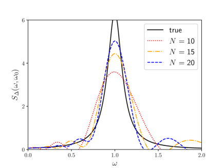
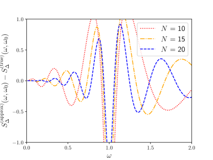
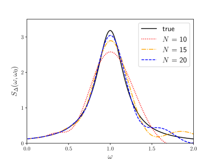
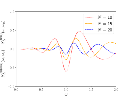
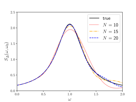
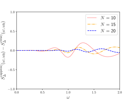
Figure 1: Left: Chebyshev approximation of the smearing kernel $S_{\Delta}(\omega,\omega_{0})$ for $\omega_{0}=1$ and $\Delta$ = 0.1 (top), 0.2 (middle) and 0.3 (bottom). Solid line is the true function, while dotted, dot-dashed and dashed lines are the approximations with $N$ = 10, 15 and 20, respectively. Right: Its error compared to the true function.

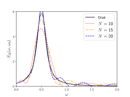
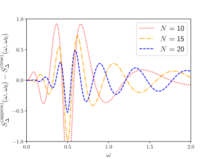
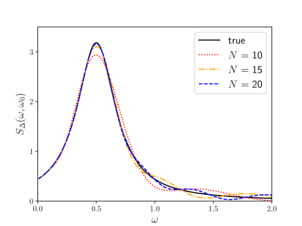
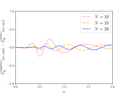
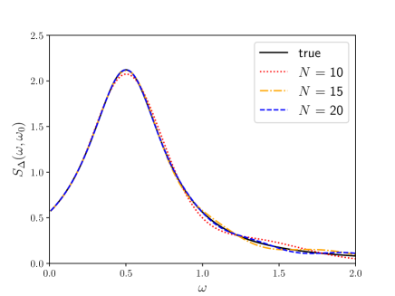
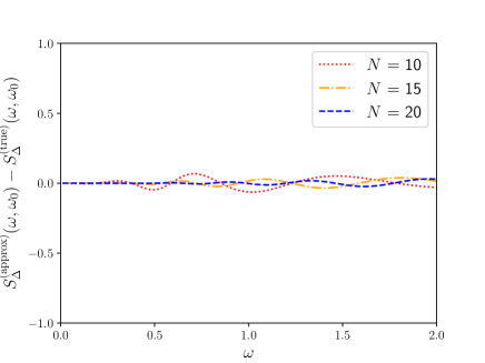
Figure 2: Same as Fig. 1 but for $\omega_{0}$ = 0.5.

In order to see the rate of convergence of the Chebyshev approximation, we plot the coefficients $c_{j}^{*}(\omega)$ as a function of $j$ in Fig. 3. As an example, the point $\omega=\omega_{0}$ is taken because this is where the error is largest. (It is not always the case especially when the approximation is already good. See Figs. 1 and 2.) One can see that the magnitude of the coefficient $|c_{j}^{*}(\omega)|$ decreases roughly exponentially as $j$. When the approximation is better (larger $\Delta$), the decrease of $|c_{j}^{*}(\omega)|$ is faster. Since the Chebyshev polynomial $|\langle T_{j}^{*}(\hat{z})\rangle|$ is bounded from above by 1, this shows (the upper limit of) the rate of convergence. The Calculation of $c_{j}^{*}(\omega)$ is numerically inexpensive, and one can easily estimate the error of the approximation due to a truncation at the order $N$ by $\pm|c_{N+1}^{*}(\omega)|$.

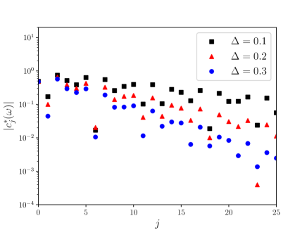
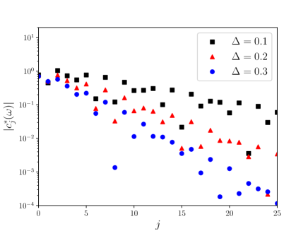
Figure 3: Coefficient of the Chebyshev approximation $c_{j}^{*}(\omega)$ at $\omega=\omega_{0}$ plotted against $j$ for $\omega_{0}$ = 1.0 (left) and 0.5 (right). Results for $\Delta$ = 0.1 (squares), 0.2 (triangles), and 0.3 (circles).

As another test, we consider the Laplace transform (4), which is achieved by a smearing kernel

$$S_{\rm Lap}(M^{2},\omega^{\prime})=\frac{2\omega^{\prime}}{M^{2}}e^{-\omega^{\prime 2}/M^{2}}.$$ (24)

In Fig. 4 we draw a curve of $S_{\rm Lap}(M^{2},\omega_{0})$, which represents a convolution with a trivial spectrum $\delta(\omega^{\prime}-\omega_{0})$, together with its approximations (22). The plots for $\omega_{0}$ = 1.0 (left) and 0.5 (right) demonstrate that the Chebyshev polynomials provide a very precise approximation even with $N$ = 10. This is not unreasonable because the Laplace transform is a smooth function over the entire range of energy.

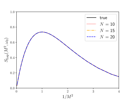
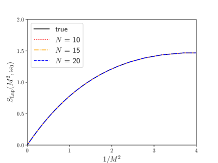
Figure 4: Chebyshev approximation of the kernel $S_{\rm Lap}(M^{2},\omega_{0})$ corresponding to the Laplace transform as a function of $1/M^{2}$. The true function (solid line) as well as its approximations (dotted, dot-dashed, dashed) are shown for $\omega_{0}$ = 1.0 (left) and 0.5 (right).

4 Smeared spectral function from lattice data: Charmonium correlators

We test the method with LQCD data for Charmonium correlators. Our data are obtained on the lattice with 2+1 flavors of Möbius domain-wall fermions. They have been previously used for an extraction of the charm quark mass from the Charmonium temporal moments Nakayama:2016atf . (The same lattice ensembles are also used for calculations of the Dirac spectrum Cossu:2016eqs ; Nakayama:2018ubk , short-distance current correlators Tomii:2017cbt , topological susceptibility Aoki:2017paw , $\eta^{\prime}$ meson mass Fukaya:2015ara .) Among 15 ensembles generated at various lattice spacings and lattice sizes, we use the one at a lattice spacing $a$ = 0.080 fm, a lattice size $32^{3}\times 64$, and bare quark masses $am_{ud}$ = 0.007 and $am_{s}$ = 0.040. The corresponding pion mass is 309(1) MeV. We take 100 gauge configurations and calculate the Charmonium correlator with a tuned charm quark mass $am_{c}$ = 0.44037, and compute charm quark propagators from $Z_{2}$ noises distributed over a time slice to construct Charmonium correlators. We then construct the Charmonium correlators, which correspond to those of local currents in the pseudo-scalar (PP) and vector (VV) channels. This calculation has been repeated for 8 source time slices to improve statistical signal, so that the total number of measurements is 800. Three spatial polarizations are averaged for the VV channel.

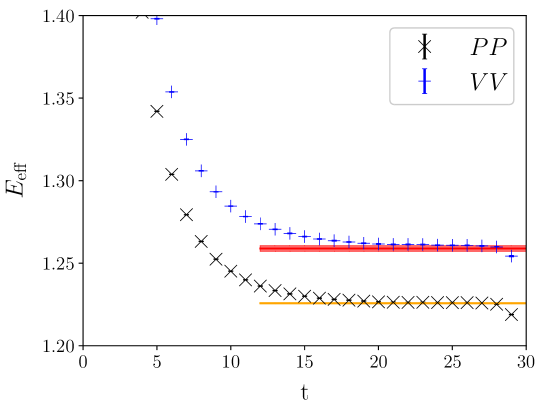
Figure 5: Effective mass of the pseudo-scalar (circles) and vector (squares) correlators calculated on the lattice with lattice cutoff $1/a$ = 2.453(4) GeV. The charm quark mass is tuned such that the spin-averaged 1S mass matches the experimental data.

Fig. 5 shows the effective mass $E_{\rm eff}(t)=\ln[C(t)/C(t+1)]$. We observe that the correlator is nearly saturated by the ground state at around $t=18$, and the information of the excited states are encoded in the region of smaller $t$’s. Energy levels and amplitudes obtained by a multi-exponential fit of the form $C(t)=\sum_{i}A_{i}e^{-E_{i}t}$ are given in Table 1. We include four levels in the fit, yet show the results only up to three levels since the error of the third amplitude is already large. Statistical correlation among different $t$’s is taken into account in the fit. The results reproduce the experimental data reasonably well. For instance, the lowest-lying vector meson masses are 3.09 and 3.76(19) GeV, which correspond to the experimentally observed $J/\psi$ and $\psi(2S)$ states of masses 3.10 and 3.69 GeV, respectively.

	PP channel		VV channel
$i$	$E_{i}$	$A_{i}$	$E_{i}$	$A_{i}$
0	1.22576(18)	0.17638(31)	1.2589(17)	0.1308(35)
1	1.521(19)	0.205(22)	1.534(79)	0.184(62)
2	1.831(15)	0.25(17)	1.834(15)	0.04(88)

Table 1: Energy levels and amplitudes for the Charmonium correlators.

We construct the Chebyshev matrix elements $\langle T_{j}^{*}(\hat{z})\rangle$ defined in (22) from the current correlators. The calculation is straightforward. Namely, we replace the term of $\hat{z}^{t}$ in the polynomials by $C(t+2t_{0})/C(2t_{0})$ and calculate the linear combinations of them with the coefficients of the shifted Chebyshev polynomials. We take $t_{0}=1$ in the lattice unit. The results are shown in Fig. 6; the error is calculated using the jackknife method. It turned out that the Chebyshev matrix elements are precisely determined up to $j=11$, which corresponds to $t=13$. Beyond that point, the statistical error grows rapidly, and the results eventually get out of the range of $\pm 1$, which must be satisfied for the Chebyshev polynomials.

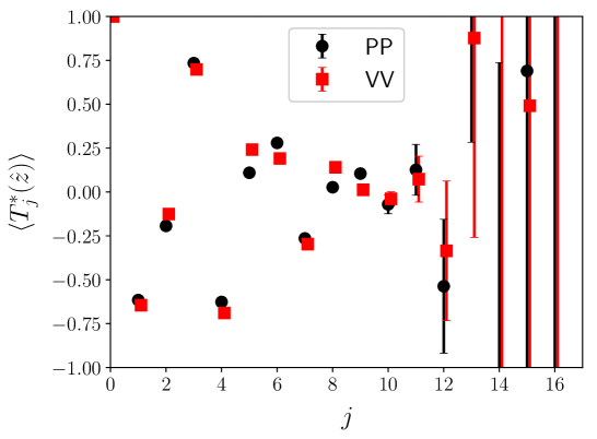
Figure 6: Chebyshev matrix elements $\langle T_{j}^{*}(\hat{z})\rangle$ for the PP (circles) and VV (squares) Charmonium correlators. The VV points are slightly shifted horizontally for clarity. The statistical error is estimated using the jackknife method.

In fact, the statistical error grows exponentially for higher-order polynomials as shown in Fig. 7. Its growth rate is about a factor of three to proceed by another order in $j$, which means that 10 times larger statistical samples would be needed to include yet another order to improve the Chebyshev approximation. This is not unreasonable because we try to construct the quantities of $O(1)$ as a linear combination of terms of exponentially different orders. For the Charmonium correlator at the lattice spacing chosen in this work, the terms of $\hat{z}^{t}$ are suppressed roughly by $e^{-1.2t}$, which is however compensated by the Chebyshev coefficients growing even faster. In the end, a strong cancellation among different powers of $\hat{z}$ gives a number between $-1$ and $+1$, and the noise is relatively enhanced. For instance, at the order $j=12$, a cancellation of four orders of magnitudes takes place and it becomes even harder for higher orders.

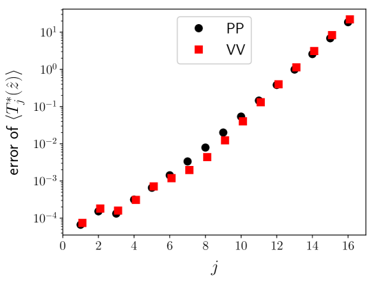
Figure 7: Statistical error of $\langle T_{j}^{*}(\hat{z})\rangle$ as a function of $j$. Circles and squares represent the data for PP and VV channels, respectively.

Since the Chebyshev approximation drastically fails outside the domain $0\leq x\leq 1$, we are not able to use it beyond the order where $|\langle T_{j}^{*}(\hat{z})\rangle|$ exceeds 1. Instead, we introduce a fit to determine these matrix elements $\bar{T}_{j}\equiv\langle T_{j}^{*}(\hat{z})\rangle$ in such a way that they are consistent with $\bar{C}(t)$ while satisfying a constraint $|\bar{T}_{j}|\leq 1$. To do so, we can use the reverse formula of the shifted Chebyshev polynomials Cheb_rev :

$$x^{n}=2^{1-2n}\sideset{}{{}^{\prime}}{\sum}_{r=0}^{n}\left(\begin{array}[c]{c}2n\\ n-r\end{array}\right)T_{r}^{*}(x),$$ (25)

where the prime on the sum indicates that the term of $r=0$ is to be halved. The relation to be satisfied is then

$$\bar{C}(t)=2^{1-2t}\left[\frac{1}{2}\left(\begin{array}[c]{c}2t\\ t\end{array}\right)+\sum_{r=1}^{t}\left(\begin{array}[c]{c}2t\\ t-r\end{array}\right)\bar{T}_{r}\right].$$ (26)

We take $T_{r}^{*}$’s as free parameters to be determined and fit the lattice data $\bar{C}(t)$ with a constraint $|\bar{T}_{j}|\leq 1$. Statistical correlations of $C(t)$ among different $t$’s are taken into account in the fit using the least-squares fit package lsqfit by Lepage lsqfit . The resulting values of $\bar{T}_{j}$ are listed in Table 2. Since the numbers of inputs, $\bar{C}(t)$’s, and unknowns, $\bar{T}_{j}$’s, are the same, the condition (26) may be solved as a system of linear equations unless the constraints are introduced. In fact, the results are unchanged from the direct determination through (2) within the statistical error for small $j$’s up to $j\simeq 10$. Beyond that, they are affected by the constraints. The error becomes large, of order 1, for large $j$’s, where they are essentially undetermined by the fit but still kept within $\pm 1$.

$j$	PP channel	VV channel
1	$-0.6157(17)$	$-0.6447(17)$
2	$-0.1933(48)$	$-0.1257(49)$
3	$0.7341(61)$	$0.6980(63)$
4	$-0.6262(46)$	$-0.6892(49)$
5	$0.1090(35)$	$0.2410(43)$
6	$0.2803(72)$	$0.1914(78)$
7	$-0.267(17)$	$-0.297(17)$
8	$0.036(38)$	$0.144(37)$
9	$0.073(81)$	$-0.001(78)$
10	$0.03(16)$	$0.01(15)$
11	$-0.14(26)$	$-0.08(25)$
12	$0.08(36)$	$0.07(35)$
13	$0.06(43)$	$0.03(42)$
14	$-0.07(51)$	$-0.05(51)$
15	$-0.05(60)$	$-0.02(59)$
16	$-0.01(77)$	$0.00(76)$

Table 2: Fit results for $\bar{T}_{j}$.

Once a set of estimates for $\langle T_{j}^{*}(\hat{z})\rangle$, i.e. $\bar{T}_{j}$, is obtained, the remaining task is to use (22) to estimate $\bar{\rho}_{\Delta}(\omega)$. The results are shown in Fig. 8. Three bands corresponding to the polynomial order $N$ = 12 (red), 14 (blue), 16 (orange) are overlaid. We find that the overall shape is unchanged by adding more terms, i.e. from 12 to 14 or to 16, while the size and shape of the statistical error is affected. When the polynomial order is lower, some wiggle structure is observed, while the necks, the positions of small statistical error, are fatten by adding more terms and eventually the error becomes nearly uniform over $\omega$. Beyond $N=16$, the results are essentially unchanged, since the higher order coefficients $c_{j}^{*}(\omega)$ are exponentially suppressed.

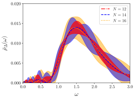
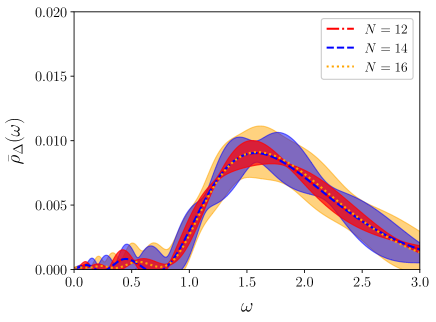
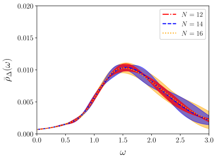
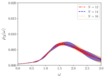
Figure 8: Smeared spectral function $\bar{\rho}_{\Delta}(\omega)$ reconstructed using (22). The order of approximation is $N$ = 12 (red), 14 (blue), 16 (orange). The results for $\Delta$ = 0.1 (top panels) and 0.3 (bottom panels), for the PP channel (left panels) and VV channel (right panels), are shown.

In Fig. 9 we show the results for the smeared spectral function $\bar{\rho}_{\Delta}(\omega)$ obtained with $N=16$. The smearing kernel is $S_{\Delta}(\omega,\omega^{\prime})$ with $\Delta$ = 0.1 (top), 0.2 (middle) and 0.3 (bottom). The results are compared with the expected contributions from the ground state and first excited state (red and blue curves). They are drawn assuming $\delta$-function distributions, $\bar{\rho}(\omega^{\prime})=\sum_{i}A_{i}e^{-\omega^{\prime}t_{0}}\delta(\omega^{\prime}-E_{i})$, with the fitted values of energy levels $E_{i}$ and their amplitudes $A_{i}$ given in Table 1. The factor $e^{-\omega^{\prime}t_{0}}$ is introduced to take account of the time evolution from 0 to $t_{0}$, which is included in the definition of the state $|\psi\rangle=e^{-Ht_{0}}J_{\mu}|0\rangle$.

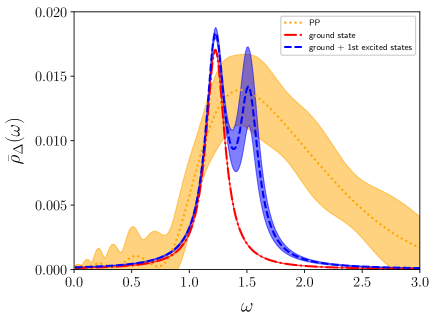
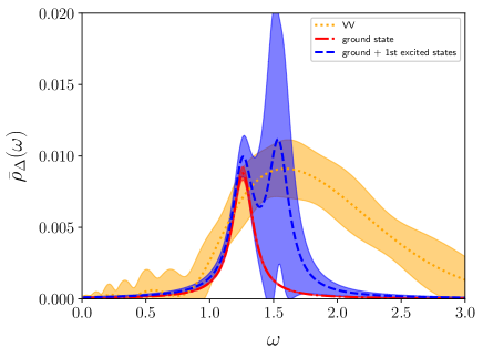
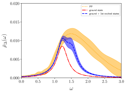
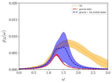
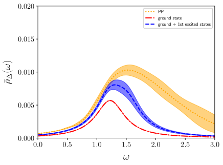
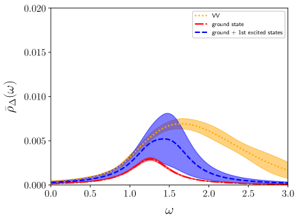
Figure 9: Reconstructed smeared spectral function $\rho_{\Delta}(\omega)$ for $\Delta$ = 0.1 (top), 0.2 (middle) and 0.3 (bottom). Left and right columns are those of the pseudo-scalar and vector channels. Results are shown by orange band, while the ground-state contribution (dot-dashed) and the ground-state and plus excited-state contribution (dashed) are plotted assuming they have $\delta$-function structures.

When the smearing width is large, $\Delta=0.3$ (bottom panels of Fig. 9), we observe that the reconstructed smeared spectral function follows the expected form from the low-lying states in the lower region of $\omega$. As $\omega$ increases, the spectral function indicates more contributions from higher excited states. This is exactly what we expected. The lattice data in the short time separations contain the information of such states, which is properly extracted with our method. From perturbation theory, one expects a constant proportional to the number of color degrees of freedom $N_{c}=3$ for the (unsmeared) spectral function $\rho(\omega)$. This constant is slightly distorted because of the difference between $\rho(\omega)$ and $\bar{\rho}(\omega)$. For $t_{0}=1$ (in the lattice unit), this should give an exponentially decreasing spectral function $\bar{\rho}_{\Delta}(\omega)$ as $\sim\omega^{2}e^{-2\omega}$ at large $\omega$, which is indeed observed in the results. On the other hand, the resonance structure is smeared out and invisible with $\Delta=0.3$ as one can see from the contributions of the ground and first-excited states.

For smaller smearing widths, $\Delta$ = 0.2 and 0.1, a larger systematic error is expected due to the truncation of the Chebyshev approximation. For $\Delta=0.2$, a typical size of the error is about 10–20% as one can see from Figures 1 and 2. (Dot-dashed lines correspond to $N=15$.) This error due to the truncation is not included in the band shown in Fig. 9, but taking account of this marginal size of error the reconstructed $\rho_{\Delta}(\omega)$ looks reasonable for $\Delta=0.2$ (middle panels). Namely, it follows the expected curve of the ground and the first excited states up to around the peak of the latter and then drops slowly due to higher excited state contributions.

The truncation error increases to 50–100% for $\Delta=0.1$ (upper panels of Figures 1 and 2), and we should not take the results (top panels of Fig. 9) too seriously. If it were precisely calculated, we would be able to resolve the resonance structures as the curve of the low-lying state contributions suggests. To do so, we need to include higher order terms of the Chebyshev approximation, which requires much better precision of the simulation data. This reflects the fact that the reconstruction of the full spectral function from Euclidean lattice data is an ill-posed problem. One needs ridiculously high precision in order to achieve a full reconstruction as emphasized in Hansen:2019idp .

5 Discussions

As already mentioned earlier, our proposal to calculate the smeared spectral function is not limited to the case just discussed. Any sort of weighted integral of the spectral function can be considered. A well-known example is the contribution of quark vacuum polarization to the muon anomalous magnetic moment $g-2$. Phenomenologically, one employs the optical theorem and dispersion relation to relate the vacuum polarization function in the Euclidean domain $\Pi(Q^{2})$ to a weighted integral of the experimentally observed $R$-ratio, or the spectral function. Then, an integral of $\Pi(Q^{2})$ with an appropriate weight gives the contribution to $g-2$. In this case, however, a direct expression in terms of the time correlator $C(t)$ is known Bernecker:2011gh , and we do not really need the approximation method developed in this work.

Another phenomenologically interesting example is the hadronic $\tau$ decay. Using the finite-energy sum rule Braaten:1991qm the hadronic width can be written as

$$R_{\tau}^{ud}=12\pi^{2}S_{\rm EW}|V_{ud}|^{2}\int_{0}^{m_{\tau}^{2}}\frac{ds}{m_{\tau}^{2}}\left(1-\frac{s}{m_{\tau}^{2}}\right)^{2}\left(1+\frac{2s}{m_{\tau}^{2}}\right)\rho_{V+A}(s),$$ (27)

where $S_{\rm EW}$ is a short-distance electroweak correction and $|V_{ud}|$ is a CKM matrix element. (Here, only the $ud$ contribution is considered. An extension to the $us$ contribution is straightforward.) The spectral function $\rho_{V+A}(s)$ denotes a sum of $VV$ and $AA$ channels. The integral (27) reflects a particular kinematics of $\tau$ decay and has a complicated form, but our method can be applied for such a case in principle. A practical question would be, however, whether a good enough approximation can be achieved with a limited number of terms.

The Laplace transform (24) is often considered in QCD sum rule analyses Shifman:1978bx because the corresponding Borel transform of perturbative series makes it more convergent. Our method allows to calculate two-point function after the Borel transform directly using lattice QCD. It may be useful to test the perturbative expansion and the operator product expansion involved in the QCD sum rule calculations. Conversely, it can also be used to validate lattice QCD calculations especially in the short-distance region. Such a test has been performed using short-distance correlators in the coordinate space Tomii:2017cbt , and it is interesting to do the test for the Borel transformed quantities.

The dispersion integral of the form (2) is of course another type of applications of our method. Although the vacuum polarization function $\Pi(Q^{2})$ in the space-like momenta $Q^{2}$ can be directly obtained by a Fourier transform of the lattice correlators, the Chebyshev approximation offers a method to extract it at arbitrary values of $Q^{2}$ corresponding to the momenta of non-integer multiples of $2\pi/L$. The Laplace transform as introduced in Feng:2013xsa can do this too, but requires the information of large time separations in the integral of the form $\int_{0}^{\infty}dt\,e^{\omega t}C(t)$. The method developed in this work accesses only to relatively short time separations, but we need to introduce an approximation. Systematic error in each case has to be carefully examined.

Extension to the cases of more complicated quantities, such as the nucleon structure function as measured in deep inelastic scattering or the inclusive hadron decays, can also be considered. One of the authors has proposed an analysis to use the dispersion integral to relate the inclusive decay rate to an amplitude in space-like momenta Hashimoto:2017wqo . This method contains a difficulty of requiring the information at unphysical momentum regions, which may be avoided by more flexible integral transformation proposed in this work.

For this class of applications, there are two independent kinematical variables, $q^{2}$ and $p\cdot q$, with $p$ the momentum of a decaying particle (or the initial nucleon) and $q$ the momentum transfer. In order to apply the method outlined in this work, we need to fix one of these kinematical variables and introduce a smearing on the other variable. More complicated integral might be useful for $b\to u\ell\nu$ decay analysis for which one introduces elaborate kinematical cuts in order to avoid backgrounds from $b\to c\ell\nu$. The flexibility of our method would allow such analyses.

Going to high tempertature QCD, our method would not work as it is, because the correlator can not be simply written as $\langle\psi|\hat{z}^{t}|\psi\rangle$ due to the contribution from the opposite time direction. The operator is then no longer a power of the transfer matrix, direct estimate of the Chebyshev matrix elements is not available.

6 Conclusions

Precise reconstruction of the spectral function from lattice data remains a difficult problem. Instead, we calculate a smeared counterpart, which contains some information of the spectral function after smearing out its detailed structures. For the Charmonium spectral function we obtain a reasonably precise result for a smearing width $\Delta$ = 0.3, which is about 700 MeV in the physical unit. Since the mass splittings experimentally observed are narrower than this, we are not able to resolve the details of the spectrum. Taking the limit of small smearing width requires exponentially better statistical precision, and it comes back to the original problem. Still, our proposal has advantages compared to previously available methods.

In contrast to the Bayesian approach Burnier:2013nla or the maximum entropy method Nakahara:1999vy ; Asakawa:2000tr , our method allows a reliable estimate of the systematic errors, since it does not assume any statistical distribution of unknown function. In principle, the method is deterministic once the input lattice data are given. The least-squared fit involved in order to enforce the constraint that eigenvalues of Hamiltonian is positive plays only a minor role that becomes irrelevant when the lattice data are made precise.

Compared to the Backus-Gilbert method Hansen:2017mnd , the method proposed in this paper is more flexible as it allows any predefined smearing function, while it is automatically determined in the Backus-Gilbert method and therefore is uncontrollable. The variant of the Backus-Gilbert method Hansen:2019idp also has this flexibility. Our method also allows systematic improvements since the approximation is achieved by a series of exponentially decreasing coefficients. As the statistical precision of the input correlator is improved, one can include higher order terms and thus improve the approximation.

The method can be used in the analysis of inclusive processes to define intermediate quantities for which fully non-perturbative lattice calculation is possible. Its potential application is not limited to the spectral function for two-point correlators, but other processes such as deep inelastic scattering and inclusive $B$ meson decays can be considered. Since the method does not rely on perturbation theory, the processes with small momentum transfer can be calculated on a solid theoretical ground, which was not available so far. More importantly, we do not have to rely on the assumption of quark-hadron duality.

References

- (1) Y. Nakahara, M. Asakawa and T. Hatsuda, Phys. Rev. D 60, 091503 (1999) doi:10.1103/PhysRevD.60.091503 [hep-lat/9905034].
- (2) M. Asakawa, T. Hatsuda and Y. Nakahara, Prog. Part. Nucl. Phys. 46, 459 (2001) doi:10.1016/S0146-6410(01)00150-8 [hep-lat/0011040].
- (3) Y. Burnier and A. Rothkopf, Phys. Rev. Lett. 111, 182003 (2013) doi:10.1103/PhysRevLett.111.182003 [arXiv:1307.6106 [hep-lat]].
- (4) L. Kades, J. M. Pawlowski, A. Rothkopf, M. Scherzer, J. M. Urban, S. J. Wetzel, N. Wink and F. Ziegler, arXiv:1905.04305 [physics.comp-ph].
- (5) M. T. Hansen, H. B. Meyer and D. Robaina, Phys. Rev. D 96, no. 9, 094513 (2017) doi:10.1103/PhysRevD.96.094513 [arXiv:1704.08993 [hep-lat]].
- (6) M. Hansen, A. Lupo and N. Tantalo, Phys. Rev. D 99, no. 9, 094508 (2019) doi:10.1103/PhysRevD.99.094508 [arXiv:1903.06476 [hep-lat]].
- (7) R. A. Tripolt, P. Gubler, M. Ulybyshev and L. Von Smekal, Comput. Phys. Commun. 237, 129 (2019) doi:10.1016/j.cpc.2018.11.012 [arXiv:1801.10348 [hep-ph]].
- (8) E. C. Poggio, H. R. Quinn and S. Weinberg, Phys. Rev. D 13, 1958 (1976). doi:10.1103/PhysRevD.13.1958
- (9) R. A. Bertlmann, G. Launer and E. de Rafael, Nucl. Phys. B 250, 61 (1985). doi:10.1016/0550-3213(85)90475-4
- (10) M. A. Shifman, A. I. Vainshtein and V. I. Zakharov, Nucl. Phys. B 147, 385 (1979). doi:10.1016/0550-3213(79)90022-1
- (11) D. Bernecker and H. B. Meyer, Eur. Phys. J. A 47, 148 (2011) doi:10.1140/epja/i2011-11148-6 [arXiv:1107.4388 [hep-lat]].
- (12) K. Nakayama, B. Fahy and S. Hashimoto, Phys. Rev. D 94, no. 5, 054507 (2016) doi:10.1103/PhysRevD.94.054507 [arXiv:1606.01002 [hep-lat]].
- (13) G. Cossu, H. Fukaya, S. Hashimoto, T. Kaneko and J. I. Noaki, PTEP 2016, no. 9, 093B06 (2016) doi:10.1093/ptep/ptw129 [arXiv:1607.01099 [hep-lat]].
- (14) K. Nakayama, H. Fukaya and S. Hashimoto, Phys. Rev. D 98, no. 1, 014501 (2018) doi:10.1103/PhysRevD.98.014501 [arXiv:1804.06695 [hep-lat]].
- (15) M. Tomii et al. [JLQCD Collaboration], Phys. Rev. D 96, no. 5, 054511 (2017) doi:10.1103/PhysRevD.96.054511 [arXiv:1703.06249 [hep-lat]].
- (16) S. Aoki et al. [JLQCD Collaboration], PTEP 2018, no. 4, 043B07 (2018) doi:10.1093/ptep/pty041 [arXiv:1705.10906 [hep-lat]].
- (17) H. Fukaya et al. [JLQCD Collaboration], Phys. Rev. D 92, no. 11, 111501 (2015) doi:10.1103/PhysRevD.92.111501 [arXiv:1509.00944 [hep-lat]].
- (18) J. López-Bonilla, E. Ramírez-García, C. Sosa-Caraveo, Revista Notas de Matemática, Vol.6(1), 287 (2010) 18.
- (19) G.P. Lepage, lsqfit, https://github.com/gplepage/lsqfit
- (20) E. Braaten, S. Narison and A. Pich, Nucl. Phys. B 373, 581 (1992). doi:10.1016/0550-3213(92)90267-F
- (21) X. Feng, S. Hashimoto, G. Hotzel, K. Jansen, M. Petschlies and D. B. Renner, Phys. Rev. D 88, 034505 (2013) doi:10.1103/PhysRevD.88.034505 [arXiv:1305.5878 [hep-lat]].
- (22) S. Hashimoto, PTEP 2017, no. 5, 053B03 (2017) doi:10.1093/ptep/ptx052 [arXiv:1703.01881 [hep-lat]].