Binary Classification with XOR Queries:
Fundamental Limits and An Efficient Algorithm

Abstract

We consider a query-based data acquisition problem for binary classification of unknown labels, which has diverse applications in communications, crowdsourcing, recommender systems and active learning. To ensure reliable recovery of unknown labels with as few number of queries as possible, we consider an effective query type that asks “group attribute” of a chosen subset of objects. In particular, we consider the problem of classifying $m$ binary labels with XOR queries that ask whether the number of objects having a given attribute in the chosen subset of size $d$ is even or odd. The subset size $d$, which we call query degree, can be varying over queries. We consider a general noise model where the accuracy of answers on queries changes depending both on the worker (the data provider) and query degree $d$. For this general model, we characterize the information-theoretic limit on the optimal number of queries to reliably recover $m$ labels in terms of a given combination of degree-$d$ queries and noise parameters. Further, we propose an efficient inference algorithm that achieves this limit even when the noise parameters are unknown.

I Introduction

Binary classification is one of the most fundamental problems in engineering and appears in a wide variety of fields such as communication, machine learning [2], recommender systems, crowdsourcing [3], and VLSI systems [4]. In data acquisition for binary classification, one often acquires noisy answers from queries on the unknown binary labels, and by applying an inference algorithm the true labels are recovered. The common goal of such a data acquisition problem is to reliably recover the true labels at the minimum sample complexity (the number of queries). To achieve this goal, an efficient querying strategy needs to be designed. There also exist some cases where we do not have a freedom to design queries, but rather it is directly inherited from the application. Designing a statistically-efficient inference algorithm is also important to fully exploit the information from answers so as to minimize the sample complexity, but at the same time, the algorithm should have affordable computational complexity to be used in large-scale problems.

Different types of queries have been studied, regarding different properties of target applications. For example, many literatures on crowdsourcing have investigated the most basic querying method named repetition query that asks one label at a time repeatedly to many workers [5, 6, 7, 8]. More complex querying method such as pairwise comparison [9] asking whether or not two objects belong to the same class, or “triangle” queries [10], which compare three objects simultaneously, were considered to increase the statistical-efficiency in answers. Pairwise comparison was also studied extensively through the stochastic block model [11], which is a standard model for studying community recovery problems in graphs. The homogeneity measurement that extends pairwise comparison to the hypergraph case to measure the homogeneity of more than two nodes was further investigated in some previous works [12, 13, 14].

In this work, we focus on the XOR-based querying method, which asks whether the number of objects having a given attribute in the chosen subset of size (degree) $d$ is even or odd. Binary classification with XOR queries has long been studied in the context of linear codes in channel coding [15, 16, 17], XOR-based hypergraph clustering [13], and random XOR-constrained satisfaction problem [18] with applications in statistical physics [19]. We study this problem in a very general setup where the error probability of the answers as well as the subset size $d$ is non-uniform over queries. We assume that the queries are answered by many workers having different error probabilities although each worker answers the queries of the same $d$ uniformly with assigned error probability. The terminology “worker” is inspired by the crowdsourcing system [3], but it can be considered as different channels through which the data is transmitted, or different environments that affect the edge generation probability of a hypergraph. We additionally assume that the error probabilities of workers are unknown to reflect the scenarios, in crowdsourcing where worker reliabilities are unknown a priori, or in communication systems where the channel condition varies over time. Lastly, the assumption of non-uniform $d$ allows very general setups in the corresponding problems where we obtain measurements over different number of objects interacting with each other.

I-A Main Contributions

In this work, we provide rigorous and general analysis of XOR queries in binary classification and demonstrate the sample efficiency of this type of querying strategy. We derive a sharp threshold on the required number of queries to recover $m$ binary labels in terms of a given combination of degree-$d$ XOR queries and worker noise parameters. Further, we provide an efficient inference algorithm to extract correct labels from the noisy answers of XOR queries, which achieves the information-theoretic limit even when the noise parameters are unknown.

Concretely, when the fraction of degree-$d$ queries is $\Phi_{d}\in[0,1]$ for $d\in\{1,\dots,D\}$ and the probability that a worker $k$ provides an incorrect answer to a degree-$d$ query is $\epsilon_{k,d}<1/2$, we show in Theorem 1 that the number of queries should be at least

$$n=\frac{m\log m}{\sum_{d=1}^{D}\sum_{k=1}^{w}\frac{d\Phi_{d}}{w}(\sqrt{1-\epsilon_{k,d}}-\sqrt{\epsilon_{k,d}})^{2}}$$ (1)

to recover all $m$ binary labels with high probability as $m\to\infty$, where the maximum query degree is $D=\Theta(1)$ and each query is assigned to a worker chosen uniformly at random among total $w$ workers. We provide both upper and lower bounds that deviate only by an arbitrary small constant factor from (1). The upper and lower bounds are derived by analyzing the optimal maximum likelihood (ML) decoder with the knowledge of worker noise parameters $\{\epsilon_{k,d}\}$.

Our main contribution is on proposing an efficient inference algorithm that achieves the optimal sample complexity for any combination of the query degree $d$’s even when the worker noise parameters $\{\epsilon_{k,d}\}$ are unknown. The main idea is to boost the accuracy of our estimates on the correct labels by three steps, where the worker noise parameters are estimated after the first two steps and then used to refine the estimates on labels at the last step. More specifically, we show that the weak recovery of labels (of which the formal definition will be provided in the next section) is possible without estimating the worker noise parameters by relying on one-step message passing and majority voting. The worker noise parameters can be estimated up to a desired accuracy based on the weakly recovered labels. Finally, the strong recovery of labels (of which the formal definition will be provided in the next section) is achieved by the weighted majority voting with the estimated noise parameters. The proposed algorithm is inspired by the recent two-step estimation approaches, which have been used in clustering or non-convex estimation problems, where the initial estimate, which is close to the solution up to a certain limit, is provided by some classical technique (e.g. spectral method) and the refinement step (e.g. gradient descent) is followed to boost the accuracy of the estimate [20, 21, 11].

One important assumption posed on our algorithm is the presence of $\Theta(m)$ degree-1 queries. It is used to construct an initial estimate that makes our algorithm to move toward the correct direction. In applications of data acquisition where one can design querying strategy, this is a natural assumption. On the other hand, in other applications where degree-1 queries are unavailable, the degree-1 queries can be viewed as some sort of side information that provides an initial estimate that is better than random guess. Hence, the assumption can be related to the recent research direction where side information is used to help solve the original problem with smaller sample complexity [22, 23, 24].

We show that the proposed algorithm guarantees the recovery of $m$ labels at the optimal sample complexity provided by (1) as $m\to\infty$ even when the worker noise parameters are unknown (Theorem 2). We provide some experimental results with synthetic data that support our theoretical findings. In particular, to fairly compare the XOR quires of different degrees and with other types of queries, we consider an error model called $d$-coin flip model. We also apply our algorithm to crowdsourced binary classification with the data collected from Amazon Mechanical Turk and show the effectiveness of XOR query in reducing the sample complexity.

I-B Related Works

I-B1 Constraint Satisfaction Problem

The recovery of $m$ binary labels from noisy XOR queries can be viewed as an example of a planted constraint satisfaction problem (CSP), which is a subject of intense study in computer science, probability theory, and statistical physics, motivated by clustering, community detection, and cryptographic applications. Consider in particular a random planted $d$-XORSAT problem, where the goal is to recover $m$ binary variables (the planted solution) satisfying a set of $n$ constraints such that XOR of size-$d$ subsets of variables should be equal 0 (or 1) where the subsets are chosen uniformly at random among $m\choose d$ possibilities. This is the same recovery problem as ours except that for our setup, the subset size $d$ can be varying over constraints and the XOR value can be noisy. There have been many works [25, 26, 27] to answer 1) how large $n$ should be to make the planted solution a unique solution, and 2) how large $n$ should be for the planted solution recoverable by an efficient algorithm. When $d=3$, this problem is also a special case of tensor completion problems, and the best known algorithm with polynomial-time complexity requires $n=\Omega(m^{3/2})$ [28]. In this work, we show that by adding $\Theta(m)$ degree-1 queries, which does not change the order of sample complexity, the optimal sample complexity of $\Theta(m\log m)$ is achievable by an efficient algorithm of $O(m\log m)$ time steps.

I-B2 Hypergraph Clustering

The problem we consider also has close connections to the XOR-based hypergraph clustering problem [13, 25, 29]. The goal of hypergraph clustering is to classify nodes (binary labels) by using randomly sampled XOR measurements among ${m\choose d}$ possibilities on subsets of node labels. The main difference from our model is that in the hypergraph clustering the subset size $d$ is often fixed as a constant and each hyperedge in the set of size ${m\choose d}$ is independently sampled (without replacement) with a fixed probability $p$ (thus the number of total measurements is a random variable distributed by $\text{Binomial}({m\choose d},p)$.) Also, the error probability is often identical over the measurements. In our model, on the other hand, we can design queries so that for each query we randomly choose the query degree $d$ and select $d$ labels among $m$ uniformly at random. The error probability of each query may also depend on the query degree and the worker. In [13], the necessary and sufficient conditions on the expected number of hyperedge measurements $p{m\choose d}$ were analyzed and shown to be $\frac{m\log m}{d(\sqrt{1-\epsilon}-\sqrt{\epsilon})^{2}}$. In our work, we generalize this result for our measurement model (where the number $n$ of queries is fixed and each query is randomly designed and assigned to one of workers in the system) and show that (1) is the necessary and sufficient number of queries to recover all the $m$ labels reliably. Addition to this theoretical analysis, the main contribution of our work is that we provide the almost linear-complexity inference algorithm (up to logarithmic factor) with which we can infer all the $m$ labels with high probability even when the error parameters of the workers are unknown.

I-B3 Linear Codes

The result of this work can be applied to communication systems by viewing XOR queries as a linear code for binary labels. The randomly generated XOR queries correspond to the scenario where a receiver has no control over what packets to receive and just receives random $n$ packets from the transmitter (as in rateless coding setup with fountain codes [16]). Also, the workers in our model can be thought of as many different channels with unknown error probabilities as in [30, 31]. The degree constraint $D=\Theta(1)$ for the coded bits can be motivated from locally encodable coding [32]: a data compression/transmission problem where each coded bit depends only on a small number of input bits.

I-B4 Crowdsourcing

Crowdsourcing systems usually rely on simple querying types that human workers are easy to answer. However, information efficiency of such simple query types is often limited; all the simple query types including repetition query [3], pairwise comparison [9], and homogeneity measurement [13] require larger sample complexity than the degree-3 XOR querying scheme under the same error probability. However, XOR queries are relatively harder to answer for human workers, so that the corresponding error rate in the answers may increase in practice. Hence, it is worth investigating whether the gain in sample complexity can offset the loss from the increased error rate of XOR queries in real crowdsourcing systems. Our experimental result provided in Section V answers this question in an affirmative way, and opens a possibility for XOR queries to be used in crowdsourced classification.

I-C Organization of the Paper

The rest of the paper is organized as follows. In Section II, we formulate the binary classification problem with XOR query for a general noise model where the accuracy of worker’s answer changes depending both on the worker reliability and query degree $d$. Section III provides the information-theoretic limits on the required number of queries to recover all the labels with high probability, in terms of a given combination of degree-$d$ queries and worker noise parameters. In Section IV, we present our computationally-efficient algorithm that achieves the information-theoretic limit on the optimal number of queries, even without the knowledge of worker noise parameters. In Section V, we present simulation results that demonstrate the effectiveness of XOR querying strategy and the proposed inference algorithm compared to existing crowdsourcing strategies both for synthetic and real datasets. Section VI provides proofs on the performance of the proposed algorithm. Section VII provides conclusions with future research directions. Technical proof details on the main results can be found in appendices.

I-D Notations

We denote a vector by a bold face letter, e.g. $\mathbf{v}$, and the $i$-th component of it by $v_{i}$. Both of Bernoulli distribution (value 0 or 1) and Rademacher distribution (value $-1$ or $1$) with parameter $p$ are denoted by $\text{Bern}(p)$. We use $[n]$ to denote $\{1,2,\cdots,n\}$, and for any set $A$, $|A|$ is the number of elements in $A$. We define the function $\operatorname{sgn}(x)$ as $1$ if $x>0$, $-1$ if $x<0$, and $1$ with probability 1/2 and $-1$ with probability 1/2 if $x=0$. Also, the function $\textsf{TRUNC}(x,I)$ is defined as the element in the interval $I$ that is closest to $x$.

II Model

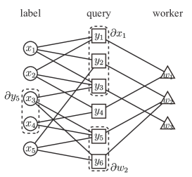
Figure 1: A tripartite graph depicting query design and worker assignment. The figure is drawn for the case where the query degrees are either $d=2$ or $d=3$.

Let $\mathbf{x}\in\{1,-1\}^{m}$ be the ground truth label vector we aim to recover and $\widehat{\mathbf{x}}\in\{1,-1\}^{m}$ be the estimate of the label vector. We ask in total of $n$ queries to $w$ workers, and $\mathbf{y}\in\{1,-1\}^{n}$ denotes a collection of all answers we get from the workers. There are three notions of recovery used in this paper. Strong recovery refers to the case where $\mathbf{x}$ itself is recovered perfectly with high probability as $m\to\infty$, i.e., $\operatorname*{\mathbb{P}}\left[\widehat{\mathbf{x}}\neq\mathbf{x}\right]\to 0$. Weak recovery is the case where the error probability of each $x_{i}$ goes to 0 for all $i\in[m]$, i.e., $\operatorname*{\mathbb{P}}\left[\widehat{x}_{i}\neq x_{i}\right]\to 0$. When the error probability of each $x_{i}$ is better than random guess, i.e., $\operatorname*{\mathbb{P}}\left[\widehat{x}_{i}\neq x_{i}\right]<{1}/{2}$ for all $i\in[m]$, we say that detection is possible.

II-A Query Design and Assignment

Each query is designed independently by first obtaining a query degree $d$ from a probability distribution ${{\Phi}}=\{\Phi_{1},\dots,\Phi_{D}\}$ and then selecting $d$ components of $\mathbf{x}$, which will be contained in the query, uniformly at random among ${m\choose d}$ possibilities. We assume that both the maximum query degree $D$ and the degree distribution $\Phi_{D}$ do not scale with $m$. Each query asks XOR of the $d$ labels to a worker chosen uniformly at random among total $w$ workers. Note that we are considering the non-adaptive model; all queries are designed in advance of getting any answer from the workers.

II-B Tripartite Graph Representation

A tripartite graph is used to describe the query design and the worker assignment for each query as in Figure 1. We use indices $i\in[m],j\in[n],k\in[w]$ for label, query, worker nodes, respectively. Let $\partial x_{i}\subset[n]$ denote the set of queries that contain the label $x_{i}$, and $\partial y_{j}\subset[m]$ denote the set of labels that are contained in the $j$-th query. Also, let $\partial w_{k}\subset[n]$ denote the set of queries that are assigned to the worker $k\in[w]$. When $A\subset[n]$ is a subset of queries, denote by $A_{d}:=\{j\in A:|\partial y_{j}|=d\}$ the degree-$d$ queries in the set $A$. Then, the set $\partial x_{i}\cap A_{d}$ includes the degree-$d$ queries in $A$ that are connected to the label node $x_{i}$, and the set $\partial w_{k}\cap A_{d}$ includes the degree-$d$ queries in $A$ that are assigned to the worker $k$. For the $j$-th query, the assigned worker and the query degree are denoted by $w(j)$ and by $d(j)$, respectively.

II-C Noise Model

In order to study the problem in full generality, we assume that the error probabilities of the workers are not uniform and also depend on the query degree. In particular, we assume that the worker $k$ gives a wrong answer with probability $\epsilon_{k,d}\in[\lambda,0.5)$ when answering a degree-$d$ XOR query, where $\lambda>0$ is an arbitrary small constant. Hence, there is no perfectly reliable worker, i.e., $\epsilon_{k,d}>0$. This is a technical assumption though to make the weight $\log\frac{1-\widehat{\epsilon}_{k,d}}{\widehat{\epsilon}_{k,d}}$, which is used for a weighted majority voting in a step of our proposed inference algorithm, not diverge by bounding $\widehat{\epsilon}_{k,d}\geq\lambda$ where $\widehat{\epsilon}_{k,d}$ is the estimate worker reliability.

III Information-Theoretic Bounds on the Optimal Sample Complexity

We first analyze the optimal number of queries (the sample complexity) for the strong recovery of the label vector ${\mathbf{x}}$, i.e., to guarantee $\operatorname*{\mathbb{P}}\left[\widehat{\mathbf{x}}\neq\mathbf{x}\right]\to 0$ as $m\to\infty$, in terms of a given fraction of degree-$d$ queries $\{\Phi_{1},\dots,\Phi_{D}\}$ and the noise parameters $\{\epsilon_{k,d}\}$ for $k\in[w]$ and $d\in[D]$. We derive necessary and sufficient conditions on the sample complexity $n$ when the noise parameters $\{\epsilon_{k,d}\}$ of workers’ answers are known at the inference algorithm. Thus, this result provides a lower bound on the optimal sample complexity for the case when $\{\epsilon_{k,d}\}$ is unknown, which is a more practical situation for applications such as crowdsourcing systems. In the next section, we develop an inference algorithm that does not require a prior knowledge of $\{\epsilon_{k,d}\}$ but still achieves the information-theoretic limit of the known $\{\epsilon_{k,d}\}$ case.

Theorem 1.

Assume that total $n$ XOR queries are randomly and independently generated among which the fraction of degree-$d$ queries is $\Phi_{d}\geq 0$ for $\sum_{d=1}^{D}\Phi_{d}=1$ and $\sum_{d\text{ odd}}\Phi_{d}>0$. Each query is randomly assigned to a worker $k\in[w]$ who provides an incorrect answer to a degree-$d$ query with probability $0<\epsilon_{k,d}<1/2$. With the maximum likelihood (ML) estimator $\widehat{\mathbf{x}}\in\{1,-1\}^{m}$, which minimizes $\operatorname*{\mathbb{P}}\left[\widehat{\mathbf{x}}\neq\mathbf{x}\right]$ for a known $\{\epsilon_{k,d}\}$, the strong recovery is possible, i.e., $\operatorname*{\mathbb{P}}\left[\widehat{\mathbf{x}}\neq\mathbf{x}\right]\to 0$ as $m\to\infty$, if the number of queries is

$$n\geq(1+\eta)\frac{m\log m}{\sum_{d=1}^{D}\sum_{k=1}^{w}\frac{d\Phi_{d}}{w}(\sqrt{1-\epsilon_{k,d}}-\sqrt{\epsilon_{k,d}})^{2}},$$ (2)

and only if

$$n\geq(1-\eta)\frac{m\log m}{\sum_{d=1}^{D}\sum_{k=1}^{w}\frac{d\Phi_{d}}{w}(\sqrt{1-\epsilon_{k,d}}-\sqrt{\epsilon_{k,d}})^{2}},$$ (3)

for any arbitrarily small constant $\eta>0$.

Proof:

The proof of this theorem is provided in Appendix A. ∎

Remark 1 (Efficiency of high-degree XOR queries).

For a special case where the worker error probability is independent of the query degree $d$, i.e., $\epsilon_{k,d}=\epsilon_{k}$, Theorem 1 shows that the sample complexity is inversely proportional to the average query degree $\sum_{d=1}^{D}d\Phi_{d}$ when $D=\Theta(1)$. This implies that increasing the query degree and asking a more complicated query to a worker helps reduce the required number of queries, if the error probability of a worker’s answer does not change depending on the complexity of the queries.

Remark 2 (Optimal degree of XOR queries for a general error model).

For a general set of $\{\epsilon_{k,d}\}$, it can be inferred from (2) that concentrating the degree distribution to a degree that has the maximum value of $\sum_{k=1}^{w}d(\sqrt{1-\epsilon_{k,d}}-\sqrt{\epsilon_{k,d}})^{2}$ would be the optimal way to minimize the required number of queries. In other words, the optimal query degree that minimizes the required number of queries is $d^{*}=\operatorname*{argmax}_{d\in\{1,\dots,D\}}\sum_{k=1}^{w}d(\sqrt{1-\epsilon_{k,d}}-\sqrt{\epsilon_{k,d}})^{2}$. However, in many applications, the query designer has no knowledge on the workers’ reliabilities $\{\epsilon_{k,d}\}$ at the stage of query design, so determining the optimal query degree in advance is impossible. This motivates a query designer to mix queries with different degrees. A more important aspect of mixing queries with different degrees we argue in this paper is that it is possible to achieve the optimal sample complexity (2) with an efficient algorithm even when $\{\epsilon_{k,d}\}$ is unknown, if there exist $\Theta(m)$ number of degree-1 queries. Thus, in the next section we will assume that the degree of the first $m$ queries is fixed to 1 regardless of the query-degree distribution $\Phi$. Note that the addition of $m$ queries has negligible effect on the optimal sample complexity, which scales as $\Theta(m\log m)$. More details will be found in the next section where we propose an efficient inference algorithm.

Remark 3 (Comparison to homogeneous query).

The homogeneous query, which asks whether all the items in a chosen subset of size $d$ belong to the same class or not, is another widely-studied group-query type. In [13], the required number of measurements to recover $m$ binary labels from random homogeneous query of degree-$d$ was analyzed in the context of hypergraph clustering. The paper considered the setup where the query degree and the error probability are fixed to $d$ and $\epsilon$, respectively, for all the queries. Under such a setup, it was shown that the required number of measurements (the answers from random homogeneous query) for strong recovery of $m$ binary labels scales as $\frac{2^{d-2}}{d}\frac{m\log m}{(\sqrt{1-\epsilon}-\sqrt{\epsilon})^{2}}$. Note that the information efficiency of homogeneous query decreases as the query degree $d$ increases; whereas that of XOR query increases as in (2), as long as the error probability of workers’ answer does not increase too fast to offset the information gain from the increased query degree. In Section V, we provide simulation results to compare the information efficiency of XOR query, homogeneous query as well as repetition query under a fair error-model called $d$-coin flip model.

IV An Efficient Algorithm Achieving the Optimal Sample Complexity

In this section, we propose a computationally-efficient algorithm that guarantees the strong recovery of $m$ binary labels at the optimal sample complexity (2) even when the worker reliabilities $\{\epsilon_{k,d}\}$ are unknown. We assume that the first $m$ queries have a fixed degree $d=1$ and ask each of the $m$ labels exactly once.

IV-A Four-Phase Inference Algorithm for XOR Queries

Algorithm 1 Four-Phase Inference Algorithm for XOR Queries

1:  Data: The observed query answers $\mathbf{y}\in\{1,-1\}^{n}$ and the tripartite graph (as in Fig. 1) depicting query design and worker assignment.

2:  Phase 1. (Detection of labels): Let $A^{(1)}$ be the set of first $m$ degree-1 queries asking each label. For each label $i\in[m]$, calculate the first estimate of $x_{i}$ as

$$\widehat{x}_{i}^{(1)}=\operatorname{sgn}(y_{j_{i}}),$$ (4)

where $j_{i}=\partial x_{i}\cap A^{(1)}$.

3:  Phase 2. (Weak recovery of labels): Let $A^{(2)}$ be the next $n^{(2)}=m\left(\frac{\log m}{\log\log m}\right)$ queries. For each label $i\in[m]$ and query $j\in\partial x_{i}\cap A^{(2)}$, let $m_{j\to i}^{(2)}=y_{j}\prod_{i^{\prime}\in\partial y_{j}\backslash\{i\}}\widehat{x}_{i^{\prime}}^{(1)},$ and calculate the second estimate of $x_{i}$ as

$$\widehat{x}_{i}^{(2)}=\operatorname{sgn}\Bigg{(}\sum_{j\in\partial x_{i}\cap A^{(2)}}m_{j\to i}^{(2)}\Bigg{)}.$$ (5)

4:  Phase 3. (Estimating workers’ reliabilities): Let $A^{(3)}$ be the next $n^{(3)}=w(\log m)(\log\log m)$ queries. For each query $j\in A^{(3)}$, define $E_{j}^{(3)}=\mathds{1}\bigg{(}y_{j}\neq\prod_{i\in\partial y_{j}}\widehat{x}_{i}^{(2)}\bigg{)}.$ For each worker $k\in[w]$ and degree $d\in[D]$, choose the estimate of the noise parameter $\epsilon_{k,d}$ as

$$\widehat{\epsilon}_{k,d}=\textsf{TRUNC}\left(\frac{\sum_{j\in\partial w_{k}\cap A_{d}^{(3)}}E_{j}^{(3)}}{|\partial w_{k}\cap A_{d}^{(3)}|},[\lambda,0.5]\right).$$ (6)

5:  Phase 4. (Strong recovery of labels): Let $A^{(4)}$ be the rest $n^{(4)}=n-n^{(1)}-n^{(2)}-n^{(3)}$ queries. For each label $i\in[m]$ and query $j\in\partial x_{i}\cap A^{(4)}$, let $m_{j\to i}^{(4)}=y_{j}\prod_{i^{\prime}\in\partial y_{j}\backslash\{i\}}\widehat{x}_{i^{\prime}}^{(2)}$ and $M_{j\to i}^{(4)}=\log\bigg{(}\frac{1-\widehat{\epsilon}_{w(j),d(j)}}{\widehat{\epsilon}_{w(j),d(j)}}\bigg{)}m_{j\to i}^{(4)},$ and calculate the final estimate of $x_{i}$ as

$$\widehat{x}_{i}^{(4)}=\operatorname{sgn}\Bigg{(}\sum_{j\in\partial x_{i}\cap A^{(4)}}M_{j\to i}^{(4)}\Bigg{)}.$$ (7)

6:  Output: Final estimates $\widehat{\mathbf{x}}:=\widehat{\mathbf{x}}^{(4)}$ for labels.

The algorithm we propose, presented as Algorithm 1, is composed of four phases: detection of labels, weak recovery of labels, estimation of workers’ reliabilities, and strong recovery of labels. We divide the total queries of size $n$ into four sets $A^{(1)}$, $A^{(2)}$, $A^{(3)}$, and $A^{(4)}$ of sizes $|A^{(1)}|=m$, $|A^{(2)}|=m\frac{\log m}{\log\log m}$, $|A^{(3)}|=w(\log m)(\log\log m)$, and $|A^{(4)}|=n-\sum_{l=1}^{3}|A^{(l)}|$, and use each set only at the corresponding phase of the algorithm. We assume that the set $A^{(1)}$ is composed of only degree-1 queries each of which asks each label $i\in[m]$. The key intuition underlying Algorithm 1 is as follows.

• At Phase 1, we make an initial guess on each label $i\in[m]$ by using the $m$ degree-1 queries in $A^{(1)}$. When $y_{j_{i}}$ is the answer for the label $x_{i}$, we define the initial estimate of $x_{i}$, denoted by $\widehat{x}_{i}^{(1)}$, to be equal to $\operatorname{sgn}(y_{j_{i}})$. Since we assume $\epsilon_{k,d}<1/2$ regardless of the worker $k$, the answer is better than a random guess and we can guarantee the detection of all the labels from this step, i.e., $\operatorname*{\mathbb{P}}\left[\widehat{x}^{(1)}_{i}\neq x_{i}\right]<{1}/{2}$ for all $i\in[m]$. This initial phase helps our estimates on the following phases converge toward the correct labels, and without this phase, the following phases could be nothing more than a random guess.

• At Phase 2, we use the estimates $\{\widehat{x}_{i}^{(1)}\}$ from Phase 1 and the next set of $m\left(\frac{\log m}{\log\log m}\right)$ queries in $A^{(2)}$ to generate the second estimates $\{\widehat{x}_{i}^{(2)}\}$ for the labels. Each query node $j\in\partial x_{i}\cap A^{(2)}$ transmits a ‘message’ $m_{j\to i}^{(2)}=y_{j}\prod_{i^{\prime}\in\partial y_{j}\backslash\{i\}}\widehat{x}_{i^{\prime}}^{(1)}\in\{1,-1\}$ to its neighboring label node $i$, where the message is the estimate of $x_{i}$ based on the query answer $y_{j}$ and the estimates $\{\widehat{x}_{i^{\prime}}^{(1)}:{i^{\prime}\in\partial y_{j}\backslash\{i\}}\}$ from the previous phase. Then, the $i$-th label node collects all the messages from its neighboring query nodes and does the majority voting to calculate the second estimate $\widehat{x}_{i}^{(2)}$ in (5). Note that this phase has resemblance to the ‘hard-decision decoding algorithm’ (Gallager’s decoding algorithm) for LDPC codes [15], where the messages are allowed to take values only from $\{1,-1\}$ and the check node outputs a message along an edge $\mathsf{e}$ which is the product of all the incoming messages excluding the incoming message along $\mathsf{e}$ [15, 33, 34, 35]. We will show that even without any information on the workers’ reliabilities, the weak recovery is possible using simple majority voting over the transmitted messages at this phase, i.e., $\operatorname*{\mathbb{P}}\left[\widehat{x}^{(2)}_{i}\neq x_{i}\right]\to 0$ for all $i\in[m]$.

• Phase 3 estimates the reliability of each worker $k\in[w]$ for each query degree $d\in[D]$ by using the next $|A^{(3)}|=w(\log m)(\log\log m)$ queries. The estimate for $\epsilon_{k,d}$ is generated by checking how many answers in $A^{(3)}$ from a worker $k$ for degree-$d$ queries agree with the weakly recovered labels $\{\widehat{x}_{i}^{(2)}\}$ from Phase 2. We will show that the corresponding estimate $\widehat{\epsilon}_{k,d}$ in (6) converges to the true noise parameter $\epsilon_{k,d}$ as $m\to\infty$ under the condition that the number of workers $w=o(m/\log\log m)$.

• Finally, at the last phase, we use the rest set of queries to generate the final estimate $\widehat{x}_{i}^{(4)}$. We do the weighted majority voting for updated messages $\{m_{j\to i}^{(4)}\}_{j\in\partial x_{i}\cap A^{(4)}}$, where $m_{j\to i}^{(4)}:=y_{j}\prod_{i^{\prime}\in\partial y_{j}\backslash\{i\}}\widehat{x}_{i^{\prime}}^{(2)}$, with weight equal to $\log\bigg{(}\frac{1-\widehat{\epsilon}_{k,d}}{\widehat{\epsilon}_{k,d}}\bigg{)}$ where query $j$ is assigned to worker $k$ and has degree $d$. This phase refines the weakly recovered labels and generates the final estimate $\widehat{\mathbf{x}}^{(4)}$ such that $\operatorname*{\mathbb{P}}\left[{\widehat{\mathbf{x}}^{(4)}}\neq\mathbf{x}\right]\to 0$ as $m\to\infty$. After this phase, the strong recovery is achieved.

Remark 4 (Time Complexity).

As for time complexity, the proposed algorithm takes $O(m\log m)$ time steps. The first phase requires $O(m)$ time steps, and the second phase takes $O((m\log m)/\log\log m)$ since there are at most $(Dm\log m)/\log\log m$ different $m_{j\to i}^{(2)}$’s. The third phase requires $O(w(\log m)(\log\log m))$ time steps where $w$ is the number of workers. We later assume that $w=o(m/\log\log m)$. The last phase takes $O(m\log m)$ since there are at most $Dm\log m$ different $M_{j\to i}^{(4)}$’s.

Remark 5 (Importance of Phase 3–4 in Algorithm 1).

Without Phase 3–4, we can still guarantee the weak recovery of labels from Phase 1–2 by using only $\Theta\left(\frac{m\log m}{\log\log m}\right)$ queries (as will be proved in Lemma 4 in Section VI-C1). However, to guarantee the strong recovery of labels, especially with the exact constant factor as in (2), which depends on the worker reliabilities $\{\epsilon_{k,d}\}$, it is inevitable to estimate the worker reliabilities (Phase 3) and use them as weights in the weighted majority voting for label estimates (Phase 4). In Section V, we provide some simulation results that compare the performance of Algorithm 1 with and without Phase 3–4 to demonstrate the effectiveness of these phases in strong recovery of labels.

IV-B Theoretical Performance Guarantee

Algorithm 2 Modification of Algorithm 1

1:  Data: The observed query answers $\mathbf{y}\in\{1,-1\}^{n}$ and the tripartite graph (as in Fig. 1) depicting query design and worker assignment.

2:  Phase 0. (Removing a few query nodes generating loops) For a fixed $i\in[m]$, consider a graph $G_{i}$ for the inference of $x_{i}$ from the root $\widehat{x}_{i}^{(4)}$ of Algorithm 1. To remove loops in $G_{i}$, eliminate maximally three queries from $\partial x_{i}\cap A^{(4)}$ (the set of queries in $A^{(4)}$ connected to $x_{i}$) and maximally five queries from $\{\partial w_{k}\}_{k\in\{w(j):j\in\partial x_{i}\cap A^{(4)}\}}\cap A^{(3)}$ (the set of queries in $A^{(3)}$ connected to any worker who answered any query in $\partial x_{i}\cap A^{(4)}$). More details on the queries to be removed are described in Algorithm 3. After removing the queries, if $G_{i}$ still has any loop, claim an error.

3:  Phase 1–4 are the same as Algorithm 1 except that we generate the estimates $\{\widehat{x}^{(1)}_{i^{\prime\prime}}\}$, $\{\widehat{x}^{(2)}_{i^{\prime}}\}$, $\{\widehat{\epsilon}_{k,d,i}\}$, $\widehat{x}_{i}^{(4)}$ only for the nodes that appear in $G_{i}$ (after the removal of the nodes generating loops).

4:  Repeat Phase 0–4 for each $i\in[m]$.

5:  Output: Final estimates $\widehat{\mathbf{x}}:=\widehat{\mathbf{x}}^{(4)}$ for labels.

Algorithm 1 can be considered as a type of message-passing algorithm on a factor graph. The analysis of message-passing algorithms becomes much simpler when the corresponding inference graph is a tree and the messages at each level of the graph are independent. However, if we draw a graph $G_{i}$ for the inference of $x_{i}$ for each $i\in[m]$ from the root $\widehat{x}_{i}^{(4)}$ of Algorithm 1, the graph is not perfectly a tree with probability $\omega(\frac{1}{m})$, which cannot be ignored in the error analysis. Instead, by removing a few (constant) number of query nodes connected to $\widehat{x}_{i}^{(4)}$ or to $\widehat{\epsilon}_{k,d}$, we can make the inference graph from the root $\widehat{x}_{i}^{(4)}$ a tree with probability $1-o(1/m)$. For the purpose, we modify Algorithm 1 and add Phase 0 just to remove the query nodes generating loops in the graph $G_{i}$ for each $i\in[m]$. The modification is summarized in Algorithm 2, and the detailed definition of the queries removed from $G_{i}$ will be given in Algorithm 3 in Section VI, where we prove the performance of the Algorithm 2.

Since the set of queries removed from the inference graph $G_{i}$ could be different for each $i\in[m]$, unlike Algorithm 1, the estimation of worker reliabilities $\{\epsilon_{k,d}\}$ can be different for each $i\in[m]$ and we denote the estimates as $\{\widehat{\epsilon}_{k,d,i}\}$ to emphasize that the estimate depends on the survived nodes in $G_{i}$ after removing a few nodes generating loops.

In Algorithm 2, to obtain the final estimate $\widehat{x}_{i}^{(4)}$ for each label $i\in[m]$ we generate the estimates $\{\widehat{x}^{(1)}_{i^{\prime\prime}}\}$, $\{\widehat{x}^{(2)}_{i^{\prime}}\}$, $\{\widehat{\epsilon}_{k,d,i}\}$ only for the nodes that appear in $G_{i}$ (after the removal of the nodes generating loops). The number of nodes (including query/label/worker nodes) appear in each $G_{i}$ is bounded by $\Theta\left(\log^{3}m\right)$ with probability $1-o(1/m)$, and thus the total time-complexity of Algorithm 2 is bounded by $\Theta\left(m\log^{3}m\right)$ with probability $1-o(1/m)$.

We provide performance guarantee for Algorithm 2 in Theorem 2 by using the fact that the inference graph $G_{i}$ is a tree with probability $1-o(1/m)$ after removing a few query nodes. We emphasize that this modification is purely for theoretical purpose. In Section V we show through simulations that Algorithm 1 without modification closely achieves the information-theoretic bounds on the minimum number queries at a finite $m$.

Theorem 2.

Assume that the number $w$ of workers is $o(m/\log\log m)$ and each of the labels in $[m]$ is queried at least once by degree-1 queries. Then, Algorithm 2 achieves the strong recovery, i.e., $\operatorname*{\mathbb{P}}\left[\widehat{\mathbf{x}}\neq\mathbf{x}\right]\to 0$ as $m\to\infty$, with the information-theoretically optimal number of queries in (2).

Proof:

The proof of this theorem is provided in Section VI. ∎

Proof sketch: Even though the full proof is presented in Section VI, here we provide the high-level ideas. In Phase 1, we use $m$ degree-1 queries to have estimates $\{\widehat{x}_{i^{\prime\prime}}^{(1)}\}$ better than a random guess. Since each label is answered by a worker whose error probability is less than $\frac{1}{2}$, the detection is guaranteed, i.e., $\operatorname*{\mathbb{P}}\left[\widehat{x}_{i^{\prime\prime}}^{(1)}\neq x_{i^{\prime\prime}}\right]<{1}/{2}$ for all ${i^{\prime\prime}}\in[m]$.

In Phase 2, each label node $i^{\prime}$ collects messages $\{m_{j\to i^{\prime}}:j\in\partial x_{i^{\prime}}\cap A^{(2)}\}$ from its neighboring query nodes in the set $A^{(2)}$ of size $|A^{(2)}|=m\frac{\log m}{\log\log m}$, and provides its second estimate $\widehat{x}^{(2)}_{i^{\prime}}$ by the majority voting over the messages. The message $m_{j\to i^{\prime}}$ is the estimate of $x_{i^{\prime}}$ based on the query answer $y_{j}$ and the estimates $\{\widehat{x}_{i^{\prime\prime}}^{(1)}:{i^{\prime\prime}\in\partial y_{j}\backslash\{i^{\prime}\}}\}$ from the previous phase. We show that the probability that $m_{j\to i^{\prime}}^{(2)}$ is different from the true label $x_{i^{\prime}}$ is less than 1/2. Thus, the label node collecting the average number of messages, $\Theta\left(\frac{\log m}{\log\log m}\right)$, can correctly recover the true label by simple majority voting with high probability as $m\to\infty$.

In Phase 3, the error probability of each worker for a degree-$d$ query is estimated as the fraction of the worker’s answers that do not match with the weakly recovered label nodes $\{\widehat{x}_{i^{\prime}}^{(2)}\}$. For this phase, we use a new set of queries in $A^{(3)}$ of size $|A^{(3)}|=w(\log m)(\log\log m)$ where $w$ is the number of workers. Since the number of degree-$d$ queries assigned to a worker $k$ is $\Theta((\log m)(\log\log m))$ with high probability, by applying Hoeffding’s inequality, we can prove that each $\widehat{\epsilon}_{k,d,i}$ converges to the true noise parameter $\epsilon_{k,d}$ with the maximal error of $O(1/(\log\log m)^{1/4})$ as $m\to\infty$. The condition on the number workers $w=o(m/\log\log m)$ is required to make $|A^{(3)}|$ negligible compared to the overall number of queries $n=\Theta(m\log m)$.

In Phase 4, each query node $j\in\partial x_{i}\cap A^{(4)}$ transmits an ‘updated message’ $m_{j\to i}^{(4)}=y_{j}\prod_{i^{\prime}\in\partial y_{j}\backslash\{i\}}\widehat{x}_{i^{\prime}}^{(2)}\in\{1,-1\}$, which is the estimate of $x_{i}$, to the $i$-th label node. Then, the $i$-th label node applies a weight $\log\frac{({1-\widehat{\epsilon}_{w(j),d(j),i}})}{({\widehat{\epsilon}_{w(j),d(j),i}}))}$ on each message and does the weighted majority voting on the collected messages. By using the accuracy of the estimates $\{\widehat{\epsilon}_{k,d,i}\}$ proved in the analysis of Phase 3, we can show that the weighted majority voting succeeds in recovering the true label vector ${\mathbf{x}}$ with high probability when the sample complexity $n$ satisfies (2).

V Experiments

In this section, we report experimental results that illustrate the tightness of our theorems and the optimality of the proposed algorithm both for synthetic and real datasets. The first subsection demonstrates that our theoretical finding on the strong recovery is valid and tight even in non-asymptotic regimes, where we assume a simple error model such that the error probability varies over workers but not on query degrees. The comparison between different types of queries, including XOR, repetition, and homogeneous queries, are presented in the next subsection with a fair error model called $d$-coin flip model. Lastly, we apply the XOR query and the proposed algorithm to a real crowdsourcing platform, Amazon Mechanical Turk, and substantiate the practicality of the proposed algorithm.

V-A Performance of the Proposed Algorithm

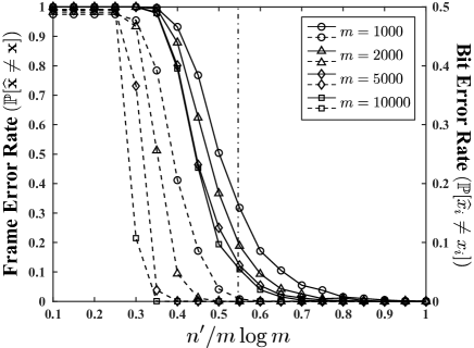
Figure 2: Frame error rate, $\mathbb{P}[{\widehat{\mathbf{x}}\neq\mathbf{x}}]$, (solid lines) and bit error rate $\mathbb{P}[\widehat{x}_{i}\neq x_{i}]$ (dashed lines) vs. (normalized) number of queries for four different values of $m$. Dash-dotted vertical lines are the information-theoretic limits for each $m$ given by Theorem 1.

We first show through simulation that Algorithm 1 achieves the bound established in Theorem 1 for finite $m$. We set $m$ to have values of 1000, 2000, 5000, and 10000, while fixing the number of workers to $w=100$. We vary the query degrees by letting them randomly sampled from $3$ to $6$ with equal probabilities, but we use a simple error model where the error probability does not depend on the query degree, as in the case of communication systems. Equal number of workers have the error probabilities, each from $\{0.02,0.04,\cdots,0.20\}$. Different from the original Algorithm 1 where each phase is conducted only once, to increase the accuracy of the estimates at a finite $m$, Phase 2 is iterated 10 times, and then Phases 3–4 are together iterated 10 times. Also, apart from the $m$ degree-1 queries used in Phase 1 of Algorithm 1, the queries are not divided into separates sets $A^{(2)}$, $A^{(3)}$, $A^{(4)}$, but all the queries are used together in both the iterations. In all the following experiments, we use this modified proposed algorithm. Denoting the number of queries used in the iterations as $n^{\prime}:=n-m$, we measured the frame error rate, $\operatorname*{\mathbb{P}}\left[\widehat{\mathbf{x}}\neq\mathbf{x}\right]$, and the average bit error rate, $\operatorname*{\mathbb{P}}\left[\widehat{x}_{i}\neq x_{i}\right]$, of the proposed algorithm with respect to $n^{\prime}$ by repeating the experiment 1000 times. The result is shown in Fig 2. The solid lines and dotted lines indicate frame and bit error rate, respectively, and the information-theoretic limit given by Theorem 1 is shown with the vertical dash-dotted line. We observe that the proposed computationally-efficient algorithm for XOR query nearly achieves the optimal sample complexity even when the noise parameters are unknown, and the algorithm converges faster at bigger $m$. The bit error rate drops at much smaller sample complexity than the limit, but it does not imply the perfect recovery.

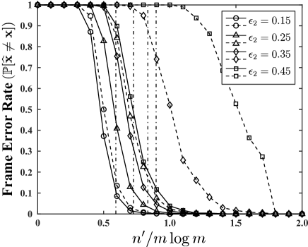
Figure 3: Frame error rate $\mathbb{P}[{\widehat{\mathbf{x}}\neq\mathbf{x}}]$ vs. (normalized) number of queries for four different combinations of worker reliabilities when the correct labels are inferred by Alg. 1 with (solid lines) and without (dashed lines) Phases 3–4. Dash-dotted vertical lines correspond to the information-theoretic limits of each case from $\epsilon_{2}=0.15$ (left most) to $\epsilon_{2}=0.45$ (right most).

In the next experiment, we compare the performances of Algorithm 1 with and without Phases 3–4, respectively, to validate the significance of estimating worker reliabilities. We consider a setting where the number of object labels $m=5000$ and the number of workers $w=100$. All queries have a fixed degree $d=4$ except the first $m$ degree-1 queries. The error probability of half of the workers is fixed to $\epsilon_{1}=0.05$, but that of the other half is varied to $\epsilon_{2}=0.15,0.25,0.35,0.45$. We assume that the degree-1 queries are assigned only to the first half of the workers. The error rates averaged over 1000 trials are summarized in Figure 3, where the solid lines correspond to the proposed algorithm and the dashed lines correspond to the proposed algorithm without Phases 3–4. As the variance of the workers’ reliability increases, i.e., for a higher $\epsilon_{2}$, the gap between the solid line and the dashed line increases. This shows that Phases 3–4 of the proposed algorithm, where worker reliabilities are estimated and used to refine the weakly recovered labels, become more important as the difference between workers’ reliabilities is greater.

V-B Comparison of Different Schemes with a Fair Error Model

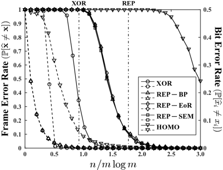
Figure 4: Frame error rate, $\mathbb{P}[{\widehat{\mathbf{x}}\neq\mathbf{x}}]$ (solid lines), and bit error rate $\mathbb{P}[\widehat{x}_{i}\neq x_{i}]$ (dashed lines) vs. (normalized) number of queries for five different pairs of query types and inference algorithms. Dash-dotted vertical lines are information-theoretic limits of XOR (left) and REP query (right).

In the first experiment, we assumed that the error probability of a worker remains constant regardless of query degree. However, we often encounter an application, e.g. crowdsourcing, such that the worker’s error probability depends on query degree, or in general, querying method. Hence, in order to fairly compare different querying methods and the inference algorithms, a proper error model is required that describes the change in worker’s error probability with respect to querying method. In this subsection, we propose such a noise model named $d$-coin flip model, and compare XOR queries with repetition (REP) and homogeneous (HOMO) queries.

In the $d$-coin flip model, given a query degree $d$, a worker $k$ independently flips $d$ coins, each of which gives head with probability $\epsilon_{k}$. When head has occurred, the worker makes wrong decision about the item corresponding to the coin, and after gathering $d$ decisions by the query operation, the final answer for the query is made. For example, the error probability of a degree-$d$ XOR query under the $d$-coin flip model becomes

$$\epsilon_{k,d}=\sum_{\begin{subarray}{c}l\in[1:d],\\ l\text{ odd}\end{subarray}}{d\choose l}\epsilon_{k}^{l}(1-\epsilon_{k})^{d-l}=\frac{1-(1-2\epsilon_{k})^{d}}{2}.$$ (8)

In this experiment, we chose the reliability parameter $\epsilon_{k}$ of each worker randomly from the set $\{0.010,0.020,\cdots,0.100\}$.

We use the number of object labels $m=5000$ and the number of workers $w=100$ as in the previous experiment. The query degrees of XOR query and HOMO query are uniformly sampled from 3 to 6, and the answers are collected with the $d$-coin flip noise model. As usual, the XOR query has additional $m$ degree-1 queries for the initialization, and the proposed algorithm is applied. For HOMO query, we apply the inference algorithm based on spectral clustering and local refinement, which has been shown to be order-wise optimal in [36]. For REP query, three state-of-the-art algorithms, based on belief propagation (BP) [3], spectral-EM (SEM) [8], and ratio of eigenvector (EoR) [7] are applied. Figure 4 shows the frame and bit error rates measured in 1000 trials versus (normalized) number of queries for the five different pairs of query types and inference algorithms. The $m$ degree-1 queries of XOR querying is also included in the plot. The result indicates the benefit of using XOR queries with high degrees over REP and HOMO queries in reducing the sample complexity for exact recovery. Although all the three algorithms for REP query nearly achieve the optimal sample complexity, the large gap between the fundamental limits of XOR query and that of repetition query (plotted by vertical lines) makes XOR query more efficient than REP query in terms of strong recovery. However, REP queries show better performance than XOR query in terms of bit error rate especially when the number of queries are small. The HOMO query turns out to be the worst among the three query types.

V-C Real Experiment: Crowdsourcing

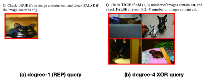
Figure 5: Examples of degree-1 and degree-4 queries.

Figure 6: Probability of error $\mathbb{P}[{\widehat{\mathbf{x}}\neq\mathbf{x}}]$ in strong recovery vs. number of queries for four different algorithms applied to real dataset from human workers.

In this subsection, we assess the practicality of XOR query and the proposed algorithm by applying them to a real crowdsourcing platform. We designed a binary classification task using 600 images of dogs and cats sampled from ImageNet [37], and collected data from the workers in Amazon Mechanical Turk. Each human intelligent task (HIT) was designed to include 20 degree-1 queries and 20 degree-4 XOR queries. The examples of each query type are shown in Figure 5. We designed 400 HITs and assigned each of them to 400 workers. The reward of each query was fixed to $0.01 regardless of the query degree. For the collected data, we compare how many queries $n$ are required to recover all the 600 labels when we use only degree-1 (REP) queries or we use 20 degree-4 XOR queries with additional 5 degree-1 queries from each HIT. For the REP queries we apply three different inference algorithms (BP, SEM, EoR) as in the previous experiment, and for the XOR queries we apply Algorithm 1. We repeat this experiment 10 times and plot the empirical error rate in Figure 6. The result shows that XOR query with the proposed algorithm outperforms REP query with BP or EoR algorithms, but it has similar performance to REP query with SEM algorithm. The theoretical limits (2) on the required number of queries calculated with the empirical noise parameters $\{\epsilon_{k,d}\}$ from the real dataset are 2300 for (degree-4) XOR query and 5200 for degree-1 REP query. In the experiment, the proposed algorithm with XOR query does not closely match this limit at the finite $m=600$, and thus the gain from the XOR query is not clearly seen. The reason could be that the number $m$ of images we use for the experiment is not large enough to meet the asymptotic information-theoretic limit.

VI Proof of Theorem 2: Analysis of Algorithm 2

In this section, we provide the proof of Theorem 2. The proof is separated into two parts: in the first part (Section VI-B), we will introduce a sequence of “good events” related to the query design and assignment that occurs with high probability; in the second part (Section VI-C), we will consider the answers we get from the queries and analyze the error probability of Algorithm 2 conditioned on the good events. In Section VI-A, we start by introducing a factor graph and the related definitions and notations that are required to define and analyze the good events and the performance of Algorithm 2

VI-A Factor Graph

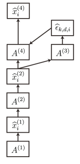
Figure 7: The dependency between the types of nodes.

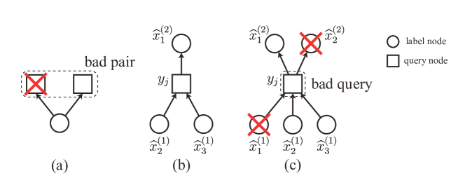
Figure 8: Factor graph for (a) bad pair (b) non-bad query (c) bad query. The figure is drawn assuming the degree of Phase 2 query $y_{j}$ is $3$ and $\partial y_{j}=\{1,2,3\}$.

When analyzing a message-passing type of algorithm, it is helpful to draw the factor graph, along the edges of which messages are transmitted. Thus, before we start proving Theorem 2, we introduce the symbolic meanings of the nodes in factor graph $G_{i}$ from the root $\widehat{x}_{i}^{(4)}$ of Algorithm 2.

First, we introduce three types of nodes present in the graph $G_{i}$: label node, query node, and worker node. Label nodes can be used to represent the three different estimates $\widehat{x}_{i^{\prime}}^{(1)}$, $\widehat{x}_{i^{\prime}}^{(2)}$, and $\widehat{x}_{i^{\prime}}^{(4)}$ that are made on label $x_{i^{\prime}}$ for $i^{\prime}\in[m]$ in Phase 1, 2, and 4 of Algorithm 2, respectively. Note that we depict the three estimates by different nodes although they have the same index $i^{\prime}$. There are four types of query nodes depending on in which phase of the algorithm (from Phase 1 to 4) the query is used. Each query node used in Phase 1, 2 and 4 outputs a message, $\operatorname{sgn}(y_{j})$, $m_{j\to i}^{(2)}$, $M_{j\to i}^{(4)}$, to each neighboring label node $i\in\partial y_{j}$, respectively, while each query node used in Phase 3 outputs a message $E_{j}^{(3)}$ to its neighboring worker node $w(j)$. Lastly, the worker node outputs a message $\widehat{\epsilon}_{k,d,i}$, which is the estimate on worker reliability made in Phase 3, to a Phase 4 query node.

An edge in factor graph represents the dependency between the nodes, or the direction to which the message is transmitted. We next figure out the dependency between the types of the nodes introduced above. The estimates on labels made in Phase 1, 2, and 4 are based on the messages from queries in the same phase. In order to calculate the messages, query nodes use the estimates on label nodes made in the previous phase, but as a special case, Phase 4 query nodes use the reliability estimates for worker nodes made in Phase 3 as well as the estimates on label nodes made in Phase 2 . To calculate the reliability estimates, worker nodes use the messages from Phase 3 query nodes. We summarize the dependency between the types of nodes in Figure 7, where the vertical position represents the level of nodes in the overall factor graph $G_{i}$. For example, Phase 2 label node is located in a higher level than Phase 2 query node, and Phase 3 and 4 query nodes are located in the same level.

We will explain two different cases where a cycle is created in the factor graph. The first case is when a label node is connected to two different query nodes in a higher level, as depicted in Figure 8-(a). We call the two query nodes a bad pair. When there exists a bad pair, we will delete one of the query nodes from the factor graph. The second case is when a query node sends messages (or connected) to more than one label nodes in a higher level. We call such a query a bad query. We define the badness of a bad query as the number of higher level nodes it is connected to, which is always larger than one by the definition. A non-bad query is depicted in Figure 8-(b) for comparison, with one higher-level label node and $d-1$ lower-level label nodes, where $d$ is the query degree. A bad query with badness equal to two is depicted in Figure 8-(c). Unlike a non-bad query, a bad query is always connected to $d$ lower-level label nodes since all the estimates on the $d$ labels are required to calculate the messages to any two or more different higher-level label nodes. If there exists a bad query, we delete $(\textit{badness}-1)$ number of higher-level nodes so as to make only one node left in the higher level, and also delete the lower-level node that has the same index with the remaining higher-level node since it is not required anymore.

In the next subsection, we will define “good events” on the factor graph $G_{i}$ such that there are only a few bad pairs and a few bad queries so that by removing a few nodes we can make $G_{i}$ a tree with high probability.

VI-B Good Events

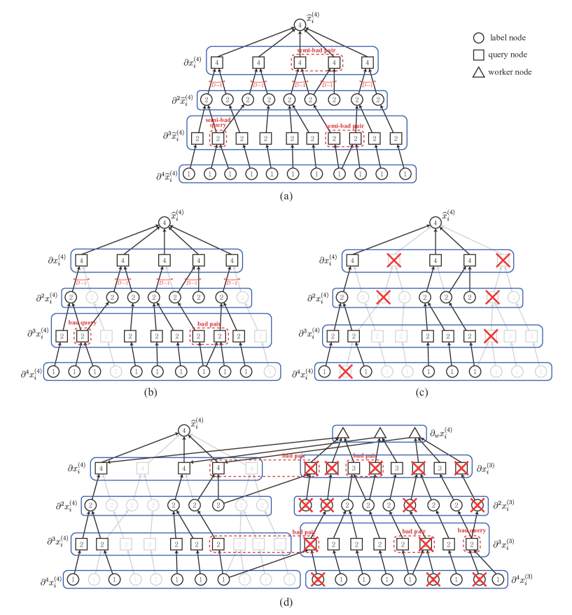
Figure 9: The numbers in nodes indicate the phase of Algorithm 2 to which each node belongs. (a) An example of the factor graph generated after step 4). (b) The factor graph after obtaining the true degree of each query in $\partial x_{i}^{(4)}$ and selecting $\partial y_{j}\setminus\{i\}$ from $\partial\widetilde{y}_{j}$. (c) The factor graph after the removal of bad queries and bad pairs in step 5). (d) The final factor graph with an illustration of the bad pairs and bad queries made in steps 6) – 10).

We explain the detailed sequential process of drawing $G_{i}$ in this subsection. We will also introduce “good events” related to each step of the process. The good events we define occur with probability exceeding $1-o(1/m)$ so that it does not affect the error analysis. Basically, there are two types of good events regarding the random graph $G_{i}$. The events of the first type assert that there are not many bad pairs and bad queries in $G_{i}$ and by removing a few query nodes from $G_{i}$ we can make the remaining graph a tree with high probability. The second type is related to the number of queries connected to $\widehat{x}_{i}^{(4)}$ and to $\widehat{\epsilon}_{k,d,i}$ that are helpful in correctly estimating the label $x_{i}$ and the noise parameters $\{\epsilon_{k,d}\}$, respectively.

We explain the first type of good events related to independence of messages used for the estimation of $x_{i}$ and $\{\epsilon_{k,d}\}$, by considering the random process of generating a factor graph $G_{i}$ from the root $\widehat{x}_{i}^{(4)}$ according to the random query design and assignment model, explained in Section II-A. The process of generating $G_{i}$ and how the bad pairs and bad queries appear in the graph are depicted in Fig. 9.

1. At the first step, a subset of Phase 4 queries are connected to $x_{i}$ according to the random query design model, where each query in $A^{(4)}$ is connected to $x_{i}$ with probability $\overline{d}/m$, independently, where $\overline{d}=\sum_{d=1}^{D}d\Phi_{d}$ is the average query degree. We denote the set of Phase 4 queries connected to $x_{i}$ as

   $$\partial x_{i}^{(4)}:=\partial x_{i}\cap A^{(4)}.$$ (9)

2. Next, each query node $y_{j}$ for $j\in\partial x_{i}^{(4)}$ needs to select $d-1$ label nodes from $[m]\backslash\{i\}$ uniformly at random. The query degree $d$ of each query is sampled from the distribution $\left\{\frac{d\Phi_{d}}{\overline{d}}\right\}$ instead of $\{\Phi_{d}\}$, since conditioned on that $y_{j}$ is already connected to $x_{i}$ the degree distribution of each query increases proportional to $d$. We divide this label-selection process for $y_{j}$ into the following three steps: (a) each query node $y_{j}$ first selects $D-1$ label nodes randomly from $[m]\backslash\{i\}$, and we denote this set of label nodes by $\partial\widetilde{y}_{j}$, (b) the true degree $d$ is sampled from the distribution $\left\{\frac{d\Phi_{d}}{\overline{d}}\right\}$, and (c) $d-1$ label nodes are randomly sampled from $\partial\widetilde{y}_{j}$ to construct $\partial y_{j}\setminus\{i\}$. We assume that only step (a) is performed here, and steps (b) and (c) are postponed until step 5).

   The reason we introduced the set $\partial\widetilde{y}_{j}$ is to acquire symmetry between the queries in $\partial x_{i}^{(4)}$ regardless of the true degree $d$. We also note that $\partial\widetilde{y}_{j}$ is a kind of latent variable that is not revealed to Algorithm 2, and some of the nodes in $\partial\widetilde{y}_{j}$ may not be contained in $G_{i}$. Thus, $\partial\widetilde{y}_{j}$ will be used not for the operations of Algorithm 2, but only for the purpose of proving the performance of the algorithm later.

   The set of label nodes selected in this step is denoted by

   $$\partial^{2}\widetilde{x}_{i}^{(4)}:=\bigcup_{j\in\partial x_{i}^{(4)}}\partial\widetilde{y}_{j}.$$ (10)

   In this step, if a pair of queries $(j_{1},j_{2})$ in $\partial x_{i}^{(4)}$ selects the same label from $[m]\backslash\{i\}$, i.e. $\partial\widetilde{y}_{j_{1}}\cap\partial\widetilde{y}_{j_{2}}\neq\varnothing$, we call this pair a semi-bad pair. We call it a semi-bad pair, since it may or may not be a bad pair after we choose the actual $\partial y_{j_{1}}(\subset\partial\widetilde{y}_{j_{1}})$ and $\partial y_{j_{2}}(\subset\partial\widetilde{y}_{j_{2}})$. Also, note that a bad pair is always a semi-bad pair. We will later show that there is at most one semi-bad pair in $\partial x_{i}^{(4)}$, thus at most one bad pair in $\partial x_{i}^{(4)}$.

3. At the third step, we start considering Phase 2 query assignment, and specify the set of queries connected to each label node in $\partial^{2}\widetilde{x}_{i}^{(4)}$. First, the degree of each query in Phase 2 query set $A^{(2)}$ is sampled from $\{\Phi_{d}\}$. We then separate the queries in $A^{(2)}$ into two sets depending on whether a query selects at least one label node in $\partial^{2}\widetilde{x}_{i}^{(4)}$ or not. Denote by $\partial^{3}\widetilde{x}_{i}^{(4)}$ the set of queries in $A^{(2)}$ that select at least one label node in $\partial^{2}\widetilde{x}_{i}^{(4)}$

   $$\partial^{3}\widetilde{x}_{i}^{(4)}:=\left\{\bigcup_{i^{\prime}\in\partial^{2}\widetilde{x}_{i}^{(4)}}\partial x_{i^{\prime}}\right\}\bigcap A^{(2)}.$$ (11)

   Each query of degree-$d$ in $A^{(2)}$ is included in the set $\partial^{3}\widetilde{x}_{i}^{(4)}$ independently with probability $1-\frac{{m-|\partial^{2}\widetilde{x}_{i}^{(4)}|\choose d}}{{m\choose d}}$.

4. At the next step, each query in $\partial^{3}\widetilde{x}_{i}^{(4)}$ selects its labels conditioned on that it should select at least one label from $\partial^{2}\widetilde{x}_{i}^{(4)}$. Hence, we first let each degree-$d$ query in $\partial^{3}\widetilde{x}_{i}^{(4)}$ randomly select one label from $\partial^{2}\widetilde{x}_{i}^{(4)}$, and then let them select the remaining $d-1$ labels uniformly at random from the remaining $m-1$ labels in $[m]$. If a query selects more than one label from $\partial^{2}\widetilde{x}_{i}^{(4)}$, we call such a query a semi-bad query. The badness of a semi-bad query is defined the same as that of a bad query. Also, if a pair of queries selects the same label not in $\partial^{2}\widetilde{x}_{i}^{(4)}$, the pair is called a semi-bad pair as before. We will show that there are at most one semi-bad query with badness equal to two, and at most one semi-bad pair in $\partial^{3}\widetilde{x}_{i}^{(4)}$. We will also show that there is no semi-bad query with badness larger than two. Let us define $\partial^{4}\widetilde{x}_{i}^{(4)}$ as the index set of Phase 1 label nodes connected to Phase 2 query nodes in $\partial^{3}\widetilde{x}_{i}^{(4)}$. When there is no semi-bad query, it is equal to

   $$\partial^{4}\widetilde{x}_{i}^{(4)}=\left\{\bigcup_{j\in\partial^{3}\widetilde{x}_{i}^{(4)}}\partial y_{j}\right\}\setminus\partial^{2}\widetilde{x}_{i}^{(4)},$$ (12)

   but when there is a semi-bad query, $\partial^{4}\widetilde{x}_{i}^{(4)}$ may include some labels in $\partial^{2}\widetilde{x}_{i}^{(4)}$. The factor graph constructed up to this point is depicted in Figure 9-(a).

5. Now, we perform the steps (b) and (c) of the label-selection process for queries in $\partial x_{i}^{(4)}$ as introduced in step 2). After this, we will be given the set of label nodes in $\partial^{2}\widetilde{x}_{i}^{(4)}$ that are actually connected to the queries in $\partial x_{i}^{(4)}$ in $G_{i}$. We denote the set by

   $$\partial^{2}x_{i}^{(4)}:=\bigcup_{j\in\partial x_{i}^{(4)}}\partial y_{j}\setminus\{i\}.$$ (13)

   We remove from the factor graph the child nodes of $\partial^{2}\widetilde{x}_{i}^{(4)}$ that is not connected to $\partial^{2}x_{i}^{(4)}$, and define the survived nodes in $\partial^{3}\widetilde{x}_{i}^{(4)}$ and $\partial^{4}\widetilde{x}_{i}^{(4)}$ as $\partial^{3}x_{i}^{(4)}$ and $\partial^{4}x_{i}^{(4)}$, respectively. The resulting factor graph after this step is depicted in Figure 9-(b). We check whether the semi-bad queries and semi-bad pairs are still present in the factor graph, and if so, since they are bad queries or bad pairs, we remove some of the queries in $\partial x_{i}^{(4)}$ and the child nodes of them to eliminate the bad queries and bad pairs. There are at most one bad pair in $\partial x_{i}^{(4)}$, one bad pair and one bad query with badness equal to two in $\partial^{3}x_{i}^{(4)}$, and thus by removing at most three queries from $\partial x_{i}^{(4)}$ we can make the remaining graph a tree. An example of this process is depicted in Figure 9-(c). After the removal of the nodes, the definition of the sets $\partial x_{i}^{(4)},\partial^{2}x_{i}^{(4)},\partial^{3}x_{i}^{(4)},\partial^{4}x_{i}^{(4)}$ are updated to include only the survived nodes at each level of the factor graph.

6. The remaining steps are related to the estimation of workers’ reliabilities $\{\epsilon_{k,d}\}$. We first specify the set of workers who answer for each query in $\partial x_{i}^{(4)}$. Remind that each query is assigned to a worker randomly selected from $[w]$. Let us define the set of $(k,d)$ for which the worker $k\in[w]$ is assigned to at least one degree-$d$ query in $\partial x_{i}^{(4)}$, i.e.,

   $$\begin{split}\partial_{w}x_{i}^{(4)}=&\{(k,d)\in[W]\times[D]:w(j)=k,\;\;d(j)=d\text{ for some }j\in\partial x_{i}^{(4)}\}.\end{split}$$ (14)

   We can also interpret $\partial_{w}x_{i}^{(4)}$ as the set of worker nodes connected to $\partial x_{i}^{(4)}$.

7. The next step is to assign Phase 3 queries to the worker nodes in $\partial_{w}x_{i}^{(4)}$. Let us define $\partial x_{i}^{(3)}$ as the set of queries in $A^{(3)}$ assigned to any worker in $\partial_{w}x_{i}^{(4)}$, i.e.

   $$\partial x_{i}^{(3)}=\bigcup_{(k,d)\in\partial_{w}x_{i}^{(4)}}\partial w_{k,d}^{(3)},$$ (15)

   where $\partial w_{k,d}^{(3)}=\partial w_{k}\bigcap A_{d}^{(3)}$ is the set of Phase 3 queries assigned to the worker node $(k,d)\in\partial_{w}x_{i}^{(4)}$.

8. Next, each query in $\partial x_{i}^{(3)}$ selects $d$ labels from $[m]$ uniformly at random, where $d$ is sampled from the degree distribution $\{\Phi_{d}\}$. Let us define the set of label nodes selected by $\partial x_{i}^{(3)}$ as

   $$\partial^{2}x_{i}^{(3)}:=\MT@delim@PAIRED\set@star{\bigcup_{j\in\partial x_{i}^{(3)}}\partial y_{j}}.$$ (16)

   We will prove that at most one query in $\partial x_{i}^{(3)}$ selects a label in $\partial^{2}\widetilde{x}_{i}^{(4)}\cup\partial^{4}\widetilde{x}_{i}^{(4)}$. This good event implies that we should delete at most one query in $\partial x_{i}^{(3)}$ to remove any bad pair or bad query made by the following three cases. First, if any query in $\partial x_{i}^{(3)}$ selects a label in $\partial^{2}x_{i}^{(4)}$, the query forms a bad pair with a query in $\partial x_{i}^{(4)}$. We remove all such bad pairs by removing the corresponding query in $\partial x_{i}^{(3)}$ and thus make $\partial^{2}x_{i}^{(4)}\cap\partial^{2}x_{i}^{(3)}=\varnothing$. Second, if any query in $\partial x_{i}^{(3)}$ selects a label in $\partial^{4}x_{i}^{(4)}$, a bad query is created in $\partial^{3}x_{i}^{(4)}$ that selects a label from both $\partial^{2}x_{i}^{(4)}$ and $\partial^{2}x_{i}^{(3)}$. Third, if any query in $\partial x_{i}^{(3)}$ selects a label in $\partial^{2}\widetilde{x}_{i}^{(4)}\setminus\partial^{2}x_{i}^{(4)}$ or in $\partial^{4}\widetilde{x}_{i}^{(4)}\setminus\partial^{4}x_{i}^{(4)}$ that is connected to a semi-bad pair or a semi-bad query in $\partial^{3}\widetilde{x}_{i}^{(4)}$, the semi-bad pair or the semi-bad query can turn back to a bad pair or a bad query in $G_{i}$. For both the second and third case, we remove the corresponding query in $\partial x_{i}^{(3)}$. Note that in these cases, it suffices to remove only one query in $\partial x_{i}^{(3)}$ regardless of the badness of the bad query. We can then guarantee that there is no Phase 2 query that selects a label from both $\partial^{2}x_{i}^{(4)}$ and $\partial^{2}x_{i}^{(3)}$, since no Phase 2 query other than $\partial^{3}\widetilde{x}_{i}^{(4)}$ can select a label from $\partial^{2}x_{i}^{(4)}$. We also prove that there is at most one bad pair in $\partial x_{i}^{(3)}$ with probability $1-o(1/m)$. Hence, in total we remove at most $2$ query nodes from $\partial x_{i}^{(3)}$ in this step.

9. In this step, we assign Phase 2 queries to $\partial^{2}x_{i}^{(3)}$. Since we have already finished assignment of the queries in $\partial^{3}\widetilde{x}_{i}^{(4)}$ in step 4), here we consider only the queries in $A^{(2)}\setminus\partial^{3}\widetilde{x}_{i}^{(4)}$. Again, we separate the queries in $A^{(2)}\setminus\partial^{3}\widetilde{x}_{i}^{(4)}$ into two sets depending on whether a query selects at least one label node in $\partial^{2}x_{i}^{(3)}$ or not, and define $\partial^{3}\widetilde{x}_{i}^{(3)}$ to be the set of queries in $A^{(2)}\backslash\partial^{3}\widetilde{x}_{i}^{(4)}$ that select at least one label node in $\partial^{2}x_{i}^{(3)}$, i.e.,

   $$\partial^{3}\widetilde{x}_{i}^{(3)}:=\left\{\bigcup_{i^{\prime}\in\partial^{2}x_{i}^{(3)}}\partial x_{i^{\prime}}\right\}\bigcap\left\{A^{(2)}\backslash\partial^{3}\widetilde{x}_{i}^{(4)}\right\}.$$ (17)

   If there exists a label in $\partial^{2}x_{i}^{(3)}$ that also belongs to $\partial^{2}\widetilde{x}_{i}^{(4)}$ or $\partial^{4}\widetilde{x}_{i}^{(4)}$ (there is at most one such label as stated in step 8)), this label is connected to some query in $\partial^{3}\widetilde{x}_{i}^{(4)}$. Thus, some of the Phase 2 queries that are connected to $\partial^{2}x_{i}^{(3)}$ may not be contained in $\partial^{3}\widetilde{x}_{i}^{(3)}$, and we define

   $$\partial^{3}x_{i}^{(3)}:=\left\{\bigcup_{i^{\prime}\in\partial^{2}x_{i}^{(3)}}\partial x_{i^{\prime}}\right\}\bigcap A^{(2)}$$ (18)

   as the set of Phase 2 queries that select at least one label node in $\partial^{2}x_{i}^{(3)}$. Note that the query-to-label assignment for the queries in $\partial^{3}x_{i}^{(3)}\setminus\partial^{3}\widetilde{x}_{i}^{(3)}$ has already done in step 4).

10. We then make each query in $\partial^{3}\widetilde{x}_{i}^{(3)}$ select one label randomly from $\partial^{2}x_{i}^{(3)}\setminus\partial^{2}\widetilde{x}_{i}^{(4)}$. We have to exclude the labels in $\partial^{2}\widetilde{x}_{i}^{(4)}$, since any query that selects $\partial^{2}\widetilde{x}_{i}^{(4)}$ is already in $\partial^{3}\widetilde{x}_{i}^{(4)}$ and $\partial^{3}\widetilde{x}_{i}^{(3)}\cap\partial^{3}\widetilde{x}_{i}^{(4)}=\varnothing$ by definition. Lastly, each query in $\partial^{3}\widetilde{x}_{i}^{(3)}$ with degree $d$ selects the $d-1$ labels uniformly at random from the remaining nodes in $[m]$ except $\partial^{2}\widetilde{x}_{i}^{(4)}$. At most one query in $\partial^{3}\widetilde{x}_{i}^{(3)}$ selects a label in $\partial^{4}\widetilde{x}_{i}^{(4)}\setminus\partial^{2}x_{i}^{(3)}$ (the set difference accounts for the case where there is a label in $\partial^{2}x_{i}^{(3)}$ that also belongs to $\partial^{4}\widetilde{x}_{i}^{(4)}$), and by removing the corresponding query in $\partial x_{i}^{(3)}$ if necessary, we can exclude the cases where a query in $\partial^{3}\widetilde{x}_{i}^{(3)}$ forms a bad pair with a query in $\partial^{3}x_{i}^{(4)}$ or with a query in $\partial^{3}x_{i}^{(3)}\setminus\partial^{3}\widetilde{x}_{i}^{(3)}$. We also prove that there is at most one bad pair and at most one bad query with badness equal to two in $\partial^{3}\widetilde{x}_{i}^{(3)}$, and there is no bad query with badness larger than two. Thus, in this step, we remove at most three queries in $\partial x_{i}^{(3)}$, and in total at most five queries are removed from $\partial x_{i}^{(3)}$ to remove all the cycles. Figure 9-(d) shows an example of the inference graph and the nodes to be eliminated to remove the loops.

Algorithm 3 Phase 0 of Algorithm 2

1:  If there is a bad pair such that both of the queries are in $\partial x_{i}^{(4)}$, remove one of the query in the bad pair.

2:  If there is a bad query in $\partial^{3}x_{i}^{(4)}$ that is connected to two label nodes in $\partial^{2}x_{i}^{(4)}$, remove a node in $\partial x_{i}^{(4)}$ that is the parent of one of the two nodes. If there is a bad query in $\partial^{3}x_{i}^{(4)}$ with badness larger than two, claim an error.

3:  If there is a bad pair such that both of the queries are in $\partial^{3}x_{i}^{(4)}$, remove a node in $\partial x_{i}^{(4)}$ that is the parent of one of the two query nodes.

4:  If there is a bad pair such that one query is in $\partial x_{i}^{(4)}$ and the other is in $\partial x_{i}^{(3)}$, remove the query in $\partial x_{i}^{(3)}$ in the bad pair.

5:  If there is a bad query in $\partial^{3}x_{i}^{(4)}$ that is connected to two label nodes each in $\partial^{2}x_{i}^{(4)}$ and $\partial^{2}x_{i}^{(3)}$, remove the node in $\partial x_{i}^{(3)}$ that is the parent of the node in $\partial^{2}x_{i}^{(3)}$.

6:  If there is a bad pair such that both of the queries are in $\partial x_{i}^{(3)}$, remove one of the query in the bad pair.

7:  If there is a bad pair such that one query is in $\partial^{3}x_{i}^{(4)}$ and the other is in $\partial^{3}x_{i}^{(3)}$, remove a node in $\partial x_{i}^{(3)}$ that is the parent of the query node in $\partial^{3}x_{i}^{(3)}$.

8:  If there is a bad query in $\partial^{3}x_{i}^{(3)}$ that is connected to two label nodes in $\partial^{2}x_{i}^{(3)}$, remove a node in $\partial x_{i}^{(3)}$ that is the parent of one of the two nodes. If there is a bad query in $\partial^{3}x_{i}^{(3)}$ with badness larger than two, claim an error.

9:  If there is a bad pair such that both of the queries are in $\partial^{3}x_{i}^{(3)}$, remove the query in $\partial x_{i}^{(3)}$ that is the parent of one of the two query nodes.

10:  Claim an error if we have to remove more than three queries in $\partial x_{i}^{(4)}$ or more than five queries in $\partial x_{i}^{(3)}$ from the above steps.

With the discussions made above, we can now state Phase 0 of the Algorithm 2 in an explicit way as in Algorithm 3. The first three steps of Algorithm 3 are related to step 5), the fourth to the sixth steps are related to step 8), and the seventh to the ninth steps are related to step 10). We claim that Algorithm 3 succeeds with probability $1-o(1/m)$.

Lemma 1.

By removing at most three queries in $\partial x_{i}^{(4)}$ and at most five queries in $\partial x_{i}^{(3)}$ as described in Algorithm 3, all the bad pairs and the bad queries in $G_{i}$ are removed with probability $1-o(1/m)$, and $G_{i}$ becomes a tree.

Proof:

The proof of this lemma is provided in Appendix B. ∎

The tree structure of $G_{i}$ implies the following four independence results (or good events) that we will use in the analysis of error probability.

1. For each $i^{\prime}\in\partial^{2}x_{i}^{(4)}\cup\partial^{2}x_{i}^{(3)}$, the messages $\{m^{(2)}_{j\to i^{\prime}}\}_{j\in\partial x_{i^{\prime}}\cap A^{(2)}}$, which are used to generate $\widehat{x}_{i^{\prime}}^{(2)}$, are independent.

2. The estimators $\{\widehat{x}_{i^{\prime}}^{(2)}\}_{i^{\prime}\in\partial^{2}x_{i}^{(3)}\cup\partial^{2}x_{i}^{(4)}}$ are independent.

3. For each $(k,d)\in\partial_{w}x_{i}^{(4)}$, the messages $\{E_{j}^{(3)}\}_{j\in\partial w_{k,d}^{(3)}}$, which are used to generate $\widehat{\epsilon}_{k,d,i}$, are independent.

4. The messages $\{m_{j\to i}^{(4)}\}_{j\in\partial x_{i}^{(4)}}$ and the estimators $\{\widehat{\epsilon}_{k,d,i}\}_{(k,d)\in\partial_{w}x_{i}^{(4)}}$, which are used to generate the final estimate $\widehat{x}_{i}^{(4)}$, are all independent.

We move on to the second type of good events that are required to generate accurate estimates $\{\widehat{x}_{i}^{(2)}\}$, $\{\widehat{\epsilon}_{k,d,i}\}$ and $\widehat{x}_{i}^{(4)}$. We focus on controlling the number of three types of nodes, defined as good labels, perfect queries, and good queries.

Definition 1.

A label node $i^{\prime}\in\partial^{2}\widetilde{x}_{i}^{(4)}\bigcup\partial^{2}x_{i}^{(3)}$ is called a good label if $|\partial x_{i^{\prime}}\cap A^{(2)}|$, the number of queries in $A^{(2)}$ that have selected $x_{i^{\prime}}$, is $\Theta\left(\frac{\log m}{\log\log m}\right)$. We call a query $j\in\partial x_{i}^{(4)}$ a perfect query if all the $D-1$ label nodes in $\partial\widetilde{y}_{j}$ (before selecting the actual $d-1$ neighboring label nodes $\partial y_{j}\backslash\{i\}$ from $\partial\widetilde{y}_{j}$) are good labels and it is not a parent node of any semi-bad pair or semi-bad query. We also call a query $j\in\partial x_{i}^{(3)}$ a good query if all the $d$-neighboring label nodes $\partial y_{j}$ are good labels.

The set of good events for the accuracy of the estimator $\widehat{x}_{i}^{(4)}$ is as below.

1. The number of Phase 4 queries $A^{(4)}$ connected to $x_{i}$ is $|\partial x_{i}^{(4)}|=\Theta(\log m)$, and the number of perfect queries among $\partial x_{i}^{(4)}$ is at least $|\partial x_{i}^{(4)}|-C_{11}\log\log m-3$ for some constant $C_{11}>0$.

2. For each worker $(k,d)\in\partial_{w}x_{i}^{(4)}$, the number of Phase 3 queries assigned to $(k,d)$ is $|\partial w_{k,d}^{(3)}|=\Theta((\log m)(\log\log m))$, and there are at least $|\partial w_{k,d}^{(3)}|-C_{12}\log\log m-6$ good queries in $\partial w_{k,d}^{(3)}$ for some constant $C_{12}>0$.

Note that the average numbers of $|\partial x_{i}^{(4)}|$ and $|\partial w_{k,d}^{(3)}|$ are $\Theta(\log m)$ and $\Theta((\log m)(\log\log m))$, respectively, and under good events (v) and (vi) almost all the queries in $|\partial x_{i}^{(4)}|$ and $|\partial w_{k,d}^{(3)}|$ are perfect/good queries, respectively. We now claim that the intersection of the above two good events also holds with high probability.

Lemma 2.

The intersection of good events (v)–(vi) holds with probability $1-o(1/m)$.

Proof:

The proof of this lemma is provided in Appendix C. ∎

VI-C Proof of Theorem 2: Error Analysis under Good Events

We prove Theorem 2 conditioned on the intersection of good events (i)–(vi) defined in the previous section, which occurs with probability $1-o(1/m)$ by Lemma 1 and 2. Therefore, once we prove $\operatorname*{\mathbb{P}}\left[\widehat{x}_{i}^{(4)}\neq x_{i}\big{|}\text{good events}\right]=o(1/m)$ for all $i\in[m]$, then it implies $\operatorname*{\mathbb{P}}\left[\widehat{x}_{i}^{(4)}\neq x_{i}\right]=o(1/m)$ for all $i\in[m]$ and $\operatorname*{\mathbb{P}}\left[{\widehat{\mathbf{x}}^{(4)}}\neq\mathbf{x}\right]\to 0$ as $m\to\infty$ by union bound.

To prove Theorem 2, we first state Lemma 3–5, each of which describes the accuracy of the estimates $\{\widehat{x}_{i^{\prime\prime}}^{(1)}\},\{\widehat{x}_{i^{\prime}}^{(2)}\},\{\widehat{\epsilon}_{k,d,i}\}$, respectively, after Phase 1–3 of Algorithm 2, respectively. In proving lemmas, we assume that we have removed at most three queries in $\partial x_{i}^{(4)}$ and at most five queries in $\partial x_{i}^{(3)}$ and obtained the independence as stated in Lemma 1.

Lemma 3.

After Phase 1 of Algorithm 2, where we use total $n^{(1)}=m$ number of degree-1 queries to have an initial estimate on the labels, the detection of the labels $\{x_{i^{\prime\prime}}\}$ is guaranteed with $\{\widehat{x}_{i^{\prime\prime}}^{(1)}\}$ in (4), i.e.,

$$p^{(1)}:=\operatorname*{\mathbb{P}}\left[\widehat{x}_{i^{\prime\prime}}^{(1)}\neq x_{i^{\prime\prime}}\right]<1/2,\quad\forall i^{\prime\prime}\in\partial^{4}\widetilde{x}_{i}^{(4)}\cup\partial^{4}x_{i}^{(3)}.$$ (19)

We dropped the subscript $i^{\prime\prime}$ in $p^{(1)}$ since every label node is queried exactly once by the first $m$ degree-1 queries and thus the accuracy of the estimates is the same for all $i^{\prime\prime}\in\partial^{4}\widetilde{x}_{i}^{(4)}\cup\partial^{4}x_{i}^{(3)}$. Since every answer is better than a random guess by the assumption that $\epsilon_{k,1}<1/2$ for all $k\in[w]$, this lemma is obvious.

Lemma 4.

After Phase 2 of Algorithm 2 where we use total $n^{(2)}=m\left(\frac{\log m}{\log\log m}\right)$ number of queries to generate the second estimates on labels, the weak recovery of the labels $\{x_{i^{\prime}}\}$ is guaranteed with $\{\widehat{x}_{i^{\prime}}^{(2)}\}$ in (5) for good labels $i^{\prime}\in\partial^{2}\widetilde{x}_{i}^{(4)}\bigcup\partial^{2}x_{i}^{(3)}$ such that $|\partial x_{i^{\prime}}\cap A^{(2)}|=\Theta\left(\frac{\log m}{\log\log m}\right)$; for some $p^{(2)}=o(1/\log m)$,

$$\operatorname*{\mathbb{P}}\left[\widehat{x}_{i}^{(2)}\neq x_{i}\right]\leq p^{(2)}=o(1/\log m)$$ (20)

for all the good labels $i^{\prime}\in\partial^{2}\widetilde{x}_{i}^{(4)}\bigcup\partial^{2}x_{i}^{(3)}$.

Lemma 5.

After Phase 3 of Algorithm 2 where we use $n^{(3)}=w(\log m)(\log\log m)$ number of queries to estimate reliability of workers, conditioned on good events (v)–(vi), for every $(k,d)\in\partial_{w}x_{i}^{(4)}$ the estimate $\widehat{\epsilon}_{k,d,i}$ of the reliability of the $k$-th worker for the degree-$d$ query used for the estimation of $x_{i}$ satisfies

$$|\widehat{\epsilon}_{k,d,i}-\epsilon_{k,d}|=O(1/(\log\log m)^{1/4})$$ (21)

with probability at least $1-o(1/m)$, when the number of workers $w=o(m/\log\log m)$.

The proofs of Lemmas 4–5 are provided at the end of this section.

Finally, we are ready to bound the error probability $\operatorname*{\mathbb{P}}\left[\widehat{x}_{i}^{(4)}\neq x_{i}\right]$. We start from not conditioning any good events. By conditioning the number $a=|\partial x_{i}^{(4)}|$ of queries in $A^{(4)}$ connected to $x_{i}$, the error probability can be written as

$$\begin{split}\operatorname*{\mathbb{P}}\left[\widehat{x}_{i}^{(4)}\neq x_{i}\right]&=\sum_{a\in[n^{(4)}]}\operatorname*{\mathbb{P}}\left[|\partial x_{i}^{(4)}|=a\right]\operatorname*{\mathbb{P}}\left[\widehat{x}_{i}^{(4)}\neq x_{i}\Big{|}|\partial x_{i}^{(4)}|=a\right]\\ &=\sum_{a\in[n^{(4)}]}{n^{(4)}\choose a}\left(\frac{\overline{d}}{m}\right)^{a}\left(1-\frac{\overline{d}}{m}\right)^{n^{(4)}-a}\operatorname*{\mathbb{P}}\left[\widehat{x}_{i}^{(4)}\neq x_{i}\Big{|}|\partial x_{i}^{(4)}|=a\right],\end{split}$$ (22)

since each query in $A^{(4)}$ is connected to $x_{i}$ independently with probability $\overline{d}/m$. We first show that $|\partial x_{i}^{(4)}|$ is $\Theta(\log m)$ with probability $1-o(1/m)$. Since the total number of $A^{(4)}$ queries is $\Theta(m\log m)$ and the number of labels is $m$, the average number of queries connected to each label is $\Theta(\log m)$.

Lemma 6.

Let us define the event $S_{1}$ as

$S_{1}$: $c_{1}\log m<|\partial x_{i}^{(4)}|<C_{1}\log m$

for some constants $C_{1}>c_{1}>0$. Then, we have $\operatorname*{\mathbb{P}}\left[S_{1}\right]\geq 1-o(1/m)$.

Note that the event $S_{1}$ is a part of the good event (v), which will be proved in Appendix B. By Lemma 6, we have

$$\begin{split}\operatorname*{\mathbb{P}}\left[\widehat{x}_{i}^{(4)}\neq x_{i}\right]&\leq\sum_{a\in S_{1}}{n^{(4)}\choose a}\left(\frac{\overline{d}}{m}\right)^{a}\left(1-\frac{\overline{d}}{m}\right)^{n^{(4)}-a}\operatorname*{\mathbb{P}}\left[\widehat{x}_{i}^{(4)}\neq x_{i}\Big{|}|\partial x_{i}^{(4)}|=a\right]+o(1/m).\end{split}$$ (23)

Next, we analyze $\operatorname*{\mathbb{P}}\left[\widehat{x}_{i}^{(4)}\neq x_{i}\Big{|}|\partial x_{i}^{(4)}|=a\right]$ for $a\in S_{1}$. From this point, the error analysis is conditioned on the intersection of the good events (i)–(vi), which hold with probability $1-o(1/m)$ by Lemma 1 and 2. Remind that Phase 4 estimate of $x_{i}$ is defined as $\widehat{x}_{i}^{(4)}=\operatorname{sgn}\Bigg{(}\sum_{j\in\partial x_{i}^{(4)}}M_{j\to i}^{(4)}\Bigg{)}$, where $M_{j\to i}^{(4)}=\log\bigg{(}\frac{1-\widehat{\epsilon}_{w(j),d(j),i}}{\widehat{\epsilon}_{w(j),d(j),i}}\bigg{)}m_{j\to i}^{(4)}.$ Conditioned on the sequence of good events, by Lemma 5 we can have the estimates on worker reliabilities $\{\widehat{\epsilon}_{k,d,i}\}$ satisfying $|\widehat{\epsilon}_{k,d,i}-\epsilon_{k,d}|=O(1/(\log\log m)^{1/4})$ for every $(k,d)\in\partial_{w}x_{i}^{(4)}$, with probability $1-o(1/m)$. Let us define this event as

$$\begin{split}\mathcal{E}:=\{&{|\widehat{\epsilon}_{k,d,i}-\epsilon_{k,d}|=O(1/(\log\log m)^{1/4})}\text{ for every }(k,d)\in\partial_{w}x_{i}^{(4)}\}.\end{split}$$ (24)

So, by conditioning on the event $\mathcal{E}$ and by using the independence of the messages $\{M_{j\to i}\}_{i\in\partial j\in\partial x_{i}^{(4)}}$ implied by the good event (iv), we get

$$\begin{split}\operatorname*{\mathbb{P}}\left[\widehat{x}_{i}^{(4)}\neq x_{i}\Big{|}|\partial x_{i}^{(4)}|=a\right]&=\operatorname*{\mathbb{P}}\left[\sum_{j\in\partial{x}_{i}^{(4)}}-x_{i}M_{j\to i}^{(4)}\geq 0\right]\\ &=\prod_{(k,d)\in\partial_{w}x_{i}^{(4)}}\prod_{\{j\in\partial{x}_{i}^{(4)}:w(j)=k,d(j)=d\}}\operatorname*{\mathbb{E}}\left[e^{-tx_{i}M_{j\to i}^{(4)}}\Bigg{|}\mathcal{E}\right]+o(1/m).\end{split}$$ (25)

for some $t>0$.

We next analyze $\operatorname*{\mathbb{E}}\left[e^{-tx_{i}M_{j\to i}^{(4)}}\Bigg{|}\mathcal{E}\right]$, depending on whether $j\in\partial{x}_{i}^{(4)}$ is a perfect query or not. Remind the definition of the perfect query in Def. 1. When we define $\partial\widehat{x}_{i}^{(4)}$ as the set of perfect queries in $\partial x_{i}^{(4)}$ and let $\widehat{a}:=|\partial\widehat{x}_{i}^{(4)}|$, good event (v) asserts that the number of perfect queries in $\partial x_{i}^{(4)}$ is $\widehat{a}\geq a-C_{4}\log\log m-3$. If $j\in\partial{x}_{i}^{(4)}$ with $w(j)=k$ and $d(j)=d$ is a perfect query, the probability that the message $m_{j\to i}^{(4)}$ is different from the true label $x_{i}$, denoted by $q_{j}^{(4)}:=\operatorname*{\mathbb{P}}\left[m_{j\to i}^{(4)}\neq x_{i}\right]$, is in the range $\left[\epsilon_{k,d},\epsilon_{k,d}+Dp^{(2)}\right]$ for $p^{(2)}=o(1/\log m)$ (this can be shown similar to (38)). Thus, by taking $t=\frac{1}{2}$, we have

$$\begin{split}\operatorname*{\mathbb{E}}\left[e^{-tx_{i}M_{j\to i}^{(4)}}\Bigg{|}\mathcal{E}\right]&=q_{j}^{(4)}\left(\frac{1-\widehat{\epsilon}_{k,d,i}}{\widehat{\epsilon}_{k,d,i}}\right)^{1/2}+(1-q_{j}^{(4)})\left(\frac{\widehat{\epsilon}_{k,d,i}}{1-\widehat{\epsilon}_{k,d,i}}\right)^{1/2}\\ &\leq 2\sqrt{\epsilon_{k,d}(1-\epsilon_{k,d})}+o(1/(\log\log m)^{1/2}),\end{split}$$ (26)

where the last inequality is from the condition $|\widehat{\epsilon}_{k,d,i}-\epsilon_{k,d}|=O(1/(\log\log m)^{1/4})$. Thus, we can find $A_{k,d}\in(0,1)$ such that $\operatorname*{\mathbb{E}}\left[e^{-tx_{i}M_{j\to i}^{(4)}}\Bigg{|}\mathcal{E}\right]\leq A_{k,d}=2\sqrt{\epsilon_{k,d}(1-\epsilon_{k,d})}+o(1/(\log\log m)^{1/2})$. If $j$ is not a perfect query, i.e., $j\in\partial{x}_{i}^{(4)}\backslash\partial\widehat{x}_{i}^{(4)}$, on the other hand, we just bound $\operatorname*{\mathbb{E}}\left[e^{-tx_{i}M_{j\to i}^{(4)}}\Bigg{|}\mathcal{E}\right]$ by some large constant $C_{13}>0$. (Since $\widehat{\epsilon}_{k,d,i}\in[\lambda,0.5]$ for some $\lambda>0$, we can always find such a constant $C_{13}>0$.) When we define $s_{k,d}:=|\{j\in\partial\widehat{x}_{i}^{(4)}:w(j)=k,d(j)=d\}|$ as the number of perfect queries having degree $d$ and assigned to worker $k$, we have

$$\begin{split}&\prod_{(k,d)\in\partial_{w}x_{i}^{(4)}}\prod_{\{j\in\partial{x}_{i}^{(4)}:w(j)=k,d(j)=d\}}\operatorname*{\mathbb{E}}\left[e^{-tx_{i}M_{j\to i}^{(4)}}\Bigg{|}\mathcal{E}\right]\leq C_{13}^{C_{4}\log\log m+3}\prod_{(k,d)\in\partial_{w}x_{i}^{(4)}}A_{k,d}^{s_{k,d}},\end{split}$$ (27)

since the number of non-perfect queries in $\partial x_{i}^{(4)}$ is bounded above by $a-\widehat{a}\leq C_{11}\log\log m+3$.

We then analyze the probability that the number $s_{k,d}$ of degree-$d$ queries in $\partial\widehat{x}_{i}^{(4)}$ assigned to a worker $k\in[w]$ is $a_{k,d}$ for each $(k,d)\in\partial_{w}x_{i}^{(4)}$. We can determine whether a query is a perfect query or not after step 4), before we get the actual degree of queries at step 5). Also, perfect queries cannot be removed from $G_{i}$, since they do not belong to semi-bad queries or semi-bad pairs. Thus, the degree distribution of perfect queries is $\{\frac{d\Phi_{d}}{\overline{d}}\}$, and their worker distribution is also uniform over all workers. Conditioned on that $|\partial\widehat{x}_{i}^{(4)}|=\widehat{a}$, the probability that $(s_{1,1},\dots,s_{w,D})=(a_{1,1},\dots,a_{w,D})$ for $\sum_{k,d}a_{k,d}=\widehat{a}$ is thus

$$\begin{split}&\operatorname*{\mathbb{P}}\left[(s_{1,1},\dots,s_{w,D})=(a_{1,1},\dots,a_{w,D})\Big{|}|\partial\widehat{x}_{i}^{(4)}|=\widehat{a}\right]\\ &=\frac{(\widehat{a})!}{(a_{1,1})!\cdots(a_{w,D})!}\prod_{k,d=(1,1)}^{(w,D)}\left(\frac{d\Phi_{d}}{w\overline{d}}\right)^{a_{k,d}}.\end{split}$$ (28)

Therefore, from (25), (LABEL:eqn:expskd) and (LABEL:eqn:skdprob), we have

$$\begin{split}&\operatorname*{\mathbb{P}}\left[\widehat{x}_{i}^{(4)}\neq x_{i}\Big{|}|\partial x_{i}^{(4)}|=a\right]\\ &\leq C_{13}^{C_{11}\log\log m+3}\sum_{\{(a_{11},\dots,a_{Dw}):\sum_{k,d=(1,1)}^{(w,D)}a_{k,d}=\widehat{a}\}}\frac{(\widehat{a})!}{(a_{1,d})!\cdots(a_{w,d})!}\prod_{k,d}\left(\frac{d\Phi_{d}}{w\overline{d}}\right)^{a_{k,d}}\prod_{k,d}A_{k,d}^{a_{k,d}}+o(1/m)\\ &=C_{13}^{C_{11}\log\log m+3}\left(\sum_{k,d}\frac{d\Phi_{d}}{w\overline{d}}A_{k,d}\right)^{\widehat{a}}+o(1/m)\\ &\leq C_{13}^{C_{11}\log\log m+3}\left(\sum_{k,d}\frac{d\Phi_{d}}{w\overline{d}}A_{k,d}\right)^{a-C_{11}\log\log m-3}+o(1/m),\end{split}$$ (29)

where the last inequality is from the good event (v) that the number of perfect queries is $\widehat{a}\geq a-C_{11}\log\log m-3$. Since we consider $a=\Theta(\log m)\in S_{1}$, we finally have

$$\operatorname*{\mathbb{P}}\left[\widehat{x}_{i}^{(4)}\neq x_{i}\Big{|}|\partial x_{i}^{(4)}|=a\right]\leq\left(\sum_{k,d}\frac{d\Phi_{d}}{w\overline{d}}A_{k,d}\right)^{a(1-o(1))}+o(1/m).$$ (30)

By plugging this bound into (23), we can bound $\operatorname*{\mathbb{P}}\left[\widehat{x}_{i}^{(4)}\neq x_{i}\right]$ as $o(1/m)$ as follows,

$$\begin{split}\operatorname*{\mathbb{P}}\left[\widehat{x}_{i}^{(4)}\neq x_{i}\right]&\leq\sum_{a\in S_{1}}{n^{(4)}\choose a}\left(\frac{\overline{d}}{m}\right)^{a}\left(1-\frac{\overline{d}}{m}\right)^{n^{(4)}-a}\left(\sum_{k,d}\frac{d\Phi_{d}}{w\overline{d}}A_{k,d}\right)^{a(1-o(1))}+o(1/m)\\ &\leq\left(1-\frac{\overline{d}}{m}+\frac{\overline{d}}{m}\left(\sum_{k,d}\frac{d\Phi_{d}}{w\overline{d}}A_{k,d}\right)^{(1-o(1))}\right)^{n^{(4)}}+o(1/m)\\ &=\left(1-\frac{\overline{d}}{m}\sum_{k,d}\frac{d\Phi_{d}}{w\overline{d}}(1-A_{k,d})+o({\overline{d}}/{m})\right)^{n^{(4)}}+o(1/m)\\ &=\left(1-\sum_{k,d}\frac{d\Phi_{d}}{mw}\left(\sqrt{\epsilon_{k,d}}-\sqrt{1-\epsilon_{k,d}}\right)^{2}+o({\overline{d}}/{m})\right)^{n^{(4)}}+o(1/m)\\ &\leq\mathrm{exp}\left(-n^{(4)}\left(\sum_{k,d}\frac{d\Phi_{d}}{mw}\left(\sqrt{\epsilon_{k,d}}-\sqrt{1-\epsilon_{k,d}}\right)^{2}+o({\overline{d}}/{m})\right)\right)+o(1/m)\\ &\leq\mathrm{exp}\left(-\left(1+\frac{\eta}{2}\right)\log m\right)=o(1/m)\end{split}$$ (31)

where we used $n^{(4)}=(1+\eta)\frac{m\log m}{\sum_{d=1}^{D}\sum_{k=1}^{w}\frac{d\Phi_{d}}{w}(\sqrt{1-\epsilon_{k,d}}-\sqrt{\epsilon_{k,d}})^{2}}$ at the last inequality.

VI-C1 Proof of Lemma 4

In this lemma, we prove the weak recovery of good labels $i^{\prime}\in\partial^{2}\widetilde{x}_{i}^{(4)}\bigcup\partial^{2}x_{i}^{(3)}$ when $\widehat{x}_{i^{\prime}}^{(2)}$ receives messages $\{m^{(2)}_{j\to i^{\prime}}:j\in\partial x_{i^{\prime}}\cap A^{(2)}\}$ from $|\partial x_{i^{\prime}}\cap A^{(2)}|=\Theta\left(\frac{\log m}{\log\log m}\right)$-number of queries. Let us first analyze the probability that the message $m_{j\to i^{\prime}}^{(2)}\in\{1,-1\}$ is different from the true label $x_{i^{\prime}}\in\{1,-1\}$. Since $m_{j\to i^{\prime}}^{(2)}=y_{j}\prod_{i^{\prime\prime}\in\partial y_{j}\backslash\{i^{\prime}\}}\widehat{x}_{i^{\prime\prime}}^{(1)}$, $m_{j\to i^{\prime}}^{(2)}$ is different from $x_{i^{\prime}}$ when the received answer $y_{j}$ is incorrect and there are even number of wrong estimates in $\{\widehat{x}_{i^{\prime\prime}}^{(1)}\}$ for $i^{\prime\prime}\in\partial y_{j}\setminus\{i^{\prime}\},$ or when $y_{j}$ is correct and there are odd number of wrong estimates in $\{\widehat{x}_{i^{\prime\prime}}^{(1)}\}$. Thus, for a query $y_{j}$ with $w(j)=k$ and $d(j)=d$, we have

$$\begin{split}\operatorname*{\mathbb{P}}\left[m_{j\to i^{\prime}}^{(2)}\neq x_{i^{\prime}}\right]&\leq\epsilon_{k,d}+(1-2\epsilon_{k,d})\Bigg{[}\sum_{\begin{subarray}{c}l\in[0:d-1],\\ l\text{ odd}\end{subarray}}{d-1\choose l}(p^{(1)})^{l}(1-p^{(1)})^{d-1-l}\Bigg{]}\\ &=\frac{1-(1-2\epsilon_{k,d})(1-2p^{(1)})^{d-1}}{2}<\frac{1}{2},\end{split}$$ (32)

and we can find $q^{(2)}<\frac{1}{2}$ such that $\operatorname*{\mathbb{P}}\left[m_{j\to i^{\prime}}^{(2)}\neq x_{i^{\prime}}\right]<q^{(2)}$ for all $j\in\partial x_{i^{\prime}}\cap A^{(2)}$.

From the Chernoff bound, we have

$$\operatorname*{\mathbb{P}}\left[\widehat{x}_{i^{\prime}}^{(2)}\neq x_{i^{\prime}}\right]=\operatorname*{\mathbb{P}}\left[\sum_{j\in\partial x_{i^{\prime}}\cap A^{(2)}}-x_{i^{\prime}}m_{j\to i^{\prime}}^{(2)}\geq 0\right]\leq\prod_{j\in\partial x_{i^{\prime}}\cap A^{(2)}}\operatorname*{\mathbb{E}}\left[e^{-tx_{i^{\prime}}m_{j\to i^{\prime}}^{(2)}}\right],$$ (33)

for any $t>0$, assuming the good event (i) such that the messages in $\{m_{j\to i^{\prime}}^{(2)}:j\in\partial x_{i^{\prime}}\cap A^{(2)}\}$ are independent. If we let $q_{j}^{(2)}:=\operatorname*{\mathbb{P}}\left[m_{j\to i^{\prime}}^{(2)}\neq x_{i^{\prime}}\right]<q^{(2)}<1/2$, we get

$$\operatorname*{\mathbb{E}}\left[e^{-tx_{i^{\prime}}m_{j\to i^{\prime}}^{(2)}}\right]=q_{j}^{(2)}e^{t}+(1-q_{j}^{(2)})e^{-t}<q^{(2)}e^{t}+(1-q^{(2)})e^{-t}.$$ (34)

By taking $t=\frac{1}{2}\ln\left(\frac{1-q^{(2)}}{q^{(2)}}\right)>0$, we have

$$\operatorname*{\mathbb{E}}\left[e^{-tx_{i^{\prime}}m_{j\to i^{\prime}}^{(2)}}\right]<2\sqrt{q^{(2)}(1-q^{(2)})}<1.$$ (35)

From (33) and (35), for a good labdel $x_{i^{\prime}}$ having $\MT@delim@PAIRED\abs@star{\partial x_{i^{\prime}}\cap A^{(2)}}>c_{4}\left(\frac{\log m}{\log\log m}\right)$ for some constant $c_{4}>0$, we can bound the estimation error of $\widehat{x}_{i^{\prime}}^{(2)}$ as

$$\operatorname*{\mathbb{P}}\left[\widehat{x}_{i^{\prime}}^{(2)}\neq x_{i^{\prime}}\right]<\mathrm{exp}\left(\left(c_{4}\left(\frac{\log m}{\log\log m}\right)\right)\log\left(2\sqrt{q^{(2)}(1-q^{(2)})}\right)\right)=o(1/\log m).$$ (36)

VI-C2 Proof of Lemma 5

Next, we prove that the estimates on worker reliabilities $\{\epsilon_{k,d,i}\}$ for the $k$-th worker for a degree-$d$ query for any $(k,d)\in\partial_{w}x_{i}^{(4)}$ are accurate as

$$\MT@delim@PAIRED\abs@star{\widehat{\epsilon}_{k,d,i}-\epsilon_{k,d}}=O(1/(\log\log m)^{1/4})$$ (37)

with probability $1-o(1/m)$.

For a fixed $(k,d)\in\partial_{w}x_{i}^{(4)}$, we first show that $\epsilon_{k,d}$ is very close to the expectation of $\widehat{\epsilon}_{k,d,i}$. Consider a query $y_{j}$ for some $j\in\partial w_{k,d}^{(3)}$. Note that $E_{j}^{(3)}=\mathds{1}\bigg{(}y_{j}\neq\prod_{i^{\prime}\in\partial y_{j}}\widehat{x}_{i^{\prime}}^{(2)}\bigg{)}$ equals 1 when the received answer $y_{j}$ is incorrect and there are even number of wrong estimates in $\{\widehat{x}_{i^{\prime}}^{(2)}:i^{\prime}\in\partial y_{j}\}$, or when $y_{j}$ is correct and there are odd number of wrong estimates in $\{\widehat{x}_{i^{\prime}}^{(2)}:i^{\prime}\in\partial y_{j}\}$. If $y_{j}$ is a good query such that all the connected labels $\{i^{\prime}\in\partial y_{j}\}$ are good labels, by Lemma 4 we have $\operatorname*{\mathbb{P}}\left[\widehat{x}_{i^{\prime}}^{(2)}\neq x_{i^{\prime}}\right]\leq p^{(2)}=o(1/\log m)$ for all $i^{\prime}\in\partial y_{j}$, and thus

$$\begin{split}\epsilon_{k,d}\leq\operatorname*{\mathbb{P}}\left[E_{j}^{(3)}=1\right]&\leq\epsilon_{k,d}+(1-2\epsilon_{k,d})\Bigg{[}\sum_{\begin{subarray}{c}l\in[0:d],\\ l\text{ odd}\end{subarray}}{d\choose l}(p^{(2)})^{l}(1-p^{(2)})^{d-l}\Bigg{]}\\ &=\epsilon_{k,d}(1-2p^{(2)})^{d}+\frac{1-(1-2p^{(2)})^{d}}{2}\\ &\leq\epsilon_{k,d}+dp^{(2)}\\ &\leq\epsilon_{k,d}+Dp^{(2)}.\end{split}$$ (38)

If $y_{j}$ is not a good query for some $j\in\partial w_{k,d}^{(3)}$, we can use the trivial bound such that $\MT@delim@PAIRED\abs@star{\operatorname*{\mathbb{P}}\left[E_{j}^{(3)}=1\right]-\epsilon_{k,d}}<1$. Conditioned on the good event (vi), we have $|\partial w_{k,d}^{(3)}|=\Theta((\log m)(\log\log m))$ and there are at least $(|\partial w_{k,d}^{(3)}|-C_{12}\log\log m-6)$-number of good queries in $\partial w_{k,d}^{(3)}$. Since $\mathbb{E}[\widehat{\epsilon}_{k,d,i}]=\frac{\sum_{j\in\partial w_{k,d}^{(3)}}\mathbb{E}[E_{j}^{(3)}]}{\MT@delim@PAIRED\abs@star{\partial w_{k,d}^{(3)}}}=\frac{\sum_{j\in\partial w_{k,d}^{(3)}}\operatorname*{\mathbb{P}}\left[E_{j}^{(3)}=1\right]}{\MT@delim@PAIRED\abs@star{\partial w_{k,d}^{(3)}}}$, we have

$$\MT@delim@PAIRED\abs@star{\epsilon_{k,d}-\operatorname*{\mathbb{E}}\widehat{\epsilon}_{k,d,i}}\leq\frac{\MT@delim@PAIRED\abs@star{\partial w_{k,d}^{(3)}}Dp^{(2)}+C_{12}\log\log m+6}{\MT@delim@PAIRED\abs@star{\partial w_{k,d}^{(3)}}}=o\left(\frac{1}{\log m}\right).$$ (39)

We next show that $\widehat{\epsilon}_{k,d,i}$ is close to its mean. Since $\{E_{j}^{(3)}\}_{j\in\partial w_{k,d}^{(3)}}$ are independent by good event (iii), using Hoeffding’s inequality, we have

$$\operatorname*{\mathbb{P}}\left[\MT@delim@PAIRED\abs@star{\widehat{\epsilon}_{k,d,i}-\operatorname*{\mathbb{E}}\widehat{\epsilon}_{k,d,i}}>\delta\right]\leq e^{-2\MT@delim@PAIRED\abs@star{\partial w_{k,d}^{(3)}}\delta^{2}}\lesssim e^{-2(\log m)(\log\log m)\delta^{2}},$$ (40)

for any $\delta>0$. If we take $\delta=1/(\log\log m)^{1/4}$ and use the union bound, we have

$$\operatorname*{\mathbb{P}}\left[\MT@delim@PAIRED\abs@star{\widehat{\epsilon}_{k,d,i}-\operatorname*{\mathbb{E}}\widehat{\epsilon}_{k,d,i}}>\delta\text{ for some }(k,d)\in\partial_{w}x_{i}^{(4)}\right]\lesssim\MT@delim@PAIRED\abs@star{\partial_{w}x_{i}^{(4)}}e^{-2(\log m)(\log\log m)^{1/2}}=o(1/m)$$ (41)

since $|\partial_{w}x_{i}^{(4)}|\leq|\partial x_{i}^{(4)}|$ and $|\partial x_{i}^{(4)}|=\Theta(\log m)$ by the good event (v). Then, from the triangle inequality we know that

$$\MT@delim@PAIRED\abs@star{\widehat{\epsilon}_{k,d,i}-\epsilon_{k,d}}\leq\MT@delim@PAIRED\abs@star{\widehat{\epsilon}_{k,d,i}-\operatorname*{\mathbb{E}}\widehat{\epsilon}_{k,d,i}}+\MT@delim@PAIRED\abs@star{\epsilon_{k,d}-\operatorname*{\mathbb{E}}\widehat{\epsilon}_{k,d,i}}=\delta+o(1/\log m)=O(1/(\log\log m)^{1/4})$$ (42)

holds for any $(k,d)\in\partial_{w}x_{i}^{(4)}$ with probability at least $1-o(1/m)$.

VII Conclusions

We considered binary classification of $m$ labels with XOR queries, where the query degree $d$ can be varying over queries and the error probability of the answer can change depending on the query degree as well as on the worker. We characterized the optimal number of queries required to reliably recover all the $m$ labels with high probability, and proposed an efficient inference algorithm that achieves this limit even without the knowledge of noise parameters. Simulations on synthetic data and real data show the effectiveness of the XOR queries and the proposed algorithm.

The problem considered here is an example of a more general planted constraint satisfaction problem (CSP), which has wide applications in clustering, community detection, and matrix/tensor completion problems. In these problems, intensive research is going on to bridge the gap between information-theoretic limit and computational limit, where the information-theoretic limit is determined by the required number of measurements to make the planted solution a unique solution with high probability while the computational limit is determined by the required number of measurements that allow a feasible algorithm in recovering the unique solution. In this work, we considered an example of the CSP in the context of binary classification with XOR queries and provided an inference algorithm achieving the exact information-theoretic limit even without the knowledge of noise parameters for measurements. One of the interesting future directions related to this work is to apply the algorithmic ideas from this work to possibly bridge the gap between the information-theoretic limit and the computational limit for other applications related to the planted CSP such as graph clustering or community detection.

Appendix A Proof of Theorem 1

In the proof of Theorem 1, for simplicity in notation, we assume that the true label vector is $\mathbf{x}\in\{0,1\}^{m}$ instead of $\mathbf{x}\in\{-1,1\}^{m}$, i.e., we consider $2\mathbf{x}-1$ as the true label vector $\mathbf{x}$, and find the estimate $\widehat{\mathbf{x}}\in\{0,1\}^{m}$. In Theorem 1, we assume that total $n$ XOR queries are randomly and independently generated among which the fraction of degree-$d$ queries is $\Phi_{d}$ for $\sum_{d=1}^{D}\Phi_{d}=1$, and each query is randomly assigned to a worker $k\in[w]$ who provides an incorrect answer to a degree-$d$ query with probability $\epsilon_{k,d}<1/2$. When $\widehat{\mathbf{x}}\in\{0,1\}^{m}$ is the optimal estimate (maximum likelihood estimate) of the label vector $\mathbf{x}\in\{0,1\}^{m}$ that minimizes the probability of error $\operatorname*{\mathbb{P}}\left[\widehat{\mathbf{x}}\neq\mathbf{x}\right]$ using a known $\{\epsilon_{k,d}\}$, we assert that the strong recovery is possible, i.e., $\operatorname*{\mathbb{P}}\left[\widehat{\mathbf{x}}\neq\mathbf{x}\right]\to 0$ as $m\to\infty$, if the number of queries is

$$n\geq(1+\eta)\frac{m\log m}{\sum_{d=1}^{D}\sum_{k=1}^{w}\frac{d\Phi_{d}}{w}(\sqrt{1-\epsilon_{k,d}}-\sqrt{\epsilon_{k,d}})^{2}},$$ (43)

and only if

$$n\geq(1-\eta)\frac{m\log m}{\sum_{d=1}^{D}\sum_{k=1}^{w}\frac{d\Phi_{d}}{w}(\sqrt{1-\epsilon_{k,d}}-\sqrt{\epsilon_{k,d}})^{2}}$$ (44)

for any arbitrarily small constant $\eta>0$.

A-A Proof of Achievability

Theorem 1 is an extension of Theorem 2 in [13], where a similar setup was analyzed for the case that the query degree $d$ is fixed over all queries and the noise parameter is fixed as $\epsilon_{k,d}=\epsilon$, $\forall k\in[w]$ and $\forall d\in[D]$. The main difference in our analysis compared to that in [13] occurs due to the fact that the ML decoding rule, which generates the optimal estimate $\widehat{\mathbf{x}}$ that minimizes the error probability $\operatorname*{\mathbb{P}}\left[\widehat{\mathbf{x}}\neq\mathbf{x}\right]$, should use weighted majority voting instead of majority voting when we aggregate answers from different workers with noise parameters $\{\epsilon_{k,d}\}$ that depend both on the worker reliability and query degree.

Denote by $\mathbf{0}$ the $m$-dimensional all-zero label vector. We assume that the ground truth label vector is $\mathbf{0}$ without loss of generality. The ML decoding rule results in an error if there exists $\mathbf{v}\neq\mathbf{0}$ such that $\operatorname*{\mathbb{P}}\left[\mathbf{x}=\mathbf{v}|\mathbf{y}\right]\geq\operatorname*{\mathbb{P}}\left[\mathbf{x}=\mathbf{0}|\mathbf{y}\right]$. Denote by $\widehat{\mathbf{x}}(\mathbf{y})$ the estimated label vector of the ML decoding rule. For brevity, we just use $\widehat{\mathbf{x}}=\widehat{\mathbf{x}}(\mathbf{y})$.

By using union bound, the error probability is bounded by

$$\operatorname*{\mathbb{P}}\left[\widehat{\mathbf{x}}\neq\mathbf{0}\right]\leq\sum_{\mathbf{v}\neq\mathbf{0}}\operatorname*{\mathbb{P}}\left[\widehat{\mathbf{x}}=\mathbf{v}\right]=\sum_{s=1}^{m}{m\choose s}\operatorname*{\mathbb{P}}\left[\widehat{\mathbf{x}}=\mathbf{v}|\|\mathbf{v}\|_{1}=s\right],$$ (45)

where the last equality is due to the symmetry in the way we design queries. When $\mathbf{v}_{s}$ denote the length-$m$ vector whose first $s$ components are $1$ and the rest are $0$, it can be shown that $\operatorname*{\mathbb{P}}\left[\widehat{\mathbf{x}}=\mathbf{v}|\|\mathbf{v}\|_{1}=s\right]=\operatorname*{\mathbb{P}}\left[\widehat{\mathbf{x}}=\mathbf{v}_{s}\right]$ for all $\mathbf{v}$ with $\|\mathbf{v}\|_{1}=s$. Thus, the bound on the error probability can be written as

$$\operatorname*{\mathbb{P}}\left[\widehat{\mathbf{x}}\neq\mathbf{0}\right]\leq\sum_{s=1}^{m}{m\choose s}\operatorname*{\mathbb{P}}\left[\widehat{\mathbf{x}}=\mathbf{v}_{s}\right].$$ (46)

Let $n_{k,d}$ denote the number of degree-$d$ queries assigned to the worker $k$, where the total number of queries is $n=\sum_{k,d}n_{k,d}$. We expand $\operatorname*{\mathbb{P}}\left[\widehat{\mathbf{x}}=\mathbf{v}_{s}\right]$ conditioned on $\{n_{k,d}\}$.

$$\begin{split}\operatorname*{\mathbb{P}}\left[\widehat{\mathbf{x}}=\mathbf{v}_{s}\right]&=\sum_{\{n_{k,d}\}}{n\choose n_{1,1}\cdots n_{w,D}}\left(\prod_{k,d}\left(\frac{\Phi_{d}}{w}\right)^{n_{k,d}}\right)\operatorname*{\mathbb{P}}\left[\widehat{\mathbf{x}}=\mathbf{v}_{s}|\{n_{k,d}\}\right].\end{split}$$ (47)

We next analyze $\operatorname*{\mathbb{P}}\left[\widehat{\mathbf{x}}=\mathbf{v}_{s}|\{n_{k,d}\}\right]$. Let $l_{k,d}$ be the number of queries among $n_{k,d}$ of which the correct answers are different for $\mathbf{v_{s}}$ and $\mathbf{0}$. Since $\mathbf{v_{s}}$ and $\mathbf{0}$ are different only at the first $s$ components and each query randomly chooses $d$ components among $m$ and asks the XOR of the chosen $d$ components, the probability that a degree-$d$ query has a different answer for $\mathbf{v_{s}}$ and $\mathbf{0}$ is

$$p_{s,d}:=\frac{\sum_{\begin{subarray}{c}1\leq i\leq d\\ i\text{: odd}\end{subarray}}{s\choose i}{m-s\choose d-i}}{{m\choose d}}.$$ (48)

Therefore, $l_{k,d}$ follows a binomial distribution, $B$($n_{k,d},p_{s,d}$) for all $k\in[w]$. By using this, it can be shown that

$$\operatorname*{\mathbb{P}}\left[\widehat{\mathbf{x}}=\mathbf{v}_{s}|\{n_{k,d}\}\right]=\sum_{\{l_{k,d}\}}\left(\left(\prod_{k,d}{n_{k,d}\choose l_{k,d}}p_{s,d}^{l_{k,d}}(1-p_{s,d})^{n_{k,d}-l_{k,d}}\right)\operatorname*{\mathbb{P}}\left[\widehat{\mathbf{x}}=\mathbf{v}_{s}|\{l_{k,d}\}\right]\right).$$ (49)

Let us analyze $\operatorname*{\mathbb{P}}\left[\widehat{\mathbf{x}}=\mathbf{v}_{s}|\{l_{k,d}\}\right]$. Since we assume that $\mathbf{0}$ is the ground truth vector, the correct answers for all XOR queries should be equal to 0. Let $r_{k,d}$ denote the number of queries among $l_{k,d}$ such that the received answer is equal to 1 . Remind that the probability of receiving incorrect answer for degree-$d$ query assigned to worker $k$ is equal to $\epsilon_{k,d}$. Given the answer vector $\mathbf{y}$, the ML decoder claims that $\widehat{\mathbf{x}}=\mathbf{v}_{s}$ if

$$\prod_{k,d}(1-\epsilon_{k,d})^{r_{k,d}}\epsilon_{k,d}^{l_{k,d}-r_{k,d}}\geq\prod_{k,d}(1-\epsilon_{k,d})^{l_{k,d}-r_{k,d}}\epsilon_{k,d}^{r_{k,d}}.$$ (50)

Applying $\log$ to both sides and rearranging terms, the above inequality can be written as

$$\sum_{k,d}\log\left(\frac{1-\epsilon_{k,d}}{\epsilon_{k,d}}\right)r_{k,d}\geq\frac{1}{2}\sum_{k,d}\log\left(\frac{1-\epsilon_{k,d}}{\epsilon_{k,d}}\right)l_{k,d},$$ (51)

which is basically the weighted majority voting. Note that for any $t>0$,

$$\begin{split}\operatorname*{\mathbb{P}}\left[\widehat{\mathbf{x}}=\mathbf{v}_{s}|\{l_{k,d}\}\right]&=\operatorname*{\mathbb{P}}\left[\sum_{k,d}\log\left(\frac{1-\epsilon_{k,d}}{\epsilon_{k,d}}\right)r_{k,d}\geq\frac{1}{2}\sum_{k,d}\log\left(\frac{1-\epsilon_{k,d}}{\epsilon_{k,d}}\right)l_{k,d}\middle|\{l_{k,d}\}\right]\\ &=\operatorname*{\mathbb{P}}\left[e^{t\sum_{k,d}\log\left(\frac{1-\epsilon_{k,d}}{\epsilon_{k,d}}\right)r_{k,d}}\geq e^{\frac{1}{2}t\sum_{k,d}\log\left(\frac{1-\epsilon_{k,d}}{\epsilon_{k,d}}\right)l_{k,d}}\middle|\{l_{k,d}\}\right]\\ &\leq\frac{\prod_{k,d}\operatorname*{\mathbb{E}}\bigg{[}\exp\bigg{(}t\log\left(\frac{1-\epsilon_{k,d}}{\epsilon_{k,d}}\right)r_{k,d}\bigg{)}\bigg{]}}{\prod_{k,d}\exp\bigg{(}\frac{1}{2}t\log\left(\frac{1-\epsilon_{k,d}}{\epsilon_{k,d}}\right)l_{k,d}\bigg{)}}\\ &=\prod_{k,d}\bigg{(}\epsilon_{k,d}\left(\frac{1-\epsilon_{k,d}}{\epsilon_{k,d}}\right)^{\frac{1}{2}t}+(1-\epsilon_{k,d})\left(\frac{1-\epsilon_{k,d}}{\epsilon_{k,d}}\right)^{-\frac{1}{2}t}\bigg{)}^{l_{k,d}}\end{split}$$ (52)

where the inequality is by the Chernoff bound and the last equality holds since $r_{k,d}$ follows a binomial distribution, $B(l_{k,d},\epsilon_{k,d})$. By choosing $t=1$,

$$\operatorname*{\mathbb{P}}\left[\widehat{\mathbf{x}}=\mathbf{v}_{s}|\{l_{k,d}\}\right]\leq\prod_{k,d}\left(2\sqrt{\epsilon_{k,d}(1-\epsilon_{k,d}})\right)^{l_{k,d}}.$$ (53)

By using (49) and  (53),

$$\begin{split}\operatorname*{\mathbb{P}}\left[\widehat{\mathbf{x}}=\mathbf{v}_{s}|\{n_{k,d}\}\right]&\leq\sum_{\{l_{k,d}\}}\bigg{(}\prod_{k,d}{n_{k,d}\choose l_{k,d}}p_{s,d}^{l_{k,d}}(1-p_{s,d})^{n_{k,d}-l_{k,d}}\left(2\sqrt{\epsilon_{k,d}(1-\epsilon_{k,d}})\right)^{l_{k,d}}\bigg{)}\\ &=\prod_{k,d}\bigg{(}\sum_{\{l_{k,d}\}}{n_{k,d}\choose l_{k,d}}p_{s,d}^{l_{k,d}}(1-p_{s,d})^{n_{k,d}-l_{k,d}}\left(2\sqrt{\epsilon_{k,d}(1-\epsilon_{k,d}})\right)^{l_{k,d}}\bigg{)}\\ &=\prod_{k,d}(1-p_{s,k,d}^{\prime})^{n_{k,d}},\end{split}$$ (54)

where $p_{s,k,d}^{\prime}=(\sqrt{1-\epsilon_{k,d}}-\sqrt{\epsilon_{k,d}})^{2}p_{s,d}$. Thus, by using (47) and (54), we get

$$\begin{split}\operatorname*{\mathbb{P}}\left[\widehat{\mathbf{x}}=\mathbf{v}_{s}\right]&\leq\sum_{\{n_{k,d}\}}{n\choose n_{1,1}\cdots n_{w,D}}\prod_{k,d}\left(\frac{\Phi_{d}}{w}\right)^{n_{k,d}}(1-p_{s,k,d}^{\prime})^{n_{k,d}}\\ &=\bigg{(}1-\sum_{k,d}\frac{\Phi_{d}}{w}p_{s,k,d}^{\prime}\bigg{)}^{n}\\ &\leq\exp\bigg{(}-n\sum_{k,d}\frac{\Phi_{d}}{w}p_{s,k,d}^{\prime}\bigg{)}.\end{split}$$ (55)

Lastly, by using (46) and (55)

$$\operatorname*{\mathbb{P}}\left[\widehat{\mathbf{x}}\neq\mathbf{0}\right]\leq\sum_{s=1}^{m}{m\choose s}\exp\bigg{(}-n\sum_{k,d}\frac{\Phi_{d}}{w}p_{s,k,d}^{\prime}\bigg{)}$$ (56)

for $p_{s,k,d}^{\prime}=(\sqrt{\epsilon_{k,d}}-\sqrt{1-\epsilon_{k,d}})^{2}p_{s,d}$.

We next use similar techniques used in the proof of Theorem 2 in [13] to show that the right-hand side of (56) goes to 0 when

$$n\geq(1+\eta)\frac{m\log m}{\sum_{d=1}^{D}\sum_{k=1}^{w}\frac{d\Phi_{d}}{w}(\sqrt{1-\epsilon_{k,d}}-\sqrt{\epsilon_{k,d}})^{2}}$$ (57)

for a small universal constant $\eta>0$.

We divide the sum in the right-hand side of (56) into three regimes: $s\leq\delta m$, $\delta m<s\leq m-\delta m$, and $m-\delta m<s$, where $0<\delta<1$ is a small constant chosen later. First, we consider the case where $s\leq\delta m$. Note that $p_{s,d}$ is bounded below as

$$p_{s,d}=\frac{\sum_{\begin{subarray}{c}1\leq i\leq d\\ i\text{: odd}\end{subarray}}{s\choose i}{m-s\choose d-i}}{{m\choose d}}\geq\frac{{s\choose 1}{m-s\choose d-1}}{{m\choose d}}\geq\frac{{s\choose 1}{(1-\delta)m\choose d-1}}{{m\choose d}}\geq c_{2}s\frac{d}{m},$$ (58)

where $c_{2}=(1-2\delta)^{D}$. Thus, the summation over $s=1$ to $\delta m$ is bounded above by

$$\begin{split}\sum_{s=1}^{\delta m}{m\choose s}\exp\bigg{(}-n\sum_{k,d}\frac{\Phi_{d}}{w}p_{s,k,d}^{\prime}\bigg{)}&\leq\sum_{s=1}^{\delta m}{m\choose s}\exp\bigg{(}-\frac{c_{2}sn}{m}\sum_{k,d}\frac{d\Phi_{d}}{w}(\sqrt{\epsilon_{k,d}}-\sqrt{1-\epsilon_{k,d}})^{2}\bigg{)}\\ &\leq\sum_{s=1}^{\delta m}m^{s}\exp\left(-\left(1+\frac{\eta}{2}\right)s\log m\right)\\ &=\sum_{s=1}^{\delta m}\exp\left(-\frac{\eta}{2}s\log m\right),\end{split}$$ (59)

where the last term goes to 0 for a sufficiently small $\delta$.

For the second case, we also bound $p_{s,d}$ using the first term as

$$p_{s,d}=\frac{\sum_{\begin{subarray}{c}1\leq i\leq d\\ i\text{: odd}\end{subarray}}{s\choose i}{m-s\choose d-i}}{{m\choose d}}\geq\frac{{s\choose 1}{m-s\choose d-1}}{{m\choose d}}\geq\frac{\delta m{\delta m\choose d-1}}{{m\choose d}}\geq c_{3}d,$$ (60)

where $c_{3}=\left(\frac{\delta}{2}\right)^{D}$. The summation over $s=\delta m$ to $m-\delta m$ goes to $0$ since

$$\begin{split}&\sum_{s=\delta m}^{m-\delta m}{m\choose s}\exp\bigg{(}-n\sum_{k,d}\frac{\Phi_{d}}{w}p_{s,k,d}^{\prime}\bigg{)}\\ &\leq\sum_{s=\delta m}^{m-\delta m}{m\choose s}\exp\bigg{(}-c_{3}n\sum_{k,d}\frac{d\Phi_{d}}{w}(\sqrt{\epsilon_{k,d}}-\sqrt{1-\epsilon_{k,d}})^{2}\bigg{)}\\ &\leq\exp(m-(1+\eta)c_{3}m\log m)\to 0.\end{split}$$ (61)

For the last case, we only use odd $d$’s to bound the summation. Using the last term, we have

$$p_{s,d}=\frac{\sum_{\begin{subarray}{c}1\leq i\leq d\\ i\text{: odd}\end{subarray}}{s\choose i}{m-s\choose d-i}}{{m\choose d}}\geq\frac{{s\choose d}{m-s\choose 0}}{{m\choose d}}\geq\frac{{(1-\delta)m\choose d}}{{m\choose d}}\geq c_{4}d,$$ (62)

where $c_{4}=\frac{(1-2\delta)^{D}}{D}$. The summation over $s=m-\delta m$ to $m$ goes to $0$ since

$$\begin{split}\sum_{s=m-\delta m}^{m}{m\choose s}&\exp\bigg{(}-n\sum_{k,d}\frac{\Phi_{d}}{w}p_{s,k,d}^{\prime}\bigg{)}\leq\sum_{s=m-\delta m}^{m}{m\choose s}\exp\bigg{(}-n\sum_{k,d\text{ odd}}\frac{\Phi_{d}}{w}p_{s,k,d}^{\prime}\bigg{)}\\ &\leq\sum_{s=m-\delta m}^{m}{m\choose s}\exp\bigg{(}-c_{4}n\sum_{k,d\text{ odd}}\frac{d\Phi_{d}}{w}(\sqrt{\epsilon_{k,d}}-\sqrt{1-\epsilon_{k,d}})^{2}\bigg{)}\\ &\leq\sum_{s=m-\delta m}^{m}{m\choose s}\exp(-(1+\eta)c_{1}c_{4}m\log m)\\ &\leq\exp(m-(1+\eta)c_{1}c_{4}m\log m)\to 0,\end{split}$$ (63)

where the third inequality holds since if $\Phi_{d}>0$ for at least one odd $d$, we can a constant $c_{1}>0$ such that

$$\sum_{k,d\text{ odd}}\frac{d\Phi_{d}}{w}(\sqrt{1-\epsilon_{k,d}}-\sqrt{\epsilon_{k,d}})^{2}\geq c_{1}\sum_{k,d}\frac{d\Phi_{d}}{w}(\sqrt{1-\epsilon_{k,d}}-\sqrt{\epsilon_{k,d}})^{2}.$$ (64)

By combing (59),  (LABEL:eqn:sumcase2), and (63), it can be shown that the upper bound on $\operatorname*{\mathbb{P}}\left[\widehat{\mathbf{x}}\neq\mathbf{0}\right]$ in (56) goes to $0$ with the number $n$ of queries satisfying (57).

A-B Proof of Converse

We note that the converse result is similar to that in [13], except that our result holds for any combination of degree $d$ queries and noise parameters $\{\epsilon_{k,d}\}$ while that in [13] considers the case of a fixed query degree $d$ and a fixed error probability $\epsilon_{k,d}=\epsilon$. However, the extension is not trivial due to the difference in query assignment model; in our model, we fix the number $n$ of total queries and randomly choose $d$ labels for each degree-$d$ query, while that in [13] independently samples every $n\choose d$ queries with a fixed probability $p>0$. Later in the proof we will clarify where the difficulty in the analysis of our model comes.

Let $\mathcal{E}_{\eta}$ be the event that the ground truth label vector $\mathbf{0}$ is more probable than any other $\mathbf{v}\neq 0$, i.e., $\operatorname*{\mathbb{P}}\left[\mathbf{x}=\mathbf{0}|\mathbf{y}\right]>\operatorname*{\mathbb{P}}\left[\mathbf{x}=\mathbf{v}|\mathbf{y}\right]$ for all $\mathbf{v}\neq 0$ so that the ML decoding rule provides the correct estimate $\widehat{\mathbf{x}}=\mathbf{0}$, where $n$ is given by

$$n=(1-\eta)\frac{m\log m}{\sum_{k,d}\frac{d\Phi_{d}}{w}(\sqrt{1-\epsilon_{k,d}}-\sqrt{\epsilon_{k,d}})^{2}}$$ (65)

for $0<\eta<1$. Our goal is to prove that $\operatorname*{\mathbb{P}}\left[\mathcal{E}_{\eta}\right]<1$ for any $\eta\in(0,1)$. Since $\operatorname*{\mathbb{P}}\left[\mathcal{E}_{\eta}\right]$ increases as $\eta$ decreases, once we prove that $\operatorname*{\mathbb{P}}\left[\mathcal{E}_{\eta}\right]<1$ for some $\eta>0$ it implies that $\operatorname*{\mathbb{P}}\left[\mathcal{E}_{\eta}^{\prime}\right]<1$ for any $\eta^{\prime}>\eta$. Note that for an arbitrarily small $\eta>0$, there always exist $\zeta>0$ such that

$$(1+\zeta)\frac{m\log m}{\sum_{d}d\Phi_{d}}<(1-\eta)\frac{m\log m}{\sum_{k,d}\frac{d\Phi_{d}}{w}(\sqrt{1-\epsilon_{k,d}}-\sqrt{\epsilon_{k,d}})^{2}}$$ (66)

since $(\sqrt{1-\epsilon_{k,d}}-\sqrt{\epsilon_{k,d}})^{2}<1$. We will use this fact to prove $\operatorname*{\mathbb{P}}\left[\mathcal{E}_{\eta}\right]<1$ for an arbitrarily small $\eta>0$.

We next introduce two “good events,” related to query design and assignment, that occur with high probability and on whose intersection it can be shown that $\operatorname*{\mathbb{P}}\left[\mathcal{E}_{\eta}\right]<1$ for an arbitrarily small $\eta>0$. The first good event is about the number of items in $[m]$ that are not simultaneously selected by any query in $[n]$. By Lemma 2 of [13], with high probability there exist $r=\frac{m}{2\log^{7}m}$ components of $\mathbf{x}$ that are not simultaneously contained in any query when the number of queries $n=O(m\log m)$ and the maximum query degree $D=\Theta(1)$. Denote this event by $\Delta_{1}$ and let such $r$ components be the first $r$ components of $\mathbf{x}$, i.e., $(x_{1},\dots,x_{r})$, without loss of generality. Then, one can bound $\operatorname*{\mathbb{P}}\left[\mathcal{E}_{\eta}\right]$ as

$$\operatorname*{\mathbb{P}}\left[\mathcal{E}_{\eta}\right]-o(1)=\operatorname*{\mathbb{P}}\left[\mathcal{E}_{\eta}|\Delta_{1}\right]$$ (67)

Below, we always condition on $\Delta_{1}$ and write $\operatorname*{\mathbb{P}}\left[\mathcal{E}_{\eta}|\Delta_{1}\right]$ as $\operatorname*{\mathbb{P}}\left[\mathcal{E}_{\eta}\right]$ from brevity.

Let $\mathcal{E}_{\eta,i}$ be the event that $\mathbf{0}$ is more probable than $\mathbf{e}_{i}$, where $\mathbf{e}_{i}$ is the $m$-dimensional unit vector with its $i$-th component equal to 1. Then, we have the bound

$$\operatorname*{\mathbb{P}}\left[\mathcal{E}_{\eta}\right]\leq\operatorname*{\mathbb{P}}\bigg{[}\bigcap_{i=1}^{r}\mathcal{E}_{\eta,i}\bigg{]}.$$ (68)

In the query assignment model in [13], the events $\{\mathcal{E}_{\eta,i}\}_{i\in[r]}$ are mutually independent conditioned on $\Delta_{1}$, since the subsets of queries in $[n]$ that determine $\mathcal{E}_{\eta,i}$ for each $i\in[r]$ do not overlap and the sizes of the subsets are independently determined. Therefore, in [13], it became $\operatorname*{\mathbb{P}}\bigg{[}\bigcap_{i=1}^{r}\mathcal{E}_{\eta,i}\bigg{]}=\prod_{i=1}^{r}\operatorname*{\mathbb{P}}\left[\mathcal{E}_{\eta,i}\right]$, which made the analysis simple. However, in our model, $\{\mathcal{E}_{\eta,i}\}_{i\in[r]}$ are not anymore independent, since the number of total queries is fixed to $n$ and the sizes of the subsets of queries that have selected the item $i$ for $i\in[r]$ are dependent on each other. Let $n_{i}$ denote the size of the subset of queries that have selected item $i$. In our model, $\{\mathcal{E}_{\eta,i}\}_{i\in[r]}$ become independent conditioned on $\{n_{i}\}_{i\in[r]}$.

To this end, we decompose the query assignment process conditioned on $\Delta_{1}$ into three steps as follows.

1. Each query selects one of the item in $[r]$ with probability $\overline{\Psi}=\sum_{d}\Psi_{d}$, where

   $$\Psi_{d}=\frac{\Phi_{d}{m-r\choose d-1}}{r{m-r\choose d-1}+{m-r\choose d}}=\frac{d\Phi_{d}}{m+(d-1)(r-1)},$$ (69)

   and selects no item in $[r]$ with probability $1-r\Psi$.

2. The degree of queries that selected an item in $[r]$ is drawn from the distribution $\left\{\frac{\Psi_{d}}{\overline{\Psi}}\right\}$. Note that it is not $\{\Phi_{d}\}$.

3. Each query that selected an item in $[r]$ selects the remaining items from $[m]\setminus[r]$.

Since a query cannot select more than one items in $[r]$ conditioned on $\Delta_{1}$, $\{n_{i}\}_{i\in[r]}$ is determined after the first step.

The second good event is related to the number of queries that select each item $i\in[r]$.

Lemma 7.

Let us define the event $\Delta_{2}$ as

$\Delta_{2}$: The number of queries that select $x_{i}$ is $c_{1}\log m<n_{i}<C_{1}\log m$ for all $i\in[r]$ and for some $C_{1}>c_{1}>0$.

Conditioned on $\Delta_{1}$, when we have total number of queries $n=\Theta(m\log m)$, we have $\operatorname*{\mathbb{P}}\left[\Delta_{2}\right]\geq 1-o(1)$.

Proof.

For each $i\in[r]$, $n_{i}$ is distributed by $\text{Bin}(n,\overline{\Psi})$ where $n>(1+\zeta)\frac{m\log m}{\sum_{d}d\Phi_{d}}$ for some $\zeta>0$ by  (66). Note that $\overline{\Psi}=\sum_{d}\Psi_{d}$ for $\Psi_{d}$ defined in (69) converges to $(\sum_{d}d\Phi_{d})/m$ as $m\to\infty$ since $r=\frac{m}{2\log^{7}m}$. Thus, the good event $\Delta_{2}$ can be proved in the exactly same way as the proof of the good event $S_{1}$, which is defined in Lemma 6 and proved in Appendix B by using the Chernoff bound. ∎

From $\operatorname*{\mathbb{P}}\left[\Delta_{2}\right]\geq 1-o(1)$, we have

$$\begin{split}\operatorname*{\mathbb{P}}\bigg{[}\bigcap_{i=1}^{r}\mathcal{E}_{\eta,i}\bigg{]}&\leq\sum_{\{n_{i}\}_{i\in[r]}\in\Delta_{2}}\operatorname*{\mathbb{P}}\left[\{n_{i}\}_{i\in[r]}\right]\operatorname*{\mathbb{P}}\bigg{[}\bigcap_{i=1}^{r}\mathcal{E}_{\eta,i}\bigg{|}\{n_{i}\}_{i\in[r]}\bigg{]}+o(1)\\ &=\sum_{\{n_{i}\}_{i\in[r]}}\operatorname*{\mathbb{P}}\left[\{n_{i}\}_{i\in[r]}\right]\prod_{i=1}^{r}\operatorname*{\mathbb{P}}\left[\mathcal{E}_{\eta,i}\middle|n_{i}\right]+o(1).\end{split}$$ (70)

Next, we will derive a lower bound on $\operatorname*{\mathbb{P}}\left[\mathcal{E}_{\eta,i}^{c}\middle|n_{i}\right]$ to get an upper bound on $\operatorname*{\mathbb{P}}\left[\mathcal{E}_{\eta,i}\middle|n_{i}\right]$. Let $i\in[r]$ be given. We define $n_{i,k,d}$ to be the number of queries among $[n_{i}]$ having degree $d$ and assigned to worker $k$. We denote the answer for the $j$th query among $[n_{i,k,d}]$ by $Y_{k,d}^{j}$, and let $X_{k,d}^{j}=\log\left(\frac{1-\epsilon_{k,d}}{\epsilon_{k,d}}\right)Y_{k,d}^{j}$. Then, we can explicitly write $\operatorname*{\mathbb{P}}\left[\mathcal{E}_{\eta,i}^{c}\middle|\{n_{i,k,d}\}\right]$ as

$$\operatorname*{\mathbb{P}}\left[\mathcal{E}_{\eta,i}^{c}\middle|\{n_{i,k,d}\}\right]=\operatorname*{\mathbb{P}}\left[\sum_{k,d}\sum_{j=1}^{n_{i,k,d}}X_{k,d}^{j}\geq\frac{1}{2}\sum_{k,d}\sum_{j=1}^{n_{i,k,d}}\log\left(\frac{1-\epsilon_{k,d}}{\epsilon_{k,d}}\right)\right]$$ (71)

Lemma 8.

Conditioned on $\Delta_{2}$, we can bound $\operatorname*{\mathbb{P}}\left[\mathcal{E}_{\eta,i}^{c}\middle|\{n_{i,k,d}\}\right]$ in (71) as

$$\operatorname*{\mathbb{P}}\left[\mathcal{E}_{\eta,i}^{c}\middle|\{n_{i,k,d}\}\right]\geq c_{2}e^{-\sqrt{\log m}}\prod_{k,d}\left(2\sqrt{\epsilon_{k,d}(1-\epsilon_{k,d})}\right)^{n_{i,k,d}}.$$ (72)

Proof.

To get the lower bound on (71), we use the technique used in the proof of the Cramer-Chernoff bound [38]. Let us define a new random variable $Z_{k,d}^{j}$ that has the same support of $X_{k,d}^{j}$, but has a different probability distribution given by

$$\operatorname*{\mathbb{P}}\left[Z_{k,d}^{j}=z\right]=\frac{e^{z}\operatorname*{\mathbb{P}}\left[X_{k,d}^{j}=z\right]}{\operatorname*{\mathbb{E}}\left[e^{X_{k,d}^{j}}\right]}.$$ (73)

In other words, $Z_{k,d}^{j}$ is a random variable such that

$$Z_{k,d}^{j}=\begin{cases}\log\left(\frac{1-\epsilon_{k,d}}{\epsilon_{k,d}}\right)&\text{w.p. }\frac{1}{2}\\ 0&\text{w.p. }\frac{1}{2}\end{cases}.$$ (74)

With $Z_{k,d}^{j}$, we can rewrite (71) as

$$\eqref{Eibound}=\operatorname*{\mathbb{E}}\left[\mathds{1}\left\{\sum_{k,d,j}Z_{k,d}^{j}\geq t_{i}\right\}\prod_{k,d,j}e^{-Z_{k,d}^{j}}\operatorname*{\mathbb{E}}\left[e^{X_{k,d}^{j}}\right]\right],$$ (75)

where $t_{i}=\frac{1}{2}\sum_{k,d,j}\log\left(\frac{1-\epsilon_{k,d}}{\epsilon_{k,d}}\right)$. The variance of each $Z_{k,d}^{j}$ is bounded and we have $\sum_{k,d}n_{i,k,d}=n_{i}=\Theta(\log m)$ terms in the summation $\sum_{k,d,j}Z_{k,d}^{j}$ by the second good event $\Delta_{2}$. Hence, by applying the Berry-Esseen theorem  [38] to the summation, we have

$$\operatorname*{\mathbb{P}}\left[t_{i}\leq\sum_{k,d,j}Z_{k,d}^{j}\leq t_{i}+\sqrt{\log m}\right]\geq c_{2}$$ (76)

for some constant $0<c_{2}<1$. With this result, we acquire a bound on (75) such that

$$\eqref{Eibound2} \geq\operatorname*{\mathbb{E}}\left[\mathds{1}\left\{t_{i}\leq\sum_{k,d,j}Z_{k,d}^{j}\leq t_{i}+\sqrt{\log m}\right\}e^{-\sum_{k,d,j}Z_{k,d}^{j}}\prod_{k,d,j}\operatorname*{\mathbb{E}}\left[e^{X_{k,d}^{j}}\right]\right]$$ (77)

$$\geq\operatorname*{\mathbb{P}}\left[t_{i}\leq\sum_{k,d,j}Z_{k,d}^{j}\leq t_{i}+\sqrt{\log m}\right]e^{-\sqrt{\log m}}e^{-t_{i}}\prod_{k,d,j}\operatorname*{\mathbb{E}}\left[e^{X_{k,d}^{j}}\right]$$ (78)

$$\geq c_{2}e^{-\sqrt{\log m}}e^{-t_{i}}\prod_{k,d,j}\operatorname*{\mathbb{E}}\left[e^{X_{k,d}^{j}}\right]$$ (79)

With the simple calculation $\operatorname*{\mathbb{E}}\left[e^{X_{k,d}^{j}}\right]=2(1-\epsilon_{k,d})$, (79) is equal to

$$c_{2}e^{-\sqrt{\log m}}\prod_{k,d}\left(2\sqrt{\epsilon_{k,d}(1-\epsilon_{k,d})}\right)^{n_{i,k,d}}.$$ (80)

∎

By summing up $\operatorname*{\mathbb{P}}\left[\mathcal{E}_{\eta,i}^{c}\middle|\{n_{i,k,d}\}\right]$ for all $\{n_{i,k,d}\}$ with the lower bound in (72), we get

$$\operatorname*{\mathbb{P}}\left[\mathcal{E}_{\eta,i}^{c}\middle|n_{i}\right] =\sum_{\{n_{i,k,d}\}}{n_{i}\choose n_{i,1,1}\cdots n_{i,w,D}}\prod_{k,d}\left(\frac{\Psi_{d}}{w\overline{\Psi}}\right)\operatorname*{\mathbb{P}}\left[\mathcal{E}_{\eta,i}^{c}\middle|\{\widehat{n}_{i,k,d}\}\right]$$ (81)

$$\geq c_{2}e^{-\sqrt{\log m}}\sum_{\{n_{i,k,d}\}}{n_{i}\choose n_{i,1,1}\cdots n_{i,w,D}}\prod_{k,d}\left(\frac{\Psi_{d}}{w\overline{\Psi}}\right)\left(2\sqrt{\epsilon_{k,d}(1-\epsilon_{k,d})}\right)^{n_{i,k,d}}$$ (82)

$$=c_{2}e^{-\sqrt{\log m}}\left(\sum_{k,d}\frac{\Psi_{d}}{w\overline{\Psi}}2\sqrt{\epsilon_{k,d}(1-\epsilon_{k,d})}\right)^{n_{i}}.$$ (83)

By using $c_{1}\log m<n_{i}<C_{1}\log m$ conditioned on $\Delta_{2}$, we obtain

$$\operatorname*{\mathbb{P}}\left[\mathcal{E}_{\eta,i}\middle|n_{i}\right]\leq 1-\left(c_{2}^{\frac{1}{c_{1}\log m}}e^{-\frac{1}{c_{1}\sqrt{\log m}}}\sum_{k,d}\frac{\Psi_{d}}{w\overline{\Psi}}2\sqrt{\epsilon_{k,d}(1-\epsilon_{k,d})}\right)^{n_{i}}=1-A^{n_{i}}.$$ (84)

where

$$A:=c_{2}^{\frac{1}{c_{1}\log m}}e^{-\frac{1}{c_{1}\sqrt{\log m}}}\sum_{k,d}\frac{\Psi_{d}}{w\overline{\Psi}}2\sqrt{\epsilon_{k,d}(1-\epsilon_{k,d})}.$$ (85)

Plugging (84) into the first term of (LABEL:Enisum), and using the symmetry, the first term of (LABEL:Enisum) is bounded as

$$\sum_{\{n_{i}\}_{i\in[r]}\in S_{2}}\operatorname*{\mathbb{P}}\left[\{n_{i}\}_{i\in[r]}\right]\prod_{i=1}^{r}\operatorname*{\mathbb{P}}\left[\mathcal{E}_{\eta,i}\middle|n_{i}\right] \leq\sum_{\{n_{i}\}_{i\in[r]}\in S_{2}}\operatorname*{\mathbb{P}}\left[\{n_{i}\}_{i\in[r]}\right]\prod_{i=1}^{r}(1-A^{n_{i}})$$ (86)

$$\leq\sum_{\{n_{i}\}_{i\in[r]}}\operatorname*{\mathbb{P}}\left[\{n_{i}\}_{i\in[r]}\right]\prod_{i=1}^{r}(1-A^{n_{i}})$$ (87)

$$=\sum_{s=0}^{r}{r\choose s}(-1)^{s}\sum_{\{n_{i}\}_{i\in[r]}}\operatorname*{\mathbb{P}}\left[\{n_{i}\}_{i\in[r]}\right]A^{n_{1:s}},$$ (88)

where $n_{1:s}=n_{1}+\cdots+n_{s}$. For given $s$, the second summation in (88) is calculated as

$$\sum_{\{n_{i}\}_{i\in[r]}}\operatorname*{\mathbb{P}}\left[\{n_{i}\}_{i\in[r]}\right]A^{n_{1:s}}=\sum_{\{n_{i}\}_{i\in[r]}}{n\choose n_{1}\cdots n_{r}\ (n-n_{1:r})}(\overline{\Psi})^{n_{1:r}}(1-r\overline{\Psi})^{n-n_{1:r}}A^{n_{1:s}}=(1-s\overline{\Psi}(1-A))^{n},$$ (89)

and finally we have the following upper bound on $\operatorname*{\mathbb{P}}\left[\mathcal{E}_{\eta}\right]$

$$\operatorname*{\mathbb{P}}\left[\mathcal{E}_{\eta}\right]\leq\sum_{s=0}^{r}(-1)^{s}(1-sB)^{n},$$ (90)

where $B=\overline{\Psi}(1-A)$. Lemma below shows that the right-hand side of (90) is less than 1 (it actually converges to 0 for $n$ in (65)), and this completes the proof of converse.

Lemma 9.

For $B=\overline{\Psi}(1-A)$ with $A$ in (85), we have

$$\sum_{s=0}^{r}(-1)^{s}(1-sB)^{n}\to 0$$ (91)

for $n$ in (65).

Proof.

The bound in (90) can be related to the balls into bins problem. Suppose we have $n$ balls and there are $r$ bins. For each throw of a ball, the probability that a bin receives a ball is $B$ for all $r$ bins, and the ball is thrown into a “dummy” bin with probability $1-rB$. Then, from the inclusion–exclusion principle, (90) is the probability that all $r$ bins receive at least one ball. Let $I_{i}$ be the indicator that the $i$th bin receives at least one ball, and define $W=I_{1}+\cdots+I_{r}$. Then, our goal is to prove that $\operatorname*{\mathbb{P}}\left[W=0\right]$ is bounded away from $1$. We use the second moment method to prove it. The expectation of $W$ and $W^{2}$ are calculated as

$$\operatorname*{\mathbb{E}}W=r(1-B)^{n}\quad\text{and}\quad\operatorname*{\mathbb{E}}W^{2}=r(1-B)^{n}+r(r-1)(1-2B)^{n}.$$ (92)

From the second moment method, we have

$$\operatorname*{\mathbb{P}}\left[W=0\right]\leq\frac{\mathrm{Var}\left[W\right]}{(\operatorname*{\mathbb{E}}W)^{2}}=\frac{\operatorname*{\mathbb{E}}W^{2}}{(\operatorname*{\mathbb{E}}W)^{2}}-1=\frac{1}{r(1-B)^{n}}+\frac{r-1}{r}\frac{(1-2B)^{n}}{(1-B)^{2n}}-1.$$ (93)

We note that $mB$ approaches to $C=\sum_{k,d}\frac{d\Phi_{d}}{w}(\sqrt{1-\epsilon_{k,d}}-\sqrt{\epsilon_{k,d}})^{2}$ as $m$ goes to infinity. The second term of (93) goes to $1$, since

$$\frac{(1-2B)^{n}}{(1-B)^{2n}}=\left(1-\frac{B^{2}}{(1-B)^{2}}\right)^{n}\leq\mathrm{exp}\left(-n\frac{B^{2}}{(1-B)^{2}}\right)=\mathrm{exp}\left(\Omega\left(-\frac{\log m}{m}\right)\right)\to 1.$$ (94)

It remains to prove that the first term of (93) goes to $0$. From the inequality $1-x\geq e^{-\frac{x}{1-x}}$, we have

$$\frac{1}{r(1-B)^{n}}\leq\frac{1}{r}e^{n\frac{B}{1-B}}=\frac{\log^{7}m}{m}e^{(1-\eta)\frac{m\log m}{C}\frac{B}{1-B}}\leq\mathrm{exp}\left(-\frac{\eta}{2}\log m\right)\to 0,$$ (95)

and it completes the proof. ∎

Appendix B Proof of the Lemma 1

In Section VI-B, we discussed the process of constructing $G_{i}$ and described a sequence of good events bounding the number of bad queries and bad pairs generated in each step. By proving that this sequence of good events occur with probability $1-o(1/m)$, Lemma 1, which state the independence of messages used in each phase of Algorithm 2, can be proved. Therefore, in this section, we make the proof of Lemma 1 complete by proving that the good events occur with probability $1-o(1/m)$. Since the number of bad queries and bad pairs at each level of the graph $G_{i}$ can depend on the number of nodes that appear in each level of the graph, we will additionally define and prove some good events to control the size of the sets at each level of $G_{i}$ defined in Section VI-B.

Before we move on to the proof, we first state the basic Chernoff bound on Bernoulli random variables that will be used repeatedly throughout the proofs of good events.

Lemma 10.

For a sequence of independent $n$ Bernoulli random variables $X_{1},\cdots,X_{n}$ having mean $p$, we have

$$\operatorname*{\mathbb{P}}\left[\sum_{i=1}^{n}X_{i}\geq(1+\delta)np\right] \leq\left(\frac{e^{\delta}}{(1+\delta)^{1+\delta}}\right)^{np}\text{ for any }\delta>0,$$

$$\operatorname*{\mathbb{P}}\left[\sum_{i=1}^{n}X_{i}\leq(1-\delta)np\right] \leq\left(\frac{e^{-\delta}}{(1-\delta)^{1-\delta}}\right)^{np}\text{ for any }0<\delta<1.$$

Note that when $np=\omega(\log m)$, the upper bounds on the tail probability is both $o(1/m)$ if $\delta$ is a constant.

B-A Good Event Regarding Step 1) of Generating $G_{i}$

We restate Lemma 6 for completeness.

Lemma 6.

Let us define the event $S_{1}$ as

$S_{1}$: $c_{1}\log m<|\partial x_{i}^{(4)}|<C_{1}\log m$

for some constants $C_{1}>c_{1}>0$. Then, we have $\operatorname*{\mathbb{P}}\left[S_{1}\right]\geq 1-o(1/m)$.

Proof:

The distribution of $|\partial x_{i}^{(4)}|$ follows $\text{Bin}\left(n^{(4)},\frac{\overline{d}}{m}\right)$. For any $0<\epsilon<1$, since $(\sqrt{1-\epsilon}-\sqrt{\epsilon})^{2}<1$,

$$n^{(4)}:=(1+\eta)\frac{m\log m}{\sum_{d=1}^{D}\sum_{k=1}^{w}\frac{d\Phi_{d}}{w}(\sqrt{1-\epsilon_{k,d}}-\sqrt{\epsilon_{k,d}})^{2}}\geq(1+\eta)\frac{m\log m}{\sum_{d=1}^{D}d\Phi_{d}}=(1+\eta)\frac{m\log m}{\overline{d}},$$ (96)

and

$$n^{(4)}\frac{\overline{d}}{m}\geq(1+\eta){\log m}.$$ (97)

Let us take $c_{1}$ and $C_{1}$ such that $\min\left\{\log\left(\frac{c_{1}^{c_{1}}}{e^{c_{1}-1}}\right),\log\left(\frac{C_{1}^{C_{1}}}{e^{C_{1}-1}}\right)\right\}\geq 1-\frac{\eta}{2}.$ Then, from Lemma 10, we get

$$\begin{split}\operatorname*{\mathbb{P}}\left[c_{1}\log m<a_{1}<C_{1}\log m\right]&\geq 1-\mathrm{exp}\left(-\left(1-\frac{\eta}{2}\right)(1+\eta)\log m\right)\\ &\geq 1-\mathrm{exp}\left(-\left(1+\frac{\eta}{4}\right)\log m\right)=1-o(1/m).\end{split}$$ (98)

∎

B-B Good Event Regarding Step 2) of Generating $G_{i}$

Lemma 11.

Let us define the event $S_{2}$ as

$S_{2}$: There is at most one semi-bad pair in $\partial x_{i}^{(4)}$.

Then, we have $\operatorname*{\mathbb{P}}\left[S_{2}\right]\geq 1-o(1/m)$.

Proof:

The probability that query pairs $(j_{1},j_{2})$ and $(j_{3},j_{4})$ in $\partial x_{i}^{(4)}$ share items $x_{i_{1}}$ and $x_{i_{2}}$, respectively, i.e., $\partial\widetilde{y}_{j_{1}}\cap\partial\widetilde{y}_{j_{2}}=i_{1}$ and $\partial\widetilde{y}_{j_{3}}\cap\partial\widetilde{y}_{j_{4}}=i_{2}$, is less than $\left(\frac{D}{m}\right)^{4}$. There are

$${\MT@delim@PAIRED\abs@nostar{\partial x_{i}^{(4)}}\choose 2}\left({\MT@delim@PAIRED\abs@nostar{\partial x_{i}^{(4)}}\choose 2}-1\right)(m-1)^{2}$$ (99)

possibilities of such choices, so conditioned on $S_{1}$, by union bound we have

$$\operatorname*{\mathbb{P}}\left[\exists\text{ two bad pairs in }\partial x_{i}^{(4)}\right]\leq{C_{1}\log m\choose 2}\left({C_{1}\log m\choose 2}-1\right)(m-1)^{2}\left(\frac{D}{m}\right)^{4}=o(1/m).$$ (100)

∎

B-C Good Event Regarding Step 3) of Generating $G_{i}$

Lemma 12.

Let us define the event $S_{3}$ as

$S_{3}$: $c_{3}\log m\left(\frac{\log m}{\log\log m}\right)\leq\MT@delim@PAIRED\abs@star{\partial^{3}\widetilde{x}_{i}^{(4)}}\leq C_{3}\log m\left(\frac{\log m}{\log\log m}\right)$.

Then, we have $\operatorname*{\mathbb{P}}\left[S_{3}\right]\geq 1-o(1/m)$ for some $C_{3}>c_{3}>0$.

Proof:

Note that $\MT@delim@PAIRED\abs@nostar{\partial^{2}\widetilde{x}_{i}^{(4)}}=\Theta(D\MT@delim@PAIRED\abs@nostar{\partial x_{i}^{(4)}})$. A query $y_{j}$ in $A^{(2)}$ selects one of the labels in $\partial^{2}\widetilde{x}_{i}^{(4)}$ independently with probability $p_{j}$ defined as

$$p_{j}:=1-\frac{{m-\MT@delim@PAIRED\abs@nostar{\partial^{2}\widetilde{x}_{i}^{(4)}}\choose d(j)}}{{m\choose d(j)}}.$$ (101)

With the bound $|\partial^{2}\widetilde{x}_{i}^{(4)}|=\Theta(\log m)$ provided by $S_{1}$, one can easily prove that

$$p_{j}=\Theta\left(\frac{\log m}{m}\right).$$ (102)

Since $|A^{(2)}|=m\frac{\log m}{\log\log m}$, the expectation of $\MT@delim@PAIRED\abs@star{\partial^{3}\widetilde{x}_{i}^{(4)}}$ is $p_{j}\cdot|A^{(2)}|=\Theta\left(\log m\left(\frac{\log m}{\log\log m}\right)\right)=\omega(\log m)$, and there exists $C_{3},c_{3}>0$ such that $\operatorname*{\mathbb{P}}\left[S_{3}\right]\geq 1-o(1/m)$ by Lemma 10. ∎

B-D Good Event Regarding Step 4) of Generating $G_{i}$

Lemma 13.

Let us define the event $S_{4}$ as

$S_{4}$: There exists at most one semi-bad pair and at most one semi-bad query with badness equal to two in $\partial^{3}\widetilde{x}_{i}^{(4)}$.

There is no semi-bad query with badness larger than two.

Then, we have $\operatorname*{\mathbb{P}}\left[S_{4}\right]\geq 1-o(1/m)$.

Proof:

We first prove that there is at most one semi-bad query. The probability that a query $y_{j}$ in $\partial^{3}\widetilde{x}_{i}^{(4)}$ selects one of the labels in $\partial^{2}\widetilde{x}_{i}^{(4)}$ when selecting rest of $d(j)-1$ labels is given as

$$p_{j,1}:=1-\frac{{m-\MT@delim@PAIRED\abs@nostar{\partial^{2}\widetilde{x}_{i}^{(4)}}\choose d(j)-1}}{{m-1\choose d(j)-1}},$$ (103)

and similar to (102), we have

$$p_{j,1}=\Theta\left(\frac{\log m}{m}\right).$$ (104)

Hence, by the union bound, one yields

$$\operatorname*{\mathbb{P}}\left[\exists\text{ two semi-bad queries in }\partial^{3}\widetilde{x}_{i}^{(4)}\right]\leq{\MT@delim@PAIRED\abs@nostar{\partial^{3}\widetilde{x}_{i}^{(4)}}\choose 2}\Theta\left(\frac{\log^{2}m}{m^{2}}\right)=O\left(\frac{(\log m)^{6}}{m^{2}(\log\log m)^{2}}\right)=o(1/m),$$ (105)

conditioned on $S_{3}$, which says that $\MT@delim@PAIRED\abs@nostar{\partial^{3}\widetilde{x}_{i}^{(4)}}=\Theta\left(\frac{\log^{2}m}{\log\log m}\right)$.

The proof for semi-bad pair with badness equal to two is very similar to the proof of Lemma 11 except that we have $\MT@delim@PAIRED\abs@star{\partial^{3}\widetilde{x}_{i}^{(4)}}$ queries instead of $\MT@delim@PAIRED\abs@star{\partial\widetilde{x}_{i}^{(4)}}$ and there are $m-\MT@delim@PAIRED\abs@star{\partial^{2}\widetilde{x}_{i}^{(4)}}$ choices of labels instead of $m-1$.

We next prove that there is no semi-bad query with badness larger than two. For a query $y_{j}$ in $\partial^{3}\widetilde{x}_{i}^{(4)}$ to have badness larger than two, it should select more than one label in $\partial^{2}\widetilde{x}_{i}^{(4)}$ when selecting rest of $d(j)-1$ labels. The probability is explicitly written as

$$p_{j,2}:=1-\frac{{m-\MT@delim@PAIRED\abs@nostar{\partial^{2}\widetilde{x}_{i}^{(4)}}\choose d(j)-1}}{{m-1\choose d(j)-1}}-(\MT@delim@PAIRED\abs@nostar{\partial^{2}\widetilde{x}_{i}^{(4)}}-1)\frac{{m-\MT@delim@PAIRED\abs@nostar{\partial^{2}\widetilde{x}_{i}^{(4)}}\choose d(j)-2}}{{m-1\choose d(j)-1}},$$

and it is asymptotically bounded as

$$p_{j,2}=O\left(\frac{\log^{2}m}{m^{2}}\right).$$

The union bound conditioned on $S_{3}$ again gives

$$\operatorname*{\mathbb{P}}\left[\exists\text{ one such semi-bad query in }\partial^{3}\widetilde{x}_{i}^{(4)}\right]\leq\MT@delim@PAIRED\abs@star{\partial^{3}\widetilde{x}_{i}^{(4)}}O\left(\frac{\log^{2}m}{m^{2}}\right)=O\left(\frac{\log^{6}m}{m^{2}(\log\log m)^{2}}\right)=o(1/m).$$

∎

B-E Good Event Regarding Step 8) of Generating $G_{i}$

Lemma 14.

Let us define the event $S_{5}$ as

$S_{5}$: For any $(k,d)\in\partial_{w}x_{i}^{(4)}$, $c_{5}(\log m)(\log\log m)<\MT@delim@PAIRED\abs@star{\partial w_{k,d}^{(3)}}<C_{5}(\log m)(\log\log m)$

where $\partial w_{k,d}^{(3)}=\partial w_{k,d}\cap A^{(3)}$. Then, we have $\operatorname*{\mathbb{P}}\left[S_{5}\right]\geq 1-o(1/m)$ for some $C_{5}>c_{5}>0$.

Proof:

For any given $(k,d)\in\partial_{w}x_{i}^{(4)}$, $\MT@delim@PAIRED\abs@star{\partial w_{k,d}^{(3)}}$ follows $\text{Bin}\left(n^{(3)},\frac{\Phi_{d}}{w}\right)$, and for $n^{(3)}=w(\log m)(\log\log m)$ the expectation of $\MT@delim@PAIRED\abs@star{\partial w_{k,d}^{(3)}}$ is $\Phi_{d}(\log m)(\log\log m)$. Hence, by Lemma 10, there exists $c_{5}$ and $C_{5}$ such that

$$\operatorname*{\mathbb{P}}\left[c_{5}(\log m)(\log\log m)<\MT@delim@PAIRED\abs@star{\partial w_{k,d}^{(3)}}<C_{5}(\log m)(\log\log m)\right]\geq 1-\Theta\left(e^{-\Phi_{d}(\log m)(\log\log m)}\right).$$ (106)

The union bound over $(k,d)\in\partial_{w}x_{i}^{(4)}$ gives

$$\operatorname*{\mathbb{P}}\left[S_{5}\right]\geq 1-\Theta\left((\log m)e^{-\Phi_{d}(\log m)(\log\log m)}\right)=1-o(1/m).$$ (107)

∎

Note that Lemma 14 together with $S_{1}$ implies

$$\MT@delim@PAIRED\abs@star{\partial x_{i}^{(3)}}\leq\MT@delim@PAIRED\abs@star{\partial_{w}x_{i}^{(4)}}\Theta(\log m\log\log m)\leq\MT@delim@PAIRED\abs@star{\partial x_{i}^{(4)}}\Theta(\log m\log\log m)=O(\log^{2}m\log\log m).$$ (108)

Lemma 15.

Let us define the event $S_{6}$ as

$S_{6}$: There is at most one query in $\partial x_{i}^{(3)}$ that selects a label in $\partial^{2}\widetilde{x}_{i}^{(4)}\cup\partial^{4}\widetilde{x}_{i}^{(4)}$.

Then, we have $\operatorname*{\mathbb{P}}\left[S_{6}\right]\geq 1-o(1/m)$.

Proof:

The probability that a query $y_{j}$ in $\partial x_{i}^{(3)}$ selects one of the labels in $\partial^{2}\widetilde{x}_{i}^{(4)}\cup\partial^{4}\widetilde{x}_{i}^{(4)}$ is given as

$$p_{j}:=1-\frac{{m-\MT@delim@PAIRED\abs@nostar{\partial^{2}\widetilde{x}_{i}^{(4)}\cup\partial^{4}\widetilde{x}_{i}^{(4)}}\choose d(j)}}{{m\choose d(j)}},$$ (109)

and similar to (102), we have

$$p_{j}=\Theta\left(\frac{\log^{2}m}{m\log\log m}\right),$$ (110)

where we used $S_{3}$ and the relation $\MT@delim@PAIRED\abs@star{\partial^{4}\widetilde{x}_{i}^{(4)}}\leq D\MT@delim@PAIRED\abs@star{\partial^{3}\widetilde{x}_{i}^{(4)}}$. By the union bound, we get

$$\operatorname*{\mathbb{P}}\left[\exists\text{ two such queries in }\partial\widetilde{x}_{i}^{(3)}\right]\leq{\MT@delim@PAIRED\abs@nostar{\partial x_{i}^{(3)}}\choose 2}\Theta\left(\frac{\log^{4}m}{m^{2}(\log\log m)^{2}}\right)=O\left(\frac{\log^{8}m}{m^{2}}\right)=o(1/m),$$ (111)

where we used $\MT@delim@PAIRED\abs@star{\partial x_{i}^{(3)}}=O(\log^{2}m\log\log m)$. ∎

Lemma 16.

Let us define the event $S_{7}$ as

$S_{7}$: There is at most one bad pair in $\partial x_{i}^{(3)}$.

Then, we have $\operatorname*{\mathbb{P}}\left[S_{7}\right]\geq 1-o(1/m)$.

Proof:

The proof is exactly the same as the proof of Lemma 11 except that we use $\partial x_{i}^{(3)}=O(\log^{2}m\log\log m)$ instead of $\MT@delim@PAIRED\abs@star{\partial x_{i}^{(4)}}=\Theta(\log m)$. ∎

B-F Good Event Regarding Step 10) of Generating $G_{i}$

Lemma 17.

Let us define the event $S_{8}$ as

$S_{8}$: $c_{8}\MT@delim@PAIRED\abs@star{\partial^{2}x_{i}^{(3)}}\left(\frac{\log m}{\log\log m}\right)\leq\MT@delim@PAIRED\abs@star{\partial^{3}\widetilde{x}_{i}^{(3)}}\leq C_{8}\MT@delim@PAIRED\abs@star{\partial^{2}x_{i}^{(3)}}\left(\frac{\log m}{\log\log m}\right)$.

Then, we have $\operatorname*{\mathbb{P}}\left[S_{8}\right]\geq 1-o(1/m)$ for some small positive constant $c_{8}$ and large positive constant $C_{8}$.

Proof:

The proof is basically the same as the proof of Lemma 12 except that we are given $n^{(2)}-\MT@delim@PAIRED\abs@star{\partial^{3}\widetilde{x}_{i}^{(4)}}$ queries that select one of $\MT@delim@PAIRED\abs@star{\partial^{2}x_{i}^{(3)}}$ labels among $m-\MT@delim@PAIRED\abs@star{\partial^{2}\widetilde{x}_{i}^{(4)}}$ labels. To bound $\MT@delim@PAIRED\abs@star{\partial^{3}\widetilde{x}_{i}^{(4)}}$, we use the condition $S_{3}$. ∎

Lemma 18.

Let us define the event $S_{9}$ as

$S_{9}$: There is at most one query in $\partial^{3}\widetilde{x}_{i}^{(3)}$ that selects a label in $\partial^{4}\widetilde{x}_{i}^{(4)}\setminus\partial^{2}x_{i}^{(3)}$.

Then, we have $\operatorname*{\mathbb{P}}\left[S_{9}\right]\geq 1-o(1/m)$.

Proof:

The proof is the same as the proof of Lemma 15 except the queries select labels from $[m]\setminus\partial^{2}\widetilde{x}_{i}^{(4)}$ instead of $[m]$ and $\partial^{4}\widetilde{x}_{i}^{(4)}\setminus\partial^{2}x_{i}^{(3)}$ is used instead of $\partial^{2}\widetilde{x}_{i}^{(4)}\cup\partial^{4}\widetilde{x}_{i}^{(4)}$. The final union bound of Lemma 15 is written as

$$\operatorname*{\mathbb{P}}\left[\exists\text{ two such queries in }\partial^{3}\widetilde{x}_{i}^{(3)}\right]\leq{\MT@delim@PAIRED\abs@nostar{\partial^{3}\widetilde{x}_{i}^{(3)}}\choose 2}\Theta\left(\frac{(\log m)^{2}}{m(\log\log m)}\right)^{2}=O\left(\frac{(\log m)^{6}}{m^{2}\log\log m}\right)=o(1/m),$$ (112)

where we used $S_{8}$ to bound $\MT@delim@PAIRED\abs@star{\partial^{3}\widetilde{x}_{i}^{(3)}}$. ∎

Lemma 19.

Let us define event $S_{10}$ as

$S_{10}$: There is at most one bad pair and at most one bad query with badness equal to two in $\partial^{3}\widetilde{x}_{i}^{(3)}$.

There is no bad query with badness larger than two.

Then, we have $\operatorname*{\mathbb{P}}\left[S_{10}\right]\geq 1-o(1/m)$.

Proof:

The proof for the bad pair and the bad queries is the same as the proof of Lemma 13 except that the queries in $\partial^{3}\widetilde{x}_{i}^{(3)}$ selects labels from $[m]\setminus\partial^{2}\widetilde{x}_{i}^{(4)}$ instead of $[m]$ and we use $S_{8}$ to bound $\MT@delim@PAIRED\abs@star{\partial^{3}\widetilde{x}_{i}^{(3)}}$. ∎

Appendix C Proof of the Lemma 2

We prove the good events (v) and (vi) by using some of the good events proved in Appendix B. Note that the first parts of good events (v) and (vi) bounding the size of the sets $\partial x_{i}^{(4)}$ and $\partial w_{k,d}^{(3)}$ has already been proved in Appendix B. Hence, we only prove the good events related to the number of perfect queries and good queries in this section.

C-A Good Event Regarding Step 4) of Generating $G_{i}$

Lemma 20.

Let us define the event $S_{11}$ as

$S_{11}$: The number of good labels in $\partial^{2}\widetilde{x}_{i}^{(4)}$ is larger than or equal to $|\partial^{2}\widetilde{x}_{i}^{(4)}|-C_{11}\log\log m$.

Then, we have $\operatorname*{\mathbb{P}}\left[S_{11}\right]\geq 1-o(1/m)$ for some large constant $C_{11}>0$.

Proof:

It is sufficient to consider the first query-to-label assignment step in step 4), where each query in $\partial^{3}\widetilde{x}_{i}^{(4)}$ selects one label randomly from $\partial^{2}\widetilde{x}_{i}^{(4)}$, since the number of good labels will only increase after we proceed further. The assignment step is equivalent to the balls and bins problem with $\MT@delim@PAIRED\abs@nostar{\partial^{3}\widetilde{x}_{i}^{(4)}}$ balls and $\MT@delim@PAIRED\abs@nostar{\partial^{2}\widetilde{x}_{i}^{(4)}}$ bins. Let $n_{1}=\MT@delim@PAIRED\abs@nostar{\partial^{2}\widetilde{x}_{i}^{(4)}}$ and $n_{2}=\MT@delim@PAIRED\abs@nostar{\partial^{3}\widetilde{x}_{i}^{(4)}}$. If we let $\{X_{i}\}_{i\in[n_{1}]}$ as the number of balls in each bin, the random variables $\{X_{i}\}_{i\in[n_{1}]}$ are negatively correlated [39]. The negatively correlated random variables have the property that for any set $I\subset[n_{1}]$,

$$\operatorname*{\mathbb{P}}\left[X_{i}<t,\ \forall i\in I\right]\leq\prod_{i\in I}\operatorname*{\mathbb{P}}\left[X_{i}<t\right].$$ (113)

Each $X_{i}$ follows the distribution $\text{Bin}\left(n_{2},\frac{1}{n_{1}}\right)$, and since $n_{1}=\MT@delim@PAIRED\abs@nostar{\partial^{2}\widetilde{x}_{i}^{(4)}}=\Theta(\log m)$ and $n_{2}=\MT@delim@PAIRED\abs@nostar{\partial^{3}\widetilde{x}_{i}^{(4)}}=\log m\left(\frac{\log m}{\log\log m}\right)$ conditioned on $S_{1}$ and $S_{3}$, respectively, the expectation of it is $\Theta\left(\frac{\log m}{\log\log m}\right)$. Hence, by Lemma 10, there exists small positive constant $\delta>0$ such that

$$\operatorname*{\mathbb{P}}\left[X_{i}<c_{11}\frac{\log m}{\log\log m}\right]\leq\mathrm{exp}\left(-\delta\frac{\log m}{\log\log m}\right).$$ (114)

for any $i\in[n_{1}]$. We prove that the probability that there exists a subset $I$ with $\MT@delim@PAIRED\abs@star{I}=C_{11}\log\log m$ such that $X_{i}<c_{11}\frac{\log m}{\log\log m}$ for all $i\in I$ is $o(1/m)$. For a given $I$, this probability is bounded as

$$\operatorname*{\mathbb{P}}\left[X_{i}<c_{11}\frac{\log m}{\log\log m},\ \forall i\in I\right]\leq\mathrm{exp}\left(-\delta C_{11}\log m\right)$$ (115)

by (113). We use the union bound for ${n_{1}\choose c_{11}\log\log m}$ possibilities of $I$ to obtain

$$\begin{split}\operatorname*{\mathbb{P}}\left[\exists I\subset[n_{1}]\text{ s.t. }X_{i}<c_{11}\frac{\log m}{\log\log m},\ \forall i\in I\right]&\leq{C_{1}D\log m\choose c_{11}\log\log m}\mathrm{exp}\left(-\delta C_{11}\log m\right)\\ &\leq\mathrm{exp}\left(-\delta C_{11}(\log(C_{1}D)+\log\log m)(c_{11}\log\log m)\log m\right)\\ &=o(1/m)\end{split}$$ (116)

∎

Conditioned on $S_{11}$, there are at most $C_{11}\log\log m$ no-good labels in $\partial^{2}\widetilde{x}_{i}^{(4)}$. If there exists no semi-bad pair in $\partial x_{i}^{(4)}$ selecting the same label from $\partial^{2}\widetilde{x}_{i}^{(4)}$, Lemma 20 implies that there are at most $C_{11}\log\log m$ queries in $\partial x_{i}^{(4)}$ containing a no-good label node in its label-selection process. By Lemma 1, there are at most three queries in $\partial x_{i}^{(4)}$ that form a semi-bad pair, or are the parent nodes of a semi-bad pair or a semi-bad query. Therefore, these two arguments conclude that there are at least $|\partial x_{i}^{(4)}|-C_{11}\log\log m-3$ perfect queries in $\partial x_{i}^{(4)}$.

C-B Good Event Regarding Step 10) of Generating $G_{i}$

In the lemma below, $\partial^{2}x_{i}^{(3)}$ refers to the set defined in (16), before the removal of the nodes by Step 10).

Lemma 21.

Let us define the event $S_{12}$ as

$S_{12}$: The number of good labels in $\partial^{2}x_{i}^{(3)}$ is larger than or equal to $|\partial^{2}x_{i}^{(3)}|-C_{12}\log\log m-1$.

Then, we have $\operatorname*{\mathbb{P}}\left[S_{12}\right]\geq 1-o(1/m)$ for some large constant $C_{12}>0$.

Proof:

At most one label in $\partial^{2}\widetilde{x}_{i}^{(4)}$ can be included in $\partial^{2}x_{i}^{(3)}$ and the label will not receive any query from $\partial^{3}\widetilde{x}_{i}^{(3)}$. Thus, we consider the worst case where such a label is not a good label, and then the proof is exactly the same as the proof of Lemma 20 except that we have $\MT@delim@PAIRED\abs@star{\partial^{3}\widetilde{x}_{i}^{(3)}}$ balls and $\MT@delim@PAIRED\abs@star{\partial^{2}x_{i}^{(3)}}-1$ bins. We use $S_{8}$ to bound $\MT@delim@PAIRED\abs@star{\partial^{3}\widetilde{x}_{i}^{(3)}}$. ∎

Conditioned on Lemma 21, there are at most $(C_{12}\log\log m+1)$ no-good labels in $\partial^{2}x_{i}^{(3)}$. After removing at most five queries from $\partial x_{i}^{(3)}$, each label node in $\partial^{2}x_{i}^{(3)}$ is connected to only one query node in $\partial x_{i}^{(3)}$ by Lemma 1. Thus, there are at least $|\partial w_{k,d}^{(3)}|-C_{12}\log\log m-6$ good queries in $\partial w_{k,d}^{(3)}$ for each worker $(k,d)\in\partial_{w}x_{i}^{(4)}$.

References

- [1] D. Kim and H. W. Chung, “Crowdsourced classification with xor queries: An algorithm with optimal sample complexity,” in 2020 IEEE International Symposium on Information Theory (ISIT), 2020, pp. 2551–2555.
- [2] S. B. Kotsiantis, I. D. Zaharakis, and P. E. Pintelas, “Machine learning: A review of classification and combining techniques,” Artificial Intelligence Review, vol. 26, no. 3, pp. 159–190, 2006.
- [3] D. R. Karger, S. Oh, and D. Shah, “Budget-optimal task allocation for reliable crowdsourcing systems,” Operations Research, vol. 62, no. 1, pp. 1–24, 2014.
- [4] G. Karypis and V. Kumar, “Multilevel k-way hypergraph partitioning,” VLSI Design, vol. 11, no. 3, pp. 285–300, 2000.
- [5] C. Gao and D. Zhou, “Minimax optimal convergence rates for estimating ground truth from crowdsourced labels,” arXiv preprint arXiv:1310.5764, 2013.
- [6] H. Li and B. Yu, “Error rate bounds and iterative weighted majority voting for crowdsourcing,” arXiv preprint arXiv:1411.4086, 2014.
- [7] N. Dalvi, A. Dasgupta, R. Kumar, and V. Rastogi, “Aggregating crowdsourced binary ratings,” in Proceedings of the 22nd international conference on World Wide Web. ACM, 2013, pp. 285–294.
- [8] Y. Zhang, X. Chen, D. Zhou, and M. I. Jordan, “Spectral methods meet EM: A provably optimal algorithm for crowdsourcing,” in Advances in neural information processing systems, 2014, pp. 1260–1268.
- [9] A. Mazumdar and B. Saha, “Clustering with noisy queries,” in Advances in Neural Information Processing Systems, 2017, pp. 5788–5799.
- [10] R. K. Vinayak and B. Hassibi, “Crowdsourced clustering: Querying edges vs triangles,” in Advances in Neural Information Processing Systems, 2016, pp. 1316–1324.
- [11] E. Abbe, A. S. Bandeira, and G. Hall, “Exact recovery in the stochastic block model,” IEEE Transactions on Information Theory, vol. 62, no. 1, pp. 471–487, 2015.
- [12] C. Kim, A. S. Bandeira, and M. X. Goemans, “Community detection in hypergraphs, spiked tensor models, and sum-of-squares,” in International Conference on Sampling Theory and Applications (SampTA), 2017, pp. 124–128.
- [13] K. Ahn, K. Lee, and C. Suh, “Community recovery in hypergraphs,” IEEE Transactions on Information Theory, vol. 65, no. 10, pp. 6561–6579, 2019.
- [14] J. Lee, D. Kim, and H. W. Chung, “Hypergraph clustering in the weighted stochastic block model via convex relaxation of truncated mle,” IEEE Journal on Selected Areas in Information Theory, vol. 1, no. 3, pp. 613–631, 2020.
- [15] R. Gallager, “Low-density parity-check codes,” IRE Transactions on information theory, vol. 8, no. 1, pp. 21–28, 1962.
- [16] D. J. MacKay, “Fountain codes,” IEEE Proceedings-Communications, vol. 152, no. 6, pp. 1062–1068, 2005.
- [17] E. Arikan, “Channel polarization: A method for constructing capacity-achieving codes for symmetric binary-input memoryless channels,” IEEE Transactions on Information Theory, vol. 55, no. 7, pp. 3051–3073, 2009.
- [18] B. Pittel and G. B. Sorkin, “The satisfiability threshold for k-xorsat,” Combinatorics, Probability and Computing, vol. 25, no. 2, pp. 236–268, 2016.
- [19] H. Jia and B. Selman, “From spin glasses to hard satisfiable formulas,” in International Conference on Theory and Applications of Satisfiability Testing (SAT2004), 2004, pp. 199–210.
- [20] R. H. Keshavan, A. Montanari, and S. Oh, “Matrix completion from a few entries,” IEEE Transactions on Information Theory, vol. 56, no. 6, pp. 2980–2998, 2010.
- [21] E. J. Candès, X. Li, and M. Soltanolkotabi, “Phase retrieval via wirtinger flow: Theory and algorithms,” IEEE Transactions on Information Theory, vol. 61, no. 4, pp. 1985–2007, 2015.
- [22] M. Xu, R. Jin, and Z.-H. Zho, “Speedup matrix completion with side information: Application to multi-label learning,” in Advances in Neural Information Processing Systems, 2013, pp. 2301–2309.
- [23] K. Ahn, K. Lee, H. Cha, and c. Suh, “Binary rating estimation with graph side information,” in Advances in Neural Information Processing Systems, 2018, pp. 4272–4283.
- [24] H. Saad and A. Nosratinia, “Community detection with side information: Exact recovery under the stochastic block model,” Combinatorics, Probability and Computing, vol. 12, no. 5, pp. 944–958, 2018.
- [25] E. Abbe and A. Montanari, “Conditional random fields, planted constraint satisfaction and entropy concentration,” in Approximation, Randomization, and Combinatorial Optimization. Algorithms and Techniques. Springer, 2013, pp. 332–346.
- [26] D. Achlioptas and A. Coja-Oghlan, “Algorithmic barriers from phase transitions,” in 2008 49th Annual IEEE Symposium on Foundations of Computer Science. IEEE, 2008, pp. 793–802.
- [27] H. Haanpaa, M. Jarvisalo, P. Kaski, and I. Niemela, “Hard satisfiable clause sets for benchmarking equivalence reasoning techniques,” Journal on Satisfiability, Boolean Modeling and Computation, vol. 2, pp. 27–46, 2006.
- [28] B. Barak and A. Moitra, “Noisy tensor completion via the sum-of-squares hierarchy,” in Conference on Learning Theory, 2016, pp. 417–445.
- [29] O. Watanabe, “Message passing algorithms for mls-3lin problem,” Algorithmica, vol. 66, no. 4, pp. 848–868, 2013.
- [30] H. W. Chung, J. O. Lee, D. Kim, and A. O. Hero, “Trade-offs between query difficulty and sample complexity in crowdsourced data acquisition,” in 2018 56th Annual Allerton Conference on Communication, Control, and Computing (Allerton), 2018, pp. 639–646.
- [31] H. W. Chung, J. O. Lee, and A. O. Hero, “Fundamental limits on data acquisition: Trade-offs between sample complexity and query difficulty,” in 2018 IEEE International Symposium on Information Theory (ISIT), 2018, pp. 681–685.
- [32] A. Mazumdar and S. Pal, “Semisupervised clustering, and-queries and locally encodable source coding,” in Advances in Neural Information Processing Systems, 2017, pp. 6489–6499.
- [33] T. J. Richardson and R. L. Urbanke, “The capacity of low-density parity-check codes under message-passing decoding,” IEEE Transactions on information theory, vol. 47, no. 2, pp. 599–618, 2001.
- [34] L. Bazzi, T. J. Richardson, and R. L. Urbanke, “Exact thresholds and optimal codes for the binary-symmetric channel and gallager’s decoding algorithm a,” IEEE Transactions on Information Theory, vol. 50, no. 9, pp. 2010–2021, 2004.
- [35] P. Zarrinkhat and A. H. Banihashemi, “Threshold values and convergence properties of majority-based algorithms for decoding regular low-density parity-check codes,” IEEE transactions on communications, vol. 52, no. 12, pp. 2087–2097, 2004.
- [36] K. Ahn, K. Lee, and C. Suh, “Hypergraph spectral clustering in the weighted stochastic block model,” IEEE Journal of Selected Topics in Signal Processing, vol. 12, no. 5, pp. 959–974, 2018.
- [37] O. Russakovsky, J. Deng, H. Su, J. Krause, S. Satheesh, S. Ma, Z. Huang, A. Karpathy, A. Khosla, M. Bernstein, A. Berg, and L. Fei-Fei, “Imagenet large scale visual recognition challenge,” arXiv preprint arXiv:1409.0575, 2014.
- [38] A. Klenke, Probability Theorey: A Comprehensive Course. Springer, 2014.
- [39] K. Joag-Dev and F. Proschan, “Negative association of random variables with applications,” The Annals of Statistics, vol. 11, no. 1, pp. 286–295, 1983.