SCALAR KLEIN–GORDON EQUATION AND ITS ANALYTICALLY CONTINUED DISPERSION DIAGRAM

The scalar Klein-Gordon equation describes wave motion in a waveguide with a cut-off. For example, the displacement of an elastic cord anchored to a solid base by elastic elements can be described by the scalar Klein-Gordon equation. We analyse this equation using the concept of analytical continuation of dispersion diagram. Particularly, it is shown that the dispersion diagram is topologically equivalent to a tube analytically embedded in two-dimensional complex space. The corresponding Fourier integral is studied on this tube using the Cauchy’s theorem. The basic properties of the scalar Klein-Gordon equation are established.

Keywords: waveguides, dispersion diagram, analytical continuation, Klein–Gordon equation

 

1 Introduction

Multilayer acoustical waveguides find its application in geology [1], oceanography [2], and medical physics [3]. Such waveguides can be modeled by the matrix Klein-Gordon equation also known as waveguide finite element method [4]. The latter can be considered as a set of scalar Klein–Gordon systems interacting with each other. The scalar equation is, thus, an elementary ‘‘building block’’ of the theory of multilayer systems. Below we thoroughly study the scalar Klein-Gordon equation using the analytical continuation of dispersion diagram.

2 Scalar Klein–Gordon equation

Consider a scalar Klein–Gordon equation

$$(c^{2}\partial_{x}^{2}-\partial_{t}^{2}-\omega_{\rm co}^{2})u(t,x)=\delta(x)\delta(t).$$ (1)

Parameter $c$ has the sense of the limiting velocity in the waveguide, and $\omega_{\rm co}$ is the cut-off frequency.

The scalar Klein–Gordon equation describes a simple physical model. One can consider the variable $u(t,x)$ as longitudinal displacement of an elastic massive cord anchored to a solid base by elastic elements (see Fig. 1). The velocity $c$ is the wave velocity in the cord taken without additional elastic elements. The frequency $\omega_{\rm co}$ is the resonance frequency of the oscillation of non-deformed cord (taken as a mass) on the external springs. The source is applied at $x=0$.

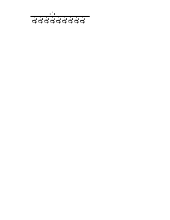
Figure 1: Physical model for Klein–Gordon equation. Cord and elastic elements

The solution can be obtained in a standard way. Introduce the Fourier transforms in the $t$ and $x$ domains:

$$\mathcal{F}_{t}[s](\omega)\equiv\frac{1}{2\pi}\int\limits_{-\infty}^{\infty}s(t)e^{i\omega t}dt,\qquad\mathcal{F}_{t}^{-1}[S](t)\equiv\int\limits_{-\infty}^{\infty}S(\omega)e^{-i\omega t}d\omega,$$ (2)

$$\mathcal{F}_{x}[s](k)\equiv\frac{1}{2\pi}\int\limits_{-\infty}^{\infty}s(t)e^{-ikx}dx,\qquad\mathcal{F}_{x}^{-1}[S](x)\equiv\int\limits_{-\infty}^{\infty}S(k)e^{ikx}dk.$$ (3)

For the Fourier image $U(\omega,k)$ of $u(t,x)$, get

$$(-c^{2}k^{2}+\omega^{2}-\omega_{\rm co}^{2})U(\omega,k)=\frac{1}{4\pi^{2}}.$$

The inverse Fourier transforms in $k$ and $t$ yields the double integral representation of the field:

$$u(t,x)=\frac{1}{4\pi^{2}}\int\limits_{-\infty+i\epsilon}^{\infty+i\epsilon}\int\limits_{-\infty}^{\infty}\frac{e^{ikx-i\omega t}}{\omega^{2}-c^{2}k^{2}-\omega_{\rm co}^{2}}dk\,d\omega.$$ (4)

The contours of integration are chosen according to the causality principle.

The denominator of (4) is referred to as the dispersion function. Its zeros defined by the dispersion equation

$$D(\omega,k)=\omega^{2}-c^{2}k^{2}-\omega_{\rm co}^{2}=0$$ (5)

correspond to modes in the waveguide.

The dispersion equation (5) has order $n=1$ with respect to $K=k^{2}$ and $W=\omega^{2}$. The solution of this equation is given by $\pm k(\omega)$, where

$$k(\omega)=c^{-1}\sqrt{\omega^{2}-\omega_{\rm co}^{2}}.$$ (6)

As the value of $\sqrt{\cdot}$, we select the branch of the square root that is close to $i\omega_{\rm co}$ when $\omega$ is close to zero. One can see that for all $\omega$ with ${\rm Im}[\omega]=\epsilon$ the imaginary part of $k(\omega)$ is positive.

The graphs of the dispersion diagram in the coordinates $(\omega,k)$ and $(W=\omega^{2},K=k^{2})$ are shown in Fig. 2.

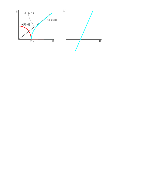
Figure 2: Dispersion diagram for a scalar Klein–Gordon equation

3 The field and its analysis

Start from the double–integral representation (4). Take $x>0$. Close the contour of integration with respect to $k$ in the upper half-plane. For each $\omega$ the integrand has two poles, $k=\pm k(\omega)$, and only the pole $k=k(\omega)$ belongs to the upper half-plane. Thus, by applying the residue theorem we obtain

$$u(t,x)=-\frac{i}{4\pi c}\int\limits_{-\infty+i\epsilon}^{\infty+i\epsilon}\frac{e^{ik(\omega)x-i\omega t}}{\sqrt{\omega^{2}-\omega_{\rm co}^{2}}}d\omega.$$ (7)

The integral can be easily taken:

$$u(t,x)=\left\{\begin{array}[]{ll}-(2c)^{-1}J_{0}(\omega_{\rm co}\sqrt{t^{2}-x^{2}/c^{2}}),&t>x/c,\\ 0,&0<t<x/c,\end{array}\right.$$ (8)

where $J_{0}$ is the Bessel function.

The following features of the solution should be mentioned:

• The front of the wave propagates with the speed equal to $c$. Near the front, the system behaves similarly to the usual wave equation. Only the cord shown in Fig. 1 plays role there, not the additional elastic elements. One can see that the shape of the front is the Heaviside function. The field before the front, i. e. for $t<x/c$, is equal to zero.

• For $t\gg x/c$ the system displays oscillations in time having the frequency tending to the cut-off $\omega_{\rm co}$. This means that far behind the front there exist oscillations with a small wavenumber and produced mainly by the elastic elements.

These features agree with the common understanding of the dispersion diagram (Fig. 2). The group velocity depends on $\omega$ as

$$v_{\rm gr}=\left(\frac{dk}{d\omega}\right)^{-1}=c\frac{\sqrt{\omega^{2}-\omega_{\rm co}^{2}}}{\omega},\qquad\omega_{\rm co}<\omega<\infty.$$ (9)

One can see that the group velocity grows from $0$ to $c$ as $\omega$ grows from $\omega_{\rm co}$ to $\infty$.

One can roughly imagine the wave process in the Klein–Gordon system as follows. First, the fast wave in the cord carries the energy over the waveguide. Next, the energy manifests itself in almost in-phase oscillations with frequency $\omega_{\rm co}$.

4 Complex parametrization of the dispersion diagram

Let us study the dispersion equation (5) for complex $\omega$ and $k$. The set of solutions of (5) is an analytic manifold $\mathfrak{H}$ of complex dimension 1 in the space $(\omega,k)\in\mathbb{C}^{2}$. Thus, $\mathfrak{H}$ has real dimension 2 in the space of real dimension 4. Let us build a parametrization of $\mathfrak{H}$ by a complex variable $\xi$ without using branching functions (i. e. square roots). This parametrization is as follows:

$$\omega=\omega_{\rm co}\sin\xi,\qquad k=i\frac{\omega_{\rm co}}{c}\cos\xi,$$ (10)

i. e. for each complex $\xi$ the point $(\omega,k)$ defined by (10) obeys (5), and for each solution of (5) there exists a corresponding $\xi$. One can see that the trigonometric functions in (10) are periodic with (real) period $2\pi$. Thus, it would be natural to consider $\xi$ being defined on a tube $\mathfrak{T}$, i. e. on a strip $-\pi/2\leq{\rm Re}[\xi]\leq 3\pi/2$ with the edges attached to each other (see Fig. 3, left).

Formulae (10) establish a bijection between $\mathfrak{T}$ and $\mathfrak{H}$. This means that the complex dispersion diagram $\mathfrak{H}$ is topologically a tube.

Manifold $\mathfrak{H}$ is embedded in $\mathbb{C}^{2}$ analytically since the derivatives $d\omega/d\xi$ and $dk/d\xi$ are not equal to zero simultaneously. Variable $\xi$ can be used as a local variable on $\mathfrak{H}$ everywhere (in the context of analytic manifolds).

The Riemann surface $\mathfrak{R}$ of the function $k(\omega)$ defined by (6) has two sheets cut along the segment $[-\omega_{\rm co},\omega_{\rm co}]$. The points $\pm\omega_{\rm co}$ are branch points of the surface, both having second order. The scheme of this Riemann surface is shown in Fig. 3, right. In the scheme, we mark by equal Roman numbers the shores of the cut attached to each other. Indeed, $\mathfrak{R}$ topologically is a tube as well.

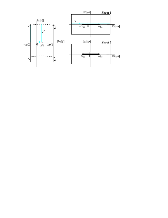
Figure 3: Tube $\mathfrak{T}$ of the variable $\xi$ (left). The Riemann surface $\mathfrak{R}$ (right)

Consider the representation (7). Let us rewrite it in the following form:

$$u(t,x)=-\frac{i}{4\pi c^{2}}\int_{\gamma}\frac{e^{ik(\omega)-i\omega t}}{k(\omega)}d\omega.$$ (11)

Contour $\gamma$ is $(-\infty+i\epsilon,\infty+i\epsilon)$ passed in the positive direction. Using the new variable $\xi$, the integral (11) can be rewritten using variable $\xi$:

$$u(t,x)=-\frac{1}{4\pi c}\int_{\gamma^{\prime}}e^{ik(\xi)x-i\omega(\xi)t}d\xi,$$ (12)

where $k(\xi)$ and $\omega(\xi)$ are defined by (10), and the contour $\gamma^{\prime}$ is shown in Fig. 3.

Thus, the integration is performed on $\mathfrak{T}$ or on $\mathfrak{H}$. We can say that the representation of the field can be interpreted as an integral over some contour drawn on the dispersion diagram $\mathfrak{H}$. This statement remains true when a general waveguide is considered. We remind that one can define contour integration on any analytic manifold of complex dimension 1 (see [5]), and the Cauchy’s theorem remains valid, i. e. one can deform the integration contour on the manifold. Indeed, the differential 1-form that is integrated over the contour should be holomorphic, which is generally the case.

5 Deformation of the integration contour

The contour of integration $\gamma^{\prime}$ can be deformed freely in the finite part of $\mathfrak{T}$. We also study admissible manipulations with the ‘‘tails’’ of $\gamma^{\prime}$ going to infinity, i. e. we study the possibilities of closing the contour.

The first sheet of $\mathfrak{R}$ corresponds to the domain ${\rm Im}[\xi]>0$ of $\mathfrak{T}$. Respectively, the second sheet corresponds to ${\rm Im}[\xi]<0$. The cut corresponds to the real segment $-\pi/2\leq\xi\leq 3\pi/2$ is cutting $\mathfrak{T}$ into two parts.

There are two outlets of the tube, namely ${\rm Im}[\xi]\to\infty$ and ${\rm Im}[\xi]\to-\infty$. These outlets are ‘‘infinities’’, in other words, $|\omega|\to\infty$ there.

Let be $t>x/c$. Consider the exponential factor (the integrand of (12)) on the tube $\mathfrak{T}$. The domains of exponential growth and decay of the exponential factor in this case are shown in Fig. 4, left. One can see that

$$\exp\{ik(\omega)-i\omega t\}=\exp\left\{i\omega_{\rm co}\left(\frac{ix}{c}\cos\xi-t\sin\xi\right)\right\}=\exp\{i\omega_{\rm co}r\cos(\xi-\eta)\},$$ (13)

where $r$ and $\eta$ are coordinates linked to $t$ and $x$ by

$$\frac{ix}{c}=r\cos\eta,\qquad-t=r\sin\eta.$$ (14)

The inverse coordinate change is

$$r=\sqrt{t^{2}-x^{2}/c^{2}},\qquad\eta={\rm atan}(ict/x).$$ (15)

Parameter $r$ is positive real, and parameter $\eta$ takes values on the half-line

$$\eta\in(-\pi/2,-\pi/2+i\infty).$$

As we mentioned above, the Cauchy’s theorem is valid on $\mathfrak{T}$, thus the integration contour can be deformed on $\mathfrak{T}$. Moreover, one can add some remote segments/arcs to the contour $\gamma^{\prime}$ in the domain of decay of the exponential factor, or, the same, to deform the tails of $\gamma^{\prime}$ in the domain of exponential decay.

Add an infinitely remote segment shown by the dashed line in Fig. 4, left. As the result, contour $\gamma^{\prime}$ becomes a closed loop going around the tube. It can be transformed into the real segment $[-\pi/2,3\pi/2]$.

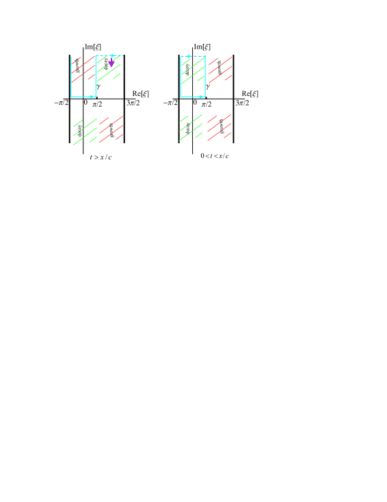
Figure 4: Domains of exponential growth and decay of the integrand of (7) for $t>x/c$ (left), and for $0<t<x/c$ (right)

If $0<t<x/c$, the consideration can be made again, and the domains of growth and decay become having form shown in Fig. 4, right. The way to close the contour is shown in the figure by a dashed line. One can see that the contour encircles a domain having no singularities, and thus the integral is equal to zero.

The consideration above has been made in terms of $\mathfrak{T}$ and the ‘‘natural’’ variable $\xi$. The same consideration can be translated into the language of the variable $\omega$ and the Riemann surface $\mathfrak{R}$. The closings of the integration contour $\gamma$ in the cases $t>x/c$ and $0<t<x/c$ are shown in Fig. 5. Indeed, the consideration in the variable $\omega$ is completely equivalent to the consideration in the variable $\xi$.

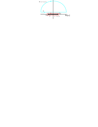
Figure 5: Closings of the integration contour on $\mathfrak{R}$ for $t>x/c$ (red) and for $0<t<x/c$ (blue)

We can make the following statements:

• The fact that the field before the front ($0<t<x/c$) is equal to zero has a topological nature. The field is equal to zero because $\gamma^{\prime}$ can be closed in such a way that it becomes homological to a zero contour.

• After the front ($t>x/c$) the contour encircles the ‘‘neck’’ of the tube. According to the Cauchy’s theorem, one can take any of such contours. Below we choose a contour that passes through the saddle points of the integrand of (12).

6 ‘‘Far–field’’ asymptotics of the solution

Let be $t>x/c$. Compute asymptotic estimations of the field directly from (11), i. e. without using the solution (8). First, perform the formal saddle-point analysis. Introduce the the parameter $V=x/t$ and assume that $x\to\infty$ while $V$ is fixed.

The integrand of (11) contains the exponential factor

$$\exp\{ik(\omega)x-i\omega t\}=\exp\{ix(k(\omega)-V^{-1}\omega)\}.$$

For building an asymptotic representation for $u(t,x)=u(x/V,x)$, one should find the stationary points of the function $k(\omega)-V^{-1}\omega$. We are looking for the saddle points $\omega_{*}$ such that

$$\frac{dk(\omega_{*})}{d\omega}=V^{-1}.$$ (16)

Note that this condition is equivalent to $v_{\rm gr}=V$.

According to (6), the saddle–points are $\pm\omega_{*}$,

$$\omega_{*}=\omega_{\rm co}\left(1-V^{2}/c^{2}\right)^{-1/2}.$$ (17)

In the variable $\xi$, the saddle–points corresponding to $\pm\omega_{*}$ are $\xi_{*}$ and $\xi_{*}-\pi$, where $\xi_{*}=\eta+\pi$.

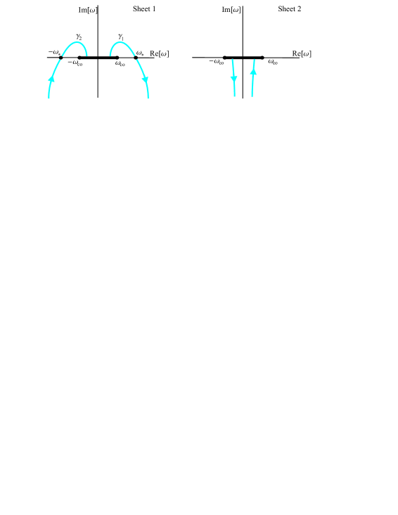
Figure 6: Steepest descend contours on $\mathfrak{R}$

Let us build the steepest descend contours passing through the saddle-points. As it is known, they are the contours on which the value ${\rm Re}[k(\omega)-V^{-1}\omega]$ is constant. The sketch of these contours is shown in Fig. 6. One can see that contour $\gamma$ can be transformed into the sum of the steepest descend contours $\gamma_{1}$ and $\gamma_{2}$ passing through $\omega_{*}$ and $-\omega_{*}$, respectively.

The integral can be estimated by the saddle–point expressions. The representations corresponding to the points $\omega_{*}$ and $-\omega_{*}$ are

$$u_{\pm\omega_{*}}(t,\omega)\approx-\frac{1}{2c}\frac{\exp\{\mp i\omega_{\rm co}\sqrt{t^{2}-x^{2}/c^{2}}\pm i\pi/4\}}{\sqrt{2\pi\omega_{\rm co}}\left(t^{2}-x^{2}/c^{2}\right)^{1/4}}.$$ (18)

The sum of these terms provide, indeed, a large-argument asymptotics for (8). This asymptotics is valid for a large argument of Bessel function, i. e. for

$$\omega_{\rm co}\sqrt{t^{2}-x^{2}/c^{2}}\gg 1.$$ (19)

7 ‘‘Near–field’’ asymptotics of the solution

Consider the integral (12). Our aim is to obtain the near-field asymptotics. Conversely to the concept of the far–field, where the exponential factor should be rapidly oscillating, here we are trying to find a contour integration (homotopic to $\gamma^{\prime}$) on which the exponential factor does not change considerably. In this case the integrand can be substituted by a constant.

Consider the contour $\gamma^{\prime}$ that is the segment $\gamma^{\prime}=[\eta,\eta+2\pi]$, or, the same $\gamma^{\prime}=[\xi_{*}-\pi,\xi_{*}+\pi]$. According to formula (13), the exponential term changes on this contour weakly if $r\omega_{\rm co}\ll 1$ or if

$$\omega_{\rm co}\sqrt{t^{2}-x^{2}/c^{2}}\ll 1.$$ (20)

The contour $\gamma^{\prime}$ in the $\xi$-domain is shown in Fig. 7, left. The image of this contour in the $\omega$-domain is shown in Fig. 7, right. The contour passes through the points $\eta=\xi_{*}-\pi$ and $\xi_{*}$. In the $\omega$-plane their images are the saddle–points $-\omega_{*}$, $\omega_{*}$ defined by (17). Note if the point $(t,x)$ is close to the wave front (i. e. if $t-x/c$ is small), the contour of integration in the $\omega$-domain is a large ellipse.

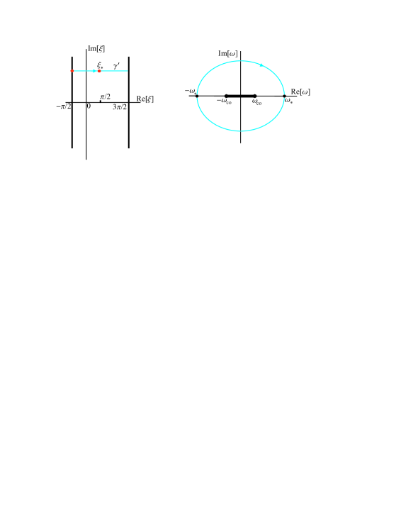
Figure 7: Integration contour for getting the near-field asymptotics (21)

Under this condition, a simple estimation of the integral (12) can be obtained. Since the exponential factor changes slightly, the exponential factor can be estimated by the constant $\exp\{i\omega_{\rm co}r\cos\eta\}$, and this constant is close to 1. Thus,(12) can be estimated as

$$u(t,x)\approx-\frac{1}{2c},$$ (21)

which is, indeed, an asymptotics of (8) for small values of the argument of Bessel function. The condition of validity (20) makes sense: the argument of Bessel function in (7) is close to zero in this case, and the value of Bessel function is close to 1.

8 Acknowledgements

The work is supported by the RFBR grant 19-29-06048.

References

- [1] A. Ben-Menahem and S. J. Singh. Seismic waves and sources. Springer Science & Business Media, 2012.
- [2] C. L. Pekeris. THEORY OF PROPAGATION OF EXPLOSIVE SOUND IN SHALLOW WATER. In Geological Society of America Memoirs, pages 1–116. Geological Society of America, 1948.
- [3] M. Muller, P. Moilanen, E. Bossy, P. Nicholson, V. Kilappa, J. Timonen, M. Talmant, S. Cheng, and P. Laugier. Comparison of three ultrasonic axial transmission methods for bone assessment. Ultrasound in Medicine & Biology, 31(5):633–642, may 2005.
- [4] B. Aalami. Waves in prismatic guides of arbitrary cross section. Journal of Applied Mechanics, 40(4):1067–1072, dec 1973.
- [5] B. V. Shabat. Introduction to Complex Analysis, Part 2; Functions of Several Variables. American Mathematical Society, 1992.